Credit Risk: Intro and Merton Model

Zhiguo He

University of Chicago

Booth School of Business

July, 2018, SAIF

OUTLINE

A GENTLE INTRODUCTION

THE MERTON MODEL

Pricing credit riskPredicting credit risk

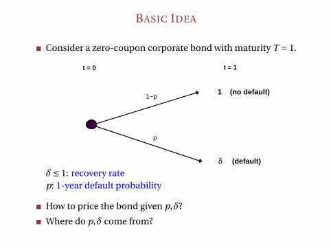
BASIC IDEA

Consider a zero-coupon corporate bond with maturity T = 1.

t = 0

1−p

p

t = 1

δ (default)

1 (no default)

δ≤ 1: recovery ratep: 1-year default probability

How to price the bond given p,δ?

Where do p,δ come from?

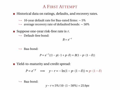
A FIRST ATTEMPT

Historical data on ratings, defaults, and recovery rates.

,→ 10-year default rate for Baa-rated firms: ∼ 5%,→ average recovery rate of defaulted bonds: ∼ 50%

Suppose one-year risk-free rate is r.,→ Default-free bond:

B = e−r

,→ Baa-bond:

P = e−r((1−p) ·1+p ·δ) = B(1−p · (1−δ))

Yield-to-maturity and credit spread:

P = e−y =⇒ y− r =− ln(1−p · (1−δ)) ≈ p · (1−δ)

,→ Baa-bond:y− r ≈ 5%/10 · (1−50%) = 25bps

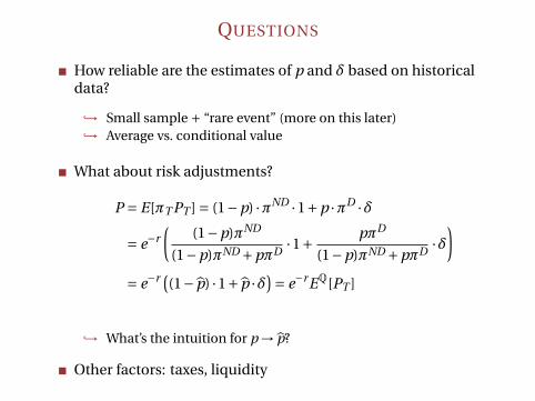
QUESTIONS

How reliable are the estimates of p and δ based on historicaldata?

,→ Small sample + “rare event” (more on this later),→ Average vs. conditional value

What about risk adjustments?

P = E[πT PT ] = (1−p) ·πND ·1+p ·πD ·δ

= e−r(

(1−p)πND

(1−p)πND +pπD·1+ pπD

(1−p)πND +pπD·δ

)= e−r (

(1− p̂) ·1+ p̂ ·δ)= e−rEQ[PT ]

,→ What’s the intuition for p → p̂?

Other factors: taxes, liquidity

OUTLINE

A GENTLE INTRODUCTION

THE MERTON MODEL

Pricing credit riskPredicting credit risk

THE MERTON MODEL

The fundamental challenge of limited data remains forreduced-form approach (especially for aggregate componentsof default risk, and for the Chinese market).

Structural models: impose structural assumptions to modeldefault (and capital structure) decisions.

A firm finances its operation by issuing both equity and debt. Itstotal asset value is Vt . Assume the firm issues a zero couponbond with face value F and maturity T .

Possible outcomes for debt holders at maturity T :1. VT > F =⇒ the firm sells some assets and pay the debt holders

2. VT < F =⇒ the firm is unable to pay debt holders in full

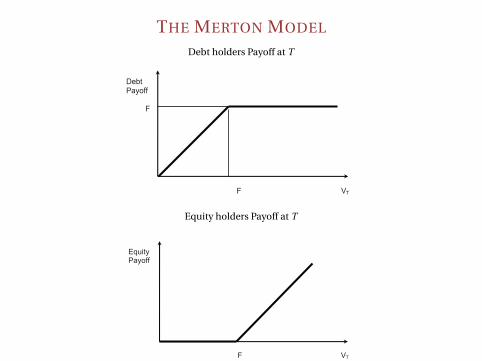
THE MERTON MODEL

Debt holders Payoff at T

DebtPayoff

F

F VT

Equity holders Payoff at T

EquityPayoff

F VT

A STRUCTURAL CREDIT RISK MODEL

Probability of default at T (between [0,T ]) = Pr(VT < F)

Need a model for Vt

Merton (1974): Assume the firm’s return on (market) assetsbetween 0 and T is log-normally distributed:

dVt =µVtdt +σVtdZt

This implies a log-normally distributed VT , from which we caneasily compute Pr(VT < F).

VT = V0 ×e(µ− 1

2σ2)T+σpTε

Using the B-S analogy, we can also price the bond (and equity)and derive the credit spread.

VALUE OF EQUITY – ANALOGY TO BLACK-SCHOLES

The payoff to equity holders is just like a call option on the stock:

max(VT −F ,0)

While B-S models stock price as lognormal, we have firm valueas lognormal.

We can simply apply Black and Scholes formula and obtain

E0 = Call (V0,F ,r,T ,σ)

where Call (V0,F ,r,T ,σ) is given by the Black-Scholes formula

VALUE OF EQUITY

Call (V0,F ,r,T ,σ) = V0 N(d1)−F e−rT N(d2)

d1 =ln

(V0F

)+ (

r+σ2/2)

T

σp

T; d2 = d1 −σ

pT

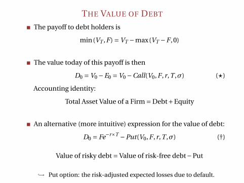
THE VALUE OF DEBT

The payoff to debt holders is

min(VT ,F) = VT −max(VT −F ,0)

The value today of this payoff is then

D0 = V0 −E0 = V0 −Call(V0,F ,r,T ,σ) (?)

Accounting identity:

Total Asset Value of a Firm = Debt+Equity

An alternative (more intuitive) expression for the value of debt:

D0 = Fe−r×T −Put(V0,F ,r,T ,σ) (†)

Value of risky debt = Value of risk-free debt−Put

,→ Put option: the risk-adjusted expected losses due to default.

CREDIT SPREADS

Credit Spread = YTM on corporate bond−YTM on Tresuary

From the definition of yield to maturity y for a corporate bond,we have:

D0 = e−y×T ×F =⇒ Fe−r×T −Put(V0,F ,r,T ,σ) = e−y×T F

which implies

e−r×T −Put

(V0

F,1,r,T ,σ

)= e−y×T

1−er×T ×Put

(V0

F,1,r,T ,σ

)= e−(y−r)×T

Credit Spread = y− r =− 1

Tlog

[1−er×T Put

(V0

F,1,r,T ,σ

)]

CREDIT SPREADS UNDER THE MERTON MODEL

0 1 2 3 4 5 6 7 8 9 10−0.05

0

0.05

0.1

0.15

0.2

0.25

0.3

time to maturity

cre

dit s

pre

ad

(%

)

Asset Volatility σ = 10%

D/A=.9D/A=.8D/A=.5

0 1 2 3 4 5 6 7 8 9 10−0.5

0

0.5

1

1.5

2

2.5

3

time to maturity

cre

dit s

pre

ad

(%

)

Asset Volatility σ = 20%

D/A=.9D/A=.8D/A=.5

Issues: (A) They are small; (B) They converge to zero at T → 0

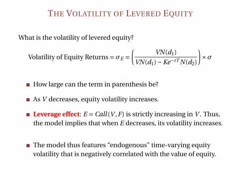
THE VOLATILITY OF LEVERED EQUITY

What is the volatility of levered equity?

Volatility of Equity Returns =σE =(

VN(d1)

VN(d1)−Ke−rT N(d2)

)×σ

How large can the term in parenthesis be?

As V decreases, equity volatility increases.

Leverage effect: E = Call (V ,F) is strictly increasing in V . Thus,the model implies that when E decreases, its volatility increases.

The model thus features “endogenous” time-varying equityvolatility that is negatively correlated with the value of equity.

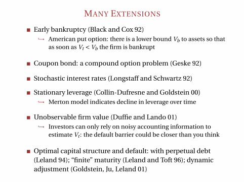
MANY EXTENSIONS

Early bankruptcy (Black and Cox 92),→ American put option: there is a lower bound Vb to assets so that

as soon as Vt < Vb the firm is bankrupt

Coupon bond: a compound option problem (Geske 92)

Stochastic interest rates (Longstaff and Schwartz 92)

Stationary leverage (Collin-Dufresne and Goldstein 00),→ Merton model indicates decline in leverage over time

Unobservable firm value (Duffie and Lando 01),→ Investors can only rely on noisy accounting information to

estimate Vt : the default barrier could be closer than you think

Optimal capital structure and default: with perpetual debt(Leland 94); “finite” maturity (Leland and Toft 96); dynamicadjustment (Goldstein, Ju, Leland 01)

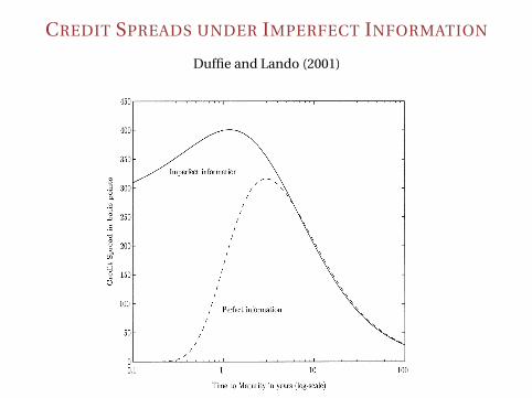
CREDIT SPREADS UNDER IMPERFECT INFORMATION

Duffie and Lando (2001)

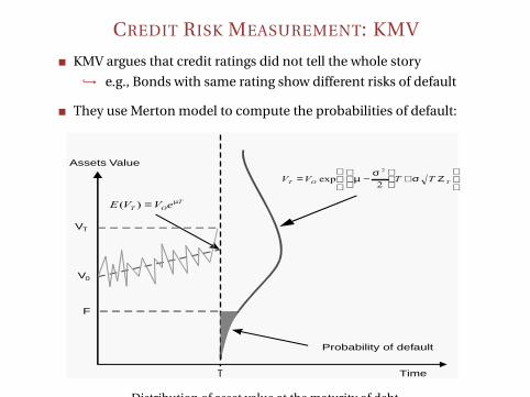
CREDIT RISK MEASUREMENT: KMV

KMV argues that credit ratings did not tell the whole story

,→ e.g., Bonds with same rating show different risks of default

They use Merton model to compute the probabilities of default:

Assets Value

VT

V0

Probability of default

Time

F

= µ

= −

+

µσ

σ Ζ

Fig. 7. Distribution of the ®rmÕs assets value at maturity of the debt obligation.

Distribution of asset value at the maturity of debt.

CREDIT RISK MEASUREMENT: KMV

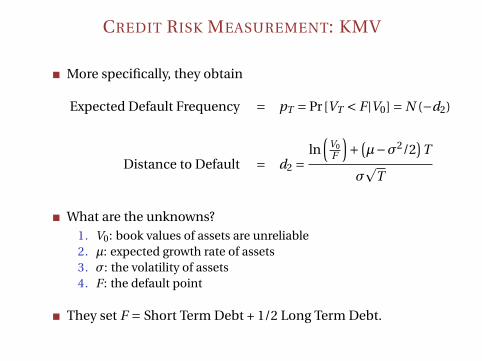
More specifically, they obtain

Expected Default Frequency = pT = Pr[VT < F |V0] = N (−d2)

Distance to Default = d2 =ln

(V0F

)+ (

µ−σ2/2)

T

σp

T

What are the unknowns?1. V0: book values of assets are unreliable2. µ: expected growth rate of assets3. σ: the volatility of assets4. F : the default point

They set F = Short Term Debt + 1/2 Long Term Debt.

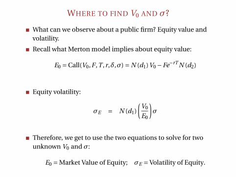
WHERE TO FIND V0 AND σ?

What can we observe about a public firm? Equity value andvolatility.

Recall what Merton model implies about equity value:

E0 = Call(V0,F ,T ,r,δ,σ) = N (d1)V0 −Fe−rT N (d2)

Equity volatility:

σE = N (d1)

(V0

E0

)σ

Therefore, we get to use the two equations to solve for twounknown V0 and σ:

E0 = Market Value of Equity; σE = Volatility of Equity.

CREDIT RISK MEASUREMENT: KMV

Simple Example (KMV model is much more elaborate):,→ Enron market capitalization on May 30 1989 was 2.260 bil,→ The book value of debt = 3.249 bil (prospectus),→ Volatility of equity return = 20%,→ The nominal one year interest rate was 8.6% (continuously

compounded),→ Assume T = 8 years (long term debt)

Next two figures plot the value of equity and volatility of equityimplied by the Merton model for various levels of current assetsV0 and volatility σ

Enron Corp Returns and Volatility

1986 1986.5 1987 1987.5 1988 1988.5 1989 1989.5−0.4

−0.3

−0.2

−0.1

0

0.1

0.2

0.3Enron Returns

1986 1986.5 1987 1987.5 1988 1988.5 1989 1989.50

20

40

60

80

100

120

140Enron Annualized Volatility

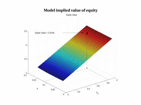
Model implied value of equity

33.2

3.43.6

3.84

0

0.05

0.1

0.15

0.21

1.5

2

2.5

V0

Equity Value

σ

Equity Value = 2.26 bil

Model implied volatility of equity

33.2

3.43.6

3.84

0

0.05

0.1

0.15

0.20

0.05

0.1

0.15

0.2

0.25

0.3

0.35

V0

Equity Volatility

σ

Equity Volatility = 20 %

We therefore find V0 = 3.84 bil and σ= 12%

We need one final input: the growth rate of assets µ. This must beforecasted from fundamentals.

Assume µ= 15%. We find:

d2 = 2.69 and pT = 0.36%

CREDIT RISK MEASUREMENT: KMV

KMV: normal distribution imperfect, especially the thin tails.

They estimate a new (non-parametric) mapping betweendistance to default and expected default frequency from data.

Distance to Default and Expected Default Frequency

Fig. 17. Mapping of the ``distance-to-default'' into the ``expected default frequencies'', for a given

time horizon.

Barath and Shumway (08): little evidence that KMV EDFoutperforms Merton model.

WHAT’S NEXT?

How to apply Merton model to banks?,→ Merton model assumes constant volatility for asset value. Bad

assumption for banks.,→ How to model asset volatility better? Big part of banks’ assets are

defaultable debt.,→ Use this feature to endogenously generate asset volatility. (Nagel

and Purnanandam 15),→ What about short term debt?

How to model SOE debt?

How to model government debt?