
Rating based credit risk models Jacek Jakubowski
118
Rating based credit risk models Jacek Jakubowski University of Warsaw B¸ edlewo, 2008, EMS school: Risk Theory and Related Topics 1
Transcript of Rating based credit risk models Jacek Jakubowski

Rating based credit risk models
Jacek Jakubowski
University of Warsaw
Bedlewo, 2008, EMS school: Risk Theory and Related Topics
1

Outline
I. Rating based term structure models
1. Bond market
2. HJM model and generalization of HJM - model driven by Lévy motion
3. The defaultable Lévy term structure model
a) Types of recovery
b) HJM condition
c) Model with rating migration
2

II. Modeling of credit migration processes
III. Pricing of rating based defaultable claims
3

• Bond market
T > 0 fixed horizon date for all market activities, probability space with filtration.
Let B(t, θ), 0 ≤ t ≤ θ be the market price of a zero-coupon bond at moment t.
B(t, θ) is strictly positive, B(θ, θ) = 1
4

• Bond market
T > 0 fixed horizon date for all market activities, probability space with filtration.
Let B(t, θ), 0 ≤ t ≤ θ be the market price of a zero-coupon bond at moment t.
B(t, θ) is strictly positive, B(θ, θ) = 1
Aim: to construct the family of prices in a consistent way.
4

• Bond market
T > 0 fixed horizon date for all market activities, probability space with filtration.
Let B(t, θ), 0 ≤ t ≤ θ be the market price of a zero-coupon bond at moment t.
B(t, θ) is strictly positive, B(θ, θ) = 1
Aim: to construct the family of prices in a consistent way.
• risk-free saving account with short term interest rate rt. If at moment 0 one puts into thebank account 1 unit of money then at moment t one has :
Bt = exp(
∫ t
0rudu)
What are connection between saving account process and bond price processes?
If short term interest rate is deterministic, then
B(t, θ) = e−∫ θ
trsds.
4

Definition 1. A family B(t, θ), 0 ≤ t ≤ θ ≤ T of adapted processes iscalled an arbitrage-free family of bond prices relatively to r if
i) B(θ, θ) = 1 for every θ ≤ T ,
ii) there exist a probability measure P ∗ such that B∗(t, θ) = B(t, θ)/Bt isa P ∗-martingale for any θ ≤ T .
Hence
B(t, θ) = EP ∗(e−∫ θt rsds|F t)
Conversely, given r, P ∗, the family B(t, θ) defined above is an arbitrage-free family of bond prices relatively to r.
5

• Model short term interest rate by Ito process
dr(t) = b(t)dt+ σ(t)dW (t).• Standard models:
Vasicek :
dr(t) = (b+ βr(t))dt+ σ(t)dW (t).
Cox, Ingersoll and Ross
dr(t) = (a− br(t))dt+ σ√r(t)dW (t),
where a, b, σ are constants with a ≥ 0, b > 0, σ > 0
• Most of models provide an affine term structure
B(t, θ) = exp(−A(t, θ)−B(t, θ)rt).
• Initial term structure:
B(0, θ) = EP ∗(e−∫ θ
0rsds), 0 ≤ θ ≤ T
Bond price models based on a specific short term interest rate process makes the problem
of matching the initial term structure.
6
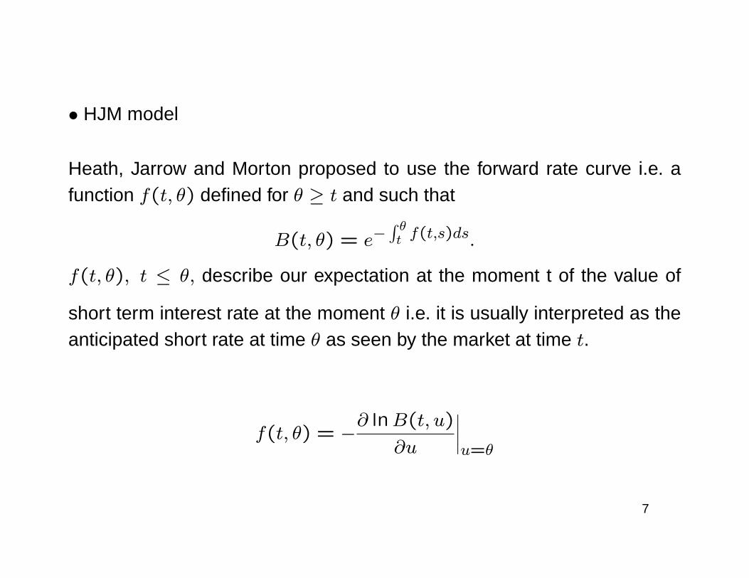
• HJM model
Heath, Jarrow and Morton proposed to use the forward rate curve i.e. afunction f(t, θ) defined for θ ≥ t and such that
B(t, θ) = e−∫ θt f(t,s)ds.
f(t, θ), t ≤ θ, describe our expectation at the moment t of the value of
short term interest rate at the moment θ i.e. it is usually interpreted as theanticipated short rate at time θ as seen by the market at time t.
f(t, θ) = −∂ lnB(t, u)
∂u
∣∣∣∣u=θ
7

Heath, Jarrow and Morton proposed to model the forward curves as Itôprocesses
df(t, θ) = α(t, θ)dt+ < σ(t, θ), dZ(t) >, 0 ≤ t ≤ θ, (1)
with Z d-dimensional standard Wiener process, defined on a filtered pro-bability space (Ω,F , (Ft),P ).
Equivalently, for t ≤ θ,
f(t, θ) = f(0, θ) +∫ t0α(s, θ) ds+
∫ t0< σ(s, θ), dZ(s) > . (2)
For each θ the processes α(t, θ), σ(t, θ), t ≤ θ, are assumed to be pre-dictable with respect to a given filtration (Ft) and such that integrals in (2)are well defined.
8

It is convenient to assume that once a bond has matured its cash equivalent goes to thebank account. Thus B(t, θ), the market price at time t of a bond paying 1 at the maturitytime θ, is defined also for t ≥ θ by the formula
B(t, θ) = e
∫ t
θr(σ) dσ
. (3)
For θ < t we put
α(t, θ) = σ(t, θ) = 0, (4)
so the forward rate f is defined for t, θ ∈ [0, T ]. By (4) we deduce from (2) that for t > θ,
f(t, θ) = f(0, θ) +
∫ θ
0α(s, θ) ds+
∫ θ
0< σ(s, θ), dZ(s) > .
Consequently, for each θ > 0 the process f(t, θ), t > θ, is constant in t and could beidentified with the short rate:
r(θ) = f(0, θ) +
∫ θ
0α(s, θ) ds+
∫ θ
0< σ(s, θ), dZ(s) > . (5)
So r(θ) = f(θ, θ) .
9

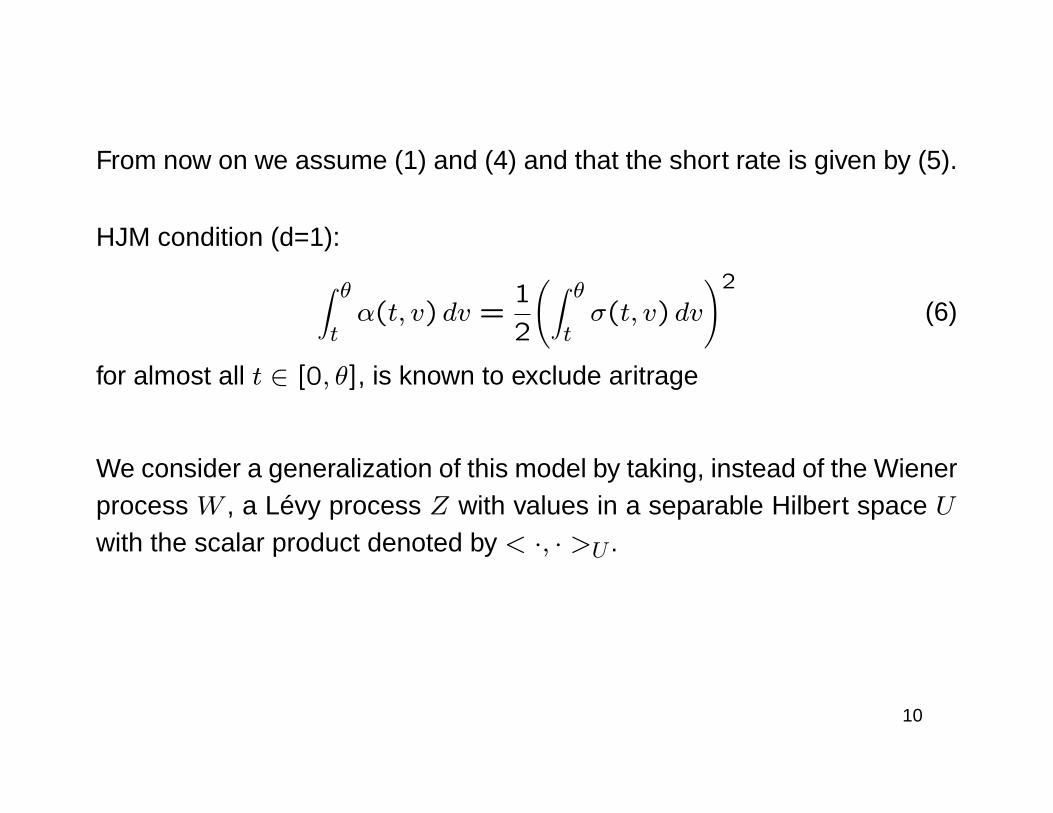
From now on we assume (1) and (4) and that the short rate is given by (5).
HJM condition (d=1):
∫ θtα(t, v) dv =
1
2
(∫ θtσ(t, v) dv
)2
(6)
for almost all t ∈ [0, θ], is known to exclude aritrage
10
From now on we assume (1) and (4) and that the short rate is given by (5).
HJM condition (d=1):
∫ θtα(t, v) dv =
1
2
(∫ θtσ(t, v) dv
)2
(6)
for almost all t ∈ [0, θ], is known to exclude aritrage
We consider a generalization of this model by taking, instead of the Wienerprocess W , a Lévy process Z with values in a separable Hilbert space Uwith the scalar product denoted by < ·, · >U .
10

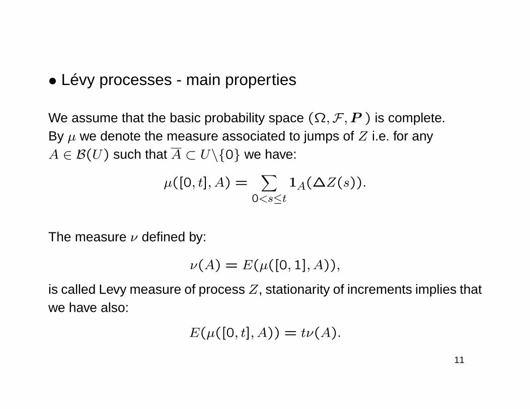
• Lévy processes - main properties
We assume that the basic probability space (Ω,F ,P ) is complete.By µ we denote the measure associated to jumps of Z i.e. for anyA ∈ B(U) such that A ⊂ U\0 we have:
µ([0, t], A) =∑
0<s≤t1A(∆Z(s)).
11
• Lévy processes - main properties
We assume that the basic probability space (Ω,F ,P ) is complete.By µ we denote the measure associated to jumps of Z i.e. for anyA ∈ B(U) such that A ⊂ U\0 we have:
µ([0, t], A) =∑
0<s≤t1A(∆Z(s)).
The measure ν defined by:
ν(A) = E(µ([0,1], A)),
is called Levy measure of process Z, stationarity of increments implies thatwe have also:
E(µ([0, t], A)) = tν(A).
11

The Lévy-Khintchine formula shows that characteristic function of Lévyprocess has a form:
Eei<λ,Z(t)>U = etψ(λ),
where
ψ(λ) =i < a, λ >U −1
2< Qλ, λ >U +∫
U(ei〈λ,x〉U − 1− i < x, λ >U 1[−1,1](|x|U))ν(dx),
and a ∈ U , Q is symmetric non negative nuclear operator on U , ν is ameasure on U with ν(0) = 0 and∫
U(|x|2 ∧ 1)ν(dx) <∞. (7)
12

Example. Let X be a compound Poisson, i.e.
Xt =Nt∑k=1
Yk,
where Yi are i.i.d., F = FY . Then
E(eiuXt) = exp(λt∫R(eiuy − 1)F (dy)
).
If E(eαY1) <∞, then
E(eαXt) = exp(λt∫R(eαy − 1)F (dy)
).
13

Moreover Z has a well known Lévy-Itô decomposition:
Z(t) =at+W (t) +∫ t0
∫|y|U≤1
y(µ(ds, dy)− dtν(dy))+∫ t0
∫|y|U>1
yµ(ds, dy),
where W is a Wiener process with values in U and covariance operator Q.
14
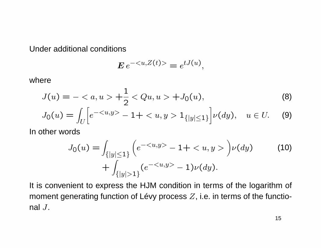
Under additional conditions
E e−<u,Z(t)> = etJ(u),
where
J(u) = − < a, u > +1
2< Qu, u > +J0(u), (8)
J0(u) =∫U
[e−<u,y> − 1+ < u, y > 1|y|≤1
]ν(dy), u ∈ U. (9)
In other words
J0(u) =∫|y|≤1
(e−<u,y> − 1+ < u, y >
)ν(dy) (10)
+∫|y|>1
(e−<u,y> − 1)ν(dy).
It is convenient to express the HJM condition in terms of the logarithm ofmoment generating function of Lévy process Z, i.e. in terms of the functio-nal J .
15

We will regard coefficients α and σ, in the equation (1) i.e. in :
df(t, θ) = α(t, θ)dt+ < σ(t, θ), dZ(t) >, 0 ≤ t ≤ θ,
as, respectively, H = L2([0, T ]), L(U,H) valued, predictable proces-ses:
α(t)(θ) = α(t, θ), θ ∈ [0, T ],
σ(t)u(θ) =< σ(t, θ), u > , u ∈ U, θ ∈ [0, T ].
Then (1) can be written as
df(t) = α(t)dt+ σ(t)dZ(t). (11)
16

Let us recall that HJM postulate is the requirement that the discountedbond price processes B∗(·, θ), θ ∈ [0, T ]:
B∗(t, θ) =B(t, θ)
Bt= e−
∫ θt f(t,s)dse−
∫ t0 f(t,s)ds = e−
∫ θ0 f(t,s)ds
are local martingales.
17

Let us recall that HJM postulate is the requirement that the discountedbond price processes B∗(·, θ), θ ∈ [0, T ]:
B∗(t, θ) =B(t, θ)
Bt= e−
∫ θt f(t,s)dse−
∫ t0 f(t,s)ds = e−
∫ θ0 f(t,s)ds
are local martingales.
Let b be the Laplace transform of the measure ν restricted to the comple-ment of the ball y : |y| ≤ 1,
b(u) =∫|y|>1
e−<u,y>ν(dy), (12)
and B the set of those u ∈ U for which the Laplace transform is finite:
B = u ∈ U : b(u) <∞.
17

Assumption:
(H1) Processes α and σ are predictable and, with probability one, havebounded trajectories.
(H2) For arbitary r > 0 the function b is bounded on
u : |u| ≤ r, b(u) <∞.
18

Theorem 1. Assume that (H1) holds.
i) If HJM postulate holds then, for arbitrary θ ≤ T , P − almost surely,∫ θtσ(t, v) dv ∈ B, (13)
for almost all t ∈ [0, θ].
ii) Assume (H2) and that for all θ ≤ T, P − almost surely (13) holdsfor almost all t ∈ [0, θ]. Then HJM postulate holds if and only if, thefollowing HJM condition is satisfied,∫ θ
tα(t, v) dv = J
(∫ θtσ(t, v) dv
), (14)
for almost all t ∈ [0, θ]
19
Remark 1. Explicit formulation (14), in terms of the function J , indicatesthat the drift term is completely determined by the diffusion term. In theparticular case when a = 0, µ = 0, one arrives at the classical HJMcondition.
20
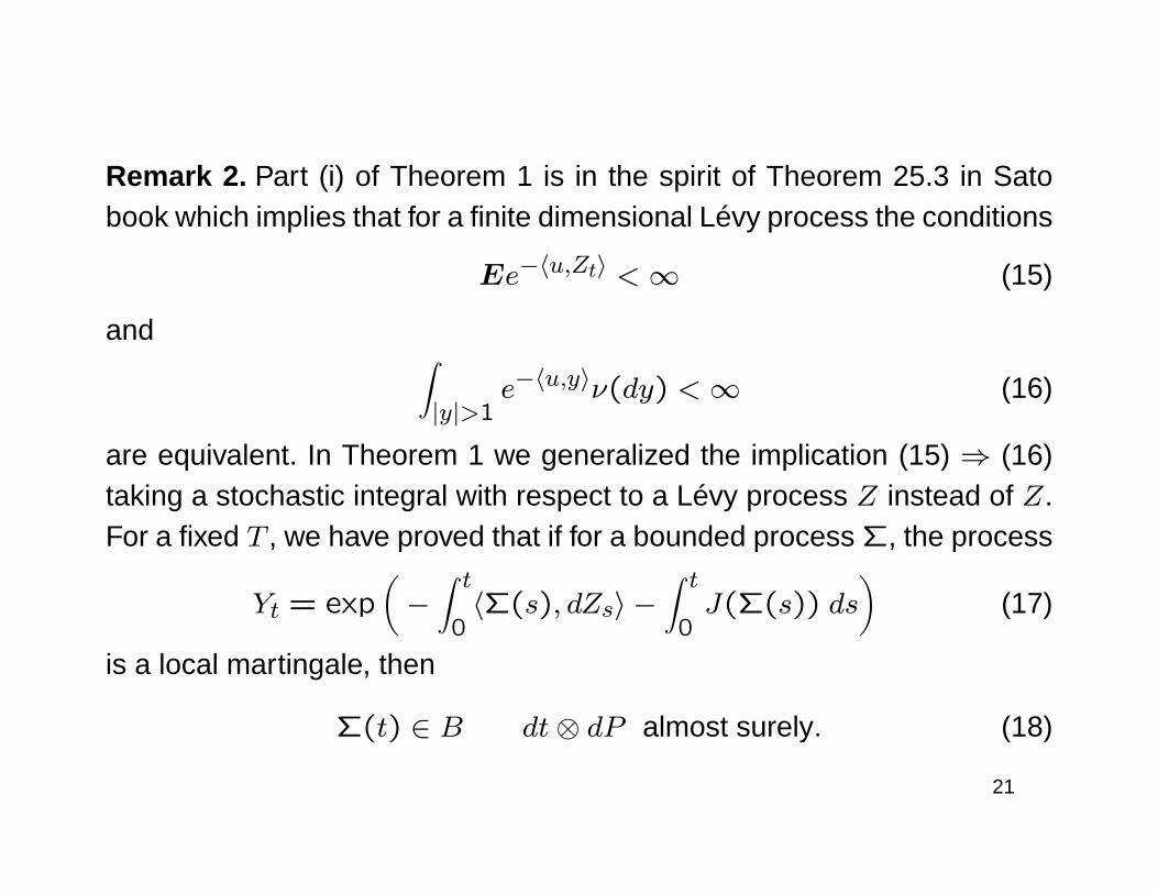
Remark 2. Part (i) of Theorem 1 is in the spirit of Theorem 25.3 in Satobook which implies that for a finite dimensional Lévy process the conditions
Ee−〈u,Zt〉 <∞ (15)
and ∫|y|>1
e−〈u,y〉ν(dy) <∞ (16)
are equivalent. In Theorem 1 we generalized the implication (15) ⇒ (16)taking a stochastic integral with respect to a Lévy process Z instead of Z.For a fixed T , we have proved that if for a bounded process Σ, the process
Yt = exp(−∫ t0〈Σ(s), dZs〉 −
∫ t0J(Σ(s)) ds
)(17)
is a local martingale, then
Σ(t) ∈ B dt⊗ dP almost surely. (18)
21

Remark 3. This condition, even in the finite dimensional case, is more ge-neral than that given in the paper by Eberlein and Özkan who assume thereexists a constant M > 0 such that∫
|y|>1e−〈c,y〉ν(dy) <∞ for all c ∈ [−M,M ]d. (19)
and the volatility function takes values in that interval. However, as followsfrom Theorem 1, if σ is a positive process and Z has only positive jumps,no a priori requirements on ν are necessary. Indeed, if a 1-dimensionalLévy process Z has positive jumps and the volatility is non-negative, thencondition (13) is always satisfied (condition (19) might not be satisfied).
22
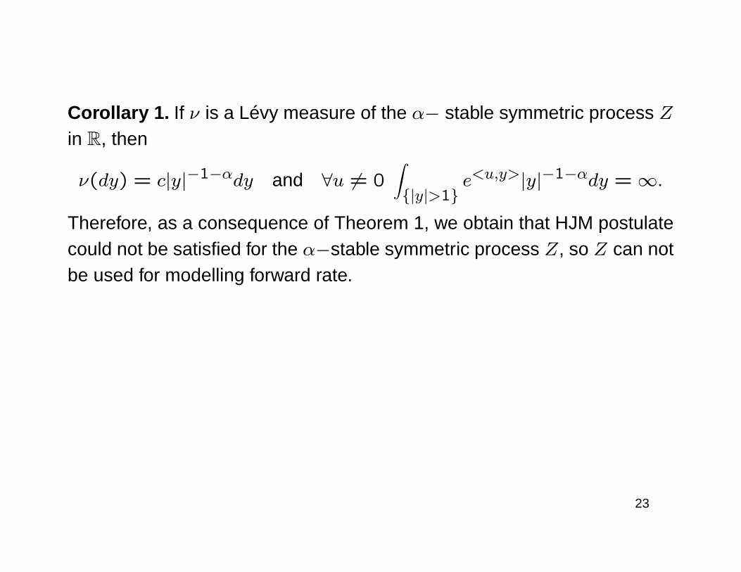
Corollary 1. If ν is a Lévy measure of the α− stable symmetric process Zin R, then
ν(dy) = c|y|−1−αdy and ∀u 6= 0∫|y|>1
e<u,y>|y|−1−αdy = ∞.
Therefore, as a consequence of Theorem 1, we obtain that HJM postulatecould not be satisfied for the α−stable symmetric process Z, so Z can notbe used for modelling forward rate.
23

Corollary 2. Under mild assumption the HJM-type condition can be writtenas
α(t, θ) =⟨DJ
( ∫ θ0σ(t, v)dv
), σ(t, θ)
⟩U,
where
DJ(x) = −a+Qx−∫U
(e−〈x,y〉U − 1|y|U≤1(y)
)y ν(dy),
so the HJM-type condition has the following form:
α(t, θ) = −⟨a, σ(t, θ)
⟩U
+⟨Q∫ θ0σ(t, v)dv, σ(t, θ)
⟩U
−∫U
(e−〈
∫ θ0 σ(t,v)dv,y〉U − 1|y|U≤1(y)
)⟨y, σ(t, θ)
⟩Uν(dy).
24

The dynamics of the forward rate f under the HJM condition.Theorem 2. Assume that∫
|y|≥1e−〈u,y〉ν(dy) <∞ (20)
for all u from some neighborhood of the set in which∫ θt σ(t, v)dv takes
values. Then the HJM condition (14) implies that the dynamics of f hasthe form
df(t, θ) =⟨DJ
( ∫ θtσ(t, v)dv
), σ(t, θ)
⟩dt+ 〈σ(t, θ), dZ(t)〉, (21)
where DJ is the gradient of J .
Thus, under very mild assumptions, the HJM postulate holds if and only if
df(t, θ) =⟨DJ
( ∫ θtσ(t, v) dv
), σ(t, θ)
⟩dt+ 〈σ(t, θ), dZ(t)〉.
25

Now I indicate the difference between finite and infinite dimensional case.
For U = Rd under a natural condition on the volatility σ the function b isfinite on a certain set.
Remark 4. Let U = Rd. If b is finite on a dense subset ofK and IntK 6= ∅,then
b(u) <∞ (22)
for all u ∈ IntK i.e. IntK ⊂ B.
26

Proof. We first prove that if U = Rd and (22) is satisfied on a dense subsetD of the open ball B(x, r), x ∈ Rd, r > 0, then it holds for all c ∈ B(x, r).Indeed, for every c ∈ B(x, r) there exist c1, . . . , cd+1 ∈ D such that
c belongs to the simplex with vertices c1, . . . , cd+1, i.e. c =∑d+1i=1 λici,
λi ∈ [0,1],∑d+1i=1 λi = 1. Hence, by convexity of the exponential function,
∫|y|>1
e−〈c,y〉ν(dy) ≤d+1∑i=1
λi
∫|y|>1
e−〈ci,y〉ν(dy) <∞,
since c1, . . . , cd+1 ∈ D.Next, sinceG = IntK is open, for every x ∈ G there exists r > 0 such thatB(x, r) ⊂ G. By assumption (22) holds for a dense subset of B(x, r), soby the previous considerations (22) holds for all y ∈ B(x, r), in particularfor y = x.
27

It turns out that many properties of B which hold in finite dimensions arenot true in infinite dimensions. In particular, in infinite dimensions the set Bcould be the difference of an open set and a dense subset.
Theorem 3. There exists a model of the form (1) for which (H1) holds, HJMpostulate is satisfied, ∫
|y|>1e−<c,y>ν(dy) <∞, (23)
for c in a dense subset of B(0, r),∫|y|>1
e−<cn,y>ν(dy) = ∞ (24)
for a sequence cn → 0 as n→∞.
28
HJM conditions for defaultable bonds
• Our aim is to derive the HJM-type conditions for the market
containing a risk free bond and defaultable bonds.
In a defaultable case we have several variants describing amount and ti-ming of so called recovery payment which is paid to bond holders if defaulthas occurred before bond’s maturity. If by τ we denote the moment of de-fault, then, generally speaking, the payoff of the defaultable bond is asfollows:
D(θ, θ) = 1τ>θ + 1τ≤θ · recovery payment .
29
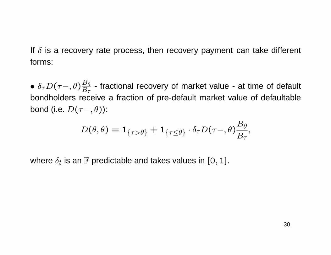
If δ is a recovery rate process, then recovery payment can take differentforms:
• δτD(τ−, θ)BθBτ - fractional recovery of market value - at time of defaultbondholders receive a fraction of pre-default market value of defaultablebond (i.e. D(τ−, θ)):
D(θ, θ) = 1τ>θ + 1τ≤θ · δτD(τ−, θ)BθBτ,
where δt is an F predictable and takes values in [0,1].
30
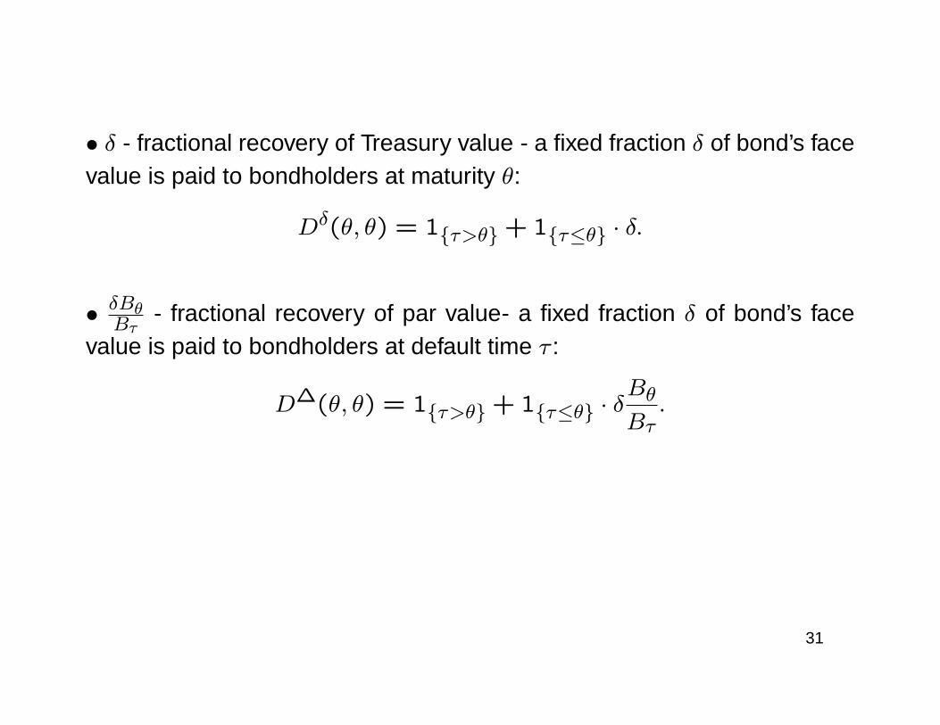
• δ - fractional recovery of Treasury value - a fixed fraction δ of bond’s facevalue is paid to bondholders at maturity θ:
Dδ(θ, θ) = 1τ>θ + 1τ≤θ · δ.
• δBθBτ
- fractional recovery of par value- a fixed fraction δ of bond’s facevalue is paid to bondholders at default time τ :
D∆(θ, θ) = 1τ>θ + 1τ≤θ · δBθBτ.
31
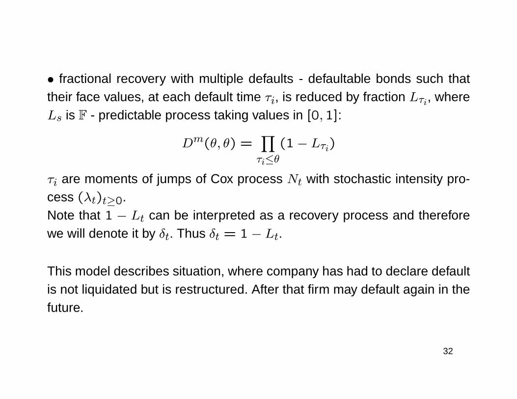
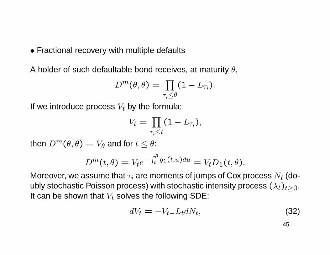
• fractional recovery with multiple defaults - defaultable bonds such thattheir face values, at each default time τi, is reduced by fraction Lτi, whereLs is F - predictable process taking values in [0,1]:
Dm(θ, θ) =∏τi≤θ
(1− Lτi)
τi are moments of jumps of Cox process Nt with stochastic intensity pro-cess (λt)t≥0.Note that 1 − Lt can be interpreted as a recovery process and thereforewe will denote it by δt. Thus δt = 1− Lt.
This model describes situation, where company has had to declare defaultis not liquidated but is restructured. After that firm may default again in thefuture.
32
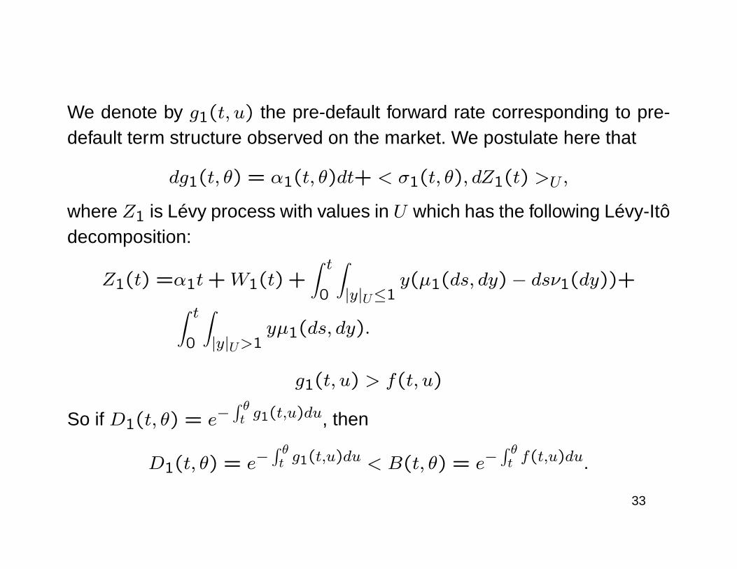
We denote by g1(t, u) the pre-default forward rate corresponding to pre-default term structure observed on the market. We postulate here that
dg1(t, θ) = α1(t, θ)dt+ < σ1(t, θ), dZ1(t) >U ,
where Z1 is Lévy process with values in U which has the following Lévy-Itôdecomposition:
Z1(t) =α1t+W1(t) +∫ t0
∫|y|U≤1
y(µ1(ds, dy)− dsν1(dy))+∫ t0
∫|y|U>1
yµ1(ds, dy).
g1(t, u) > f(t, u)
So if D1(t, θ) = e−∫ θt g1(t,u)du, then
D1(t, θ) = e−∫ θt g1(t,u)du < B(t, θ) = e−
∫ θt f(t,u)du.
33
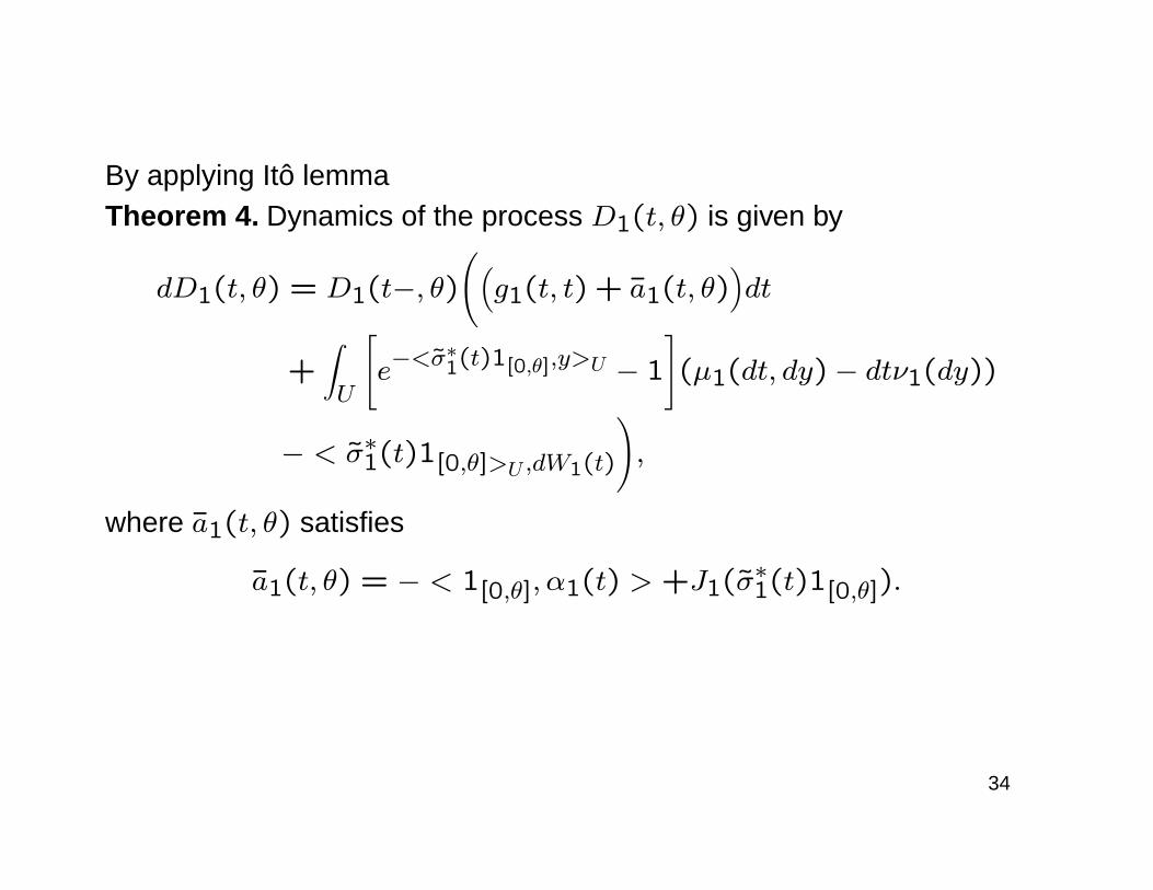
By applying Itô lemmaTheorem 4. Dynamics of the process D1(t, θ) is given by
dD1(t, θ) = D1(t−, θ)((g1(t, t) + a1(t, θ)
)dt
+∫U
[e−<σ
∗1(t)1[0,θ],y>U − 1
](µ1(dt, dy)− dtν1(dy))
− < σ∗1(t)1[0,θ]>U ,dW1(t)
),
where a1(t, θ) satisfies
a1(t, θ) = − < 1[0,θ], α1(t) > +J1(σ∗1(t)1[0,θ]).
34
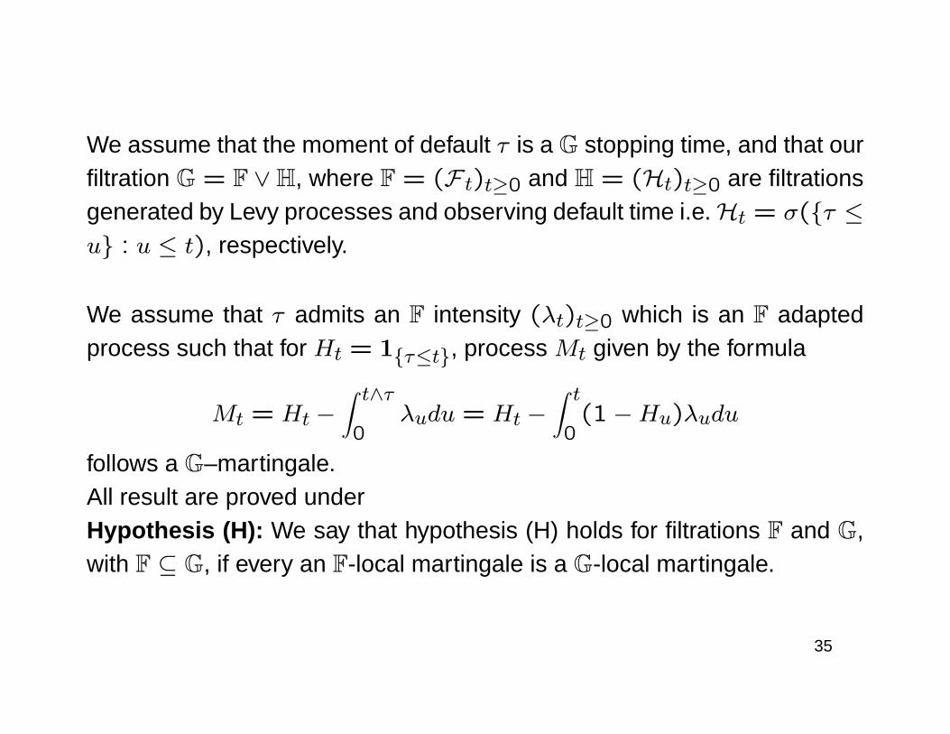
We assume that the moment of default τ is a G stopping time, and that ourfiltration G = F ∨H, where F = (F t)t≥0 and H = (Ht)t≥0 are filtrationsgenerated by Levy processes and observing default time i.e.Ht = σ(τ ≤u : u ≤ t), respectively.
We assume that τ admits an F intensity (λt)t≥0 which is an F adaptedprocess such that for Ht = 1τ≤t, process Mt given by the formula
Mt = Ht −∫ t∧τ0
λudu = Ht −∫ t0(1−Hu)λudu
follows a G–martingale.All result are proved underHypothesis (H): We say that hypothesis (H) holds for filtrations F and G,with F ⊆ G, if every an F-local martingale is a G-local martingale.
35
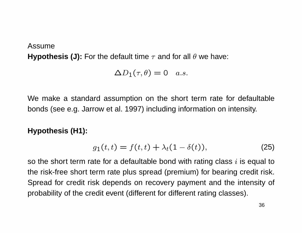
AssumeHypothesis (J): For the default time τ and for all θ we have:
∆D1(τ, θ) = 0 a.s.
We make a standard assumption on the short term rate for defaultablebonds (see e.g. Jarrow et al. 1997) including information on intensity.
Hypothesis (H1):
g1(t, t) = f(t, t) + λt(1− δ(t)), (25)
so the short term rate for a defaultable bond with rating class i is equal tothe risk-free short term rate plus spread (premium) for bearing credit risk.Spread for credit risk depends on recovery payment and the intensity ofprobability of the credit event (different for different rating classes).
36

Hypothesis (H1) is natural, which one can see from the following fact.
Remark 5. If the price of a defaultable bond with fractional recovery ofmarket value is given in traditional way, it means that it is given by theintensity proces λ and the risk-free short term rate r in the following way:
1τ>tD(t, θ) = 1τ>tE(e−∫ θt [ru+(1−δu)λu]du|F t);
then, for bounded λ and r, we have
37
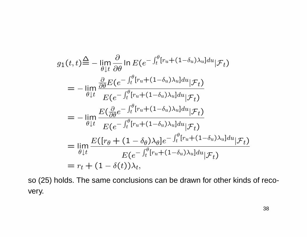
g1(t, t)∆=− lim
θ↓t∂
∂θlnE(e−
∫ θt [ru+(1−δu)λu]du|F t)
= − limθ↓t
∂∂θE(e−
∫ θt [ru+(1−δu)λu]du|F t)
E(e−∫ θt [ru+(1−δu)λu]du|F t)
= − limθ↓t
E( ∂∂θe−∫ θt [ru+(1−δu)λu]du|F t)
E(e−∫ θt [ru+(1−δu)λu]du|F t)
= limθ↓t
E([rθ + (1− δθ)λθ]e−∫ θt [ru+(1−δu)λu]du|F t)
E(e−∫ θt [ru+(1−δu)λu]du|F t)
= rt + (1− δ(t))λt,
so (25) holds. The same conclusions can be drawn for other kinds of reco-very.
38
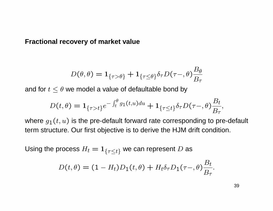
Fractional recovery of market value
D(θ, θ) = 1τ>θ + 1τ≤θδτD(τ−, θ)BθBτ
and for t ≤ θ we model a value of defaultable bond by
D(t, θ) = 1τ>te−∫ θt g1(t,u)du + 1τ≤tδτD(τ−, θ)
Bt
Bτ,
where g1(t, u) is the pre-default forward rate corresponding to pre-defaultterm structure. Our first objective is to derive the HJM drift condition.
Using the process Ht = 1τ≤t we can represent D as
D(t, θ) = (1−Ht)D1(t, θ) +HtδτD1(τ−, θ)Bt
Bτ.
39
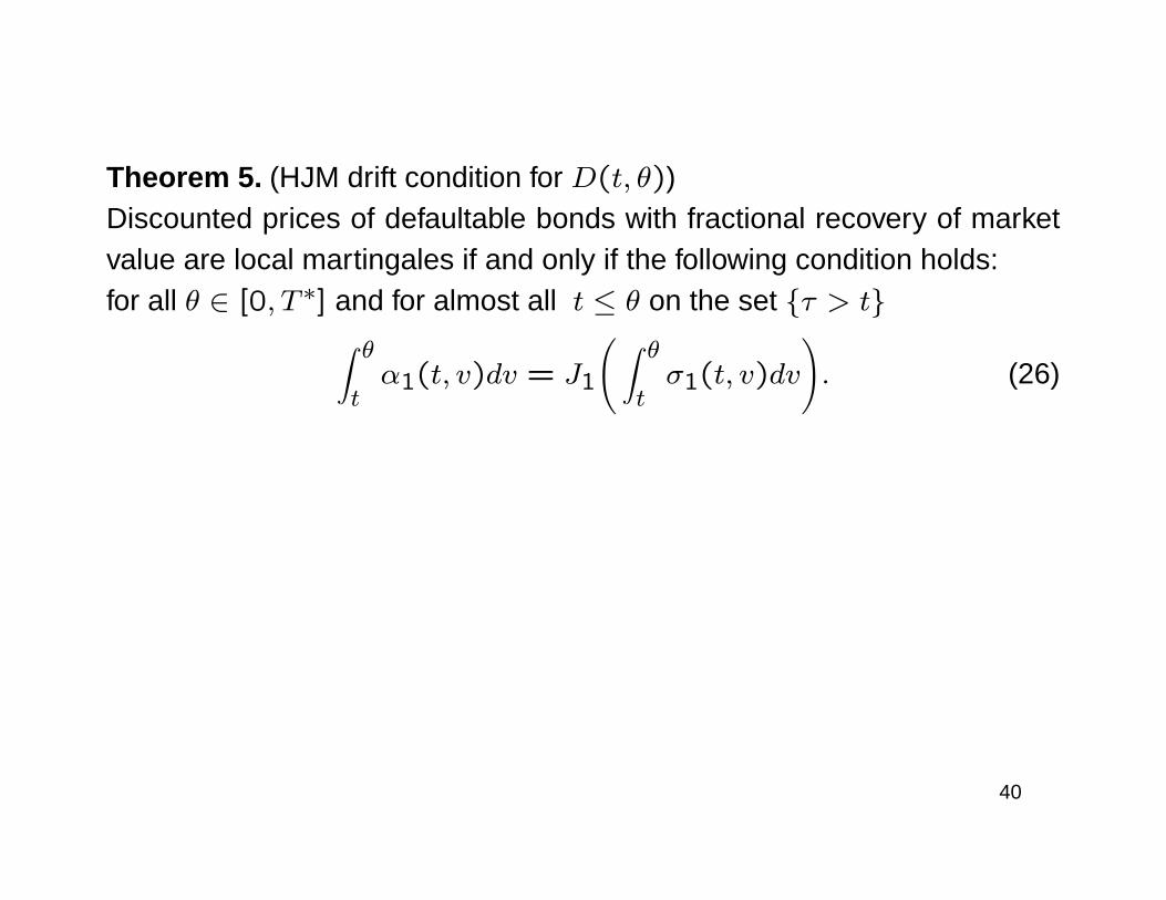
Theorem 5. (HJM drift condition for D(t, θ))Discounted prices of defaultable bonds with fractional recovery of marketvalue are local martingales if and only if the following condition holds:for all θ ∈ [0, T ∗] and for almost all t ≤ θ on the set τ > t∫ θ
tα1(t, v)dv = J1
( ∫ θtσ1(t, v)dv
). (26)
40

Lemma 6. Let τ and Ht be as above and Dt be a process of the form:
Dt = (1−Ht)Xt +HtYt +HtZτ ,
where processes Xt, Yt have local martingale parts MXt and MY
t andabsolutely continuous drifts αXt , α
Yt , which means that processes Xt, Yt
have decompositions:
dXt = αXt dt+ dMXt , dYt = αYt dt+ dMY
t .
Moreover we assume that X and Y have no jumps at τ i.e. ∆Xτ =
∆Yτ = 0. Then Dt is local martingale if and only if for each t ∈ [0, T ]
the following conditions hold:
αXt = λt(Xt− − Yt− − Zt) on the set τ > t (27)
αYt = 0 on the set τ ≤ t (28)
41

• Fractional recovery of treasury
Dδ(θ, θ) = 1τ>θ + 1τ≤θ · δ.
So Dδ(t, θ) = 1τ>te−∫ θt g1(t,u)du + 1τ≤t · δ ·B(t, θ).
Therefore
Dδ(t, θ) = (1−Ht)D1(t, θ) +HtδB(t, θ). (29)
Theorem 7. (HJM drift condition for Dδ(t, θ))The processes of discounted defaultable bond prices with fractional reco-very of treasury are local martingales if and only if the following conditionholds:for all θ ∈ [0, T ∗] and for almost all t ≤ θ on the set τ > t∫ θ
tα1(t, v)dv = J1
( ∫ θtσ1(t, v)dv
)+ δ
(B(t−, θ)D1(t−, θ)
− 1
)λt. (30)
42
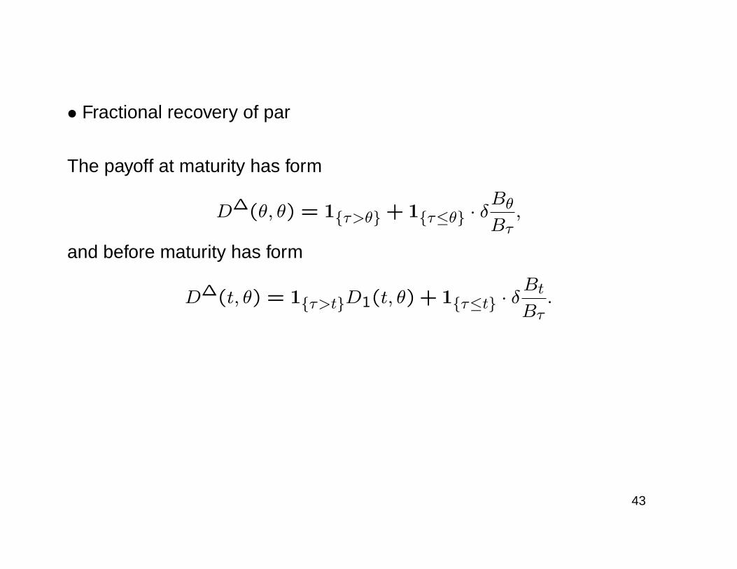
• Fractional recovery of par
The payoff at maturity has form
D∆(θ, θ) = 1τ>θ + 1τ≤θ · δBθBτ,
and before maturity has form
D∆(t, θ) = 1τ>tD1(t, θ) + 1τ≤t · δBt
Bτ.
43
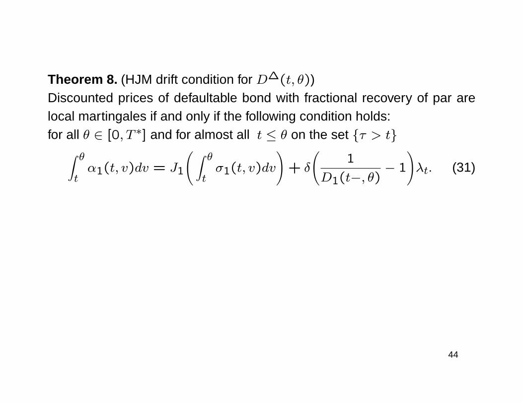
Theorem 8. (HJM drift condition for D∆(t, θ))Discounted prices of defaultable bond with fractional recovery of par arelocal martingales if and only if the following condition holds:for all θ ∈ [0, T ∗] and for almost all t ≤ θ on the set τ > t∫ θ
tα1(t, v)dv = J1
( ∫ θtσ1(t, v)dv
)+ δ
(1
D1(t−, θ)− 1
)λt. (31)
44
• Fractional recovery with multiple defaults
A holder of such defaultable bond receives, at maturity θ,
Dm(θ, θ) =∏τi≤θ
(1− Lτi).
If we introduce process Vt by the formula:
Vt =∏τi≤t
(1− Lτi),
then Dm(θ, θ) = Vθ and for t ≤ θ:
Dm(t, θ) = Vte−∫ θt g1(t,u)du = VtD1(t, θ).
Moreover, we assume that τi are moments of jumps of Cox processNt (do-ubly stochastic Poisson process) with stochastic intensity process (λt)t≥0.It can be shown that Vt solves the following SDE:
dVt = −Vt−LtdNt, (32)
45

and the process
Mt = Nt −∫ t0λudu (33)
follows G - martingale.Theorem 9. Discounted prices of defaultable bonds with multiple defaultsand fractional recovery are local martingales if and only if the followingcondition holds:for all θ ∈ [0, T ∗] and for almost all t ≤ θ on the set Vt− > 0∫ θ
tα1(t, v)dv = J1
( ∫ θtσ1(t, v)dv
). (34)
46
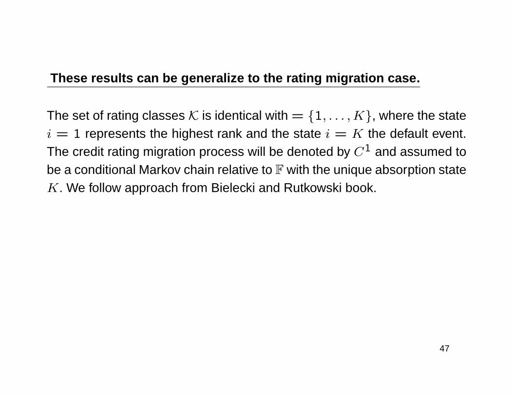
These results can be generalize to the rating migration case.
The set of rating classes K is identical with = 1, . . . ,K, where the statei = 1 represents the highest rank and the state i = K the default event.The credit rating migration process will be denoted by C1 and assumed tobe a conditional Markov chain relative to F with the unique absorption stateK. We follow approach from Bielecki and Rutkowski book.
47
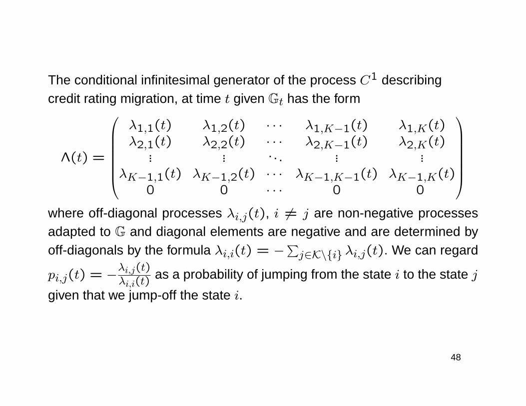
The conditional infinitesimal generator of the process C1 describingcredit rating migration, at time t given Gt has the form
Λ(t) =
λ1,1(t) λ1,2(t) · · · λ1,K−1(t) λ1,K(t)λ2,1(t) λ2,2(t) · · · λ2,K−1(t) λ2,K(t)
... ... . . . ... ...λK−1,1(t) λK−1,2(t) · · · λK−1,K−1(t) λK−1,K(t)
0 0 · · · 0 0
where off-diagonal processes λi,j(t), i 6= j are non-negative processesadapted to G and diagonal elements are negative and are determined byoff-diagonals by the formula λi,i(t) = −
∑j∈K\i λi,j(t). We can regard
pi,j(t) = −λi,j(t)λi,i(t)
as a probability of jumping from the state i to the state j
given that we jump-off the state i.
48

By f we denote the forward process associated with risk free bond andby g1, g2, ..., gK−1 the pre-default term structures associated with ratings1,2, ...,K−1. The pre-default term structure g is thus given by the formula
g(t, u) = gC1(t)(t, u) = 1C1(t)=1g1(t, u) + . . .+
+ 1C1(t)=K−1gK−1(t, u).
To avoid arbitrage it is reasonable to assume that
gK−1(t, θ) > gK−2(t, θ) > . . . > g1(t, θ) > f(t, θ)
for all t ∈ [0, θ] and all θ ∈ [0, T ∗].
48
Hypothesis (H4):
gi(t, t)− f(t, t) = λi,K(t)(1− δi(t)), i = 1, . . . ,K − 1, (35)
so the intensity of migration from rating i into default stateK is equal to theshort term spread for rating i divided by one minus recovery from rating i.Of course, (35) implies
gC1(t)(t, t) = f(t, t) + (1− δC1(t)(t))λC1(t),K(t), (36)
49
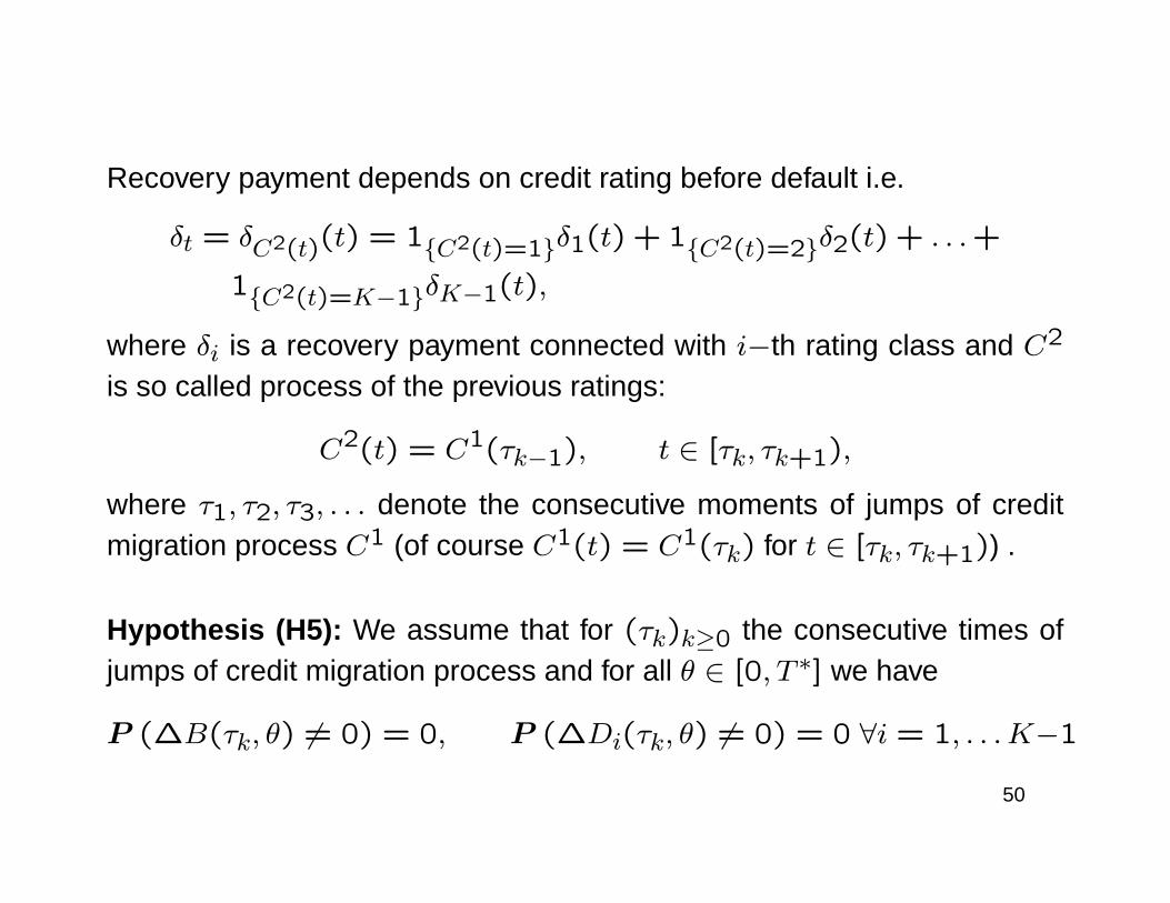
Recovery payment depends on credit rating before default i.e.
δt = δC2(t)(t) = 1C2(t)=1δ1(t) + 1C2(t)=2δ2(t) + . . .+
1C2(t)=K−1δK−1(t),
where δi is a recovery payment connected with i−th rating class and C2
is so called process of the previous ratings:
C2(t) = C1(τk−1), t ∈ [τk, τk+1),
where τ1, τ2, τ3, . . . denote the consecutive moments of jumps of creditmigration process C1 (of course C1(t) = C1(τk) for t ∈ [τk, τk+1)) .
Hypothesis (H5): We assume that for (τk)k≥0 the consecutive times ofjumps of credit migration process and for all θ ∈ [0, T ∗] we have
P (∆B(τk, θ) 6= 0) = 0, P (∆Di(τk, θ) 6= 0) = 0 ∀i = 1, . . .K−1
50
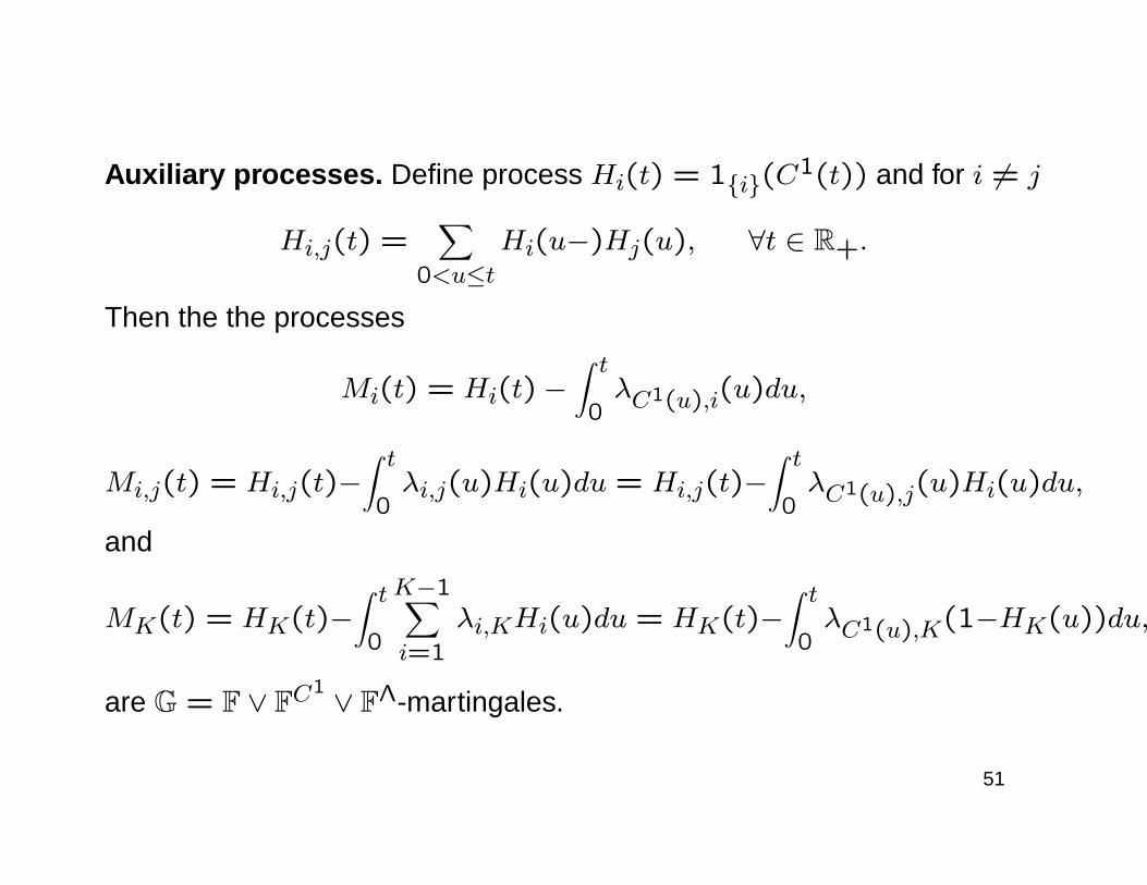
Auxiliary processes. Define process Hi(t) = 1i(C1(t)) and for i 6= j
Hi,j(t) =∑
0<u≤tHi(u−)Hj(u), ∀t ∈ R+.
Then the the processes
Mi(t) = Hi(t)−∫ t0λC1(u),i(u)du,
Mi,j(t) = Hi,j(t)−∫ t0λi,j(u)Hi(u)du = Hi,j(t)−
∫ t0λC1(u),j(u)Hi(u)du,
and
MK(t) = HK(t)−∫ t0
K−1∑i=1
λi,KHi(u)du = HK(t)−∫ t0λC1(u),K(1−HK(u))du,
are G = F ∨ FC1 ∨ FΛ-martingales.
51
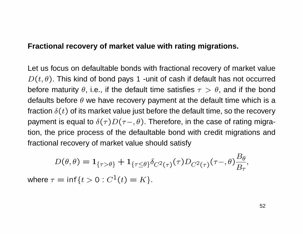
Fractional recovery of market value with rating migrations.
Let us focus on defaultable bonds with fractional recovery of market valueD(t, θ). This kind of bond pays 1 -unit of cash if default has not occurredbefore maturity θ, i.e., if the default time satisfies τ > θ, and if the bonddefaults before θ we have recovery payment at the default time which is afraction δ(t) of its market value just before the default time, so the recoverypayment is equal to δ(τ)D(τ−, θ). Therefore, in the case of rating migra-tion, the price process of the defaultable bond with credit migrations andfractional recovery of market value should satisfy
D(θ, θ) = 1τ>θ + 1τ≤θδC2(τ)(τ)DC2(τ)(τ−, θ)BθBτ,
where τ = inft > 0 : C1(t) = K.
52

Hence we postulate that for t ≤ θ
D(t, θ) = 1C1(t) 6=KDC1(t)(t, θ) +
1C1(t)=KδC2(τ)(τ)DC2(τ)(τ−, θ)Bt
Bτ
=K−1∑i=1
1C1(t) 6=K1C1(t)=iDi(t, θ) +
K−1∑i=1
1C1(t)=K1C2(t)=iδi(τ)Di(τ−, θ)Bt
Bτ
or, equivalently,
D(t, θ) =K−1∑i=1
(Hi(t)Di(t, θ) +Hi,K(t)δi(τ)Di(τ−, θ)
Bt
Bτ
). (37)
53
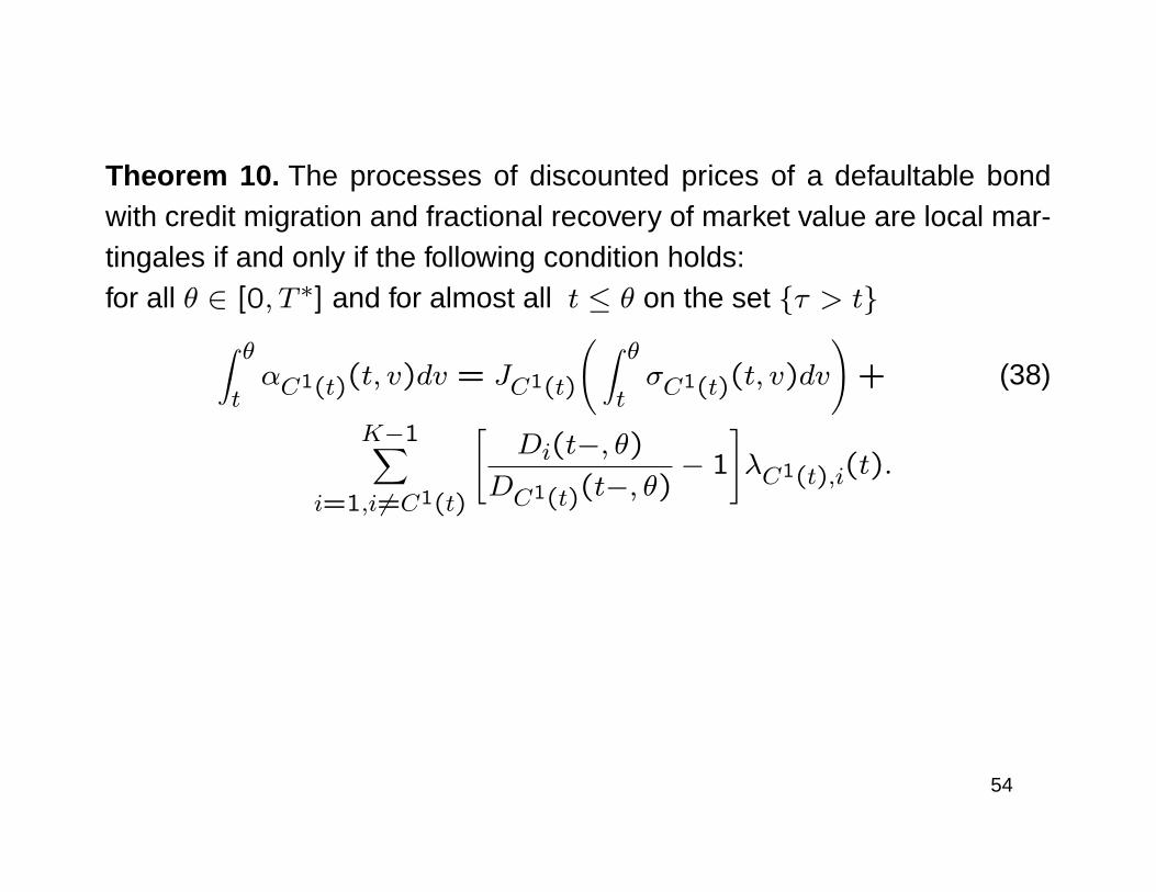
Theorem 10. The processes of discounted prices of a defaultable bondwith credit migration and fractional recovery of market value are local mar-tingales if and only if the following condition holds:for all θ ∈ [0, T ∗] and for almost all t ≤ θ on the set τ > t∫ θ
tαC1(t)(t, v)dv = JC1(t)
( ∫ θtσC1(t)(t, v)dv
)+ (38)
K−1∑i=1,i6=C1(t)
[Di(t−, θ)
DC1(t)(t−, θ)− 1
]λC1(t),i(t).
54
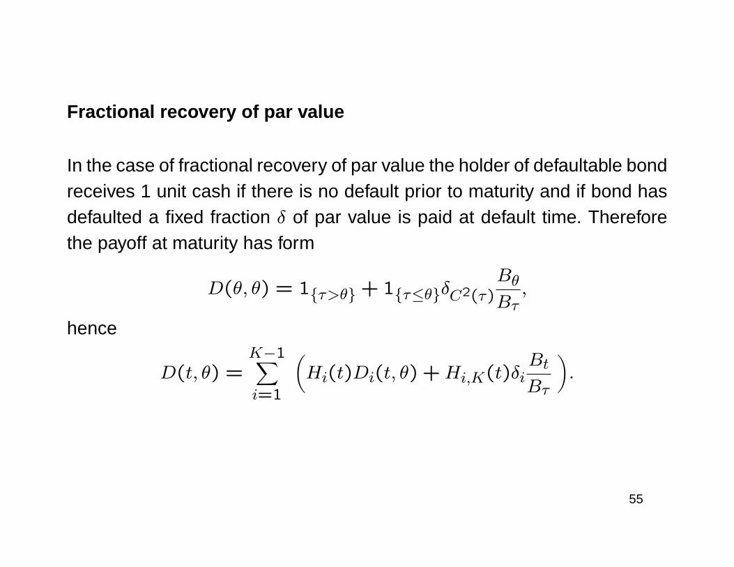
Fractional recovery of par value
In the case of fractional recovery of par value the holder of defaultable bondreceives 1 unit cash if there is no default prior to maturity and if bond hasdefaulted a fixed fraction δ of par value is paid at default time. Thereforethe payoff at maturity has form
D(θ, θ) = 1τ>θ + 1τ≤θδC2(τ)BθBτ,
hence
D(t, θ) =K−1∑i=1
(Hi(t)Di(t, θ) +Hi,K(t)δi
Bt
Bτ
).
55
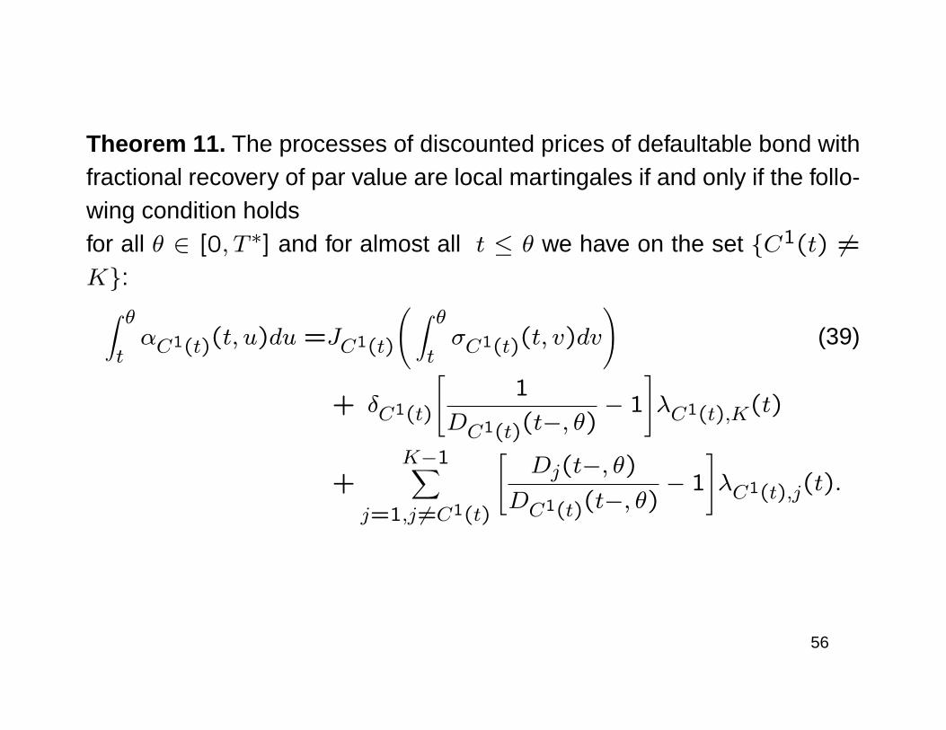
Theorem 11. The processes of discounted prices of defaultable bond withfractional recovery of par value are local martingales if and only if the follo-wing condition holdsfor all θ ∈ [0, T ∗] and for almost all t ≤ θ we have on the set C1(t) 6=K:∫ θ
tαC1(t)(t, u)du =JC1(t)
( ∫ θtσC1(t)(t, v)dv
)(39)
+ δC1(t)
[1
DC1(t)(t−, θ)− 1
]λC1(t),K(t)
+K−1∑
j=1,j 6=C1(t)
[Dj(t−, θ)
DC1(t)(t−, θ)− 1
]λC1(t),j(t).
56
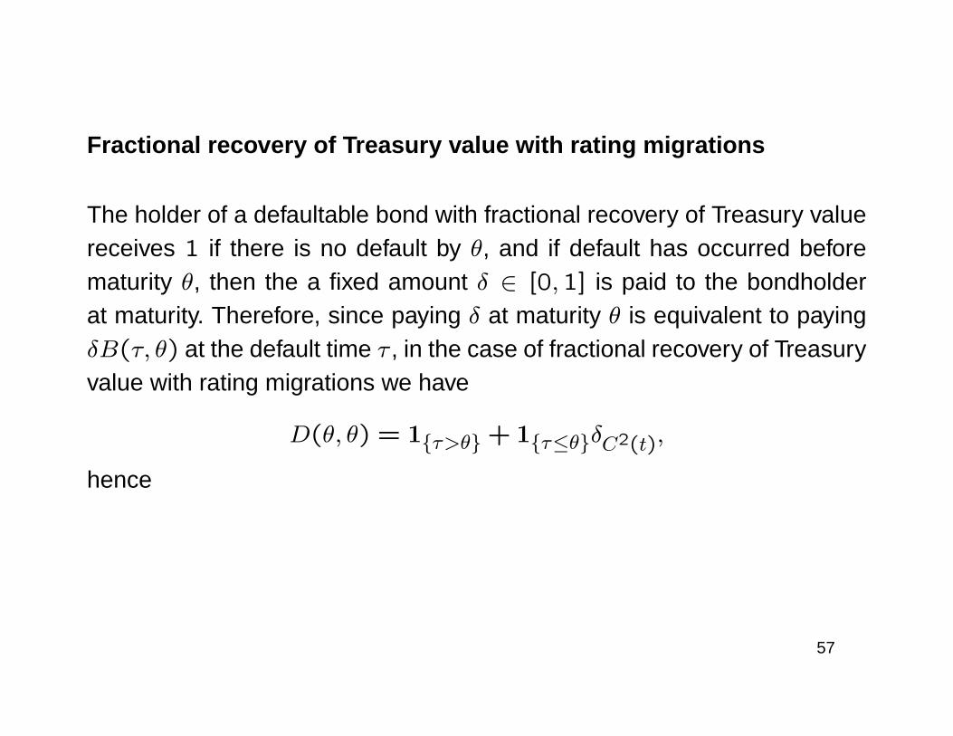
Fractional recovery of Treasury value with rating migrations
The holder of a defaultable bond with fractional recovery of Treasury valuereceives 1 if there is no default by θ, and if default has occurred beforematurity θ, then the a fixed amount δ ∈ [0,1] is paid to the bondholderat maturity. Therefore, since paying δ at maturity θ is equivalent to payingδB(τ, θ) at the default time τ , in the case of fractional recovery of Treasuryvalue with rating migrations we have
D(θ, θ) = 1τ>θ + 1τ≤θδC2(t),
hence
57
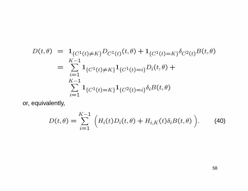
D(t, θ) = 1C1(t) 6=KDC1(t)(t, θ) + 1C1(t)=KδC2(t)B(t, θ)
=K−1∑i=1
1C1(t) 6=K1C1(t)=iDi(t, θ) +
K−1∑i=1
1C1(t)=K1C2(t)=iδiB(t, θ)
or, equivalently,
D(t, θ) =K−1∑i=1
(Hi(t)Di(t, θ) +Hi,K(t)δiB(t, θ)
). (40)
58
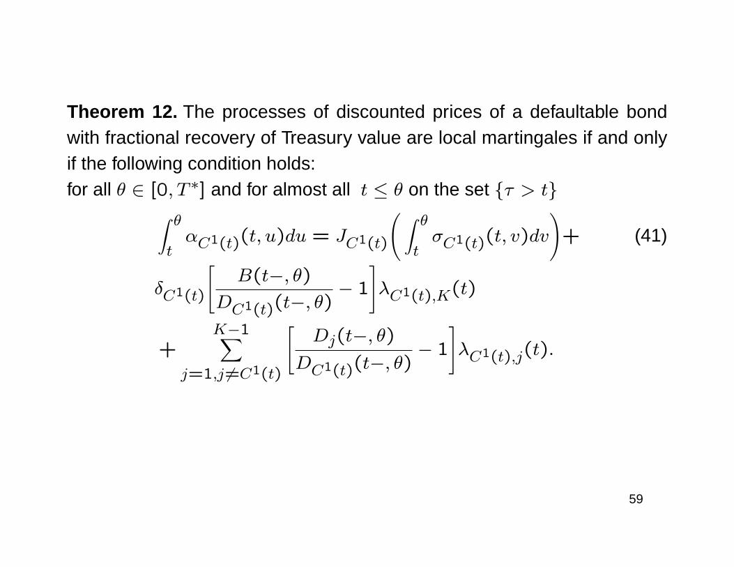
Theorem 12. The processes of discounted prices of a defaultable bondwith fractional recovery of Treasury value are local martingales if and onlyif the following condition holds:for all θ ∈ [0, T ∗] and for almost all t ≤ θ on the set τ > t∫ θ
tαC1(t)(t, u)du = JC1(t)
( ∫ θtσC1(t)(t, v)dv
)+ (41)
δC1(t)
[B(t−, θ)
DC1(t)(t−, θ)− 1
]λC1(t),K(t)
+K−1∑
j=1,j 6=C1(t)
[Dj(t−, θ)
DC1(t)(t−, θ)− 1
]λC1(t),j(t).
59
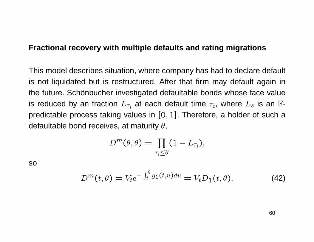
Fractional recovery with multiple defaults and rating migrations
This model describes situation, where company has had to declare defaultis not liquidated but is restructured. After that firm may default again inthe future. Schönbucher investigated defaultable bonds whose face valueis reduced by an fraction Lτi at each default time τi, where Ls is an F-predictable process taking values in [0,1]. Therefore, a holder of such adefaultable bond receives, at maturity θ,
Dm(θ, θ) =∏τi≤θ
(1− Lτi),
so
Dm(t, θ) = Vte−∫ θt g1(t,u)du = VtD1(t, θ). (42)
60
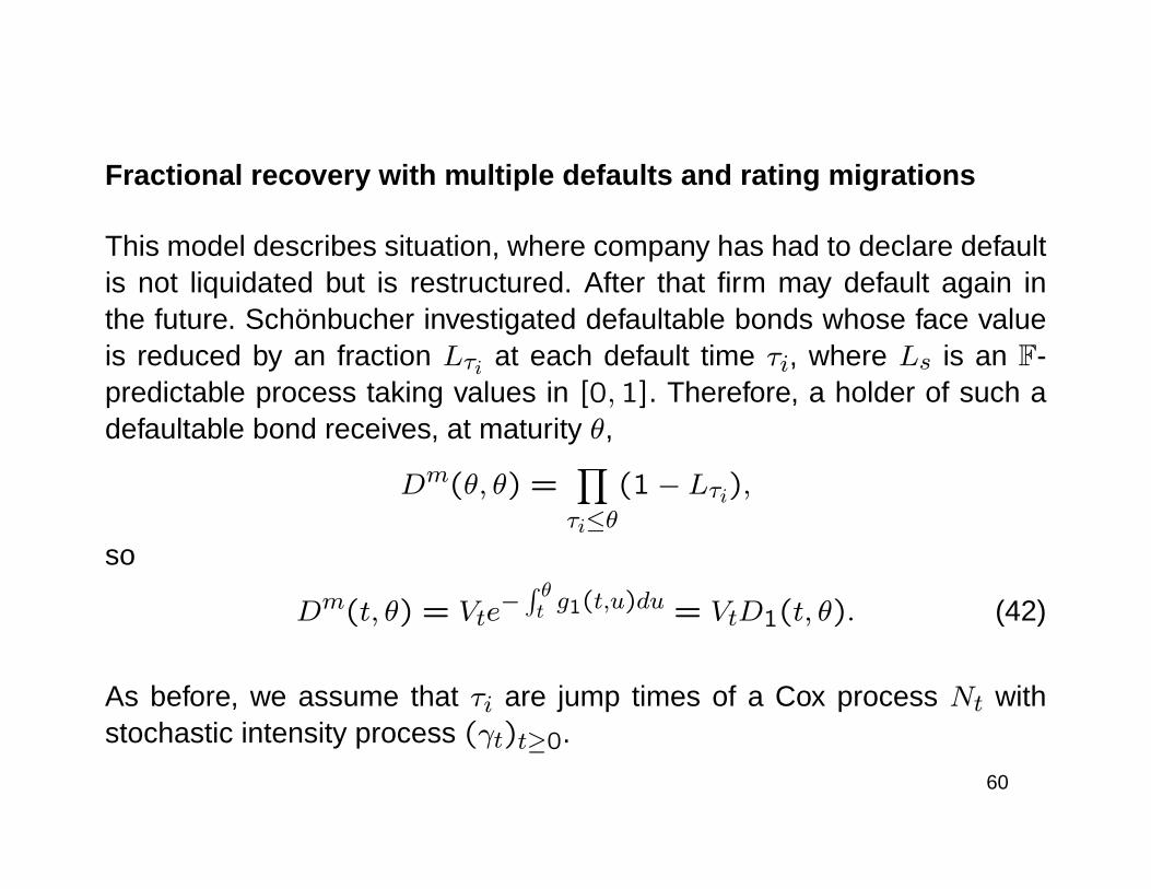
Fractional recovery with multiple defaults and rating migrations
This model describes situation, where company has had to declare defaultis not liquidated but is restructured. After that firm may default again inthe future. Schönbucher investigated defaultable bonds whose face valueis reduced by an fraction Lτi at each default time τi, where Ls is an F-predictable process taking values in [0,1]. Therefore, a holder of such adefaultable bond receives, at maturity θ,
Dm(θ, θ) =∏τi≤θ
(1− Lτi),
so
Dm(t, θ) = Vte−∫ θt g1(t,u)du = VtD1(t, θ). (42)
As before, we assume that τi are jump times of a Cox process Nt withstochastic intensity process (γt)t≥0.
60
We add a rating migration process to the model. Since a company afterdefault is restructured, the rating migration process has no absorbing stateand for the rating migration process C(t) we take a conditional Markovchain with values in the set 1, . . . ,K−1. Moreover, we assume that theprocess describing fractional losses does not depend on the credit migra-tion process.
61
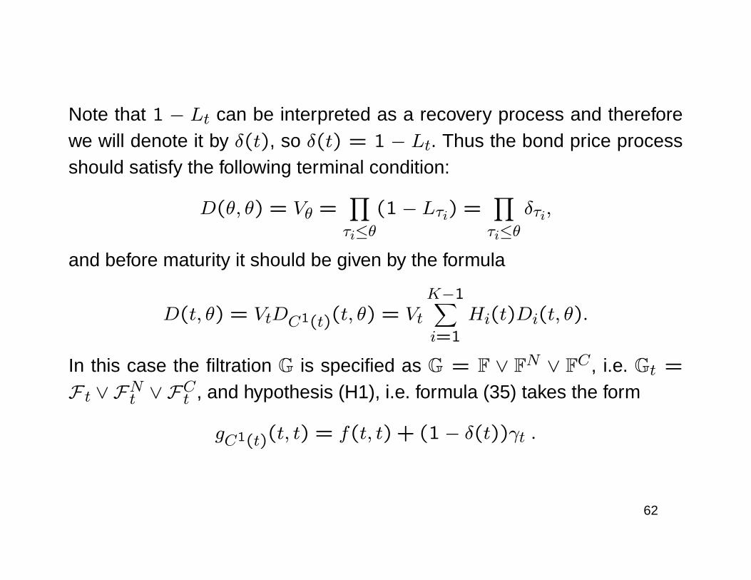
Note that 1 − Lt can be interpreted as a recovery process and thereforewe will denote it by δ(t), so δ(t) = 1 − Lt. Thus the bond price processshould satisfy the following terminal condition:
D(θ, θ) = Vθ =∏τi≤θ
(1− Lτi) =∏τi≤θ
δτi,
and before maturity it should be given by the formula
D(t, θ) = VtDC1(t)(t, θ) = Vt
K−1∑i=1
Hi(t)Di(t, θ).
In this case the filtration G is specified as G = F ∨ FN ∨ FC , i.e. Gt =
F t ∨ FNt ∨ FCt , and hypothesis (H1), i.e. formula (35) takes the form
gC1(t)(t, t) = f(t, t) + (1− δ(t))γt .
62
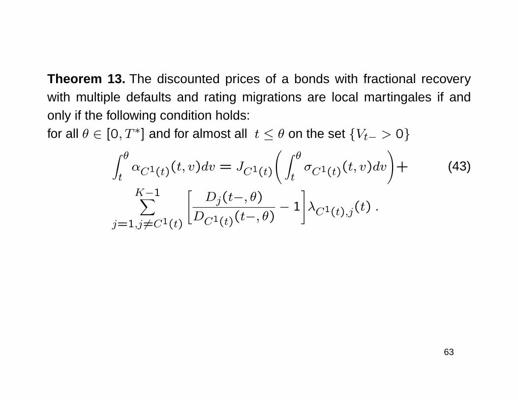
Theorem 13. The discounted prices of a bonds with fractional recoverywith multiple defaults and rating migrations are local martingales if andonly if the following condition holds:for all θ ∈ [0, T ∗] and for almost all t ≤ θ on the set Vt− > 0∫ θ
tαC1(t)(t, v)dv = JC1(t)
( ∫ θtσC1(t)(t, v)dv
)+ (43)
K−1∑j=1,j 6=C1(t)
[Dj(t−, θ)
DC1(t)(t−, θ)− 1
]λC1(t),j(t) .
63
Consistency conditionsBielecki and Rutkowski generalized HJM model to defaultable bonds withratings under consistency conditions. We investigate relationship betweenthe the HJM type conditions and consistency conditions analogous to thatin Bielecki and Rutkowski.
64
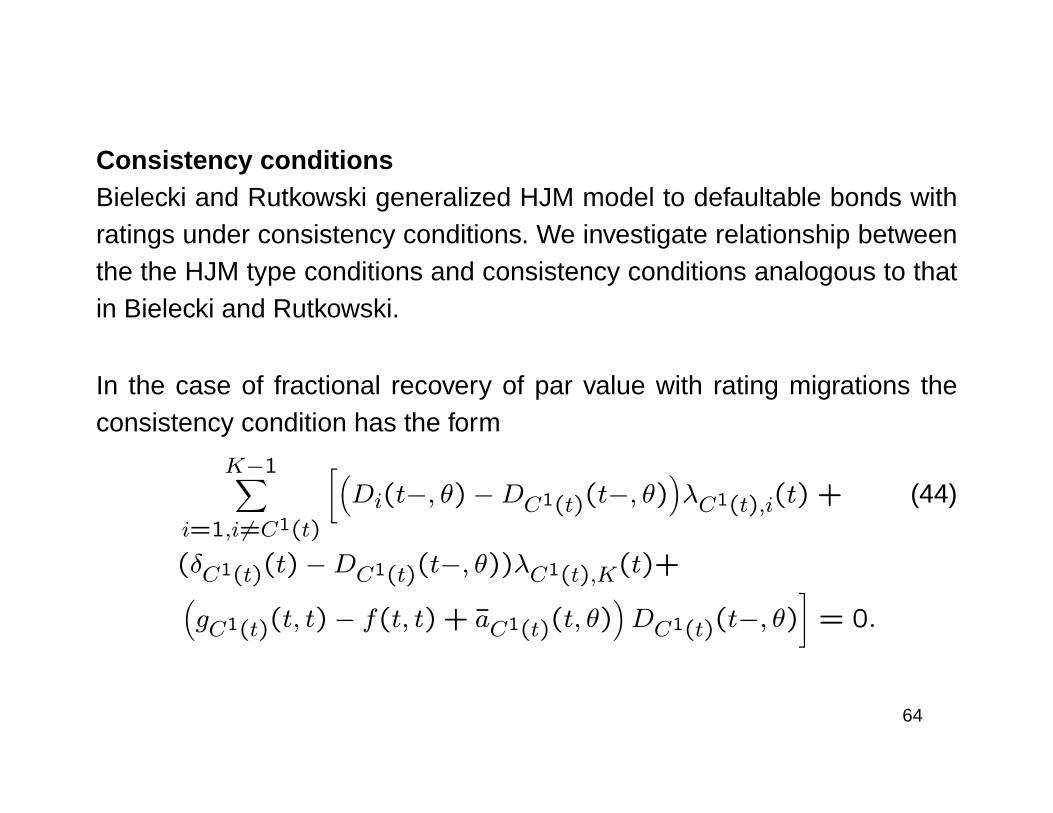
Consistency conditionsBielecki and Rutkowski generalized HJM model to defaultable bonds withratings under consistency conditions. We investigate relationship betweenthe the HJM type conditions and consistency conditions analogous to thatin Bielecki and Rutkowski.
In the case of fractional recovery of par value with rating migrations theconsistency condition has the form
K−1∑i=1,i6=C1(t)
[(Di(t−, θ)−DC1(t)(t−, θ)
)λC1(t),i(t) + (44)
(δC1(t)(t)−DC1(t)(t−, θ))λC1(t),K(t)+(gC1(t)(t, t)− f(t, t) + aC1(t)(t, θ)
)DC1(t)(t−, θ)
]= 0.
64
Theorem 14. For defaultable bonds with fractional recovery of par valuewith rating migration consistency condition (44) holds if and only if HJMtype condition (39) holds.
65

Theorem 14. For defaultable bonds with fractional recovery of par valuewith rating migration consistency condition (44) holds if and only if HJMtype condition (39) holds.
In the case of other kind of recoveries we have very similar situation altho-ugh consistency conditions have slightly different form. So for all kinds ofrecovery
Consistency condition holds if and only if HJM type condition holds.
65
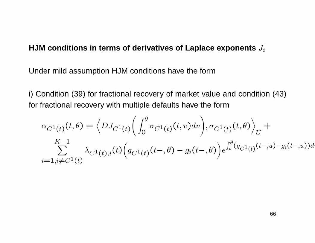
HJM conditions in terms of derivatives of Laplace exponents Ji
Under mild assumption HJM conditions have the form
i) Condition (39) for fractional recovery of market value and condition (43)for fractional recovery with multiple defaults have the form
αC1(t)(t, θ) =⟨DJC1(t)
( ∫ θ0σC1(t)(t, v)dv
), σC1(t)(t, θ)
⟩U
+
K−1∑i=1,i6=C1(t)
λC1(t),i(t)(gC1(t)(t−, θ)− gi(t−, θ)
)e
∫ θt (g
C1(t)(t−,u)−gi(t−,u))du.
66

ii) Condition (41) for fractional recovery of Treasury value has the form
αC1(t)(t, θ) =⟨DJC1(t)
( ∫ θ0σC1(t)(t, v)dv
), σC1(t)(t, θ)
⟩U
+
K−1∑i=1,i6=C1(t)
λC1(t),i(t)(gC1(t)(t−, θ)− gi(t−, θ)
)e
∫ θt (g
C1(t)(t−,u)−gi(t−,u))du
+ δC1(t)λC1(t),K
(gC1(t)(t−, θ)− f(t−, θ)
)e
∫ θt (g
C1(t)(t−,u)−f(t−,u))du.
66
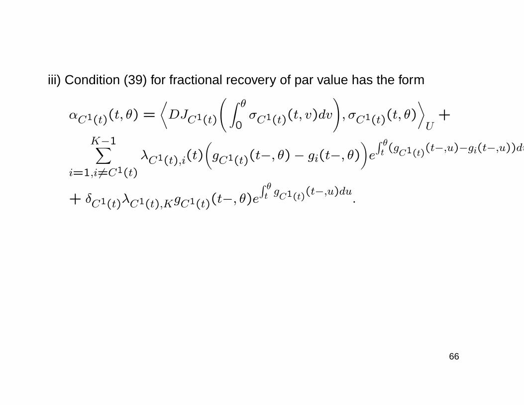
iii) Condition (39) for fractional recovery of par value has the form
αC1(t)(t, θ) =⟨DJC1(t)
( ∫ θ0σC1(t)(t, v)dv
), σC1(t)(t, θ)
⟩U
+
K−1∑i=1,i6=C1(t)
λC1(t),i(t)(gC1(t)(t−, θ)− gi(t−, θ)
)e
∫ θt (g
C1(t)(t−,u)−gi(t−,u))du
+ δC1(t)λC1(t),KgC1(t)(t−, θ)e∫ θt gC1(t)(t−,u)du.
66
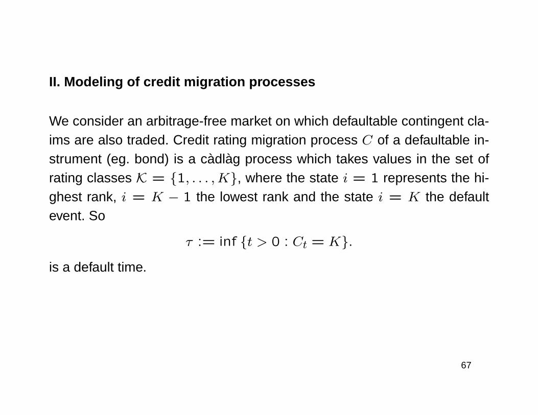
II. Modeling of credit migration processes
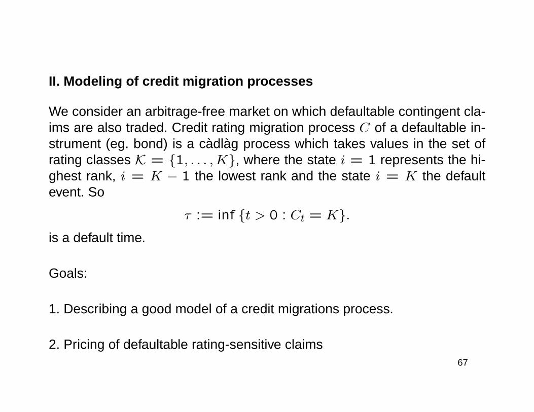
We consider an arbitrage-free market on which defaultable contingent cla-ims are also traded. Credit rating migration process C of a defaultable in-strument (eg. bond) is a càdlàg process which takes values in the set ofrating classes K = 1, . . . ,K, where the state i = 1 represents the hi-ghest rank, i = K − 1 the lowest rank and the state i = K the defaultevent. So
τ := inf t > 0 : Ct = K.
is a default time.
67
II. Modeling of credit migration processes
We consider an arbitrage-free market on which defaultable contingent cla-ims are also traded. Credit rating migration process C of a defaultable in-strument (eg. bond) is a càdlàg process which takes values in the set ofrating classes K = 1, . . . ,K, where the state i = 1 represents the hi-ghest rank, i = K − 1 the lowest rank and the state i = K the defaultevent. So
τ := inf t > 0 : Ct = K.
is a default time.
Goals:
1. Describing a good model of a credit migrations process.
2. Pricing of defaultable rating-sensitive claims67

Doubly Stochastic Markov Chains We assume that all processes are defined
on a complete probability space (Ω,F ,P). We also fix a filtration F, which plays a role
of reference filtration (corresponding to observation of market without credit rating i.e.
filtration corresponding to interest rate risk and other market factors that drives credit
risk).
68

Doubly Stochastic Markov Chains We assume that all processes are defined
on a complete probability space (Ω,F ,P). We also fix a filtration F, which plays a role
of reference filtration (corresponding to observation of market without credit rating i.e.
filtration corresponding to interest rate risk and other market factors that drives credit
risk).
Definition 2. A càdlàg process C is called the F–doubly stochastic Markovchain with state space K ⊂ . . . ,−1,0,1,2, . . . if there exists a family ofstochastic matrices P (s, t) = (pi,j(s, t))i,j∈K for 0 ≤ s ≤ t such that
1. a matrix P (s, t) is Ft measurable, P (s, ·) is progressively measurable
2. for all i, j ∈ K, s ≤ t
P(Ct = j|F∞ ∨ FCs )1Cs=i = 1Cs=ipi,j(s, t). (45)
68
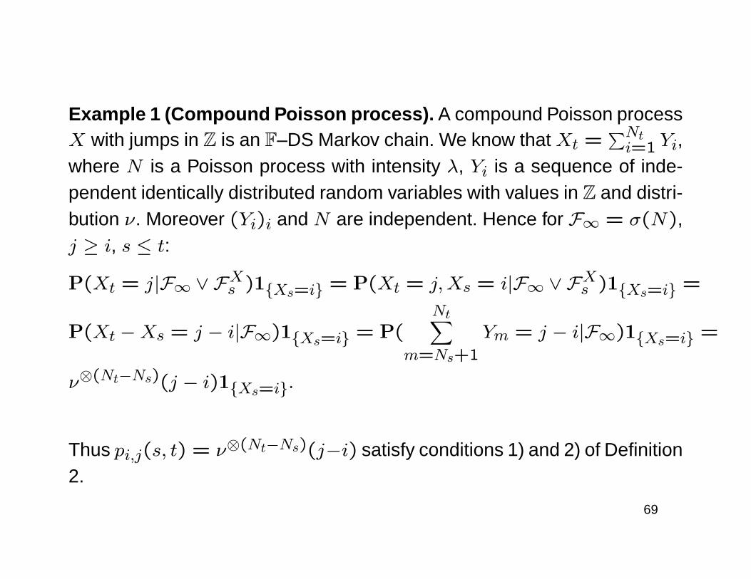
Example 1 (Compound Poisson process). A compound Poisson processX with jumps in Z is an F–DS Markov chain. We know that Xt =
∑Nti=1 Yi,
where N is a Poisson process with intensity λ, Yi is a sequence of inde-pendent identically distributed random variables with values in Z and distri-bution ν. Moreover (Yi)i and N are independent. Hence for F∞ = σ(N),j ≥ i, s ≤ t:
P(Xt = j|F∞ ∨ FXs )1Xs=i = P(Xt = j,Xs = i|F∞ ∨ FXs )1Xs=i =
P(Xt −Xs = j − i|F∞)1Xs=i = P(Nt∑
m=Ns+1
Ym = j − i|F∞)1Xs=i =
ν⊗(Nt−Ns)(j − i)1Xs=i.
Thus pi,j(s, t) = ν⊗(Nt−Ns)(j−i) satisfy conditions 1) and 2) of Definition2.
69
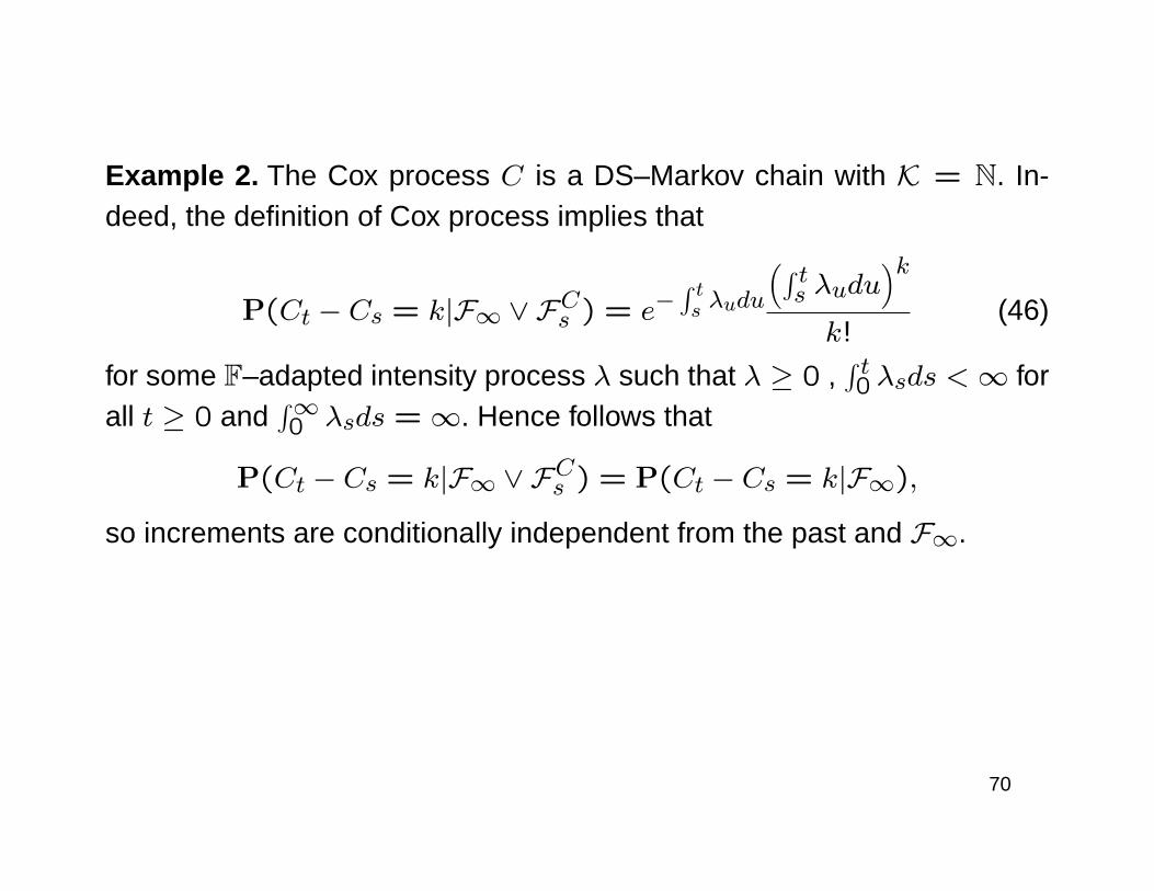
Example 2. The Cox process C is a DS–Markov chain with K = N. In-deed, the definition of Cox process implies that
P(Ct − Cs = k|F∞ ∨ FCs ) = e−∫ ts λudu
(∫ ts λudu
)kk!
(46)
for some F–adapted intensity process λ such that λ ≥ 0 ,∫ t0 λsds <∞ for
all t ≥ 0 and∫∞0 λsds = ∞. Hence follows that
P(Ct − Cs = k|F∞ ∨ FCs ) = P(Ct − Cs = k|F∞),
so increments are conditionally independent from the past and F∞.
70
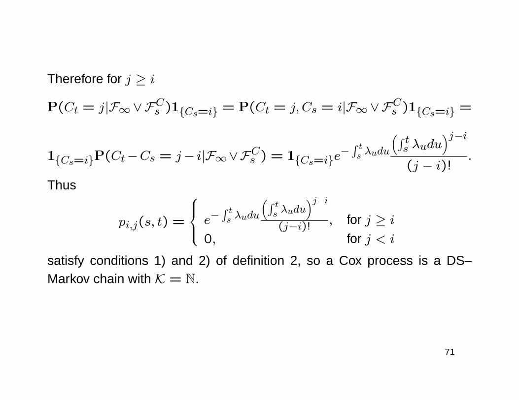
Therefore for j ≥ i
P(Ct = j|F∞∨FCs )1Cs=i = P(Ct = j, Cs = i|F∞∨FCs )1Cs=i =
1Cs=iP(Ct−Cs = j− i|F∞∨FCs ) = 1Cs=ie−∫ ts λudu
(∫ ts λudu
)j−i(j − i)!
.
Thus
pi,j(s, t) =
e−∫ ts λudu
(∫ ts λudu
)j−i(j−i)! , for j ≥ i
0, for j < i
satisfy conditions 1) and 2) of definition 2, so a Cox process is a DS–Markov chain with K = N.
71
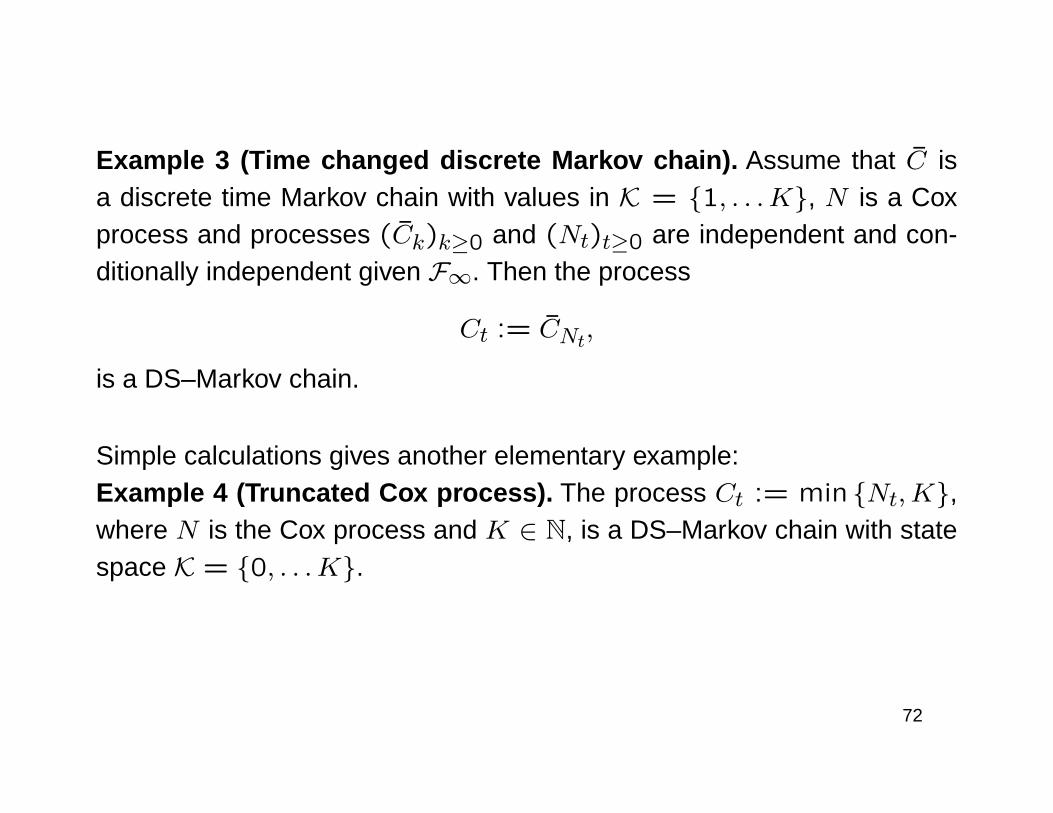
Example 3 (Time changed discrete Markov chain). Assume that C isa discrete time Markov chain with values in K = 1, . . .K, N is a Coxprocess and processes (Ck)k≥0 and (Nt)t≥0 are independent and con-ditionally independent given F∞. Then the process
Ct := CNt,
is a DS–Markov chain.
Simple calculations gives another elementary example:Example 4 (Truncated Cox process). The process Ct := min Nt,K,where N is the Cox process and K ∈ N, is a DS–Markov chain with statespace K = 0, . . .K.
72
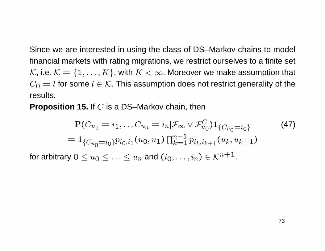
Since we are interested in using the class of DS–Markov chains to modelfinancial markets with rating migrations, we restrict ourselves to a finite setK, i.e. K = 1, . . . ,K, with K <∞. Moreover we make assumption thatC0 = l for some l ∈ K. This assumption does not restrict generality of theresults.Proposition 15. If C is a DS–Markov chain, then
P(Cu1 = i1, . . . Cun = in|F∞ ∨ FCu0)1Cu0=i0 (47)
= 1Cu0=i0pi0,i1(u0, u1)∏n−1k=1 pik,ik+1
(uk, uk+1)
for arbitrary 0 ≤ u0 ≤ . . . ≤ un and (i0, . . . , in) ∈ Kn+1.
73
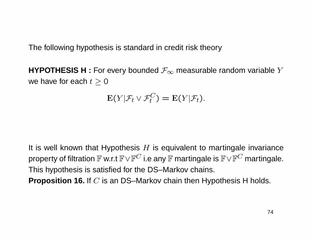
The following hypothesis is standard in credit risk theory
HYPOTHESIS H : For every bounded F∞ measurable random variable Ywe have for each t ≥ 0
E(Y |Ft ∨ FCt ) = E(Y |Ft).
It is well known that Hypothesis H is equivalent to martingale invarianceproperty of filtration F w.r.t F∨FC i.e any F martingale is F∨FC martingale.This hypothesis is satisfied for the DS–Markov chains.Proposition 16. If C is an DS–Markov chain then Hypothesis H holds.
74
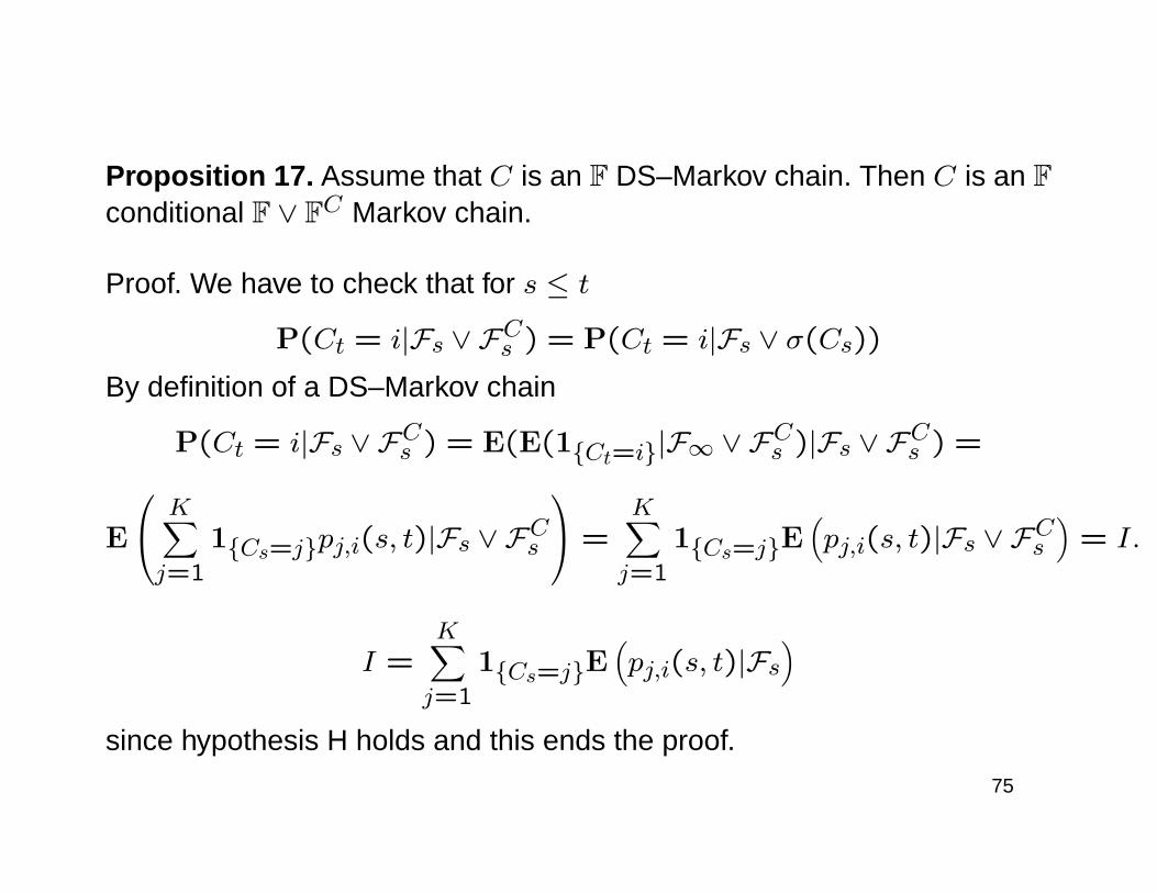
Proposition 17. Assume that C is an F DS–Markov chain. Then C is an Fconditional F ∨ FC Markov chain.
Proof. We have to check that for s ≤ t
P(Ct = i|Fs ∨ FCs ) = P(Ct = i|Fs ∨ σ(Cs))By definition of a DS–Markov chain
P(Ct = i|Fs ∨ FCs ) = E(E(1Ct=i|F∞ ∨ FCs )|Fs ∨ FCs ) =
E
K∑j=1
1Cs=jpj,i(s, t)|Fs ∨ FCs
=K∑j=1
1Cs=jE(pj,i(s, t)|Fs ∨ FCs
)= I.
I =K∑j=1
1Cs=jE(pj,i(s, t)|Fs
)since hypothesis H holds and this ends the proof.
75
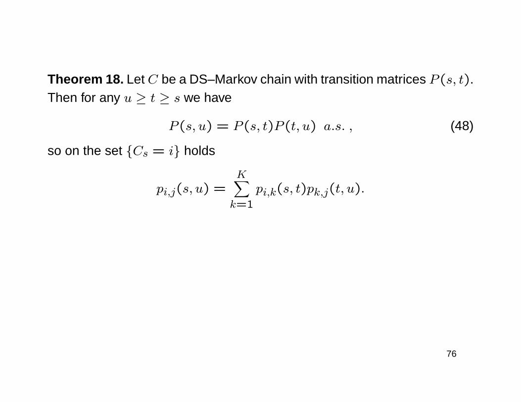
Theorem 18. Let C be a DS–Markov chain with transition matrices P (s, t).Then for any u ≥ t ≥ s we have
P (s, u) = P (s, t)P (t, u) a.s. , (48)
so on the set Cs = i holds
pi,j(s, u) =K∑k=1
pi,k(s, t)pk,j(t, u).
76
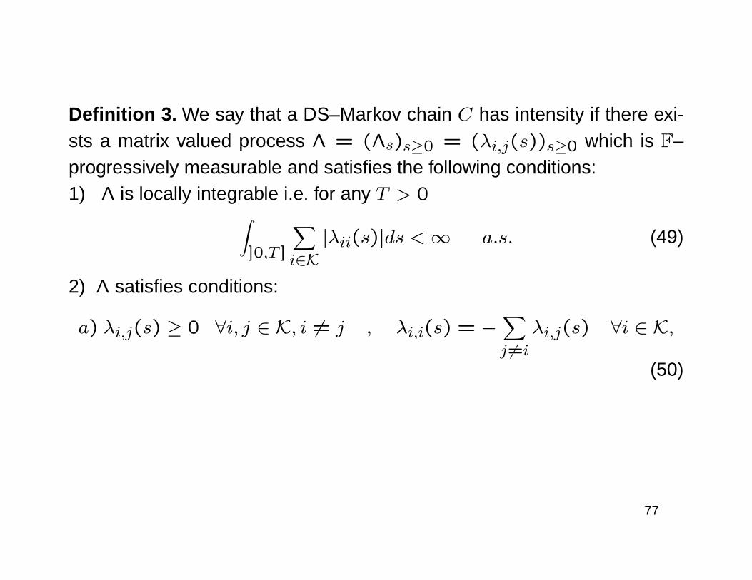
Definition 3. We say that a DS–Markov chain C has intensity if there exi-sts a matrix valued process Λ = (Λs)s≥0 = (λi,j(s))s≥0 which is F–progressively measurable and satisfies the following conditions:1) Λ is locally integrable i.e. for any T > 0∫
]0,T ]
∑i∈K
|λii(s)|ds <∞ a.s. (49)
2) Λ satisfies conditions:
a) λi,j(s) ≥ 0 ∀i, j ∈ K, i 6= j , λi,i(s) = −∑j 6=i
λi,j(s) ∀i ∈ K,
(50)
77
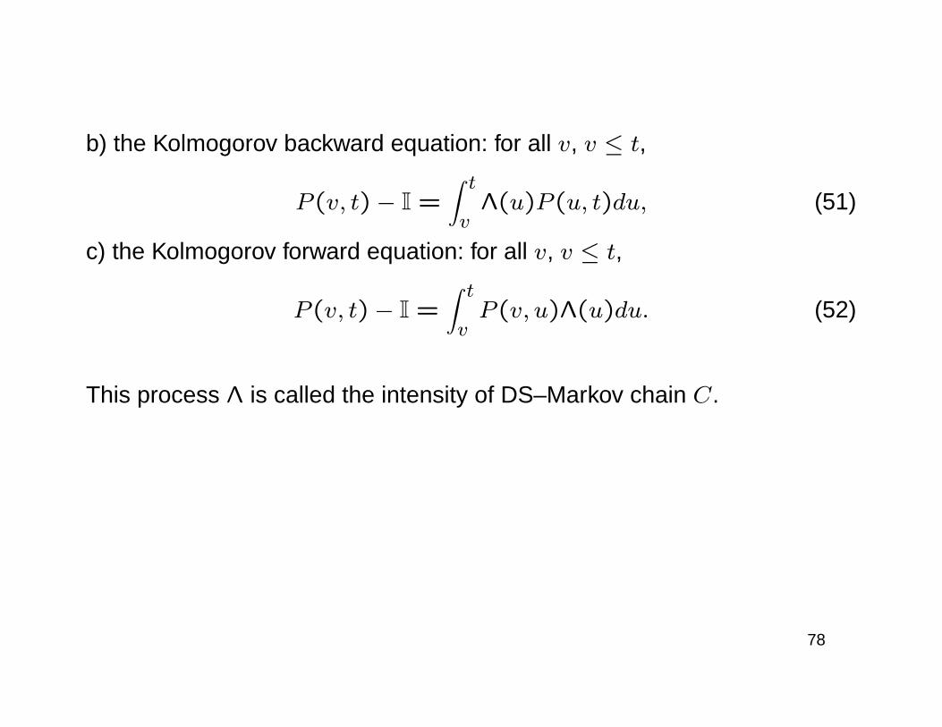
b) the Kolmogorov backward equation: for all v, v ≤ t,
P (v, t)− I =∫ tv
Λ(u)P (u, t)du, (51)
c) the Kolmogorov forward equation: for all v, v ≤ t,
P (v, t)− I =∫ tvP (v, u)Λ(u)du. (52)
This process Λ is called the intensity of DS–Markov chain C.
78

Theorem 19 (Existence of Intensity). Let C be a DS–Markov chain. As-sume that
1. P as a matrix value mapping is measurable i.e.P : (R+ × R+ ×Ω,B(R+ ×R+)⊗F) → (RK×K,B(RK×K)).
2. There exists a version of process P which is continuous in (s, t).
3. For every t ≥ 0 the following limit exists in almost sure sense:
Λt := limh↓0
P (t, t+ h)− Ih
, (53)
and is locally integrable.
Then Λ is the intensity of C.
79

Example 5. If Ct = min Nt,K, where N is a Cox process with intensityprocess λ, then C has the intensity process of the following form
λi,j(t) =
−λ(t), for i = j ∈ 0, . . .K − 1;λ(t), for j = i+ 1 with i ∈ 0, . . .K − 1;0, otherwise.
Example 6. If Ct = CNt, then Λ given by
λi,j(t) = (P − I)i,jλt
is the intensity of C.
80
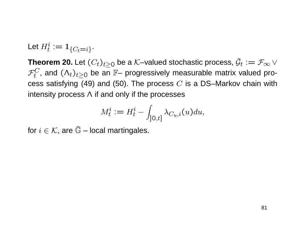
Let Hit := 1Ct=i.
Theorem 20. Let (Ct)t≥0 be a K–valued stochastic process, Gt := F∞ ∨FCt , and (Λt)t≥0 be an F– progressively measurable matrix valued pro-cess satisfying (49) and (50). The process C is a DS–Markov chain withintensity process Λ if and only if the processes
M it := Hi
t −∫]0,t]
λCu,i(u)du,
for i ∈ K, are G – local martingales.
81

Theorem 21. The processes M i for all i ∈ K are local martingales if andonly if the processes
Mi,jt := H
i,jt −
∫]0,t]
Hisλi,j(s)ds,
where
Hi,jt :=
∫]0,t]
Hiu−dH
ju (54)
are local martingales for i 6= j ∈ K.
Processes Hi,j defined by (54) counts number of jumps from state i to jup to time t, one can show that
Hi,j =∑
0<u≤tHiu−H
ju.
82

Since M i are adapted to G with Gt = Ft ∨FCt , which is sub-filtration of Gwe have:Corollary 3. If C is Doubly Stochastic Markov Process, then M i are Glocal martingales.
Remark 6. Process C obtained by the canonical construction in BieleckiRutkowski book is a DS–Markov chain. This is a consequence of theorem20, because calculations analogous to lemma 11.3.2 page 347 shows thatM i are G martingales and in the canonical construction Λ is bounded.
83

Since M i are adapted to G with Gt = Ft ∨FCt , which is sub-filtration of Gwe have:Corollary 3. If C is Doubly Stochastic Markov Process, then M i are Glocal martingales.
Remark 6. Process C obtained by the canonical construction in BieleckiRutkowski book is a DS–Markov chain. This is a consequence of theorem20, because calculations analogous to lemma 11.3.2 page 347 shows thatM i are G martingales and in the canonical construction Λ is bounded.
Theorem 22. Let (Λt)t≥0 be an arbitrary locally integrable F– progressi-vely measurable matrix valued process which satisfies condition (50). Thenwe can construct DS–Markov chain with intensity (Λt)t≥0 and given initialstate i0.
83
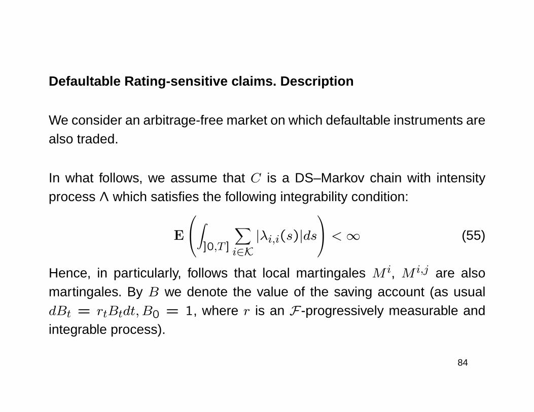
Defaultable Rating-sensitive claims. Description
We consider an arbitrage-free market on which defaultable instruments arealso traded.
In what follows, we assume that C is a DS–Markov chain with intensityprocess Λ which satisfies the following integrability condition:
E
∫]0,T ]
∑i∈K
|λi,i(s)|ds
<∞ (55)
Hence, in particularly, follows that local martingales M i, M i,j are alsomartingales. By B we denote the value of the saving account (as usualdBt = rtBtdt, B0 = 1, where r is an F -progressively measurable andintegrable process).
84
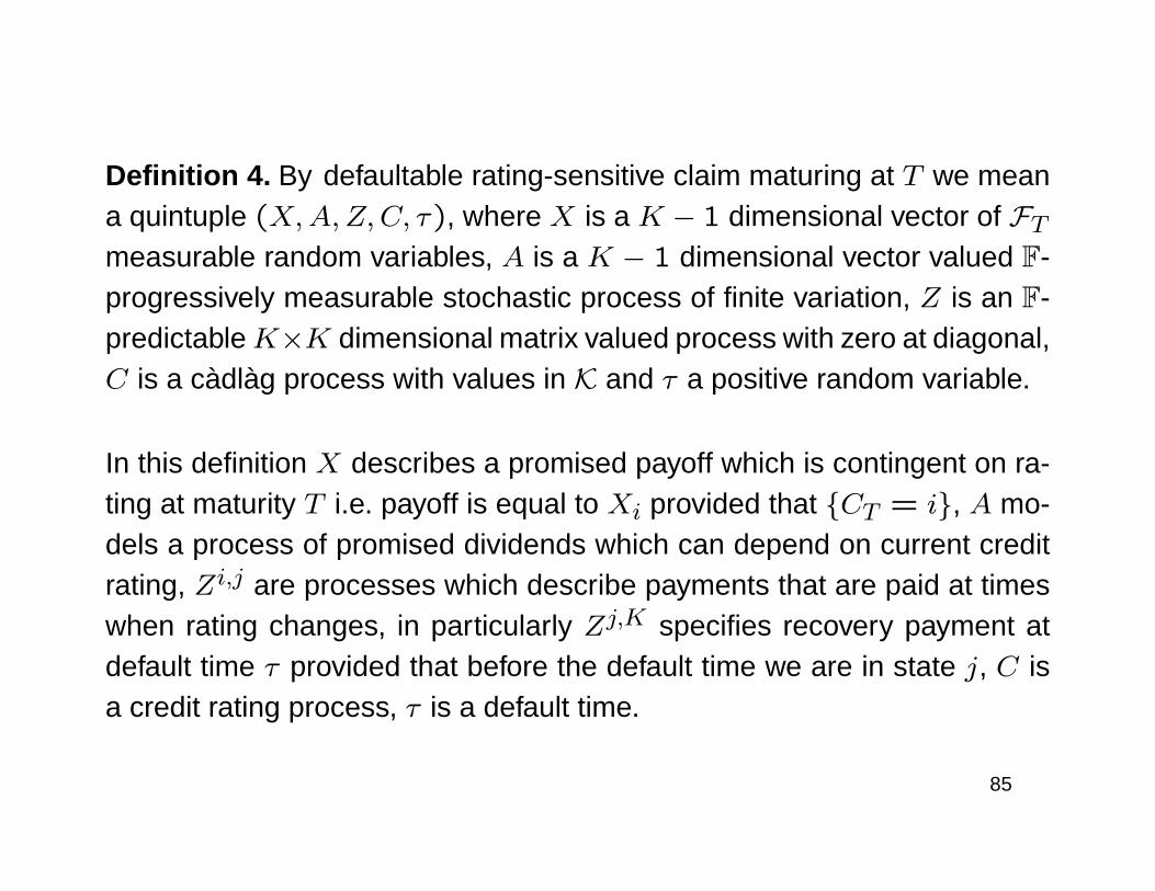
Definition 4. By defaultable rating-sensitive claim maturing at T we meana quintuple (X,A,Z,C, τ), where X is a K − 1 dimensional vector of FTmeasurable random variables, A is a K − 1 dimensional vector valued F-progressively measurable stochastic process of finite variation, Z is an F-predictableK×K dimensional matrix valued process with zero at diagonal,C is a càdlàg process with values in K and τ a positive random variable.
In this definition X describes a promised payoff which is contingent on ra-ting at maturity T i.e. payoff is equal to Xi provided that CT = i, A mo-dels a process of promised dividends which can depend on current creditrating, Zi,j are processes which describe payments that are paid at timeswhen rating changes, in particularly Zj,K specifies recovery payment atdefault time τ provided that before the default time we are in state j, C isa credit rating process, τ is a default time.
85

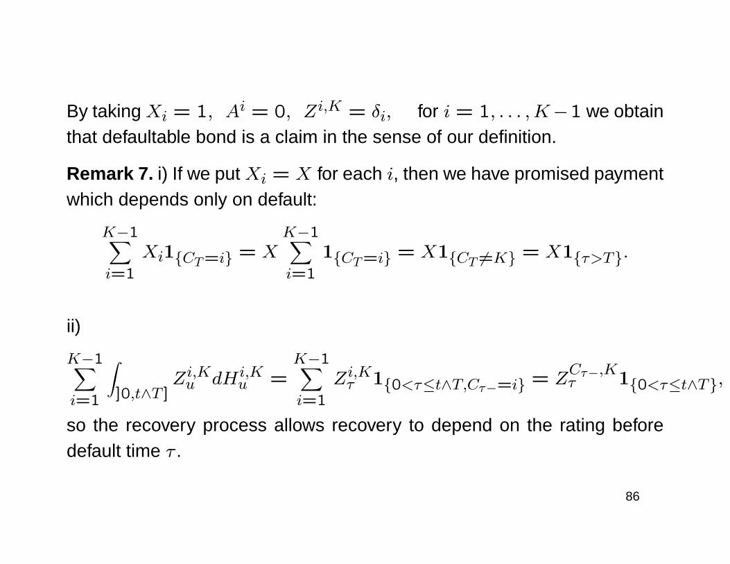
By taking Xi = 1, Ai = 0, Zi,K = δi, for i = 1, . . . ,K−1 we obtainthat defaultable bond is a claim in the sense of our definition.
86

By taking Xi = 1, Ai = 0, Zi,K = δi, for i = 1, . . . ,K−1 we obtainthat defaultable bond is a claim in the sense of our definition.
Remark 7. i) If we put Xi = X for each i, then we have promised paymentwhich depends only on default:
K−1∑i=1
Xi1CT=i = XK−1∑i=1
1CT=i = X1CT 6=K = X1τ>T.
86
By taking Xi = 1, Ai = 0, Zi,K = δi, for i = 1, . . . ,K−1 we obtainthat defaultable bond is a claim in the sense of our definition.
Remark 7. i) If we put Xi = X for each i, then we have promised paymentwhich depends only on default:
K−1∑i=1
Xi1CT=i = XK−1∑i=1
1CT=i = X1CT 6=K = X1τ>T.
ii)
K−1∑i=1
∫]0,t∧T ]
Zi,Ku dHi,Ku =
K−1∑i=1
Zi,Kτ 10<τ≤t∧T,Cτ−=i = ZCτ−,Kτ 10<τ≤t∧T,
so the recovery process allows recovery to depend on the rating beforedefault time τ .
86

Now, we defined the dividend process which describes cash flows fromclaim on the interval [0, T ].
Definition 5. Dividend process D = (Dt)t≥0 of claim (X,A,Z,C, τ) ma-turing at T equals for t ≥ 0
Dt =K−1∑i=1
(XiHiT1[T,+∞[(t) +
∫]0,t∧T ]
HiudA
iu +
∑j 6=i∈K
∫]0,t∧T ]
Zi,ju dHi,ju ).
87

Now, we defined the dividend process which describes cash flows fromclaim on the interval [0, T ].
Definition 5. Dividend process D = (Dt)t≥0 of claim (X,A,Z,C, τ) ma-turing at T equals for t ≥ 0
Dt =K−1∑i=1
(XiHiT1[T,+∞[(t) +
∫]0,t∧T ]
HiudA
iu +
∑j 6=i∈K
∫]0,t∧T ]
Zi,ju dHi,ju ).
Example. The dividend process for defaultable bond equals
Dt = 1τ>T1[T,+∞[(t) + δCτ−10<τ≤t∧T.
87

Example 7 (credit sensitive note ). The coupons of this note are paid atpre-specified coupon dates 0 < T1 < T2 < . . . < Tn, and value of co-upon is contingent on rating corporate at coupon date. Recovery paymentdepends on pre-default rating Cτ−, and it is assumed that δi ∈ [0,1) isfixed for each i ∈ K \K. So
Xi = 1, Zi,K = δi, F = 0, Ait =n∑
j=1
1t≥Tjdi,j,
where di,j are fixed constants chosen in advance and dividend process ofthis note is given by
Dt = 1τ>T1[T,+∞[(t)+K−1∑i=1
∫]0,t∧T ]
δidHi,Ku +
K−1∑i=1
∫]0,t∧T ]
HiudA
iu.
88
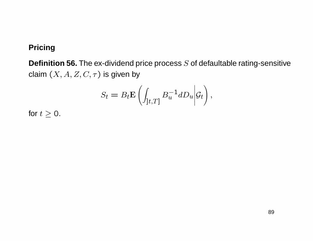
Pricing
Definition 56. The ex-dividend price process S of defaultable rating-sensitiveclaim (X,A,Z,C, τ) is given by
St = BtE
(∫]t,T ]
B−1u dDu
∣∣∣∣∣Gt),
for t ≥ 0.
89
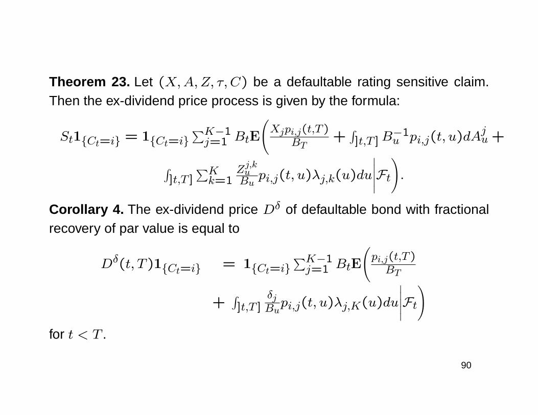
Theorem 23. Let (X,A,Z, τ, C) be a defaultable rating sensitive claim.Then the ex-dividend price process is given by the formula:
St1Ct=i = 1Ct=i∑K−1j=1 BtE
(Xjpi,j(t,T )
BT+∫]t,T ]B
−1u pi,j(t, u)dA
ju +
∫]t,T ]
∑Kk=1
Zj,kuBu
pi,j(t, u)λj,k(u)du
∣∣∣∣∣Ft).
Corollary 4. The ex-dividend price Dδ of defaultable bond with fractionalrecovery of par value is equal to
Dδ(t, T )1Ct=i = 1Ct=i∑K−1j=1 BtE
(pi,j(t,T )BT
+∫]t,T ]
δjBupi,j(t, u)λj,K(u)du
∣∣∣∣∣Ft)
for t < T .
90

Corollary 5. The ex-dividend price of the Credit Sensitive Note with co-upons with resetting at coupon payment date equals
BtE
∑k:t<Tk
dCTk
1τ>TkBTk
∣∣∣∣∣Ft 1Ct=i
= 1Ct=iE
∑k:t<Tk
e−∫ Tkt rudu
K−1∑j=1
djpi,j(t, Tk)
∣∣∣∣∣Ft ,
for t < T .
91
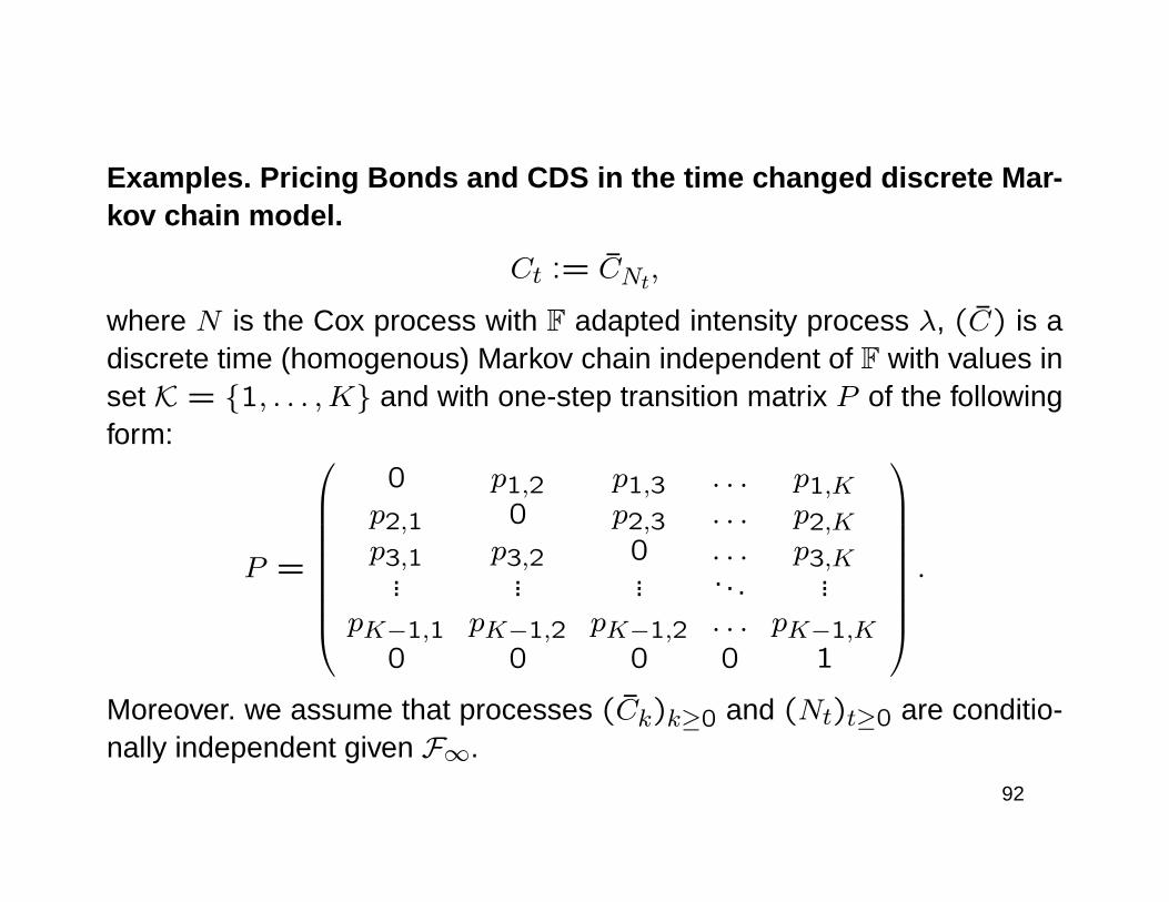
Examples. Pricing Bonds and CDS in the time changed discrete Mar-kov chain model.
Ct := CNt,
where N is the Cox process with F adapted intensity process λ, (C) is adiscrete time (homogenous) Markov chain independent of F with values inset K = 1, . . . ,K and with one-step transition matrix P of the followingform:
P =
0 p1,2 p1,3 . . . p1,Kp2,1 0 p2,3 . . . p2,Kp3,1 p3,2 0 . . . p3,K
... ... ... . . . ...pK−1,1 pK−1,2 pK−1,2 . . . pK−1,K
0 0 0 0 1
.
Moreover. we assume that processes (Ck)k≥0 and (Nt)t≥0 are conditio-nally independent given F∞.
92

Theorem 24.
pi,j(s, t) =[e(P−I)
∫ ts λudu
]i,j. (57)
Moreover, for i, j ∈ K \K
pi,j(s, t) =[e−(I−Q)
∫ ts λudu
]i,j
=
k∑l=1
n′l+nl∑m=n′l+1
ai,m
n′l+nl∑p=m
bp,je−(1−dl)
∫ ts λudu
(∫ ts λudu
)p−m(p−m)!
, (58)
where Q is the matrix from the canonical form of P , and A = [ai,j]K−1i,j=1
is the matrix from the Jordan’s decomposition of Q, i.e. a decomposition ofthe form Q = AJA−1 with a nonsingular matrix A, J = ⊕kl=1Jnl(dl) andJnl(dl) is a Jordan’s block of dimension nl associated with eigenvalue dland n′1 := 0, n′l := n′l−1 + nl for l > 1, and bp,j := [A−1]p,j.
93

Example 8. Assume that the matrix Q is diagonalizable i.e. there exista nonsingular matrix A and a diagonal matrix D = diag(d1, . . . , dK−1)
such that Q = ADA−1. Then formula (58) simplifies, namely for i, j ∈K \K we have
[e−(I−Q)
∫ ts λudu
]i,j
=K−1∑n=1
ai,nbn,je−(1−dn)
∫ ts λudu , (59)
where bn,j := [A−1]n,j.
94

We show how to calculate a joint conditional distribution of a default time τand a pre-default state of rating migration process C in terms of transitionmatrix P as well as the matrix from canonical decomposition of P .
Theorem 25. Let Q be the matrix from canonical decomposition of P andi, j ∈ K \K. Then for any v > 0 and for every 0 ≤ t ≤ v we have
P(t < τ ≤ v, Cτ− = j|F∞ ∨ σ(Ct))1Ct=i
= 1Ct=ipj,K
[(I−Q)−1
(I− e−(I−Q)
∫ vt λudu
)]i,j. (60)
95
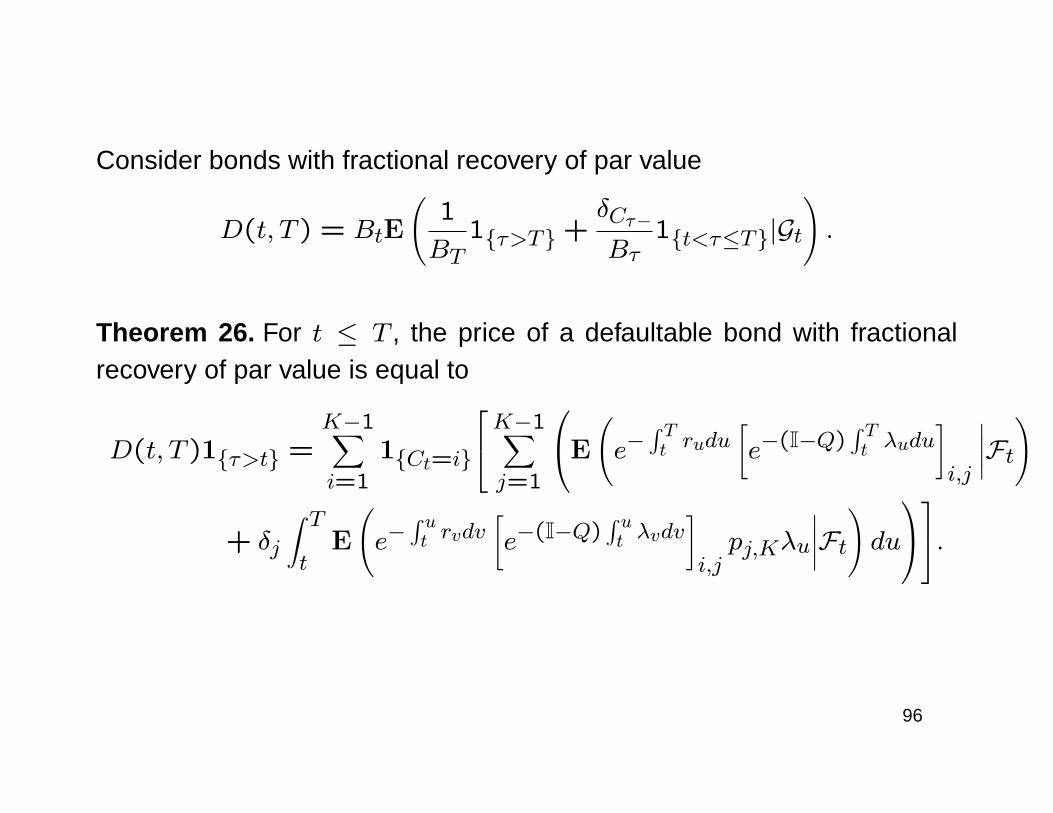
Consider bonds with fractional recovery of par value
D(t, T ) = BtE
(1
BT1τ>T +
δCτ−Bτ
1t<τ≤T|Gt).
Theorem 26. For t ≤ T , the price of a defaultable bond with fractionalrecovery of par value is equal to
D(t, T )1τ>t =K−1∑i=1
1Ct=i
K−1∑j=1
E
(e−∫ Tt rudu
[e−(I−Q)
∫ Tt λudu
]i,j
∣∣∣∣Ft)
+ δj
∫ Tt
E
(e−∫ ut rvdv
[e−(I−Q)
∫ ut λvdv
]i,jpj,Kλu
∣∣∣∣Ft)du
.
96

We are also interested in pricing credit derivatives connected with such de-faultable bond, for example in pricing of CDS on such bond. Credit DefaultSwap is an agreement between two parties protection seller and protectionbuyer. This contracts have two legs.
Premium Leg: Protection buyer agrees to pay fixed amount κ (CDS spread)at given dates T = T1 < T2 < . . . < Tn provided that default didn’thappened before or at Tn. For t ≤ T1 we have:
BtE
n∑k=1
κ
BTk1τ>Tk|Gt
.
Default Leg: Protection seller agrees to cover all losses on bond providedthat loss occurred before Tn, the protection horizon. For t ≤ T1 value ofthis leg is equal to
97
BtE
(1− δCτ−Bτ
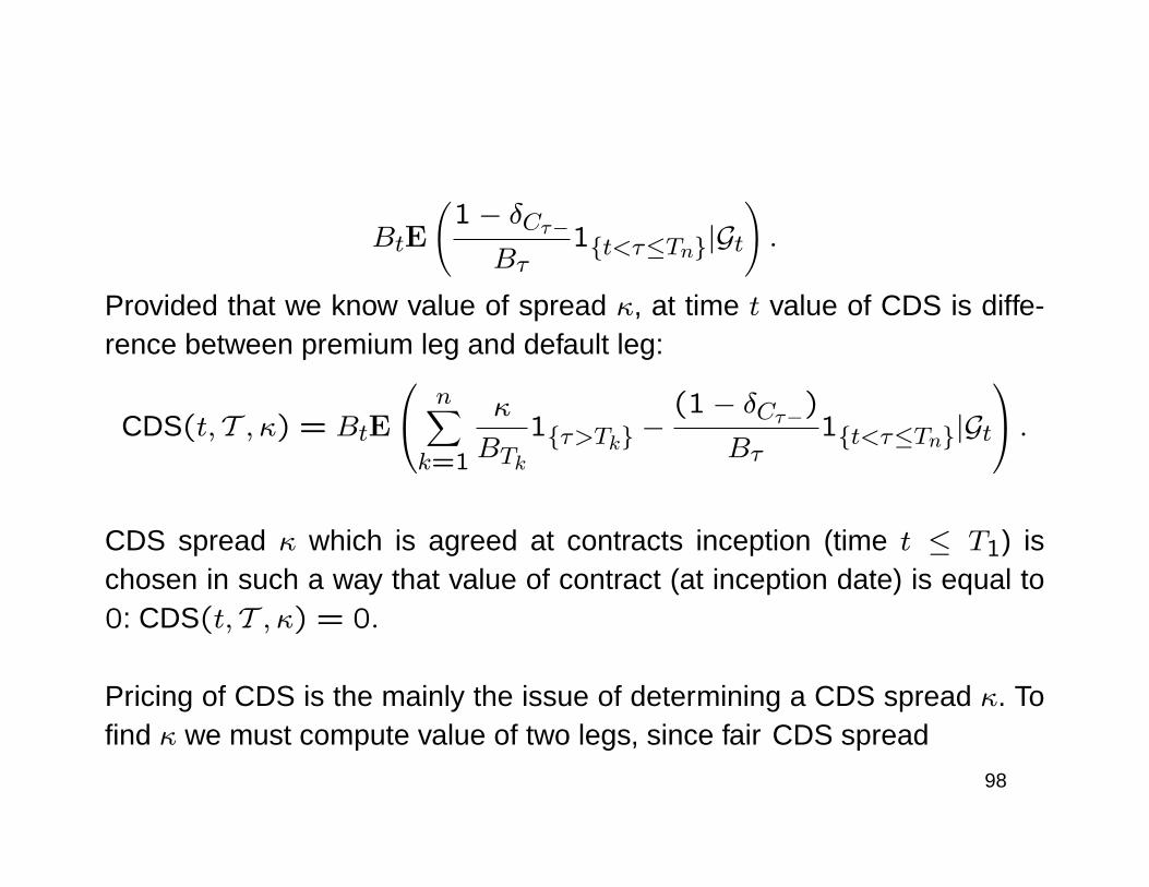
1t<τ≤Tn|Gt).
Provided that we know value of spread κ, at time t value of CDS is diffe-rence between premium leg and default leg:
CDS(t, T , κ) = BtE
n∑k=1
κ
BTk1τ>Tk −
(1− δCτ−)
Bτ1t<τ≤Tn|Gt
.CDS spread κ which is agreed at contracts inception (time t ≤ T1) ischosen in such a way that value of contract (at inception date) is equal to0: CDS(t, T , κ) = 0.
Pricing of CDS is the mainly the issue of determining a CDS spread κ. Tofind κ we must compute value of two legs, since fair CDS spread
98

is given as:
κ(t, T )1C(t) 6=K = 1C(t) 6=KE(BtBτ
(1− δCτ−)1t<τ≤Tn|Gt)
E(∑n
k=1BtBTk
1τ>Tk|Gt) .
Theorem 27. The value VD(t) of the default leg is equal to
K−1∑i=1
1Ct=i
K−1∑j=1
(1− δj)∫ Tnt
E
(e−∫ ut rvdv
[e−(I−Q)
∫ ut λvdv
]i,jpj,Kλu
∣∣∣∣Ft)du
.The value of the premium leg is given by
VP (t) =K−1∑i=1
1Ct=i
n∑k=1
K−1∑j=1
E
e− ∫ Tkt rudu
[e−(I−Q)
∫ Tkt λudu
]i,j
∣∣∣∣Ft .
99

References
T. Bielecki and M. Rutkowski,
joint works by T. Bielecki, S. Crepy, M. Jeanblanc and M. Rutkowski,
Th. Björk, G. DiMasi, Y. Kabanov and W. Runggaldier,
Th. Björk, Y. Kabanov and W. Runggaldier,
C. Blanchet-Scalliet and M. Jeanblanc.
D. Duffie and K. Singleton.
E. Eberlein and S. Raible; E. Eberlein and F. Özkan; E. Eberlein, J. Jacod and S. Raible,
D. Heath, R. Jarrow and A. Morton,
J. Jakubowski and J. Zabczyk; J.Jakubowski, M. Niewegłowski and J. Zabczyk,
J.Jakubowski and M. Niewegłowski,
R. A.Jarrow, D. Lando and S.Turnbull ,
D. Lando,
F. Özkan and T. Schmidt ,
T. Schmidt and W. Stute ,
P. J. Schönbucher .
100

Thank you for your attention.
101

![Unified Theory of Credit Spreads and Defaults · 2019-02-26 · OAS = E[Return Credit] + E[Other Factor] + Adjusted Aversion Coefficient * [Variance(Credit) + Variance(Other Factor)]](https://static.fdocument.org/doc/165x107/5e9267aa0c387321701b8ef5/unified-theory-of-credit-spreads-and-defaults-2019-02-26-oas-ereturn-credit.jpg)