Copyright © 2015, S. K. Mitra
13
1 Copyright © 2015, S. K. Mitra 1 • Recall that the transfer function of the first- order analog lowpass filter is given by • From above it follows that its differential equation representation is given by H LP (s) = Ω c s + Ω c Ω c > 0 dy(t ) dt + Ω c y(t ) = Ω c x(t ) , Copyright © 2015, S. K. Mitra 2 • Integrating the last equation we get whose block-diagram representation is y(t ) = Ω c [ x(τ ) − y(τ )]dτ −∞ t ∫ Copyright © 2015, S. K. Mitra 3 • Recall that the transfer function of the first- order analog highpass filter is given by • From above it follows that its differential equation representation is given by H HP (s) = s s + Ω c Ω c > 0 , dy(t ) dt + Ω c y(t ) = dx(t ) dt Copyright © 2015, S. K. Mitra • Integrating the last equation we get whose block-diagram representation is 4 y(t ) = x(t ) −Ω c y(τ )dτ −∞ t ∫ Copyright © 2015, S. K. Mitra • Recall that the transfer function of the first- order analog bandpass filter is given by • From above it follows that its differential equation representation is given by 5 d 2 y(t ) dt 2 + B dy(t ) dt + Ω o 2 y(t ) = B dx(t ) dt H BP (s) = Bs s 2 + Bs + Ω o 2 Ω o > 0 B > 0 , , Copyright © 2015, S. K. Mitra which can be rewritten as • Integrating the above equation twice we get 6 d 2 y(t ) dt 2 = B dx(t ) dt − dy(t ) dt −Ω o 2 y(t ) y(t ) = Bx(τ ) − y(τ ) ( ) −Ω o 2 y(ψ)dψ −∞ τ ∫ −∞ t ∫ dτ
Transcript of Copyright © 2015, S. K. Mitra
1
Copyright © 2015, S. K. Mitra 1
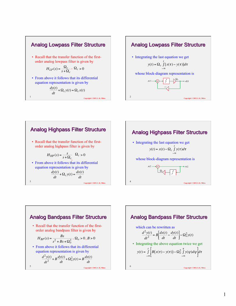
• Recall that the transfer function of the first-order analog lowpass filter is given by
• From above it follows that its differential equation representation is given by
€
HLP (s) = Ωcs +Ωc
Ωc > 0
€
dy(t)dt
+Ωcy(t) =Ωcx(t)
,
Copyright © 2015, S. K. Mitra 2
• Integrating the last equation we get
whose block-diagram representation is
€
y(t) =Ωc [x(τ )− y(τ )]dτ−∞
t∫
Copyright © 2015, S. K. Mitra 3
• Recall that the transfer function of the first-order analog highpass filter is given by
• From above it follows that its differential equation representation is given by
€
HHP (s) = ss +Ωc
Ωc > 0,
€
dy(t)dt
+Ωcy(t) =dx(t)dt
Copyright © 2015, S. K. Mitra
• Integrating the last equation we get
whose block-diagram representation is
4
€
y(t) = x(t)−Ωc y(τ )dτ−∞
t∫
Copyright © 2015, S. K. Mitra
• Recall that the transfer function of the first-order analog bandpass filter is given by
• From above it follows that its differential equation representation is given by
5
€
d2y(t)dt2
+ B dy(t)dt
+Ωo2y(t) = B dx(t)
dt€
HBP (s) =Bs
s2 + Bs +Ωo2 Ωo > 0 B > 0, ,
Copyright © 2015, S. K. Mitra
which can be rewritten as
• Integrating the above equation twice we get
6
€
d2y(t)dt2
= B dx(t)dt
−dy(t)dt
⎡ ⎣ ⎢
⎤ ⎦ ⎥ −Ωo
2y(t)
€
y(t) = B x(τ )− y(τ )( )−Ωo2 y(ψ)dψ−∞
τ∫
⎡
⎣ ⎢
⎤
⎦ ⎥
−∞
t∫ dτ
2
Copyright © 2015, S. K. Mitra
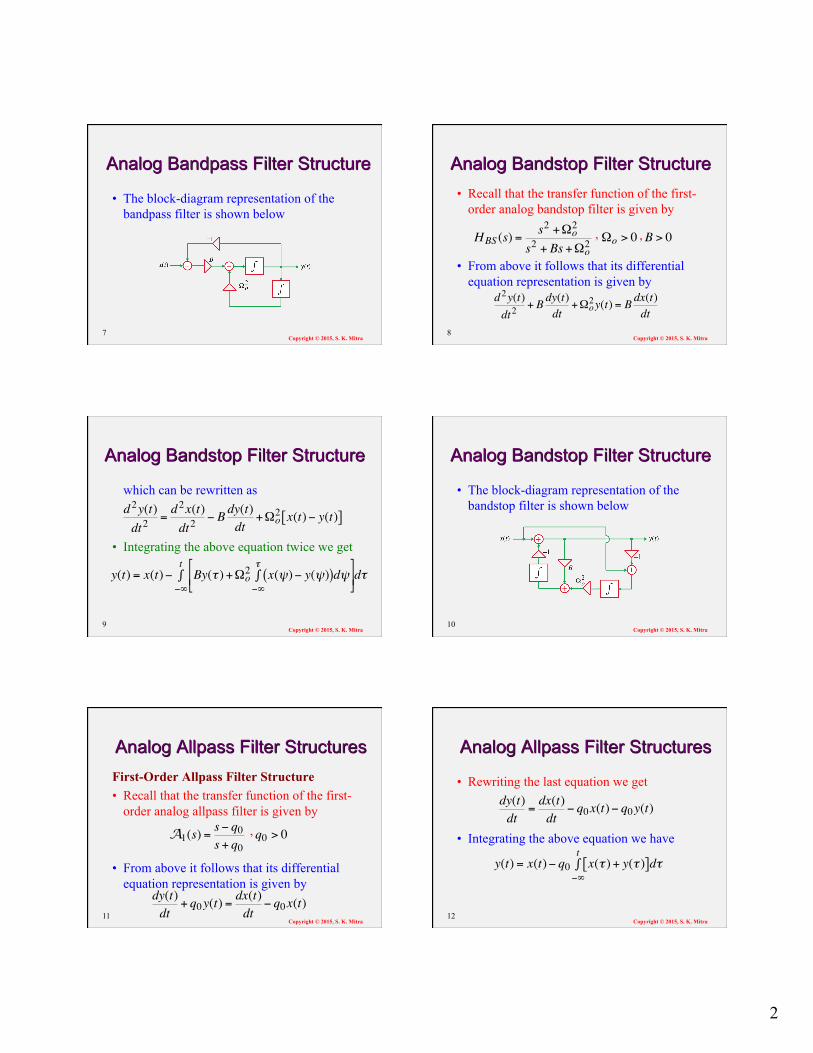
• The block-diagram representation of the bandpass filter is shown below
7 Copyright © 2015, S. K. Mitra
• Recall that the transfer function of the first-order analog bandstop filter is given by
• From above it follows that its differential equation representation is given by
8
€
HBS (s) =s2 +Ωo
2
s2 + Bs +Ωo2 Ωo > 0 B > 0
€
d2y(t)dt2
+ B dy(t)dt
+Ωo2y(t) = B dx(t)
dt
, ,
Copyright © 2015, S. K. Mitra
which can be rewritten as
• Integrating the above equation twice we get
9
€
d2y(t)dt2
=d2x(t)dt2
− B dy(t)dt
+Ωo2 x(t)− y(t)[ ]
€
y(t) = x(t)− By(τ )+Ωo2 x(ψ)− y(ψ)( )dψ−∞
τ∫
⎡
⎣ ⎢
⎤
⎦ ⎥
−∞
t∫ dτ
Copyright © 2015, S. K. Mitra
• The block-diagram representation of the bandstop filter is shown below
10
Copyright © 2015, S. K. Mitra
First-Order Allpass Filter Structure • Recall that the transfer function of the first-
order analog allpass filter is given by
• From above it follows that its differential equation representation is given by
11
€
A1(s) =s− q0s + q0
q0 > 0
€
dy(t)dt
+ q0y(t) =dx(t)dt
− q0x(t)
,
Copyright © 2015, S. K. Mitra
• Rewriting the last equation we get
• Integrating the above equation we have
12
€
dy(t)dt
=dx(t)dt
− q0x(t)− q0y(t)
€
y(t) = x(t)− q0 x(τ )+ y(τ )[ ]−∞
t∫ dτ
3
Copyright © 2015, S. K. Mitra
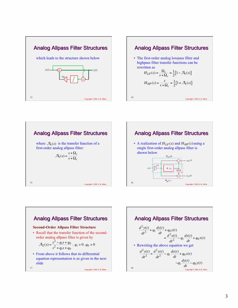
which leads to the structure shown below
13
x(t) y(t)+_q0
+
Copyright © 2015, S. K. Mitra
• The first-order analog lowpass filter and highpass filter transfer functions can be rewritten as
14
€
HLP (s) = Ωcs +Ωc
= 12 1−A1(s)[ ]
€
HHP (s) =s
s +Ωc= 12 1+A1(s)[ ]
Copyright © 2015, S. K. Mitra
where is the transfer function of a first-order analog allpass filter:
15
€
A1(s) =s +Ωcs +Ωc
€
A1(s)
Copyright © 2015, S. K. Mitra
• A realization of and using a single first-order analog allpass filter is shown below
16
€
HLP (s)
€
HHP (s)
Copyright © 2015, S. K. Mitra
Second-Order Allpass Filter Structure • Recall that the transfer function of the second-
order analog allpass filter is given by
• From above it follows that its differential equation representation is as given in the next slide
17
€
A2 (s) =s2 − q1s + q0s2 + q1s + q0
q1 > 0 q0 > 0, ,
Copyright © 2015, S. K. Mitra
• Rewriting the above equation we get
18
€
d2y(t)dt2
+ q1dy(t)dt
+ q0y(t)
€
=d2x(t)dt2
− q1dx(t)dt
+ q0x(t)
€
d2y(t)dt2
=d2x(t)dt2
− q1dx(t)dt
+ q0x(t)
€
−q1dy(t)dt
− q0y(t)
4
Copyright © 2015, S. K. Mitra
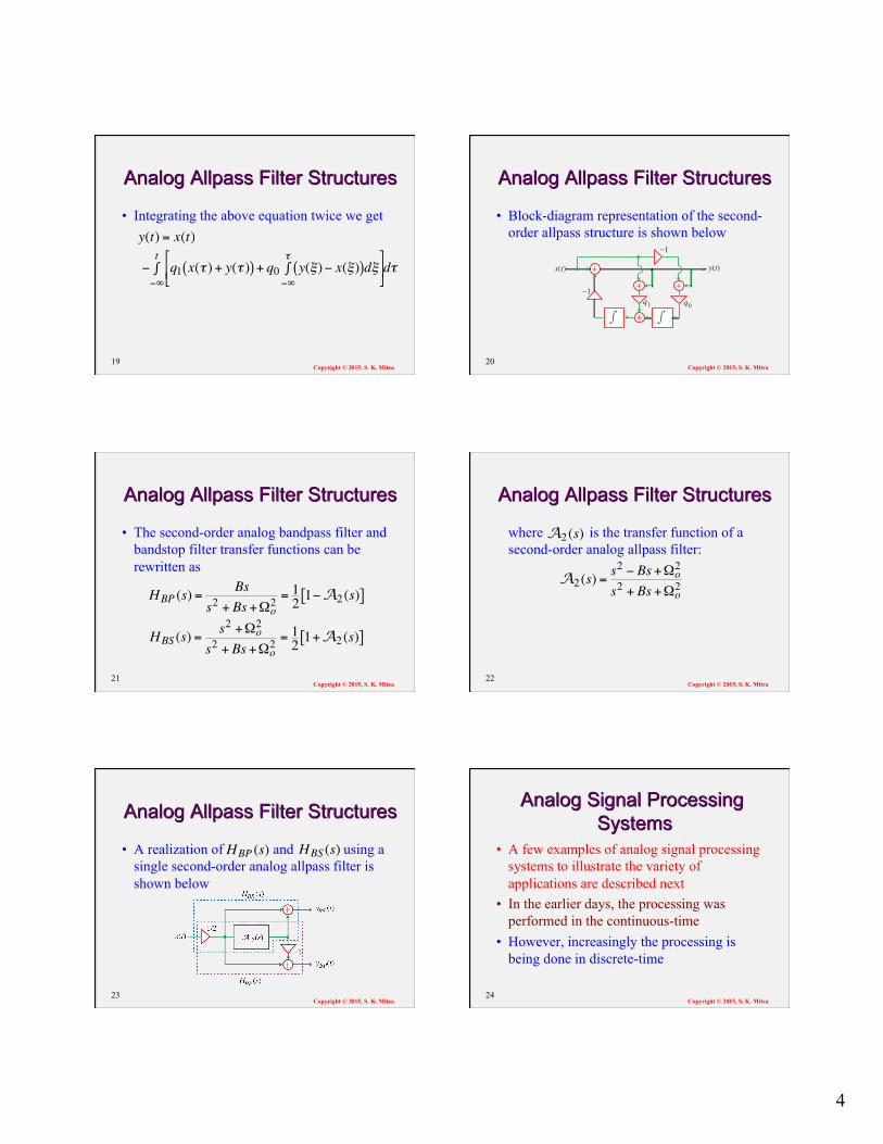
• Integrating the above equation twice we get
19
€
y(t) = x(t)
€
− q1 x(τ )+ y(τ )( ) + q0 y(ξ)− x(ξ)( )dξ−∞
τ∫
⎡
⎣ ⎢
⎤
⎦ ⎥
−∞
t∫ dτ
Copyright © 2015, S. K. Mitra
• Block-diagram representation of the second-order allpass structure is shown below
20
x(t) y(t)+
q0+
_1
_1
+ +q1
Copyright © 2015, S. K. Mitra
• The second-order analog bandpass filter and bandstop filter transfer functions can be rewritten as
21
€
HBP (s) =Bs
s2 + Bs +Ωo2 = 12 1−A2 (s)[ ]
€
HBS (s) =s2 +Ωo
2
s2 + Bs +Ωo2 = 12 1+A2 (s)[ ]
Copyright © 2015, S. K. Mitra
where is the transfer function of a second-order analog allpass filter:
22
€
A2 (s) =s2 − Bs +Ωo
2
s2 + Bs +Ωo2
€
A2 (s)
Copyright © 2015, S. K. Mitra
• A realization of and using a single second-order analog allpass filter is shown below
23
€
HBP (s)
€
HBS (s)
Copyright © 2015, S. K. Mitra
• A few examples of analog signal processing systems to illustrate the variety of applications are described next
• In the earlier days, the processing was performed in the continuous-time
• However, increasingly the processing is being done in discrete-time
24
5
Copyright © 2015, S. K. Mitra
• In many applications, the signal of interest gets corrupted by an unavoidable noise signal which is basically a random signal
• It is difficult to extract the desired information present in the original uncorrupted signal from the noise-corrupted signal
25 Copyright © 2015, S. K. Mitra
• Two very different ways a signal gets corrupted with noise (1) additive noise (2) multiplicative noise
• The model of the noise-corrupted signal in the additive noise case is given by
26
€
ψ(t) = x(t)+η(t)original signal noise
Copyright © 2015, S. K. Mitra
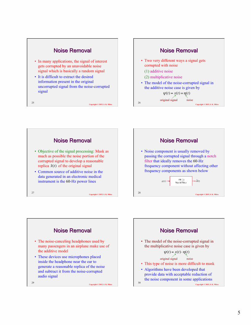
• Objective of the signal processing: Mask as much as possible the noise portion of the corrupted signal to develop a reasonable replica of the original signal
• Common source of additive noise in the data generated in an electronic medical instrument is the 60-Hz power lines
27
€
ˆ x (t)
Copyright © 2015, S. K. Mitra
• Noise component is usually removed by passing the corrupted signal through a notch filter that ideally removes the 60-Hz frequency component without affecting other frequency components as shown below
28
Copyright © 2015, S. K. Mitra
• The noise-canceling headphones used by many passengers in an airplane make use of the additive model
• These devices use microphones placed inside the headphone near the ear to generate a reasonable replica of the noise and subtract it from the noise-corrupted audio signal
29 Copyright © 2015, S. K. Mitra
• The model of the noise-corrupted signal in the multiplicative noise case is given by
• This type of noise is more difficult to mask • Algorithms have been developed that
provide data with acceptable reduction of the noise component in some applications
30
€
ψ(t) = x(t) ⋅η(t)original signal noise
6
Copyright © 2015, S. K. Mitra
• Various types of filters are used to modify the frequency response of a recording or the monitoring channel
• The shelving filter provides “boost” (rise) or “cut” (drop) in the gain response at either the low or the high end of the audio frequency range
31 Copyright © 2015, S. K. Mitra
• The peaking filters are used for midband equalization and are designed to have either a bandpass response to provide a boost or a bandstop response to provide a cut
32
Copyright © 2015, S. K. Mitra
• The transfer function of a first-order lowpass analog shelving filter for boost is given by
33 €
HLP(B)(s) =
s +KΩcs +Ωc
Ωc > 0 K >1, ,
Copyright © 2015, S. K. Mitra
• The transfer function of a first-order lowpass analog shelving filter for cut is given by
34 €
HLP(C)(s) =
s +Ωcs +Ωc /K
Ωc > 0 0 < K <1, ,
Copyright © 2015, S. K. Mitra
• The transfer function of a first-order highpass analog shelving filter for boost is given by
35 €
HHP(B)(s) =
Ks +Ωcs +Ωc
Ωc > 0 K >1, ,
Copyright © 2015, S. K. Mitra
• The transfer function of a first-order highpass analog shelving filter for cut is given by
36 €
HHP(C)(s) = K s +Ωc
s +KΩc
⎛
⎝ ⎜
⎞
⎠ ⎟ Ωc > 0 0 < K <1, ,
7
Copyright © 2015, S. K. Mitra
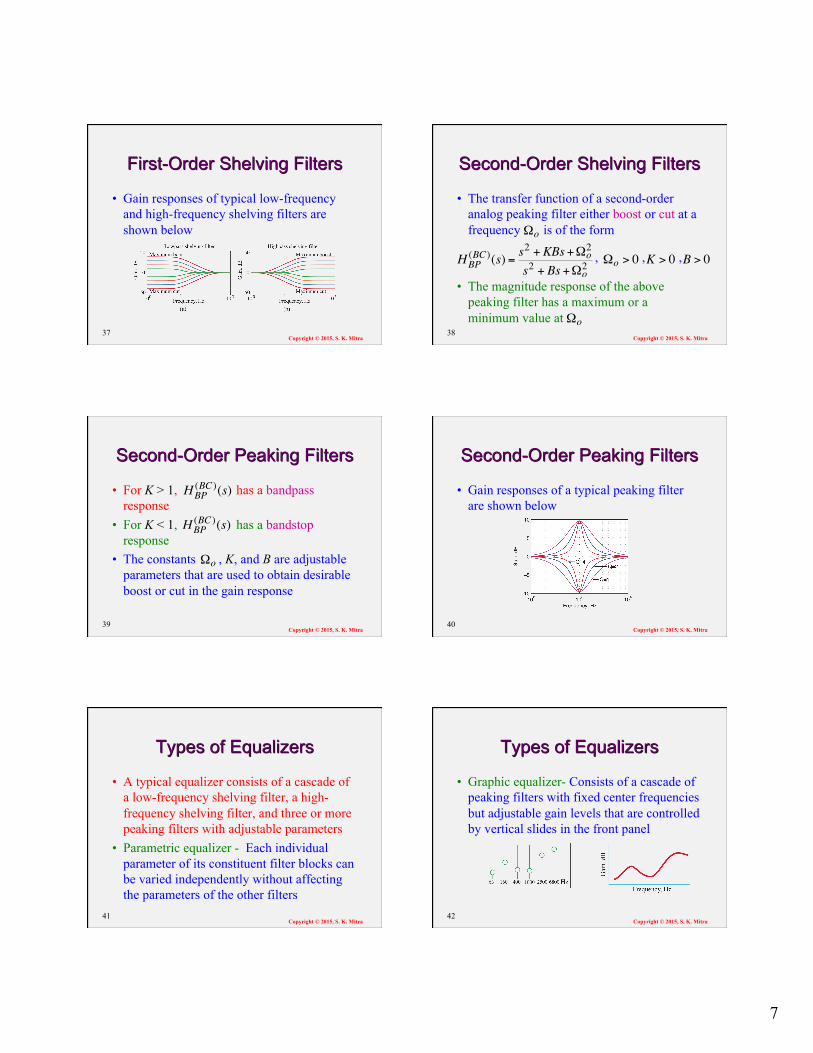
• Gain responses of typical low-frequency and high-frequency shelving filters are shown below
37 Copyright © 2015, S. K. Mitra
• The transfer function of a second-order analog peaking filter either boost or cut at a frequency is of the form
• The magnitude response of the above peaking filter has a maximum or a minimum value at
38
€
Ωo
€
HBP(BC)(s) =
s2 +KBs +Ωo2
s2 + Bs +Ωo2 Ωo > 0 K > 0 B > 0, , ,
€
Ωo
Copyright © 2015, S. K. Mitra
• For K > 1, has a bandpass response
• For K < 1, has a bandstop response
• The constants , K, and B are adjustable parameters that are used to obtain desirable boost or cut in the gain response
39
€
HBP(BC)(s)
€
Ωo
€
HBP(BC)(s)
Copyright © 2015, S. K. Mitra
• Gain responses of a typical peaking filter are shown below
40
Copyright © 2015, S. K. Mitra
• A typical equalizer consists of a cascade of a low-frequency shelving filter, a high-frequency shelving filter, and three or more peaking filters with adjustable parameters
• Parametric equalizer - Each individual parameter of its constituent filter blocks can be varied independently without affecting the parameters of the other filters
41 Copyright © 2015, S. K. Mitra
• Graphic equalizer- Consists of a cascade of peaking filters with fixed center frequencies but adjustable gain levels that are controlled by vertical slides in the front panel
42
8
Copyright © 2015, S. K. Mitra
• Analog filters that also find applications in the musical recording and transfer processes are the lowpass, highpass, and notch filters
• The notch filter is designed to attenuate a particular frequency component and has a narrow notch width so as not to affect the rest of the musical program
43 Copyright © 2015, S. K. Mitra
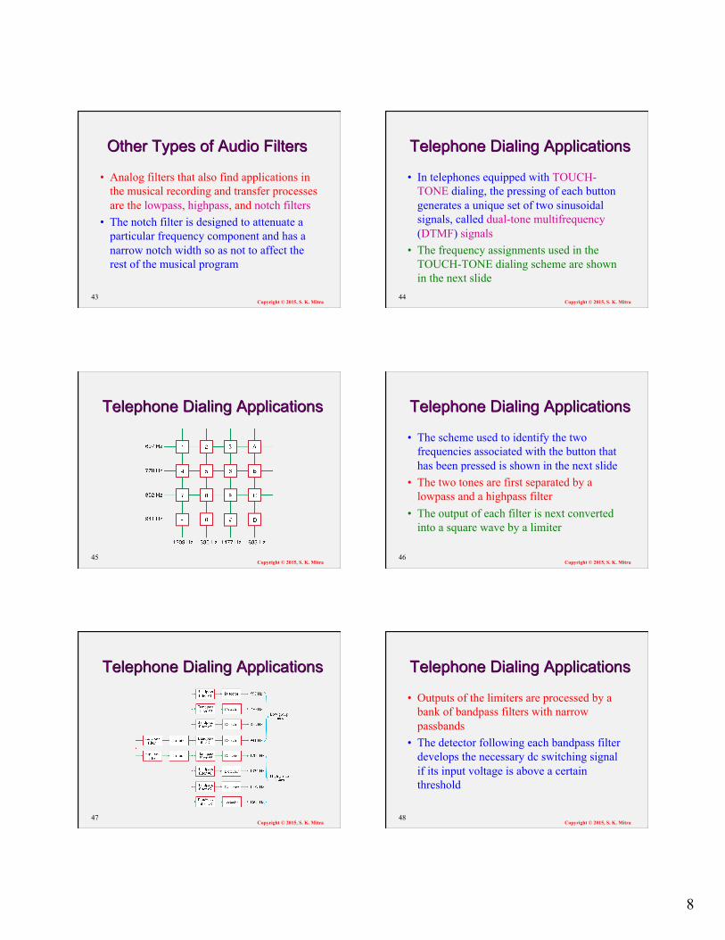
• In telephones equipped with TOUCH-TONE dialing, the pressing of each button generates a unique set of two sinusoidal signals, called dual-tone multifrequency (DTMF) signals
• The frequency assignments used in the TOUCH-TONE dialing scheme are shown in the next slide
44
Copyright © 2015, S. K. Mitra 45
Copyright © 2015, S. K. Mitra
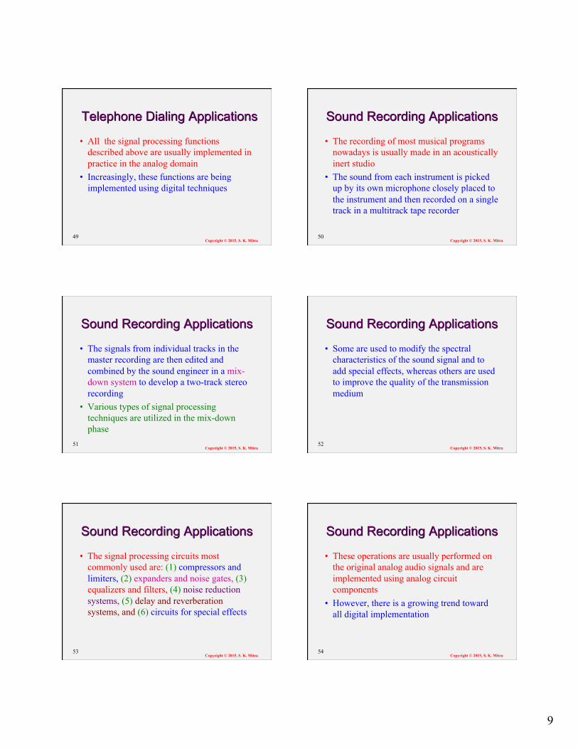
• The scheme used to identify the two frequencies associated with the button that has been pressed is shown in the next slide
• The two tones are first separated by a lowpass and a highpass filter
• The output of each filter is next converted into a square wave by a limiter
46
Copyright © 2015, S. K. Mitra 47
Copyright © 2015, S. K. Mitra
• Outputs of the limiters are processed by a bank of bandpass filters with narrow passbands
• The detector following each bandpass filter develops the necessary dc switching signal if its input voltage is above a certain threshold
48
9
Copyright © 2015, S. K. Mitra
• All the signal processing functions described above are usually implemented in practice in the analog domain
• Increasingly, these functions are being implemented using digital techniques
49 Copyright © 2015, S. K. Mitra
• The recording of most musical programs nowadays is usually made in an acoustically inert studio
• The sound from each instrument is picked up by its own microphone closely placed to the instrument and then recorded on a single track in a multitrack tape recorder
50
Copyright © 2015, S. K. Mitra
• The signals from individual tracks in the master recording are then edited and combined by the sound engineer in a mix-down system to develop a two-track stereo recording
• Various types of signal processing techniques are utilized in the mix-down phase
51 Copyright © 2015, S. K. Mitra
• Some are used to modify the spectral characteristics of the sound signal and to add special effects, whereas others are used to improve the quality of the transmission medium
52
Copyright © 2015, S. K. Mitra
• The signal processing circuits most commonly used are: (1) compressors and limiters, (2) expanders and noise gates, (3) equalizers and filters, (4) noise reduction systems, (5) delay and reverberation systems, and (6) circuits for special effects
53 Copyright © 2015, S. K. Mitra
• These operations are usually performed on the original analog audio signals and are implemented using analog circuit components
• However, there is a growing trend toward all digital implementation
54
10
Copyright © 2015, S. K. Mitra
• The compressor can be considered as an amplifier with two gain levels
• For a downward compressor, the gain is unity for input signal levels below a certain threshold and less than unity for signals with levels above the threshold
55 Copyright © 2015, S. K. Mitra
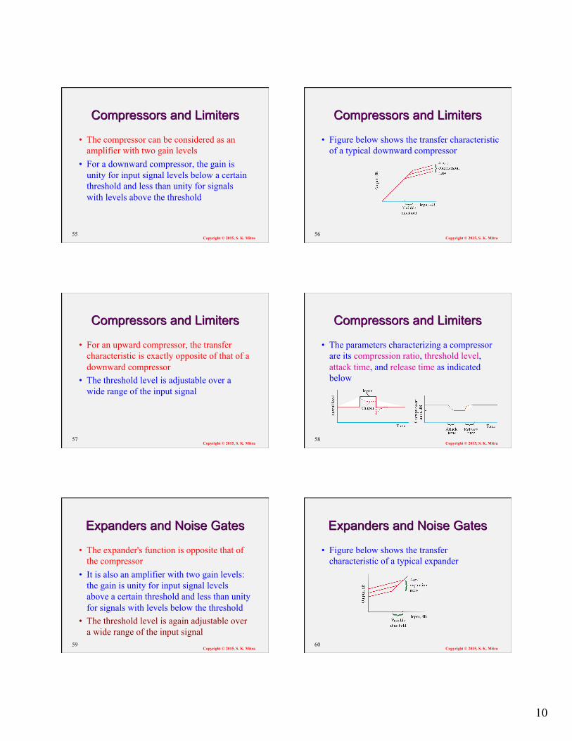
• Figure below shows the transfer characteristic of a typical downward compressor
56
Copyright © 2015, S. K. Mitra
• For an upward compressor, the transfer characteristic is exactly opposite of that of a downward compressor
• The threshold level is adjustable over a wide range of the input signal
57 Copyright © 2015, S. K. Mitra
• The parameters characterizing a compressor are its compression ratio, threshold level, attack time, and release time as indicated below
58
Copyright © 2015, S. K. Mitra
• The expander's function is opposite that of the compressor
• It is also an amplifier with two gain levels: the gain is unity for input signal levels above a certain threshold and less than unity for signals with levels below the threshold
• The threshold level is again adjustable over a wide range of the input signal
59 Copyright © 2015, S. K. Mitra
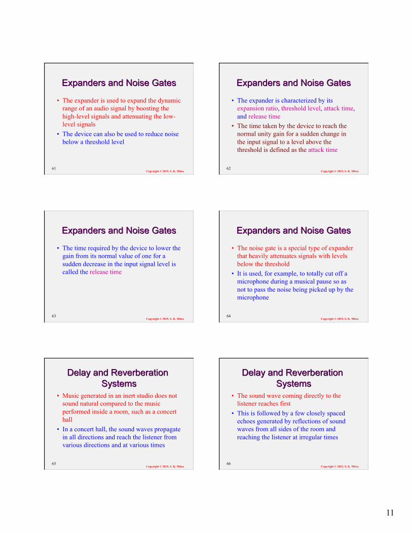
• Figure below shows the transfer characteristic of a typical expander
60
11
Copyright © 2015, S. K. Mitra
• The expander is used to expand the dynamic range of an audio signal by boosting the high-level signals and attenuating the low-level signals
• The device can also be used to reduce noise below a threshold level
61 Copyright © 2015, S. K. Mitra
• The expander is characterized by its expansion ratio, threshold level, attack time, and release time
• The time taken by the device to reach the normal unity gain for a sudden change in the input signal to a level above the threshold is defined as the attack time
62
Copyright © 2015, S. K. Mitra
• The time required by the device to lower the gain from its normal value of one for a sudden decrease in the input signal level is called the release time
63 Copyright © 2015, S. K. Mitra
• The noise gate is a special type of expander that heavily attenuates signals with levels below the threshold
• It is used, for example, to totally cut off a microphone during a musical pause so as not to pass the noise being picked up by the microphone
64
Copyright © 2015, S. K. Mitra
• Music generated in an inert studio does not sound natural compared to the music performed inside a room, such as a concert hall
• In a concert hall, the sound waves propagate in all directions and reach the listener from various directions and at various times
65 Copyright © 2015, S. K. Mitra
• The sound wave coming directly to the listener reaches first
• This is followed by a few closely spaced echoes generated by reflections of sound waves from all sides of the room and reaching the listener at irregular times
66
12
Copyright © 2015, S. K. Mitra
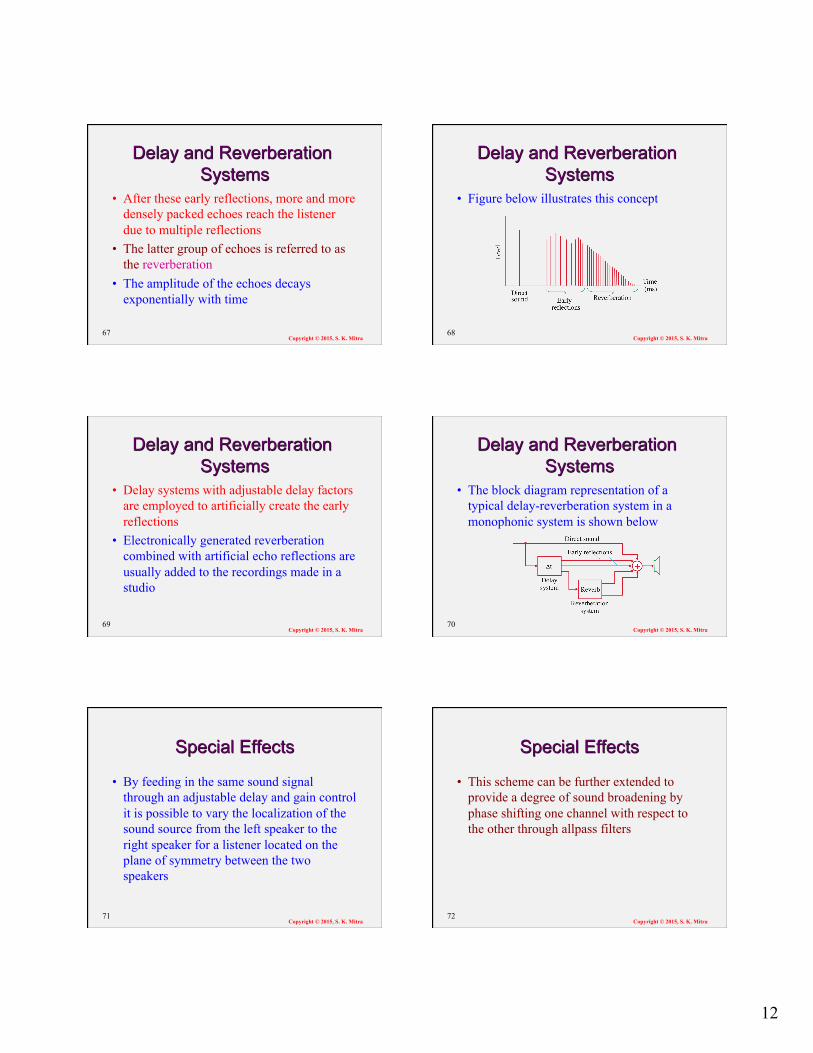
• After these early reflections, more and more densely packed echoes reach the listener due to multiple reflections
• The latter group of echoes is referred to as the reverberation
• The amplitude of the echoes decays exponentially with time
67 Copyright © 2015, S. K. Mitra
• Figure below illustrates this concept
68
Copyright © 2015, S. K. Mitra
• Delay systems with adjustable delay factors are employed to artificially create the early reflections
• Electronically generated reverberation combined with artificial echo reflections are usually added to the recordings made in a studio
69 Copyright © 2015, S. K. Mitra
• The block diagram representation of a typical delay-reverberation system in a monophonic system is shown below
70
Copyright © 2015, S. K. Mitra
• By feeding in the same sound signal through an adjustable delay and gain control it is possible to vary the localization of the sound source from the left speaker to the right speaker for a listener located on the plane of symmetry between the two speakers
71 Copyright © 2015, S. K. Mitra
• This scheme can be further extended to provide a degree of sound broadening by phase shifting one channel with respect to the other through allpass filters
72
13
Copyright © 2015, S. K. Mitra
• Another application of the delay-reverberation system is in the processing of a single track into a pseudo-stereo format while simulating a natural acoustical environment
• The delay system can also be used to generate a chorus effect from the sound of a soloist
73