COMPLEXNUMBERSANDGEOMETRY - JKUset). This means that the computations required will be particularly...
27
COMPLEX NUMBERS AND GEOMETRY by J.B. Cooper
Transcript of COMPLEXNUMBERSANDGEOMETRY - JKUset). This means that the computations required will be particularly...
COMPLEX NUMBERS AND GEOMETRY
byJ.B. Cooper
Inhaltsverzeichnis
1 Geometry and function theory 11.1 Normal families . . . . . . . . . . . . . . . . . . . . . . . . . . . . . . . . . . . . . . . 11.2 Domains as Riemann manifolds . . . . . . . . . . . . . . . . . . . . . . . . . . . . . . 31.3 Curvature . . . . . . . . . . . . . . . . . . . . . . . . . . . . . . . . . . . . . . . . . . 71.4 Appendix . . . . . . . . . . . . . . . . . . . . . . . . . . . . . . . . . . . . . . . . . . 12
i
1 GEOMETRY AND FUNCTION THEORY 1
1 Geometry and function theory
1.1 Normal families
We consider now the space H(U) of holomorphicic functions on a domain U . We regard this as aFrechet space (complete metrisable locally convex space) with the countable family pn of seminormswhere pn(f) is the supremum of the absolute value of f on Kn and (Kn) is a (countable) basis for thecompact subsets of U . We shall only require the following facts about the corresponding topology—it is metrisable and convergence means uniform convergence on compact subsets of U i.e. almostuniform convergence. (see Appendix).Then we have the following characterisation of the relatively compact subsets of H(U) which followsfrom the theorem of Ascoli and the Cauchy integral theorem:
Proposition 1.1 A subset A of C(U) is relatively compact if and only if it is uniformly boundedon compacta and equicontinuous on compacta. A ⊂ H(U) is relatively compact if and only if it isuniformly bounded on compacta.
Proof. The first statement is simply a special case of the version of Ascoli’s theorem formulated inthe Appendix (to Chapter 2). In order to prove the second case we begin by assuming that U is theunit disc D. We shall then show below how to deduce the general case from this one by a generallocalisation principle.By Ascoli’s theorem and the Weierstraß result on the almost uniform limit of analytic functions, itsuffices to show that a family A which is bounded on compacta is equicontinuous on compacta. Forthis it suffices to show that if is equicontinuous on each set of the type
Dr = z : |z| ≤ r
for 0 < r < 1. In fact it is uniformly Lipschitz since its the derivatives are uniformly bounded on thisset (see Appendix). This follows from the Cauchy estimates
|f ′(z)| ≤MR (|z| ≤ r)
where R is chosen between r and 1 and MR = sup|f(z)| : |z| ≤ R, f ∈ A.
In particular we have Montel’s theorem—if A is uniformly bounded, then it is relatively compact i.e.each sequence in A has a subsequence which converges almost uniformly to an analytic function.Relatively compact subsets of H(U) are traditionally called normal families.We remark here that the classical definition of normality, in fact, runs as follows: A set A is normalif and only if each sequence in A has a subsequence as above, or one that converges at each point toinfinity. Thus for example, the sequence nz : n ∈ N is normal in H(G) where G = C \ 0 but notin H(C). We shall consider this type of normality later in what we regard as its natural setting, thatof meromorphic functions. The reader can verify (this requires the use of Hurwitz’ theorem) that thefamily A is normal in this sense if and only if it is relatively compact as a subset of the space ofcontinuous functions from U into the extended complex plane.We now indicate in a sequence of lemmata how to deduce the general version of the above resultfrom the case of functions on the disc.
Lemma 1.2 A subset F ⊂ H(U) is normal if and only if it is normal at each point i.e. for each zthere is a neighbourhood of z on which the restrictions of the functions of F are normal).
1 GEOMETRY AND FUNCTION THEORY 2
Proof. We sketch the proof which is a typical application of the diagonal method. It is trivial thatnormality on any domain implies the same property on each subdomain. Hence it suffices to showthat local normality implies normality. For each z ∈ U there is a rz so that F is normal on thedisc with centre z and radius rz. The open balls U(z, rz) cover U and so by the Lindelof property ofseparable metric spaces (see Appendix) we can cover U by a sequence of such balls—we denote thissequence by (Un). We now proceed by menas of the diagonal procedure (see Appendix). Namely wechoose successively subsequences (fk
n) where
a) the sequence (fk+1n )n is a subsequence of (f
kn)n. (By convention, we identify the original sequence
with (f 0n)n).
b) the sequence (fkn)n converges uniformly onf Uk. Then the diagonal sequence (fk
k )k can be seento converge almost uniformly.
In a similar way one can show that if F is a subset of H(U), then the following conditions areequivalent.
1. F is bounded on compacta i.e. for each K compact in U F is uniformly bounded on K;
2. F is locally bounded i.e. each z ∈ U has a neighbourhood on which F is uniformly bounded.
Now using the Cauchy estimates it is easy to show that if F satisfies the second condition, then thecorresponding family F ′ = ′ : | ∈ F of derivatives also satisfies it. Hence we have the result
Proposition 1.3 If F is a subset of H(U) which is uniformly bounded on compacta then so isf ′ : f ∈ F.We remark that from the above it follows that if A is a locally bounded subset of H(U) then it isequicontinuous (since the derivates are locally bounded and this implies that the restrictions of A tocompact subsets are uniformly Lipshitz continuous).We close with a famous result of classical function theory which can easily proved using these ideas.
Exercise 1.4 Prove the theorem of Vitali-Porter: Let (fn) be a locally bounded sequence in H(U),f ∈ H(U) so that lim fn(z) exists for each z in a subset A of U which has an accumulation point inU . Show that there is then an f ∈ H(U) so that fn → f almost uniformly. (Compare the (compact)topology of almost uniform convergence with the Hausdorff topology of pointwise convergence on A).
One of the main applications of normal families is to the proof of the Riemann mapping theorem:
Proposition 1.5 Let the domain U be a proper subset of C and simply connected (equivalently,homeomorphic to D). Then U is conformally equivalent to D.
Proof. We begin the proof with the following two reductions.Firstly we note that if the closure of U is a proper subset of C (i.e. U is not dense in C), then we canfind a disc in the exterior of U . Inversion in this disc is a conformal mapping of U onto a boundedset.On the other hand since U is simply connected, we can define a branch of the logarithm on U . (Forconvenience, we assume that 0 /∈ U and 1 ∈ U—we can clearly arrange this by simple transformations.Then we define
ln z =
∫
γ
1
zdz
1 GEOMETRY AND FUNCTION THEORY 3
where γ is a path from 1 to z in U . By the condition of simply connectedness, this is independent ofthe path and so is an analytic function). By the usual argument the image of U ander this function(which is then conformally equivalent to U) satisfies the conditions of the previous paragraph.Hence combining these two arguments we can reduce to the case where U is a bounded region.We now introduce for a fixed P in U the family
F = : U → D : is 1− 1, holomorphicic and (P) = ′.
This is non-empty (since we can find such a function on any bounded disc). By Montel’s theorem,F is normal.
Now we set M = sup|f ′(P )| : f ∈ F and find a sequence (fn) with |fn′(P )| ≥M − 1
n.
Since F is normal we can, by going over to a subsequence, assume that fn converges in H(U), sayto f . We claim that f ∈ F and (as is obvious) |f ′(P )| = M i.e. the above supremum is attained.Firstly we note that f is non-constant (why?). Secondly, f takes its values in D as the limit of thefn. But it then follows from the maximum modulus theorem that in fact its image is a subset of D.It can easily be deduced using Hurwitz’ theorem that f is also 1− 1 (Exercise).Hence it remains to show that f is onto. This is where the concrete analysis comes in. We shallshow that if f is not onto, then we can find a g in F with too large a value for |g′(P )|. Assumetherefore that f is not onto. Suppose that the value β is owithted. We now compose with the Mobiustransformation φβ to get a function F which owis the value 0. Since this function is defined on asimply connected domain, we can again as above define a function lnF (by putting
lnF (z) =
∫
F ′(ζ)
F (ζdζ,
the integral being taken along any path in U from P to z). We can then define F α for any α byputting
F α(z) = exp(α lnF (z)).
Putting this together we define an analytic function µ where
µ(z) = (φβ f(z))1/2 .
Then we put
ν(z) =|µ′(P )|µ′(P )
φτ µ(z)
where τ = µ(P ). Then ν ∈ F and one can compute that
ν ′(P )| = 1 + |β|2|β|1/2M
and this is strictly greater then M . This contradiction proves the result.
1.2 Domains as Riemann manifolds
We shall now apply some of the results of the previous chapter to obtain two of the most remarkableresults on analytic functions, the theorems of Picard. In order to do this we shall consider opensubsets of C = R2 as local Riemannian manifolds of a particularly simple type, namely where themetric tensor is a multiple of the ordinary scalar product (the factor depending on the point in theset). This means that the computations required will be particularly simple.
1 GEOMETRY AND FUNCTION THEORY 4
If z ∈ Ω and ξ is in C = R2, we define
‖ξ‖ρ,z = ρ(z)|ξ|.
Then the length ℓρ(γ) of a path is gigen by the equation
ℓρ(γ) =
∫ b
a
‖γ′(s)‖ρ,γ(s) ds.
([a, b] is the parametrising interval). Note that we are not implying by the use of the symbols γ ands that γ has arc length parametrisation (as we did in chapter 2).In the following we shall often use the notation P , Q etc. to denote points of the local manifold Uwhen we are emphasising the geometric interpretation. Of course they are also points of the complexplane and so can be denoted by z, w etc. We shall sometimes even write zP to denote the complexnumber corresponding to the geometrical point P on the manifold. If P and Q are points in U , thenthe geodetic distance is
ρ(P,Q) = infℓρ(γ)the infimum being taken over all paths in U from P to Q.We remark that it follows from a general theorem on Riemann manifolds that the above infimum isattained (i.e. there is a path from P to Q with length ρ(P,Q)) for each pair P , Q if and only if U iscomplete under the metric ρ (it is relatively easy to see that the latter is a metric).In the language of the previous chapter we are dealing with the local Riemann manifold U withmetric tensor (first fundamental form)
G =
[
ρ2(x, y) 00 ρ2(x, y)
]
(i.e. “ds2 = ρ2(dx2 + dy2)”).Then g =
√detG = ρ2 and
G−1 =
[
1/ρ2 00 1/ρ2
]
.
Our main examples will be
Ω = D and ρ =1
1− |z|2resp.
Ω = H+ = z ∈ C : ℑz > 0 with ρ =1
y2.
In fact these spaces are essentially the same and are models for non-euclidean (hyperbolic) geometry.
Example 1.6 A routine calculation show that the length of the curve γ(t) = t (0 ≤ t ≤ 1− ǫ) in the
Poincare metric1
1− |z|2 is 12ln
2− ǫ
ǫ. For the length is
∫ 1−ǫ
0
1
1− t2dt
which gives the above expression. If we put R = 1− ǫ then it takes the form
1
2ln
1 +R
1− R.
This result can be reinterpreted as the fact that if P = 0 and Q = (R, 0) where 0 < R < 1, thenρ(P,Q) = 1
2ln(
1+R1−R
)
. (It is intuitively obvious and easy to demonstrate that the above path is the
1 GEOMETRY AND FUNCTION THEORY 5
shortest route from P and Q. In fact if we consider a curve of the form γ(t) = t+ ib(t) with b(0) = 0,b(1− ǫ) = 1− ǫ, then it length is
∫ 1−ǫ
0
(1 + b′(t)2)1/2
1− t2 − b(t)2dt
which is clearly larger than the above value).
We remark that the metrics on D and H+ above define the usually topology on these subsets ofC. However, they are not metrically equivalent to the euclidean metrics there. In fact both of thesemetrics are complete (see below)
Definition 1.7 Suppose now that f : Ω1 → Ω2 is a non-constant holomorphic function. If ρ is ametric on Ω2, we define the induced metric f ∗ρ on Ω1 by putting
f ∗ρ(z) = ρ(f(z))
∣
∣
∣
∣
∂f
∂z
∣
∣
∣
∣
.
If f is a bijection and ρ1 resp. ρ2 are metrics on the above spaces, then f is an isometry if f ∗ρ2 = ρ1.Then f−1 is also an isometry.A simple calculation shows that then ℓρ1(γ) = ℓρ2(f γ) for each curve in Ω1 and so that ρ1(P,Q) =ρ2(f(P ), f(Q)) for P ,Q in Ω1.
For example one can show that if h is a conformal mapping of D, then h is an isometry for thePoincare metric. For this it suffices to consider the two cases ρτ and φa discussed above:
Case 1. w = eiτz. Then h′(z) = eiτ and so its absolute value is 1. Hence
h∗ρ(z) = ρ(w) =1
1− |w|2 =1
1− |z|2 = ρ(z).
Case 2. w =z − a
1− az. Then
h∗ρ(z) = ρ(w)
∣
∣
∣
∣
dw
dz
∣
∣
∣
∣
=1
1− |a−a|2|1−az|2
1− |a|2|1− az|2
=1− |a|2
|1− az|2 − |z − a|2
=1− |a|2
(1− |a|2)(1− |z|2) .
From this we can deduce the following formula:
Proposition 1.8 If P and Q are points of D, then
ρ(P,Q) =1
2ln
1 +∣
∣
∣
P−Q1−PQ
∣
∣
∣
1−∣
∣
∣
P−Q1−PQ
∣
∣
∣
.
1 GEOMETRY AND FUNCTION THEORY 6
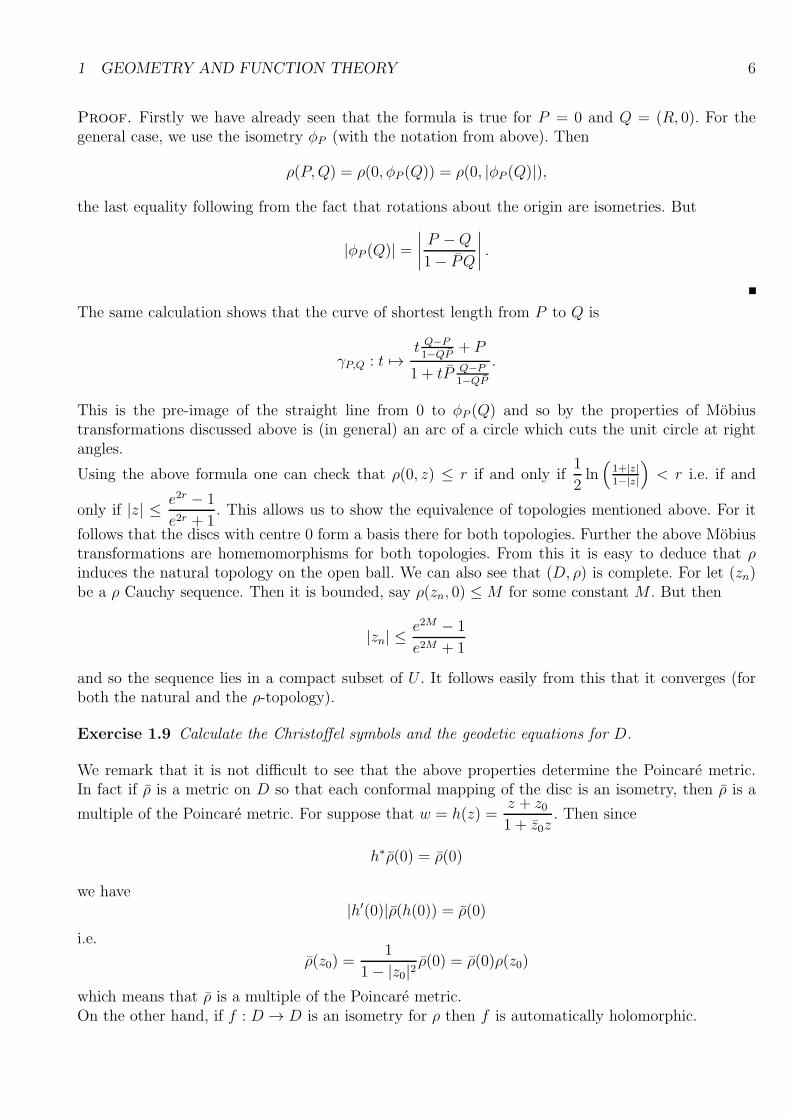
Proof. Firstly we have already seen that the formula is true for P = 0 and Q = (R, 0). For thegeneral case, we use the isometry φP (with the notation from above). Then
ρ(P,Q) = ρ(0, φP (Q)) = ρ(0, |φP (Q)|),
the last equality following from the fact that rotations about the origin are isometries. But
|φP (Q)| =∣
∣
∣
∣
P −Q
1− PQ
∣
∣
∣
∣
.
The same calculation shows that the curve of shortest length from P to Q is
γP,Q : t 7→t Q−P1−QP
+ P
1 + tP Q−P1−QP
.
This is the pre-image of the straight line from 0 to φP (Q) and so by the properties of Mobiustransformations discussed above is (in general) an arc of a circle which cuts the unit circle at rightangles.
Using the above formula one can check that ρ(0, z) ≤ r if and only if1
2ln(
1+|z|1−|z|
)
< r i.e. if and
only if |z| ≤ e2r − 1
e2r + 1. This allows us to show the equivalence of topologies mentioned above. For it
follows that the discs with centre 0 form a basis there for both topologies. Further the above Mobiustransformations are homemomorphisms for both topologies. From this it is easy to deduce that ρinduces the natural topology on the open ball. We can also see that (D, ρ) is complete. For let (zn)be a ρ Cauchy sequence. Then it is bounded, say ρ(zn, 0) ≤M for some constant M . But then
|zn| ≤e2M − 1
e2M + 1
and so the sequence lies in a compact subset of U . It follows easily from this that it converges (forboth the natural and the ρ-topology).
Exercise 1.9 Calculate the Christoffel symbols and the geodetic equations for D.
We remark that it is not difficult to see that the above properties determine the Poincare metric.In fact if ρ is a metric on D so that each conformal mapping of the disc is an isometry, then ρ is a
multiple of the Poincare metric. For suppose that w = h(z) =z + z01 + z0z
. Then since
h∗ρ(0) = ρ(0)
we have|h′(0)|ρ(h(0)) = ρ(0)
i.e.
ρ(z0) =1
1− |z0|2ρ(0) = ρ(0)ρ(z0)
which means that ρ is a multiple of the Poincare metric.On the other hand, if f : D → D is an isometry for ρ then f is automatically holomorphic.
1 GEOMETRY AND FUNCTION THEORY 7
Proof. For by the usual reduction we can assume that f(0) = 0. Then as above the circle CR =z : |z| = R is mapped onto itself for each 0 < R < 1. This means that for any P
|f(P )− f(0)||P − 0| =
|f(P )||P |
and so f is conformal at 0 (in the sense that it preserves angles between curves). Once again bythe homogeneity, this holds everywhere. But by the result sketched in the second chapter on thegeometrical charaterisation of conformal mappings, this implies that f is either holomorphic or anti-
holomorphic. The latter case is impossible (since then
∣
∣
∣
∣
∂f
∂z
∣
∣
∣
∣
= 0).
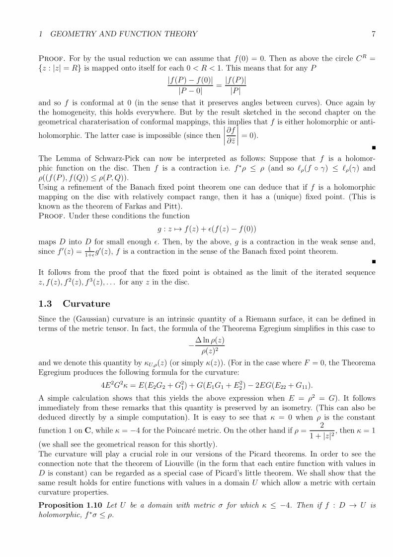
The Lemma of Schwarz-Pick can now be interpreted as follows: Suppose that f is a holomor-phic function on the disc. Then f is a contraction i.e. f ∗ρ ≤ ρ (and so ℓρ(f γ) ≤ ℓρ(γ) andρ((f(P ), f(Q)) ≤ ρ(P,Q)).Using a refinement of the Banach fixed point theorem one can deduce that if f is a holomorphicmapping on the disc with relatively compact range, then it has a (unique) fixed point. (This isknown as the theorem of Farkas and Pitt).Proof. Under these conditions the function
g : z 7→ f(z) + ǫ(f(z)− f(0))
maps D into D for small enough ǫ. Then, by the above, g is a contraction in the weak sense and,since f ′(z) = 1
1+ǫg′(z), f is a contraction in the sense of the Banach fixed point theorem.
It follows from the proof that the fixed point is obtained as the limit of the iterated sequencez, f(z), f 2(z), f 3(z), . . . for any z in the disc.
1.3 Curvature
Since the (Gaussian) curvature is an intrinsic quantity of a Riemann surface, it can be defined interms of the metric tensor. In fact, the formula of the Theorema Egregium simplifies in this case to
−∆ ln ρ(z)
ρ(z)2
and we denote this quantity by κU,ρ(z) (or simply κ(z)). (For in the case where F = 0, the TheoremaEgregium produces the following formula for the curvature:
4E2G2κ = E(E2G2 +G21) +G(E1G1 + E2
2)− 2EG(E22 +G11).
A simple calculation shows that this yields the above expression when E = ρ2 = G). It followsimmediately from these remarks that this quantity is preserved by an isometry. (This can also bededuced directly by a simple computation). It is easy to see that κ = 0 when ρ is the constant
function 1 on C, while κ = −4 for the Poincare metric. On the other hand if ρ =2
1 + |z|2 , then κ = 1
(we shall see the geometrical reason for this shortly).The curvature will play a crucial role in our versions of the Picard theorems. In order to see theconnection note that the theorem of Liouville (in the form that each entire function with values inD is constant) can be regarded as a special case of Picard’s little theorem. We shall show that thesame result holds for entire functions with values in a domain U which allow a metric with certaincurvature properties.
Proposition 1.10 Let U be a domain with metric σ for which κ ≤ −4. Then if f : D → U isholomorphic, f ∗σ ≤ ρ.
1 GEOMETRY AND FUNCTION THEORY 8
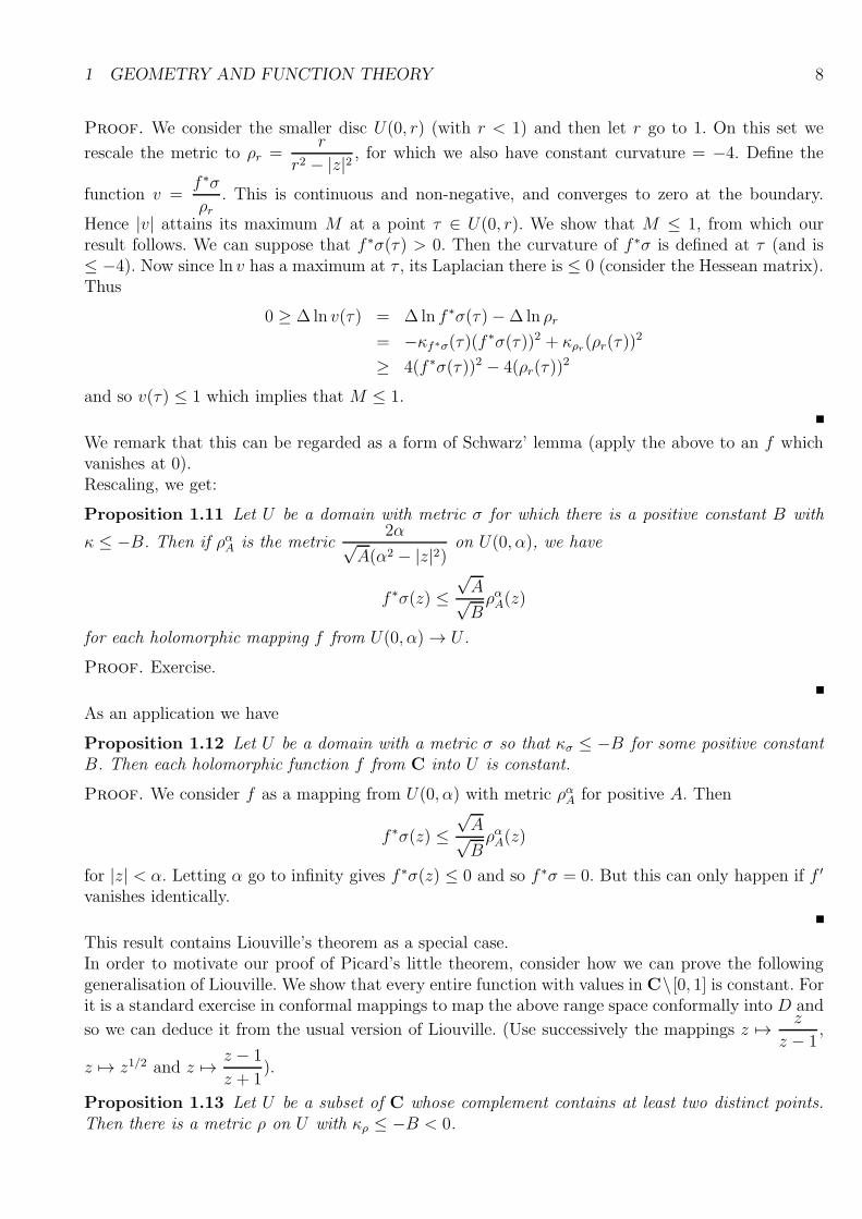
Proof. We consider the smaller disc U(0, r) (with r < 1) and then let r go to 1. On this set we
rescale the metric to ρr =r
r2 − |z|2 , for which we also have constant curvature = −4. Define the
function v =f ∗σ
ρr. This is continuous and non-negative, and converges to zero at the boundary.
Hence |v| attains its maximum M at a point τ ∈ U(0, r). We show that M ≤ 1, from which ourresult follows. We can suppose that f ∗σ(τ) > 0. Then the curvature of f ∗σ is defined at τ (and is≤ −4). Now since ln v has a maximum at τ , its Laplacian there is ≤ 0 (consider the Hessean matrix).Thus
0 ≥ ∆ ln v(τ) = ∆ ln f ∗σ(τ)−∆ ln ρr
= −κf∗σ(τ)(f∗σ(τ))2 + κρr(ρr(τ))
2
≥ 4(f ∗σ(τ))2 − 4(ρr(τ))2
and so v(τ) ≤ 1 which implies that M ≤ 1.
We remark that this can be regarded as a form of Schwarz’ lemma (apply the above to an f whichvanishes at 0).Rescaling, we get:
Proposition 1.11 Let U be a domain with metric σ for which there is a positive constant B with
κ ≤ −B. Then if ραA is the metric2α√
A(α2 − |z|2)on U(0, α), we have
f ∗σ(z) ≤√A√BραA(z)
for each holomorphic mapping f from U(0, α)→ U .
Proof. Exercise.
As an application we have
Proposition 1.12 Let U be a domain with a metric σ so that κσ ≤ −B for some positive constantB. Then each holomorphic function f from C into U is constant.
Proof. We consider f as a mapping from U(0, α) with metric ραA for positive A. Then
f ∗σ(z) ≤√A√BραA(z)
for |z| < α. Letting α go to infinity gives f ∗σ(z) ≤ 0 and so f ∗σ = 0. But this can only happen if f ′
vanishes identically.
This result contains Liouville’s theorem as a special case.In order to motivate our proof of Picard’s little theorem, consider how we can prove the followinggeneralisation of Liouville. We show that every entire function with values in C\ [0, 1] is constant. Forit is a standard exercise in conformal mappings to map the above range space conformally into D and
so we can deduce it from the usual version of Liouville. (Use successively the mappings z 7→ z
z − 1,
z 7→ z1/2 and z 7→ z − 1
z + 1).
Proposition 1.13 Let U be a subset of C whose complement contains at least two distinct points.Then there is a metric ρ on U with κρ ≤ −B < 0.
1 GEOMETRY AND FUNCTION THEORY 9
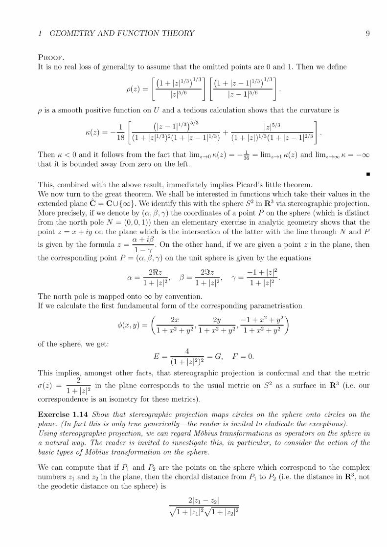
Proof.
It is no real loss of generality to assume that the omitted points are 0 and 1. Then we define
ρ(z) =
[
(
1 + |z|1/3)1/3
|z|5/6
][
(
1 + |z − 1|1/3)1/3
|z − 1|5/6
]
.
ρ is a smooth positive function on U and a tedious calculation shows that the curvature is
κ(z) = − 1
18
[
(
|z − 1|1/3)5/3
(1 + |z|1/3)2(1 + |z − 1|1/3) +|z|5/3
(1 + |z|)1/3(1 + |z − 1|2/3
]
.
Then κ < 0 and it follows from the fact that limz→0 κ(z) = − 136
= limz→1 κ(z) and limz→∞ κ = −∞that it is bounded away from zero on the left.
This, combined with the above result, immediately implies Picard’s little theorem.We now turn to the great theorem. We shall be interested in functions which take their values in theextended plane C = C∪∞. We identify this with the sphere S2 in R3 via stereographic projection.More precisely, if we denote by (α, β, γ) the coordinates of a point P on the sphere (which is distinctfrom the north pole N = (0, 0, 1)) then an elementary exercise in analytic geometry shows that thepoint z = x+ iy on the plane which is the intersection of the latter with the line through N and P
is given by the formula z =α + iβ
1− γ. On the other hand, if we are given a point z in the plane, then
the corresponding point P = (α, β, γ) on the unit sphere is given by the equations
α =2ℜz
1 + |z|2 , β =2ℑz
1 + |z|2 , γ =−1 + |z|21 + |z|2 .
The north pole is mapped onto ∞ by convention.If we calculate the first fundamental form of the corresponding parametrisation
φ(x, y) =
(
2x
1 + x2 + y2,
2y
1 + x2 + y2,−1 + x2 + y2
1 + x2 + y2
)
of the sphere, we get:
E =4
(1 + |z|2)2 = G, F = 0.
This implies, amongst other facts, that stereographic projection is conformal and that the metric
σ(z) =2
1 + |z|2 in the plane corresponds to the usual metric on S2 as a surface in R3 (i.e. our
correspondence is an isometry for these metrics).
Exercise 1.14 Show that stereographic projection maps circles on the sphere onto circles on theplane. (In fact this is only true generically—the reader is invited to eludicate the exceptions).Using stereopgraphic projection, we can regard Mobius transformations as operators on the sphere ina natural way. The reader is invited to investigate this, in particular, to consider the action of thebasic types of Mobius transformation on the sphere.
We can compute that if P1 and P2 are the points on the sphere which correspond to the complexnumbers z1 and z2 in the plane, then the chordal distance from P1 to P2 (i.e. the distance in R3, notthe geodetic distance on the sphere) is
2|z1 − z2|√
1 + |z1|2√
1 + |z2|2
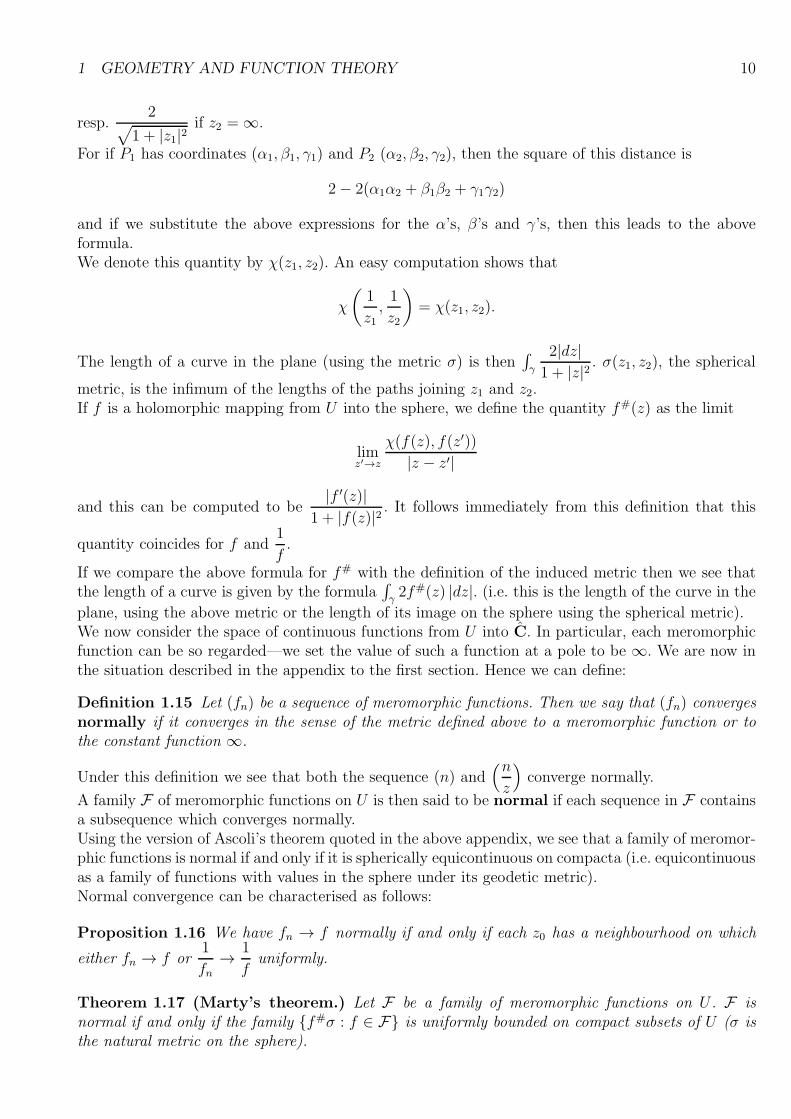
1 GEOMETRY AND FUNCTION THEORY 10
resp.2
√
1 + |z1|2if z2 =∞.
For if P1 has coordinates (α1, β1, γ1) and P2 (α2, β2, γ2), then the square of this distance is
2− 2(α1α2 + β1β2 + γ1γ2)
and if we substitute the above expressions for the α’s, β’s and γ’s, then this leads to the aboveformula.We denote this quantity by χ(z1, z2). An easy computation shows that
χ
(
1
z1,1
z2
)
= χ(z1, z2).
The length of a curve in the plane (using the metric σ) is then∫
γ
2|dz|1 + |z|2 . σ(z1, z2), the spherical
metric, is the infimum of the lengths of the paths joining z1 and z2.If f is a holomorphic mapping from U into the sphere, we define the quantity f#(z) as the limit
limz′→z
χ(f(z), f(z′))
|z − z′|
and this can be computed to be|f ′(z)|
1 + |f(z)|2 . It follows immediately from this definition that this
quantity coincides for f and1
f.
If we compare the above formula for f# with the definition of the induced metric then we see thatthe length of a curve is given by the formula
∫
γ2f#(z) |dz|. (i.e. this is the length of the curve in the
plane, using the above metric or the length of its image on the sphere using the spherical metric).We now consider the space of continuous functions from U into C. In particular, each meromorphicfunction can be so regarded—we set the value of such a function at a pole to be ∞. We are now inthe situation described in the appendix to the first section. Hence we can define:
Definition 1.15 Let (fn) be a sequence of meromorphic functions. Then we say that (fn) convergesnormally if it converges in the sense of the metric defined above to a meromorphic function or tothe constant function ∞.
Under this definition we see that both the sequence (n) and(n
z
)
converge normally.
A family F of meromorphic functions on U is then said to be normal if each sequence in F containsa subsequence which converges normally.Using the version of Ascoli’s theorem quoted in the above appendix, we see that a family of meromor-phic functions is normal if and only if it is spherically equicontinuous on compacta (i.e. equicontinuousas a family of functions with values in the sphere under its geodetic metric).Normal convergence can be characterised as follows:
Proposition 1.16 We have fn → f normally if and only if each z0 has a neighbourhood on which
either fn → f or1
fn→ 1
funiformly.
Theorem 1.17 (Marty’s theorem.) Let F be a family of meromorphic functions on U . F isnormal if and only if the family f#σ : f ∈ F is uniformly bounded on compact subsets of U (σ isthe natural metric on the sphere).
1 GEOMETRY AND FUNCTION THEORY 11
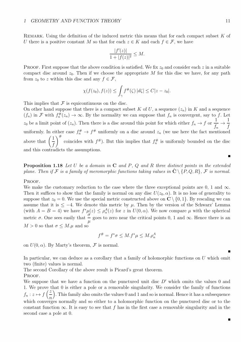
Remark. Using the definition of the induced metric this means that for each compact subset K ofU there is a positive constant M so that for each z ∈ K and each f ∈ F , we have
|f ′(z)|1 + |f(z)|2 ≤M.
Proof. First suppose that the above condition is satisfied. We fix z0 and consider each z in a suitablecompact disc around z0. Then if we choose the appropriate M for this disc we have, for any pathfrom z0 to z within this disc and any f ∈ F ,
χ(f(z0), f(z)) ≤∫
γ
f#(ζ) |dζ | ≤ C|z − z0|.
This implies that F is equicontinuous on the disc.On other hand suppose that there is a compact subset K of U , a sequence (zn) in K and a sequence(fn) in F with f#
n (zn) → ∞. By the normality we can suppose that fn is convergent, say to f . Let
z0 be a limit point of (zn). Then there is a disc around this point for which either fn → f or1
fn→ 1
funiformly. In either case f#
n → f# uniformly on a disc around zn (we use here the fact mentioned
above that
(
1
f
)#
coincides with f#). But this implies that f#n is uniformly bounded on the disc
and this contradicts the assumptions.
Proposition 1.18 Let U be a domain in C and P , Q and R three distinct points in the extendedplane. Then if F is a family of meromorphic functions taking values in C \ P,Q,R, F is normal.
Proof.
We make the customary reduction to the case where the three exceptional points are 0, 1 and ∞.Then it suffices to show that the family is normal on any disc U(z0, α). It is no loss of generality tosuppose that z0 = 0. We use the special metric constructed above on C \ 0, 1. By rescaling we canassume that it is ≤ −4. We denote this metric by µ. Then by the version of the Schwarz’ Lemma(with A = B = 4) we have f ∗µ(z) ≤ ρAα (z) for z in U(0, α). We now compare µ with the spherical
metric σ. One sees easily thatσ
µgoes to zero near the critical points 0, 1 and ∞. Hence there is an
M > 0 so that σ ≤M.µ and so
f# = f ∗σ ≤M.f ∗µ ≤M.ρAα
on U(0, α). By Marty’s theorem, F is normal.
In particular, we can deduce as a corollary that a family of holomorphic functions on U which omittwo (finite) values is normal.The second Corollary of the above result is Picard’s great theorem.Proof.
We suppose that we have a function on the punctured unit disc D′ which omits the values 0 and1. We prove that 0 is either a pole or a removable singularity. We consider the family of functions
fn : z 7→ f( z
n
)
. This family also omits the values 0 and 1 and so is normal. Hence it has a subsequence
which converges normally and so either to a holomorphic function on the punctured disc or to theconstant function ∞. It is easy to see that f has in the first case a removable singularity and in thesecond case a pole at 0.
1 GEOMETRY AND FUNCTION THEORY 12
1.4 Appendix
Definition 1.19 Norm, seminorm, normed space Banach space , locally convex space, Frechet space.
In the first paragraph, we introduce the basic definitioins (normed spaces, isomorphisms, continuouslinear operators) and bring some classical examples (finite dimensional spaces, spaces of continuousand differentiable functions). We then present some basic facts on duality for normed spaces. The dualof a normed space is the space of continuous linear functionals acting on it and plays the same rolein the infinite dimensional theory as does the algebraic dual for finite dimensional spaces. However,as we shall see later, this duality does not possess the symmetry of the finite dimensional case—inparticular, a Banach space cannot always be identified in a natural way with its second dual. It isnot even obvious that the duality is non-trivial i.e. that there are always enough continuous linearfunctionals on a normed space. That this is in fact the case is a consequence of one of the most famousresults on normed spaces—the Hahn-Banach theorem, which is studied in detail in paragraph 2.In order to obtain deeper results of an analytic nature, a natural completeness condition must beimposed—that of completeness with respect to the metric induced by the norm. The spaces withthis properties are the Banach spaces. They are introduced in paragraph 3 and it is shown that theexamples introduced in the first paragraph are Banach spaces. In paragraph 4 we consider a famousgroup of closely related theorems which use the completenss in an essential way (via an applicationof Baire’s category theorem). They can each be regarded as precise statements of the vague principlethat if a linear mapping between Banach spaces can be constructed directly, it is continuous. In thefifth paragraph we introduce one of the most important groups of Banach spaces—the Lp-spaces. Forthe sake of completeness we begin with a brief survey of the basic concepts of measure theory. TheLp-spaces are then defined and their properties (completenss, duality etc.) are derived. Paragraph 6is devoted to Hilbert spaces i.e. those Banach space whose norms are defined by an inner product.Historically, these were the first Banach spaces to be studied intensively—by Hilbert in the contextof integral equations. We include a proof of his spectral theorem for compact, self-adjoint operatorswhich, together with its applications to differential equations (notably, Sturm-liouville problems),was an imporatant stage in the history of functional analysis. This leads naturally to the topic ofinfinite dimensional operators. Their structure can be exceedingly complicated and in the seventhparagraph we restrict attention to a class of operators whose behaviour is closest to that of the finitedimensional ones—the compact operators. It is shown that their spectrum has a particulalry simplestructure.Paragraph 8 is devoted to an introduction to one of the most important concepts in Banach spacetheory—that of a (Schauder) basis. An attempt has been made to show just how essential a tool thisis in investigations into the structure of conrete Banach spaces and their subspaces and quotients.A final section is devoted to some more subtle constructions on Banach space—infinite sums andproducts, tensor products and ultraproducts.I.1. Normed spaces: We begion with the elementary theory of normed spaces. These are vectorspaces with suitable distance functions. With the help of this distance, the usual procedures involvinglimit operations (approximation of non-linear operators by their derivatives, approximation methodsfor constructing solutions of equations etc.) can be carried out. Definition 1.1 below, which wasexplicitly introduced by Banach andWiener, was already implicit in earlier work on integral equationsby Riesz (who employed the concrete normed spaces C(I), Lp(I) which will be introduced below).The plan of the section is simple. We begin by introducing the two main concepts of the chapter—normed spaces and continuous linear operators. Their more obvious properties are discussed andsome concrete examples—mainly the so-called ℓp-spaces—are introduced.
Definition 1.20 Definition 1.1 A seminorm on a vector spaces E (over C or R) is a mappingx 7→ ‖x‖ from E into R+ with the properties
1 GEOMETRY AND FUNCTION THEORY 13
‖x+ y‖ ≤ ‖x‖+ ‖y‖ (x, y ∈ E);
‖λx‖ = |λ|‖x‖ (x ∈ E, λ ∈ C or R resp.;
‖ ‖ is a norm if, in addition, (3) ‖x‖ = 0 implies x = 0 (x ∈ E).Aa normed space is a pair (E, ‖ ‖) where E is a vector space and ‖ ‖ is a norm on E.If ‖ ‖ is a seminorm (resp. a norm) the mapping
d‖ ‖ : (x, y) 7→ ‖x− y‖
is a semimetric (res. a metric) on E. We call it the semimetric (metric) induced by ‖ ‖. Thusevey normed space (E, ‖ ‖) can be regarded in a natural way as a metric space and so as a topologicalspace and we can use, in the context of normed spaces, such notions as continuity of mappings,convergence of sequences or nets, compactness of subsets etc.If (E, ‖ ‖) is a normed space, we write B‖ ‖ or B(E) for the closed unit ball of E i.e. the set‖x ∈ E : ‖x‖ ≤ 1.
Exercise 1.21 A. A subset A of a vector space is absolutely convex if λx+ µy ∈ A wheneverx, y ∈ A, λ, µ ∈ C (respectivly R) and |λ|+ |µ| ≤ 1.
A is absorbing if for each x ∈ E there is a ρ > 0 so that λx ∈ A when ‖λ| ≤ ρ. Show thatB(E) is absolutly convex and absorbing and that if A is absolutely convex and absorbing, then
‖ ‖A : x 7→ infρ > 0 : x ∈ ρA
is a seminorm on E (it is called the Minkowski functional of A). Show that it is a norm ifand only if A contains no non-trivial subspace of E.
B. Let E be a vector space, A an absolutely convex subset which does not contain a non-trivialsubspace. Let EA =
⋃
n∈N nA. Show
that EA is a vector subspace of E;
that A absorbs EA;
that (E, ‖ ‖A) is a normed space.
The usual constructions (products, subspaces, quotients etc.) can be carried out in the context ofnormed spaces. For examples, if G is a vector subspace of the normed space (E, ‖ ‖), the restriction‖ ‖G of ‖ ‖ to G is a norm thereon and we we can regard G in a natural way as a normed space (thisnorm is called the norm induced on G by ‖ ‖).Similarly, if πG denotes the natural projection from E onto the quotient space E/G, then the mapping
y 7→ inf‖x‖ : x ∈ E and πG = y
is a seminorm. The question of when it is a norm is examined in an exercise below.There are several possibilities for defining norms on product spaces and we shall discuss these insome detail later. For our purposes, the following one on a product of two spaces will suffice: let(E, ‖ ‖1) and (F, ‖ ‖2) be normed spaces. The mapping
(x, y) 7→ max‖x‖1, ‖y‖2
is a norm on E × F which (with this norm) is then called the normed product of E and F . (Notethat the unit ball of E × F is then just the Cartesian product of the unit balls of E and F ).
1 GEOMETRY AND FUNCTION THEORY 14
Exercise 1.22 1. Show that the topology induced by ‖ ‖G on G coincides with the restriction toG of the topology of E;
2. if x ∈ E, show that ‖piG(x)‖ (the norm in E/G) is just the distance from x to G i.e. inf‖x−y‖ :y ∈ G. Deduce that the seminorm on E/G is a norm if and only if G is closed. Use this togive an example where it is not a norm.
3. Show that the topology induced by the norm on E×F is the product of the topologies on E andF .
It follows from the very definition of the topology via the norm that it is very closely related to thelinear structure of E. In fact, the following properties are valid:
1. the mappings A : (x, y) 7→ x+ y and M : (λ, x) 7→ λx from E ×E → E resp. C×E or R×Eto E are continuous for the topology generated by the norms. For
‖(x+ y)− (x1 + y1)‖ ≤ ‖x− x1‖+ ‖y − y1‖
and‖λx− λ1x1‖ ≤ |λ− λ1|‖x‖+ |λ1|‖x− x1‖.
2. Let G be a subspace of (E, ‖ ‖). Then the closure G of G is also a subspace.
Exercise 1.23 Let ‖ ‖ be a seminorm on E. Show that E0 = x ∈ E : ‖x‖ = 0 is a subspace ofE. If π0 denotes the natural projection from E onto E/E0, show that π0(x) 7→ ‖x‖ is a well-definedmapping on E/E0 and is, in fact, a norm. E/E0, with this norm, is called the normed spaceassociated with E. (This simple exercise is often useful on occasions when a natural construction“should” produce a normed space but in fact only produces a seminormed one. We simply factor ourthe zero subspace).
As is customary in mathematics, we identify normed spaces which have the same structure. Theappropriate concept is that of an isomorphism. It turns out that there two natural ones in thiscontext:Let E and F be normed space. E and F are isomorphic if there is a bijective linear apping T : E → Fso that T is a homeomorphism for the norm topologies. T is then called an isomorphism. If T is,in addition, norm-preserving (i.e. ‖Tx‖ = ‖x‖ for x ∈ E) T is an isometry and E and F areisometrically isomorphic (we write E ∼ F to indicate that E and F are isomorphic).Two norms ‖ ‖ and ‖ ‖1 on a vctor space E are equivalent if IdE is an isomorphism from (E, ‖ ‖)onto (E, ‖ ‖1) i.e. if ‖ ‖ and ‖ ‖1 induce the same topology on E. Isomorphisms are characterised bythe existence of estimates from above and below: let T : E → F be a bijective linear mapping. ThenT is an isomorphism if and only if there exist M and m (both positive) so that
m‖x‖ ≤ ‖Tx‖ ≤M‖x‖ (x ∈ E).
(For a proof see Exercise 1.8 below).Thus the norms ‖ ‖ and ‖ ‖1 on E are equivalent if and only if there are M,m > 0 so thatm‖x‖ ≤ ‖x‖1 ≤M‖x‖ (x ∈ E).We now bring a list of some simple examples of normed space. In the course of the later cahpters weshall extend it considerably.
1 GEOMETRY AND FUNCTION THEORY 15
Exercise 1.24 A. The following mappings on Cn (resp. Rn) are norms:
‖ ‖1 : (ξ1, . . . , ξn) 7→ (|ξ1|+ · · ·+ |ξn|);‖ ‖2 : (ξ1, . . . , ξn) 7→ (|ξ1|2 + · · ·+ |ξn|2)1/2;‖ ‖∞ : (ξ1, . . . , ξn) 7→ max(|ξ1|, . . . , |ξn|).
Each of these norms induces the usual topology on Cn (res. Rn). Note that the respective unitballs are (for n = 3) the octahedron, the euclidean ball and the cube (or hexahedron).
B. Let K be a compact space. C(K) denotes the space of continuous, complex-valued functions onK. This space has a natural vector space structure and the mapping
‖ ‖∞ : x 7→ sup|x(t)| : t ∈ K
is a norm. ‖ ‖∞ induces the topology of uniform convergence on K (that is, a sequence or netof functions in C(K) is norm-convergent if and only if it is uniformly convergent on K).
C. let I be a compact interval in R, n a positive integer. The space
Cn(I) = x ∈ C(I) : x, x′, . . . , x(n) exist and are continuous
has a natural vector space structure and the mapping
‖ ‖n∞x 7→ max‖x‖∞, . . . , ‖x(n)‖∞
is a norm on Cn(I). Note that Cn(I) is a vector subspace of C(I) but that (Cn(I), ‖ ‖n∞) is anot a normed subspace of (C(I), ‖ ‖∞)—that is ‖ ‖n∞ is not the norm induced on Cn(I) fromC(I)—or even equivalent to it.
D. Let (Ek, ‖ ‖k) : k = 1, . . . , n be a family of normed spaces. On the product E =∏n
k=1 wedefine two norms:
‖ ‖s : (x1, . . . , xn) 7→n∑
k=1
‖xk‖k;
‖ ‖∞ : (x1, . . . , xn) 7→n
maxk=1‖xk‖k.
Then ‖ ‖s and ‖ ‖∞ are distinct norms on E (if n > 1) which are, however, equivalent. Infact, we have the inequality: ‖x‖∞ ≤ ‖x‖s ≤ n‖x‖∞ (note that this means geometrically thatthe unit ball of ‖‖s is containd in that of ‖ ‖∞ resp. contains a copy of it reduced by a factor1
n).
Exercise 1.25 A. ? at on C([0, 1]), the mapping x 7→∫ 1
0|x(t)| dt is a norm which is not equivalent
to ‖ ‖∞.
B. Show that the mapping x 7→ (x, x′, . . . , x(n)) is an isomorphism from Cn(I) onto a subspace ofthe product space C(I)× · · · × C(I) ((n+ 1) factors).
An important role in the thoery of infinite dimensional spaces is played by linear operators. Incontrast to the finite dimensional case, we impose the following condition, which takes account ofthe topological resp. norm structure:
1 GEOMETRY AND FUNCTION THEORY 16
Definition 1.26 A linear mapping T : ((E, ‖‖1)→ (F, ‖ ‖2) is bounded if there is a C > 0 so that‖Tx‖2 ≤ C‖x‖1 (x ∈ E).
In fact, this is equivalent to continuity. Indeed we have equivalence of the following three conditionson a linear operator T between normed space E and F :
T is continuous;
T is continuous at 0;
T is bounded.
Proof. 1) implies 3) is immediate. 2) implies 3): since T is continuous at 0 and B(F ) is a neigh-bourhood of 0 = T (0), there is a positive δ so that Tx ∈ B(F ) if ‖x‖1 < δ. Now for each x ∈ E with
x non-zero,
∥
∥
∥
∥
δx
‖x‖1
∥
∥
∥
∥
1
≤ δ and so
∥
∥
∥
∥
T
(
δx
‖x‖1
)∥
∥
∥
∥
1
≤ δ i.e. ‖Tx‖2 ≤‖x‖1δ
. 3) implies 1): we suppose
that C is chosen as in 1.7. Then
‖Tx− Ty‖2 = ‖T (x− y)‖2 ≤ C‖x− y‖1
and so T is even Lipschitz continuous.
We write L(E, F ) for the set of bounded linear mappings from E into F . This space has a naturalvector space structure (via pointwise addition and multiplication by scalars). We define a norm onit as follows:
‖T‖ = infC > 0 : ‖Tx‖2 ≤ C‖x‖1 (x ∈ E).If E, F and G are normed spaces and T ∈ L(E, F ) and S ∈ L(F,G), then the composed mappingST is also bounded and we have the estimate ‖ST‖ ≤ ‖S‖‖T‖ for its norm.
Exercise 1.27 A. Use 1.7 to obtain the characterisatio of isomorphisms given before 1.5.
B . Show that the formula given above does indeed define a norm on L(E, F ) and that
‖T‖ = sup‖Tx‖2‖x‖1: x ∈ E, x 6= 0
= sup‖Tx‖2 : x ∈ B(E) = sup‖Tx‖2 : ‖x‖1 = 1.
C. A subset of a normed space E is bounded if the norm is bounded on it. Show that this isequivalent to the fact that the set C is absorbed by the unit ball (i.e. there is a K > 0 so thatC ⊂ KBE). Show that a linear mapping T between normed spaces is bounded if and only if itmaps bounded sets into bounded sets and that a subset of L(E, F ) is bounded if and only if itis equicontinuous.
Example 1.28 We bring some basic examples of operatoors:
A. Let A = [aij ] be an m× n matrix. Then the coresponding linear mapping
TA : (ξj) 7→(
n∑
j=1
aijξj
)m
i=1
is bounded from (Rn, ‖ ‖p) into Rm, ‖ ‖p) for p = 1, 2 or infty
1 GEOMETRY AND FUNCTION THEORY 17
B. We define a mapping D : C1(I) → C(I) by D : x 7→ x′. D is linear and bounded (in fact‖D‖ ≤ 1). More generally, one can define the operator Dk of k-times differentiation which canbe regarded as a continuous linear mapping from Cn+k(I)intoCn(I).
C. Let a be a function in C(I). Then the mapping Ma : x 7→ ax is continuous and linear on C(I)and ‖Ma‖ ≤ ‖a‖∞. D. Differential operators: let a0, . . . , an be elements of C(I). Then we definea differential operator L : Cn(I)→ C(I) by L =
∑nk=0Mak Dk.
E. Let K be a bounded, continuous complex-valued function on I × J (I, J compact intervals inR). We define the integral operator IK with kernel K as follows:
IK : x 7→ (s 7→∫
J
K(s, t)x(t) dt.
IK is a continuous linear mapping from C(J) into C(I). F. (Projections) An operator T ∈ L(E)is a projection if T 2 = T . Then Id− T is also a projection (since
(Id− T )2 = Id− 2T + T 2 = Id− T ).
Also T (E) = x : Tx = x = Ker (Id− T ) and so is closed.
The standard example of a projection is the mapping (x, y) 7→ (x, 0) from a product space E1 × E2
onto the factor E2. In a sense this is the only one since if T ∈ L(E) is a projection, then the mappingx 7→ (Tx, (Id − T )x) is an algebraic isomorphism from E onto the product space E1 × E2 whereE1 = T (E), E2 = (Id − T )(E). In fact, it is also an isomorphism for the norm structure on theproduct. Hence a projection in this case causes a splitting up of the space into a product. A subspaceof E is complemented if it is the range of a projection T ∈ L(E). E is then simultaneously asubspace of E and also isomorphic to a quotient space.
Exercise 1.29 A. Let A = [aij ] be as in 1.9.A and consider TA as a mapping from (Rn, ‖ ‖infty)into (Rn, ‖ ‖∞). Show that ‖TA‖ = supi
∑nj=1 |aij|. What is its norm as an operator for the
norms ‖ ‖1 and ‖ ‖2?
B. Show that ‖D‖ = 1 and that ‖Ma‖ = ‖a‖∞. Give an estimate for the norms of L and IK(notation as in 1.9.B - E).
C. Let E and F be normed spaces, G a closed subspace of E, T a bounded linear operator from Einto F . Show that if T (G) = ‖0‖, then it can be lifted to a continuous linear operator T fromE/G into F (i.e. T is such that T πG = T ).
We shall be interested in the following properties of mappings T ∈ L(E, F ):
injectivity: this means that KerT = 0;surjectivity: i.e. that T (E) = F ;
bijectivity: i.e. injectivity and surjectivity;
isomorphicity: c.f. definition after 1.4 above;
existence of a right inverse i.e. an S ∈ L(E, F ) so that TS = IdF ;
existence of a left-inverse i.e. an S ∈ L(E, F ) so that ST = IdE .
1 GEOMETRY AND FUNCTION THEORY 18
Note that for a linear operator T on a finite dimensional space E, all of these notions coincide. Inthe infinite dimensional case, this is no longer true. We shall give some examples here and later.In connection with these definitions, we can give various generalisations of the notion of an eigenvalueof an operator. We shall begin here with the most useful one. Later we shall consider refinements.If T ∈ L(E), the spectrum of T is the set of those λ ∈ C for which (λId−T ) is not an isomorphism.To illustrate these concepts, consider the following examples:
A. The identity mapping from C([0, 1]) (with the supremum norm) into the same space with the
norm ‖x‖1 =∫ 1
0|x(t)| dt is a bijection but not an isomorphism.
B. The operator Ma on C([0, 1]) is injective if and only if the set of zeroes of a has empty interior.It is surjective if and only if a has no zeroes. In the latter case it is an isomorphism. Thespectrum of Ma is the range of a. A generalisation of the concept of a linear mapping whichis often useful is that of a multi-linear mapping whereby T :
∏nk=1Ek → F (the spaces being
vector spaces) is multilinear if for each i, the partial mapping
x 7→ T (x1, . . . , xi−1, x, xi+1, . . . , xn)
is linear for any choice of x1, . . . , xi−1, xi+1, . . . , xn.
The space of multilinear mappings is denoted by L(E∞, . . . , E\;F). It has a natural linear structure.If the E’s and F are normed spaces then the following conditions on such a maapping T are easilyseen to be equivalent:
T is continuous as a mapping from∏n
k=1Ek with the product topology into F ;
T is bounded i.e. there is a C > 0 so that
‖T (x1, . . . , xN)‖ ≤ C‖x1‖ . . . ‖xn‖for each x1, . . . , xn.
This is proved exactly as for linear mappings.The space of such multilinear mappings is denoted by L(E1, . . . , En;F ). It is a linear subspace ofL(E∞, . . . , E\;F) and the mapping
T 7→ sup‖T (x1, . . . , xn)‖ : xi ∈ BEi‖
is a norm thereon. The case F = R (resp. (C) is particularly important and then we write L(E∞∞, . . . , E\)and L(E1, . . . , En) for the corresponding spaces.In applications we usually have the situation where all of the Ei are equal to a given space E. In thiscase we write Ln(E;F ) resp. Ln(E) for the corresponding space.Typical examples of such multilinear mappings are tensors (in the finite dimensional case) or map-pings of the form
(x1, . . . , xn) 7→∫
. . .
∫
x1(s1) . . . xn(sn) ds1 . . . dsn
on C([0, 1]) where K is a suitable kernel e.g. a continuous function on [0, 1]n.In the theory of differentiation for funtions between Banach space, we shall encounter “nested” spacesof linear operators such as L(E,L(E, F )), L(E,L(E,L(E, F ))) etc. Fortunately, these can be moreconveniently represented by spaces of multilinear mappings as the following proposition shows:
Proposition 1.30 The mapping
T 7→ (x1 7→ ((x2, . . . , xn) 7→ T (x1, . . . , xn)
is a linear isometric isomoprhism from L(E1, . . . , En;F ) onto L(E1, L(E2, . . . , En;F )).
1 GEOMETRY AND FUNCTION THEORY 19
Proof. We prove this for the case n = 2. First note that the mapping S : ((x1, x2) 7→ (Sx1)(x) isan inverse for the one in the statement of the theorem. That both are isometries follows from theequality:
‖T‖ = sup‖T (x1, x2)‖ : ‖x2‖ ≤ 1, ‖x2‖ ≤ 1= sup
‖x1‖≤1
sup‖T (x1, x2)‖ : ‖x2‖ ≤ 1.
If we apply this result repeatedly, we see that the nested space L(E1, L(E2, . . . , L(En, F ) . . . ) isisometrically isomorphic to L(E1, . . . , En;F ), in particular to Ln(E;F ) in the case where all of theEi coincide with E.We continue this section with some remarks on finite dimensional spaces. These have played anincreasingly important role in the theory of normed spaces in recent years as building blocks forinfinite dimensional ones. They are also very helpful in providing a geometrical intuition which isuseful even in the infinite dimensional case.The first result shows that, as far as the topological structutre is concerned, all finite dimensio-nal spaces (of the same dimension) are the same. We emphasise, however, that the isometric resp.geometric properties are very distinct.
Proposition 1.31 Every real, finite dimensional normed space E is isomorphic to (Rn, ‖ ‖∞) wheren = dimE. Similarly, every n-dimensional normed space over C is isomorphic to (Cn, ‖ ‖∞).
Proof. Let (x1, . . . , xn) be a basis for E and consider the continuous linear map
T : (λ1, . . . , λn) 7→n∑
i=1
λixi
from Rn → E.The image of the unit sphere of Rn under T is a compact subset of E which does not contain 0 (sincethe xi are linearly independent). Hence there is a δ > 0 so that ‖T (λ)‖ ≥ δ if λ ∈ Rn, ‖λ‖∞ = 1 (sincea continuous function on a compact set attains its infimum). From this it follows that ‖T−1‖ ≤ 1/δ.The complex case can be proved similarly.
Corollary 1.32 Any two norms on a finite dimensional normed space are equivalent.
We shall now develop the generalisation of the concept of Banach spaces which is relevant as aframework for the topological structure of spaces of test functions and distributions. Typically theformer are spaces of functions which are submitted to an infinite number of conditions, usually ofgrowth and regularity. The appropriate concept is that of a locally convex topology i.e. one which isdefined by a family of seminorms rather than by a single norm.Recall that a seminorm on a vector space E is a mapping p from E into the non-negative reals sothat
p(x+ y) ≤ p(x) + p(y) p(λx) = |λ|p(x)for each x, y in E and λ in R.We shall use letters such as p, q to denote seminorms. The family of all seminorms on E is orderedin the natural way i.e. p ≤ q if p(x) ≤ q(x) for each x in E. If p is a seminorm,
Up = x ∈ E : p(x) ≤ 1
1 GEOMETRY AND FUNCTION THEORY 20
is the closed unit ball of p. This is an absolutely convex, absorbing subset of E, whereby a subsetA of E is convex if for each x, y ∈ A and t ∈ [0, 1], tx+ (1 − t)y ∈ A balanced if λA ⊂ A for λ inR with |λ| ≤ 1 absolutely convex if it is convex and balanced; absorbing if for each x in E thereis a positive ρ so that λx ∈ A for each λ with |λ| < ρ. Up is in addition algebraically closed i.e. itsintersection with each one-dimensional subspace of E is closed, whereby these subspaces carry thenatural topologies as copies of the line. On the other hand, ifU is an absolutely convex, absorbingsubset of E, then its Minkowski functional i.e. the mapping
pU : x 7→ infλ > 0 : x ∈ λU
is a seminorm on E. In fact, the mapping p 7→ Up is a one-one correspondence between the set ofseminorms on E and the set of absolutely convex, absorbing, algebraically closed subsets of E. Alsop ≤ q if and only if Up ⊂ Uq.A family S of seminorms on E is irreducible if the following conditions are verified:
a) if p ∈ S and λ ≥ 0, then λp ∈ S;
b) if p ∈ S and q is a seminorm on E with q ≤ p, then q ∈ S;
c) if p1 and p2 are in S, then so is max(p1, p2);
d) S separates E i.e. if x is a non-zero element of E, then there is a p ∈ S with p(x) 6= 0.
If S is a family of seminorms which satisfies only d), then there is a smallest irreducible family ofseminorms which contains S. It is called the irreducible hull of S and denoted by S. (S is theintersection of all irreducible families containing S – alternatively it consists of those seminormswhich are majorised by one of the form
max(λ1p1, . . . , λnpn)
where the λi’s are positive scalars and the pi’s are in S).A locally convex space is a pair (E, S) where E is a vector space and S is an irreducible family ofseminorms on the former. If S is a family of seminorms which separates E, then the space (E, S) isthe locally convex space generated by S.If (E, S) is a locally convex space, we define a topology τS on E as follows: a set U is said to be aneighbourhood of a in E if (U−a) contains the unit ball of some seminorm in S. The correspondingtopology is called the topology associated with S. This topology is Hausdorff (since S separatesE) and, in fact, completely regular, since it is generated by the uniformity which is defined by thesemimetrics (dp : p ∈ S) where dp(x, y) = p(x− y). Hence we can talk of convergence of sequences ornets, continuity and completeness in the context of locally convex spaces.Recall that a topological vector space is a vector space E together with a Hausdorff topology sothat the operations of addition and multiplication by scalars are continuous. It is easy to see that alocally convex space is a topological vector space. On the other hand, locally convex spaces are oftendefined as topological vector spaces in which the set of absolutely convex neighbourhoods of zeroforms a neighbourhood basis. This is equivalent to our definition. For if (E, S) is a locally convexspace as defined above, then (E, τS) is a topological vector space and the family Up : p ∈ S is abasis of convex neighbourhoods of zero. On the other hand, if (E, τ) is a topological vector spacesatisfying the convexity condition, then the set of all τ -continuous seminorms on E is irreducible andthe corresponding topology τS coincides with τ .We remark that if a family S of seminorms on the vector space E satisfies conditions a) - c) above,but not necessarily d) and we define
NS = x ∈ E : p(x) = 0, p ∈ S
1 GEOMETRY AND FUNCTION THEORY 21
then we can define a natural locally convex structure on the quotient space E/NS. This is a convenientmethod for dealing with non-Hausdorff spaces which sometimes arise.Examples:
I. Of course, normed spaces are examples of locally convex space, where we use the single normto generate a locally convex structure.
II. If E is a normed space and F is a separating subspace of its dual E ′, then the latter inducesa family S of seminorms, namely those of the form px : x 7→ |f(x)| for f ∈ F . This induces alocally convex structure on E which we denote by Sw(F ). The corresponding topology σ(E, F ) iscalled the weak topology induced by F . The important cases are where F = E ′, respectivelywhere E is the dual G′ of a normed space and F is G (regarded as a subspace of E ′ = G′′).
III. (the fine locally convex structure): If E is a vector space, then the set of all seminorms on Edefines a locally convex structure on E which we call the fine structure for obvious reasons.
IV. The space of continuous functions: If S is a completely regular space, we denote by K(S) orsimply by K, the family of all compact subsets of S. If K ∈ K, then
pK(x) = sup|x(t)| : t ∈ K
is a seminorm on C(S), the space of continuous functions from S into R. The family of all suchseminorms defines a locally convex structure SK on C(S) – the corresponding topology is thatof compact convergence i.e. uniform convergence on the compacta of S.
V. Differentiable functions. If k is a positive integer, Ck(R) denotes the family of all k-timescontinuously differentiable functions on R. For each r ≤ k and K in K(R), the mapping
prK : x 7→ sup|x(r)(t)| : t ∈ K
is a seminorm on Ck(R). The family of all such seminorms defines a locally convex structureon Ck(R).
VI. Spaces of operators: Let H be a Hilbert space. On the operator space L(H), we consider thefollowing seminorms:
px : T 7→ ‖Tx‖p∗x : T 7→ ‖T ∗x‖
px,y : T 7→ |(Tx|y)|for x and y in H . The family of all seminorms of the first type define the strong locallyconvex structure on L(H), while those of the first two type define the strong *-structure.Finally, those of the third type define the weak operator structure.
VI. Dual pairs. We have seen that the duality between a normed space and its dual can be used todefine weak topologies on E and E ′. For our purposes, a more symmetrical framework for suchduality is desirable. Hence we consider two vector spaces E and F , together with a bilinearform (x, y) 7→ 〈x, y〉 from E × F into R, which is separating i.e. such that
if y ∈ F is such that 〈x, y〉 = 0 for each x in E, then y = 0;;
if x ∈ E is such that 〈x, y〉 = 0 for each y in F , then x = 0.
1 GEOMETRY AND FUNCTION THEORY 22
Then we can regard F as a subspace of E∗, the algebraic dual of E, by associating to each yin F the linear functional
x 7→ 〈x, y〉.Similarly, E can be regarded as a subspace of F ∗. (E, F ) is then said to be a dual pair. Thetypical example is that of a normed space, together with its dual or, more generally, a subspaceof its dual which separates E. For each y ∈ F , the mapping py : x 7→ |〈x, y〉| is a seminorm onE and the family of all such seminorms generates a locally convex structure which we denoteby Sw(F ) – the weak structure generated by F .
A subset B of F is said to be bounded for the duality if for each x in E,
sup|〈x, y〉| : y ∈ B <∞.
In this case, the mappingpB : x 7→ suppy(x) : y ∈ B
is a seminorm on E. Let B denote a family of bounded subsets of F whose union is the whole ofF . Then the family pB : B ∈ B generates a locally convex structure SB on E, that of uniformconvergence on the subsets of B.Thus if B consists of the singletons of F , we rediscover the weak structure. If B is taken to be thefamily of those absolutely convex subsets of F which are compact for the topology defined by Sw(E)on F , then SB is called the mackey structure and the corresponding topology (which is denotedby τ(E, F )) is called the Mackey topology. Finally, if we take for B the family of all boundedsubsets of F , then we have the strong structure–the corresponding topology is called the strongtopology.A rich source of dual pairs is provided by the so-called sequence spaces. These are, by definition,subspaces of the space ω = RN i.e. the family of all real-valued sequences which contain φ, the spacesof those sequences with finite support (i.e. φ = x ∈ ω : ξn = 0 except for finitely many n.φ and ω are regarded as locally convex spaces, ω with the structure defined by the seminormspn : x 7→ |ξn| and φ with the fine structure.Further examples of sequence spaces are the ℓp-spaces.If E is a sequence space, we define its α-dual Eα as follows:
Eα = y = (ηn) :∑
|ξnηn| <∞ for each x ∈ E.
Then (E,Eα) is a dual pair under the bilinear form
〈x, y〉 =∞∑
n=1
ξnηn.
Of course, if E ⊂ F , then Eα ⊃ F α. Also E is clearly a subspace of (Eα)α). A sequence space E isperfect if E = Eαα. Thus
ωα = φ φα = ω (ℓp)α = ℓq
the latter for all values of p and q. Hence all of these spaces are perfect.In particular, ℓ2 is self-dual i.e. equal to its own α-dual. In fact, this is a characterisation of ℓ2 as thereader can verify. More precisely, if a sequence space E is such that E = Eα, then E = ℓ2.The β-dual of E is the family of those sequences y = (ηn) for which
∑
ξnηn converges for each x ∈ E.This coincides with the α-dual when E is solid i.e. such that whenever x ∈ E and z is dominated byx i.e. |ζn| ≤ |ξn| for each n, then z ∈ E.
1 GEOMETRY AND FUNCTION THEORY 23
As in the case of normed spaces, we are interested in linear mappings between locally convex spaceswhich preserve their topological structures. Corresponding to the fact that boundedness and conti-nuity are equivalent for linear mappings between normed spaces, we have the following equivalences:for a linear mapping T : E → F whereby (E, S) and (F, S1) are locally convex spaces, the followingare equivalent:
T is τS − τS1-continuous;
T is τS − τS1-continuous at zero;
for each p ∈ S1, p T ∈ S;
for each p ∈ S1, there are finite sequences q1, . . . , qn in S and λ1, . . . , λn of positivenumbers so that
p T ≤ λ1q1 + · · ·+ λnqn.
We remark that the last characterisation is also valid (i.e. equivalent to the continuity of T ) in thecase were S and S1 are merely separating families of seminorms which generate the correspondinglocally convex structures.The most important examples of such mappings are differential operators i.e. mappings of the form
L : x 7→n∑
i=0
aix(i)
where a0, . . . ,an are smooth functions, say on R. This operator can be regarded as a continuouslinear mapping from Ck(R) into Ck−n(R).Metrisable and Frechet spaces: These are spaces which have representations E = lim←−En of aspectrum of Banach spaces which is indexed by N. More precisely, a space with this property iscalled a Frechet space. A general (i.e. non-complete) space is metrisable if its completion is aFrechet space. Less pedantically, they are those locally convex spaces whose structures are generatedby countably many semi-norms. Of course, the name comes from the fact that this definition isequivalent to the fact that τS is metrisable. For suppose that this condition holds. Then 0 hasa countable basis of neighbourhoods (which we can suppose to be absolutely convex) and theirMinkowski functionals generate the locally convex structure. On the other hand, if E is metrisable inthe above sense, then E is representable as the limit lim←−En of a countable spectrum of Banach spacesand hence is homeomorphic to a subspace of the product
∏
EN (as is E itself). hence it suffices toshow that the latter is metrisable as a topological space. But the metric
d(x, y) =∑ 1
2n‖xn − yn‖
1 + ‖xn − yn‖
where x = (xn) and y = (yn).The closed graph theorem and its usual variants are also valid for Frechet spaces. The reason is thatthe structure of a Frechet space can be defined by a so-called paranorm and these are sufficientlysimilar to norms to allow us to carry over the proofs of these results from the case of banach spacewith only small changes. In fact, the results hold for an even wider class of classes which we nowintroduce: Definition: A metric linear space is a vector space E, provided with a metric d whichis translation invariant (that is, satisfies the condition
d(x+ x0, y + x0) = d(x, y) (x, y, x0 ∈ E)
and is such that the mapping (λ, x) 7→ λx from R×E into E is continuous for the topology inducedby d. A paranorm on a linear space is a mapping p from E into R+ so that
1 GEOMETRY AND FUNCTION THEORY 24
p(x) = 0 if and only if x = 0;
p(x+ y) ≤ p(x) + p(y);
p(λnx)→ 0 for every x in E and every null sequence of scalars.
if p is a paranorm on a space, then the mapping dp : (x, y) 7→ p(x − y) is a translation invariantmetric on E and (E, dp) is a metric linear space. On the other hand, if (E, d) is such a space, thenpp : x 7→ d(x, 0) is a paranorm. Thus the notions of a metric linear space and a space with paranormare equivalent.If the linear space E with paranorm is such that the metric space (E, dp) is complete, it is called anF-space. Of course, every Banach space and indeed every Frechet space is an F-space. An example ofan F-space which is not a Frechet space is S(µ), the set of equivalence classes of measurable functionson a measure space (Ω, µ). The mapping
x 7→∫ |x|
1 + |x| dµ
is a paranorm on S(µ). The reader can check that S(µ) is complete under this paranorm and that thecorresponding notion of convergence is convergence in measure. The canonical example is providedby the case of lebesgue measure. In this case, if U is a neighbourhood of zero, then the absolutelyconvex hull of U is the whole space. This easily implies that the only continuous linear form on S(µ)is the zero form (since the set |f | ≤ 1 is a neighbourhood of zero). Thus S(µ) cannot be locallyconvex (and so is not a Frechet space).The usual constructions shows that if (E, p) is a paranormed space, then so is each subspace andeach quotient by a closed subspace. Also a countable product of paranormed spaces is paranormed(but not a non-trivial direct sum or an uncountable product). The same remark holds for F-spaces(where we only consider closed subspaces of course).Our claim is that suitable versions of the classical theorems of Banach hold for paranormed spaces.We shall simply state these results without proof–those for Banach spaces can be carried over withonly slight changes involving the substitution of norms by paranorms. We begin with the Banach-Steinhaus theorem. Here we use the term bounded to indicate a subset B of a paranormed space(F, p) for which supp(x) : x ∈ B <∞.
Proposition 1.33 Let E be an F-space and F an F-space or a locally convex space. Then if M isa family of continuous linear mappings from E into F which is bounded on the points of a set A ofsecond category in E, M is equicontinuous. Hence if a sequence (Tn) of continuous linear mappingsfrom E into F is such that the pointwise limit exists, then the latter is continuous.
The open mapping theorem holds in the following form:
Proposition 1.34 Let E and F be F-spaces, T a continuous linear mapping from E into F whoserange T (E) is of second category in F . Then T is open and surjective.
As usual, version of the closed graph theorem and the isomorphism theorem can immediately bededuced from this result.The following result about bounded sets resp. convergence sequences in metrisable, locally convexspaces is often useful:
Proposition 1.35 Let (xn) be a null-sequence resp. (Bn) a sequence of bounded sets in a metrisablelocally convex space E. Then there exists
a sequence (λn) of positive scalars which tends to infinity and is such that λnxn → 0; asequence (λn) of positive scalars so that
⋃
n λnBn is bounded.
1 GEOMETRY AND FUNCTION THEORY 25
Proof. We prove (1). The proof of (2) is similar. We choose an increasing sequence (pn) of seminormswhich generate the structure of E. For each k in N there is an nk so that pk(xn) ≤ 1
kif n ≥ nk. We
can also suppose that nk+1 ≥ nk for each k. Define the sequence (λn) as follows: λn =√k where
k is that positive integer for which nk ≤ n < nk+1. Clearly this sequence increases to infinity andλnxn → o since pk(λnxn) ≤ 1√
kif n ≥ nk.