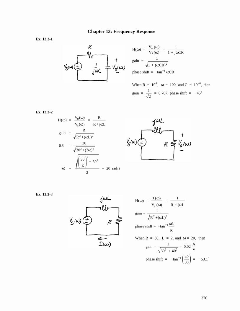
370

Chapter 13: Frequency Response

Ex. 13.3-1 Ex. 13.3-2 Ex. 13.3-3

H

phase shif

( )ω ωω ω

ω

ω

= V ( )

V ( ) =

11 + j CR

gain = 1

1 + ( CR)

t = tan CR

o

s

2

− −1

When R = 10 , = 100, and C = 10 , then

gain = 1

2 = 0.707, phase shift = 45

4 6

o

ω −

−

H

gain

( )( )

( )

.

ω ω

ω ω

ω

ω

ω

= V

V =

R

R+ j L

= R

R +( L)

= 30

30 +(2 )

=

30

.6 30

2 = 20 rad s

0

s

2 2

2 2

2

0 6

2

−

When R = 30, L = 2, and = 20, then

gain = 1

30 + 40 = 0.02

AV

phase shift = tan 4030

= 53.1

2 2

1

ω

−

−− °

H

gain

phase shif

( )ω ω

ω ω

ωω

= I ( )

V ( ) =

1

R + j L

= 1

R +( L)

t = tanL

R

s

2 2

1− −

371

Ex. 13.3-4 Ex. 13.3-5 Ex. 13.4-1

Ex. 13.4-2 Ex. 13.4-3

H

gain

phase shif

( )ω ωω ω

ω

ω

= V ( )

V ( ) =

11 + j CR

= 1

1 + ( CR)

t = tan CR

o

s

2

1− −

− − ⋅ ⋅ ⇒⋅

⋅° − −°

− 45 = tan (20 10 R =

tan (45

20 10= 50 10 1 6

6

3R)) Ω

H

gain

( )ω ωω ω

ω

= V ( )

V ( )=

11 + j CR

= 1

1 + ( CR)

o

s

2

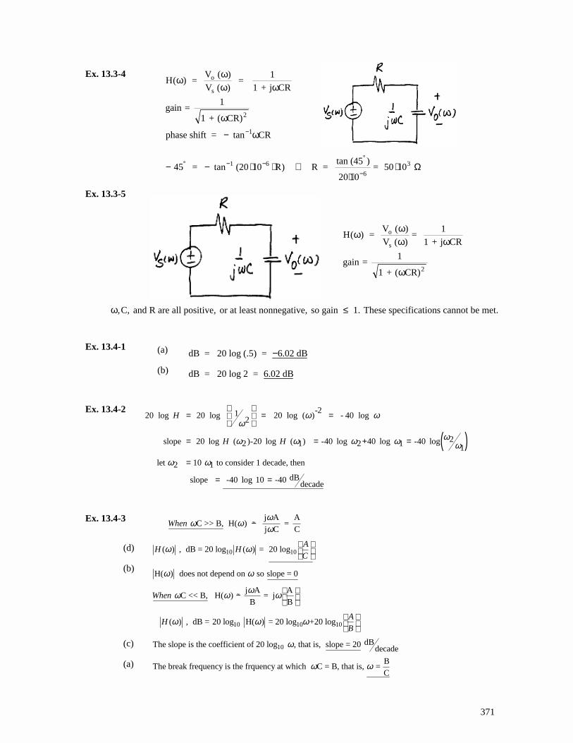
ω, ,C and R are all positive, or at least nonnegative, so gain 1. These specifications cannot be met.≤

dB = 20 log 2 = 6.02 dB

(a) dB = 20 log (.5) = 6.02 dB−

(b)

( )

-2120 log 20 log 20 log ( ) - 40 log 2

2slope 20 log ( )-20 log ( ) -40 log 40 log -40 log2 1 2 1 1

let 10 to consider 1 decade, then2 1

dBslope -40 log 10 -40 d

H

H H

ω ωω

ωω ω ω ω ω

ω ω

= = =

= = + =

=

= = ecade

10 10

10

j A A C >> B, H( ) =

j C C

( ) , dB = 20 log ( ) = 20 log

H( ) does not depend on so slope = 0

j A A C << B, H( ) = j

B B

( ) , dB = 20 log H( ) = 20 l

When

AH H

C

When

H

ωω ω

ω

ω ω

ω ω

ωω ω ω

ω ω

−

−

10 10

10

og +20 log

dBThe slope is the coefficient of 20 log , that is, slope = 20 decade

BThe break frequency is the frquency at which C = B, that is, =

C

A

Bω

ω

ω ω

(b)

(c)

(a)

(d)

372

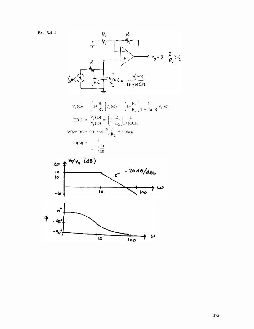
Ex. 13.4-4

V = 1+R

RV 1+

R

R1

1 + j CRV

= V

= 1+R

R1

1+ j CR

= 0.1 and R R = 3, then

H( ) = 4

1 + j10

1

2c

1

2s

o 1

2

1

2

o

s

HV

When RC

( ) ( ) ( )

( )( )

( )

ω ωω

ω

ω ωω ω

ω ω

=

373

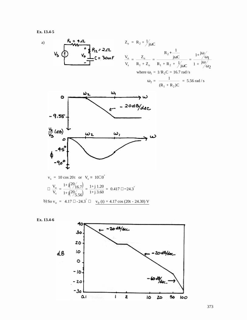
Ex. 13.4-5 Ex. 13.4-6

Z

V

V

j C

where

C

o

o

s

= R + 1j C

= Z

R + Z =

R

R + R + 1j C

= 1+ j

1

1 + j2

= 1/R C = 16.7 rad /s

= 1

(R + R = 5.56 rad / s

2

o

1 o

2

1 2

1 2

2

1 2

ω

ω

ω

ωω

ωω

ω

ω

+ 1

)

a)

b)

v

So v

s = 10 cos 20 t or V 10 0

V

V =

1+ j 2016.7

1+ j 205.56

= 1+ j 1.201+ j 3.60

= 0.417 24.3

= 4.17 - 24.3 v (t) = 4.17 cos (20t - 24.30) V

s

o

s

o 0

= ∠

∴ ∠−

∠ ⇒

°

°

°

374

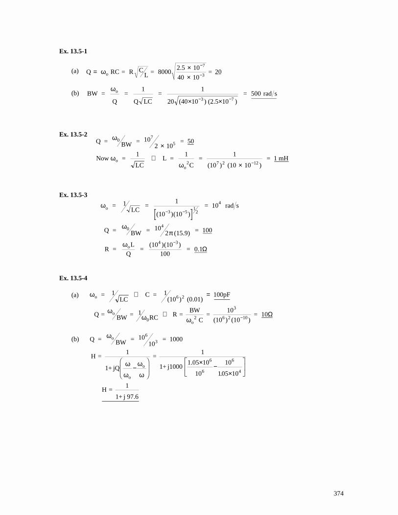
Ex. 13.5-1 Ex. 13.5-2 Ex. 13.5-3 Ex. 13.5-4

Q = ××

−

− RC = R CL = 8000

2.5 10

10 = 20o

7

3ω

40(a)

(b) BW = Q

= 1

Q LC =

1

20 (40 10 ) (2.5 10 = 500 rad so

3 7

ω

× ×− − )

Q BW

Now C

= = 10 10

= 50

= 1

LC L =

1 =

1

(10 (10 10 = 1 mH

07

5

o

o7 12

ω

ωω

2

2 2

×

⇒× −) )

ω

ωπ

ω

o3 5

4

04

o4 3

= 1LC

= 1

(10 (10 = 10 rad s

Q = = 10 (15.9) = 100

R = Q

= (10 (10

= 0.1

− −

−

) )

) )

12

2

100

BW

LΩ

ω

ωω ω

o 6

o

0 o

3

6 10

= 1LC

C = 1(10 (0.01)

100pF

= = 1 R = BW

C =

10

(10 (10 = 10

⇒ =

⇒ −

)

) )

2

2 2Q BW RC Ω

(a)

(b) Q = = 10 = 1000

H = 1

1+ jQ

= 1

1+ j1000 1.05 10 10

10

H = 1

1+ j 97.6

o6

6 6

4

ω

ω

ω

ω

ω

BW

o

o

10

10 105

3

6−

× −×

.

375

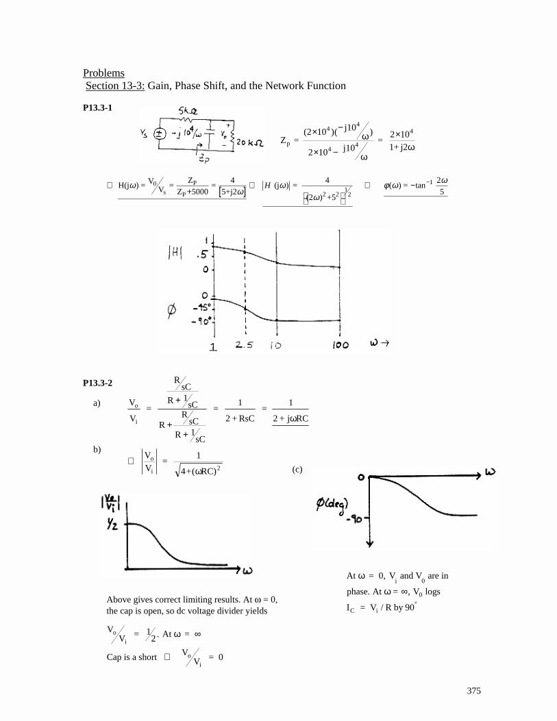
Problems Section 13-3: Gain, Phase Shift, and the Network Function P13.3-1 P13.3-2

[ ]1P0

1s 2 2P 2

Z 4 4 2V H(j ) = = = (j ) = ( ) = tan V Z 5000 5+j2 5(2 ) +5

Hωω ω φ ω

ωω

−∴ ⇒ ⇒ −+

Zp = (2 10 ( j10

10 j10 =

2 101+ j2

44

44

4× −

× −

×) )ω

ωω

2

a)

b) ⇒

V

V =

1

4+( RC)

o

i 2ω

VV = 1

2 At =

Cap is a short VV = 0

o

i

o

i

. ω ∞

⇒

Above gives correct limiting results. At = 0, the cap is open, so dc voltage divider yields

At are in

R by 90

ω

ω

= 0, V and V phase. At = V logs

I = V

i 0

0

C i

∞°

,

/

V

V

RsC

R sC

RR

sC

R sC

o

i

= = 1

2 + RsC =

1

2 + j RC

+

++

1

1

ω

(c)

376

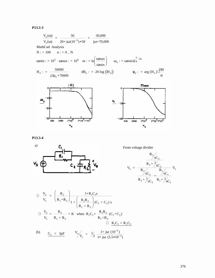
P13.3-3 P13.3-4

V

V

MathCad A

N :

H

o

s

n

( )

( ) )

ω

ω ω ω

ω ω ω

ωω ω

ωφ

π

= 50

20+ j (10 =

50,000

j +70,000

nalysis

= 100 n : = 0 .. N

min : = 10 max : = 10 m : = lnmax

min : = min e

: = 50000

j +70000dB : = 20 log H : = arg H

3

2 6n

n

N m

n

n n n n

−

⋅

+

⋅

⋅⋅

50

180

From voltage divider

V = + 1

sC

RsC

R + 1sC

+

RsC

R + 1sC

V2

2

2

22

1

1

11

so

RsC

R

2

2

2

⇒

∴

⇒

V

V =

R

R +R

1+R

+ R

+ R (C + C s

V

V =

R

R + R = K when R =

R

+R+C

R = R

o

s

2

1 2

1

1

2

1 2

o

s

2

1 2

11

2

2

1 2

C s

R

R

CR

RC

C C

1

2

1

12

1

1

1 2

1 )

( )

(b) C = 1 F1 µ VV = 1

2 1+ j (10 )

j (5.5 10 )o

s

ωω

−

−+ ×

2

31

a)

377

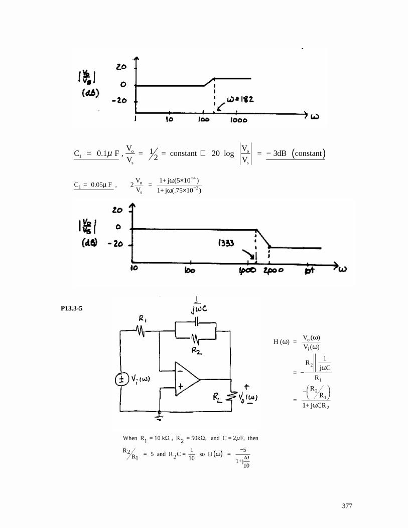
P13.3-5

( )o o1

s s

V V1C 0.1 F , = = constant 20 log = 3dB constant2V Vµ= ∴ −

C = 0.05 F , 2V

V =

1+ j (5 10 )

1+ j (.75 10 )1

o

s

µ ωω

××

−

−

4

3

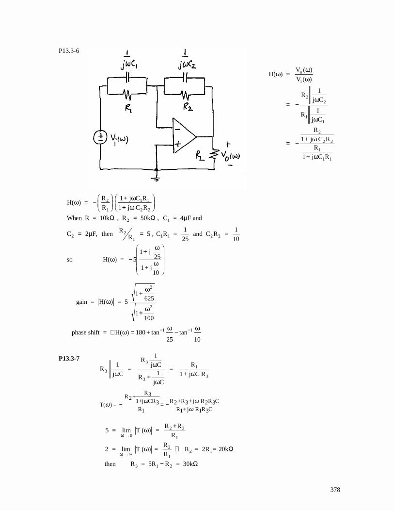
H ( ) = V

V ( )

=

R 1

j C

R

=

RR

1+ j CR

o

i

2

1

2

1

2

ω ωω

ω

ω

( )

−

−

( )

When R = 10 k , R = 50k , and C = 2 F, then1 2

1 5R2 5 and R C = so H R 21 10 1+j10

µ

ω ω

Ω Ω

−= =

378

P13.3-6 P13.3-7

gain = H( ) = 5 1+

2

ω

ω

ω625

1100

2

+

phase shift = H( )∠ = + −− −ω ω ω180

25 10

1 1tan tan

H( ) V

V

Rj C

Rj C

R

1+ j C RR

1+ j C R

o

i

22

11

2

2 2

1

1 1

ωωω

ω

ω

ω

ω

=

= −

= −

( )

( )

1

1

C F, then RR C R =

1

25 and C R =

1

10

so H( ) = j

25

1+ j10

22

11 1 2 2= =

−+

2 5

51

µ

ω

ω

ω

,

H( ) = R

R

1+ j C R

j C R

When R = 10k , R k , C = 4 F and

2

1

1 1

2 2

2 1

ωωω

µ

−

+

=1

50Ω Ω

R 1

j C =

Rj C

Rj C

= R

1+ j C R3

3

3

1

3ωω

ωω

1

1+

R3 R2 1+j CR R +R j R R C3 2 3 2 3T( ) = R R j R R C1 1 1 3

ω ωωω

++− = −

+

5 T ( ) = R R

R

2 = T ( ) = R

R R = 2R = 20k

then R = 5R R = 30k

0

2 3

1

2

12 1

3 1 2

= +

⇒

−

→

→∞

lim

lim

ω

ω

ω

ω Ω

Ω

379

P13.3-8 P13.3-9 P13.3-10

T ( ) = R

j

R =

j CR

j CR

T( ) = 180 + tan CR

T( ) = 135 tan CR = 45

CR

R = 1

10 = 10k

10 = T( ) = R

R R

R

10 k

2

1

2

1

2

2

2

2 3

2

11

2

ω ω ωω

ω ω

ω ωω

ωω

−+

−+

∠ −

∠ ⇒⇒ =

⇒

⇒ = =

−

−

−

→∞

11

90

1

10

1

1

1

7

C

Ω

Ωlim

( ) R j CR2 2T = 1 1+j CR1+j C

R2 10 lim T( ) R 10R2 1R1

1 T( ) = 180+90 tan CR1

tan (270 T( )) 4 4 R = = 10 tan (270 T( )) = 10 = 10 k1 C

R = 100k2

ωω

ωω

ωω

ω ω

ω ωω

−= −

= = ⇒ =→∞

−∠ −

−∠⇒ ⋅ −∠ Ω

⇒ Ω

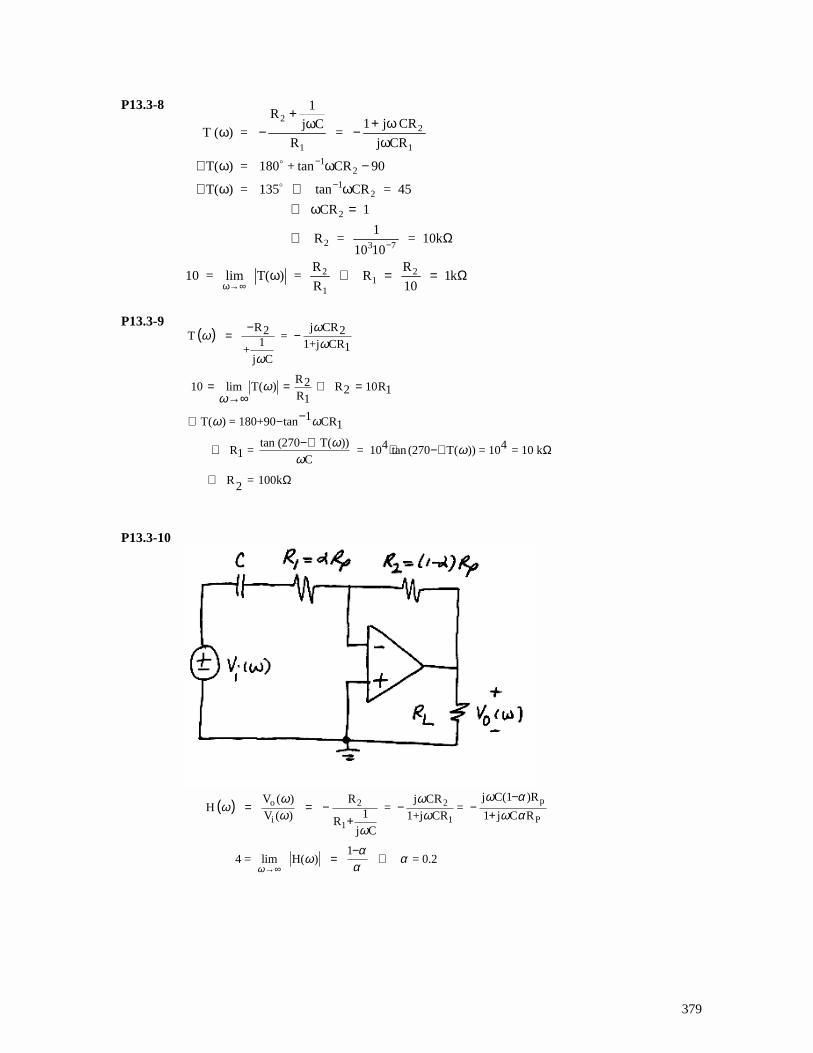
( ) po 2 2

i 1 P1

j C(1 )RV ( ) R j CRH = = 1V ( ) 1+j CR 1 j C RR

j C

14 = lim H( ) = 0.2

ω

ω αω ωω

ω ω ω αωα

ω αα→∞

−= = − − −

++

−= ⇒

380

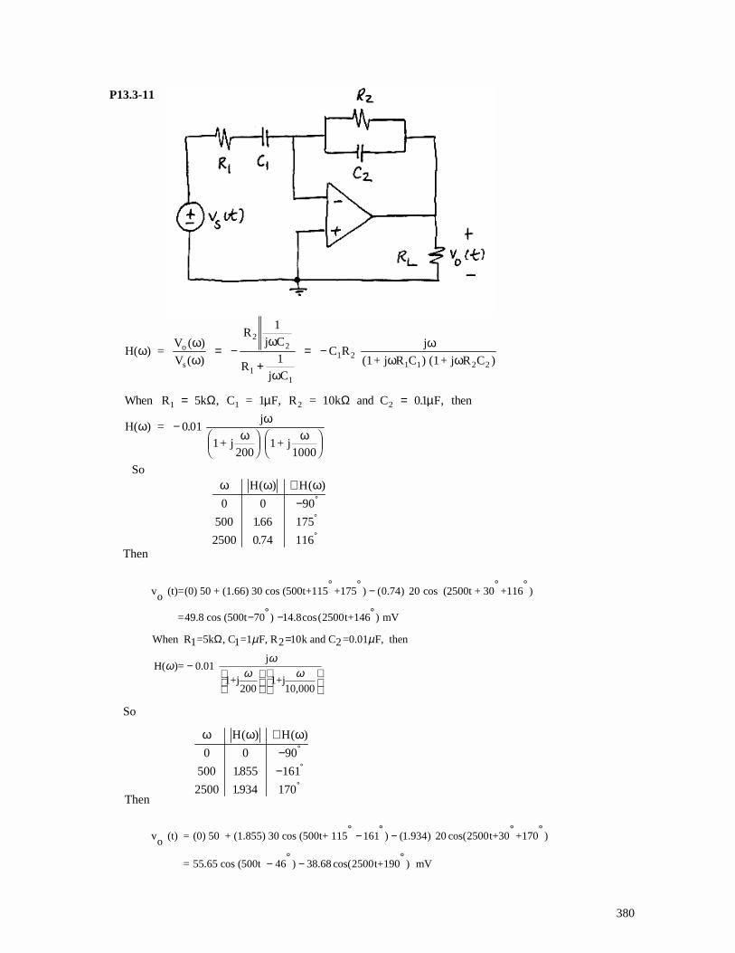
P13.3-11

H( ) = V

V

Rj C

Rj C

C R j

(1+ j R C ) (1+ j R C )o

s

22

11

1 21 1 2 2

ωωω

ω

ω

ωω ω

( )

( )= −

+= −

1

1

When R k , C = 1 F, R = 10k and C F, then

H( ) = j

1+ j200

1+ j1000

1 1 2 2= =

−

5 01

0 01

Ω Ωµ µ

ω ωω ω

.

.

So

Then

v (t)=(0) 50 + (1.66) 30 cos (500t+115 +175 ) (0.74) 20 cos (2500t + 30 +116 )o

=49.8 cos (500t 70 ) 14.8cos(2500t+146 ) mV

When R =5k , C =1 F, R 10k and C =0.01 F, then1 1 2 2

jH( )= 0.01

1+j 200

µ µ

ωω

ω

° ° ° °−

° °− −

Ω =

−

1+j10,000

ω

So

Then

v (t) = (0) 50 + (1.855) 30 cos (500t+ 115 161 ) (1.934) 20 cos(2500t+30 +170 )o

= 55.65 cos (500t 46 ) 38.68 cos(2500t+190 ) mV

° ° ° °− −

° °− −

ω ω ωH H( ) ( )

.

.

∠− °

°

°

0 0 90

500 166 175

2500 0 74 116

ω ω ωH H( ) ( )

.

.

∠−−

°

°

°

0 0 90

500 1855 161

2500 1934 170

381

P13.3-12

a) V =(8 div)

2 Vdiv

= 8 V

V =(6.2div)

2Vdiv

2= 6.2 V

gain =V

V=

6.2

8

s

o

o

s

=

2

0 775.

b)

H( ) =V

V =

1j C

R +1

j Cj CR

H( )C R

Let g = H( ) =1

1+ C RThen

C =1

R

1

g

o

s

2

2 2 2

2

ωωω

ω

ωω

ωω

ωω

ω

( )

( )=

+

=+

−

1

1

1

1

1

2 2

∠ −

= −∠

− H( ) = RC

so

tan( H( ))RC

ω ω

ω ω

tan 1c)

Recalling that R = 1000 and C=0.26µF, we calculate ω ω ωππ

H( ) H( )

2 (200) 0.95

0.26

∠−−

°

°18

2 2000 73( )

( )( ) ( )

tan 45Next , H( )= 45 requires = 3846 rad

61000 .2610

tan ( ( 135))Similarly , H( ) 135 requires = = 3846 rad s6(1000) (0.2610 )

sω ω

ω ω

° − − ° ∠ − =−⋅

− −°∠ = − −−⋅

A negative frequency is not acceptable. We conclude that this circuit cannot produce a phase shift equal to −135°.

In this case = 2 500 = 3142 rad s, ( ) 0.775 and R=1000 so C = 0.26 F.Hω π ω µ⋅ = Ω

382

Section 13-4: Bode Plots P13.4-1

H( ) =20 1+ j

5

1+ j50

ω

ω

ω

d) C = tan ( H( ))

R

C = tan ( ))

(2 500) (1000) = 0.55 F

C = tan ( )

(2 500 ) (1000) = 0.55 F

−∠

−

⋅

− −

⋅−

°

°

ω

ω

πµ

πµ

(

( )

60

300

A negative value of capacitance is not acceptable and indicates that this circuit cannot be designed to produce a phase shift at −300° at a frequency of 500 Hz.

e) C = tan( )

F− −⋅

= −°( )

( )( ).

120

2 500 1000 55

πµ

This circuit cannot be designed to produce a phase shift of −120° at 500 Hz.

H( )ω ~−

20 < 5

20 j5

= j4 5 < < 50

20

j5

j50

= 200 50 <

ω

ω ω ω

ω

ω ω

383

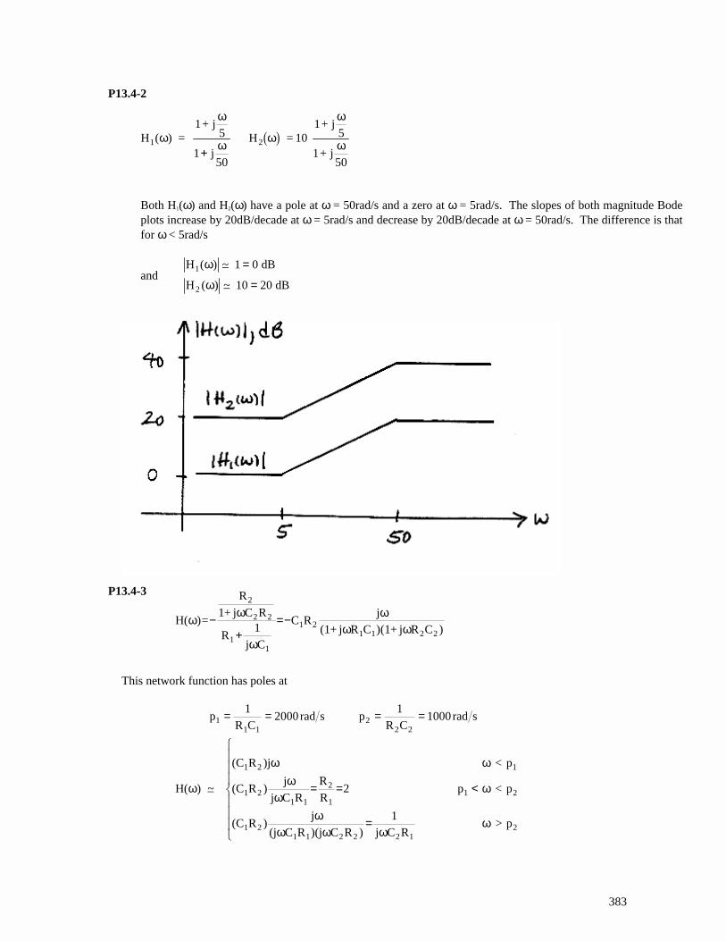
P13.4-2 P13.4-3

H ( ) = 1+ j

j50

H = 10 1+ j

5

1+ j50

1 2ω

ω

ω ω

ω

ω5

1+

Both H1(ω) and H2(ω) have a pole at ω = 50rad/s and a zero at ω = 5rad/s. The slopes of both magnitude Bodeplots increase by 20dB/decade at ω = 5rad/s and decrease by 20dB/decade at ω = 50rad/s. The difference is thatfor ω < 5rad/s

H dB

H dB

1

2

( ) ~_

( ) ~_

ω

ω

1 0

10 20

=

=

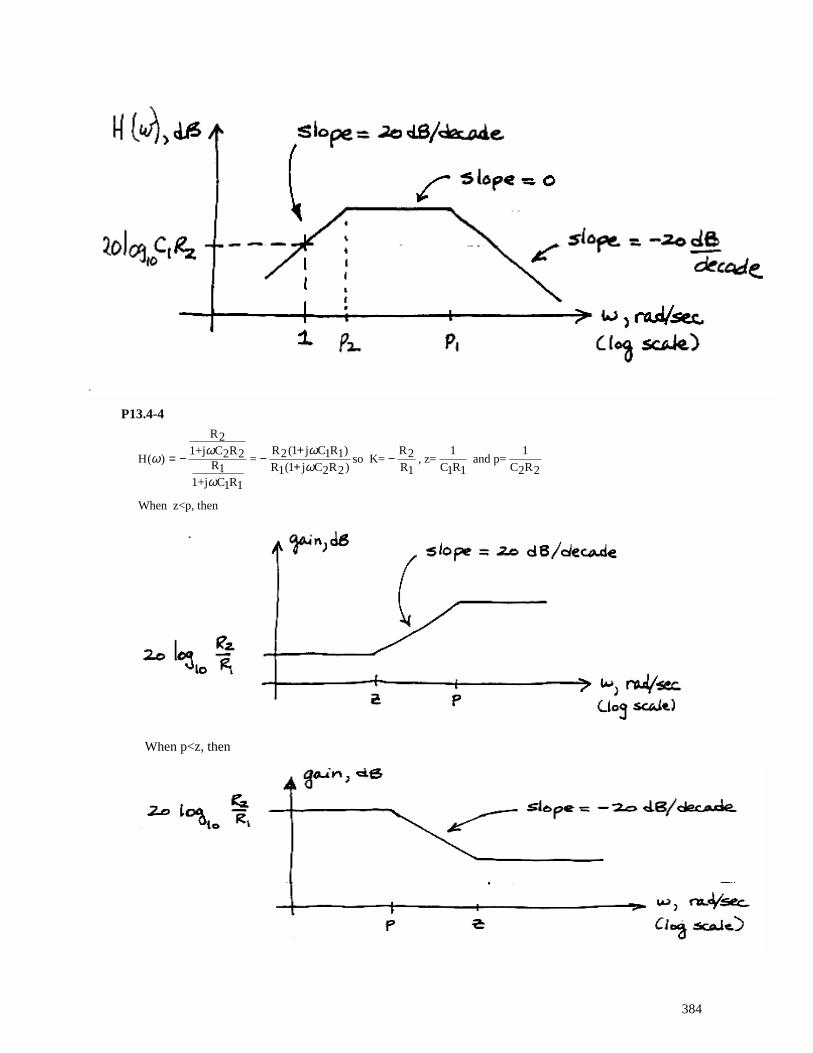
H( )=

R

1+ j C R

Rj C

C Rj

(1+ j R C )(1+ j R C )

2

2 2

11

1 21 1 2 2

ω ω

ω

ωω ω

−+

=−1

This network function has poles at

pR C

s pR C

H( )

(C R )j < p

(C R )j

j C R

R

Rp < p

(C R )j

(j C R )(j C R ) j C R > p

11 1

22 2

1 2 1

1 21 1

2

11 2

1 21 1 2 2 2 1

2

= = = =

= = <

=

12000

11000

2

1

rad rad s

ω

ω ωω

ωω

ωω ω ω

ω

~_

and

384

P13.4-4

R2R (1 j C R ) R 1 11+j C R 2 1 1 22 2H( ) = so K= , z= and p=R R (1 j C R ) R C R C R1 1 2 2 1 1 1 2 2

1+j C R1 1

When z<p, then

ωωω

ωω

+= − − −

+

When p<z, then

385

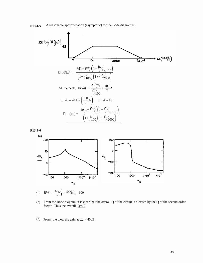
P13.4-5 P13.4-6

A reasonable approximation (asymptotic) for the Bode diagram is:

∴ ×

+

∴

⇒

⇒

×

H(j ) = A 1+ j 7 1+ j

3 10j100 1+ j

2000

At the peak, H(jA j

7j

100

=100

7A

43 = 20 log 100

7A A = 10

H(j ) = 10 1+ j

7 1+ j3 10

1+ j100 1+ j

2000

4

4

ωω ω

ω

ωω

ω

ω

ω ω

ω

1

) ~_

(a)

(b) BW = Qω0 1000

10 100= =

(c) From the Bode diagram, it is clear that the overall Q of the circuit is dictated by the Q of the second order factor. Thus the overall Q=10

(d) From, the plot, the gain at = 40dBω0

386

P13.4-7 P13.4-8

By inspection,

H(j ) = A 1+ j 100

j 1+ j 1000from the magnitude plot for 100< <1000

H(j ) Aj 100j

A100

20log A100=0 A=100

So H(j ) = 100 1+ j 100

j 1+ j 1000

ωω

ω ω

ω

ωω

ω

ωω

ω ω

~− =

∴ ⇒

1 20 71

2

+ −

δ ω ω

j0.7 .

1 2

1 20 7

1 2600

1

0

0 7

2

2

1

2

2

2

2

+ −

+ −

+ −

+

=

−

= ⇒

δ ω ω

ω

ω ω

δ ω ω δ ω ω ω

ω ω

ω

ω

j600 600

H( ) =

K(1+ j10

)(j )

j0.7

j600

j100

To determine K, notice that H dB=1 when 0.7 < < 10. That is

1 =K(1)(j )

(1)(1)

K(0.7) K = 2

2

22

.

.

• The slope is 40dB/decade for low frequencies, so the numerator will include the factor (jω)2 . • The slope decreases by 40dB/decade at ω = 0.7rad/sec. So there is a second order pole at ω0 = 0.7rad/sec. The

damping factor of this pole cannot be determined from the asymptotic Bode plot; call it δ1. The denominator of the network function will contain the factor

• The slope increases by 20dB/decade at ω = 10rad/s, indicating a zero at 10rad/s. • The slope decreases by 20dB/decade at ω = 100rad/s, indicating a pole at 100rad/s. • The slope decreases by 40dB/decade at ω = 600rad/s, indicating a second order pole at ω0 = 600rad/s. The

damping factor of this pole cannot be determined from an asymptotic Bode plot; call it δ2. The denominator of the network function will contain the factor

387

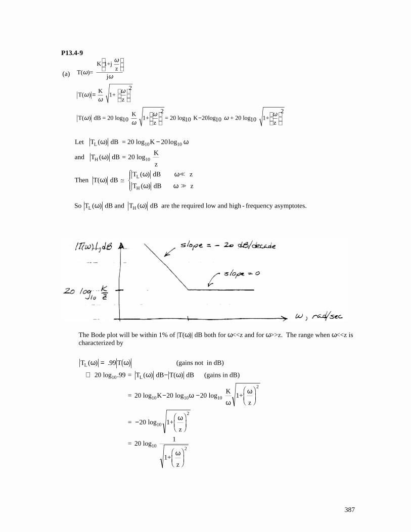
P13.4-9

T ( ) T (gains not in dB)

20 log .99 = T ( ) dB T( ) dB (gains in dB)

= 20 log K log log K

1+z

= log 1+z

= 20 log 1

1+z

L

10 L

10

2

2

102

ω ω

ω ω

ωω

ω

ω

ω

=

⇒ −

− −

−

.99

20 20

20

10 10

10

(a)

K 1+j z

T( )= j

2KT( ) 1+

z

2 2KT( ) dB = 20 log 1+ = 20 log K 20log + 20 log 1+10 10 10 10z z

ω

ωω

ωωω

ω ωω ωω

=

−

So T ( ) dB and T ( ) dB are the required low and high - frequency asymptotes.L Hω ω

The Bode plot will be within 1% of |T(ω)| dB both for ω<<z and for ω>>z. The range when ω<<z is characterized by

Let T ( ) dB = 20 log K

and T dB = 20 log K

z

Then T( ) dB T ( ) dB << z

T dB >> z

L 10

H 10

L

H

ω ω

ω

ωω ω

ω ω

−

20 10log

( )

~_( )

388

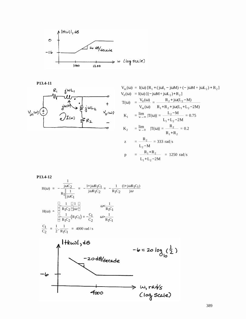
P13.4-10

The range when acterized by

T T( ) (gains not in dB)

20 log .99 = T dB T( ) dB (gains in dB)

= 20 log K log z logK

1+z

= logz

1+z

= 20 log101

Z2

+1

H

10 H

10

2

2

ωω ω

ω ω

ω

ω

ω

ω

ω

>>=

⇒ −

− −

−

z is char

( ) .

( )

99

20 20

20

10 10

10

z

= .99

= z

1

.99

= z

.147z

The error is less than 1% when <z

7 and when > 7z.

2

2

⇒

−

⇒

−

−

ω

ω

ω ω

11

1

~

H V

V

R

R RjwC

R

RR

jwCR

H R j

R R j CR R

R

R R

j

jCR R

R +R

s

t

t

t

t

t

t t

t

t

t

( )( )

( )

( )( )

ω ωω

ω ωω

ω

ω

= =+

=+

+

= ++ +

=+

+

+

0

11

1

1

1 1 1

1

1

1

11

1 1

1

CR CR

t

When R 1k , C 1 F and R 5k1 t

5 1000

61 j5 51000H( ) H( ) j 1000 1200

6 6 10001 j1200 1 1200

µ

ωω

ωω ω ωωω

= Ω = = Ω

< + = ⇒ ≅ < < + <

⇒

⇒

− − .99 = 1

1+z

= z.99

= .14z z

72

2

ωω 1

1 ~

389

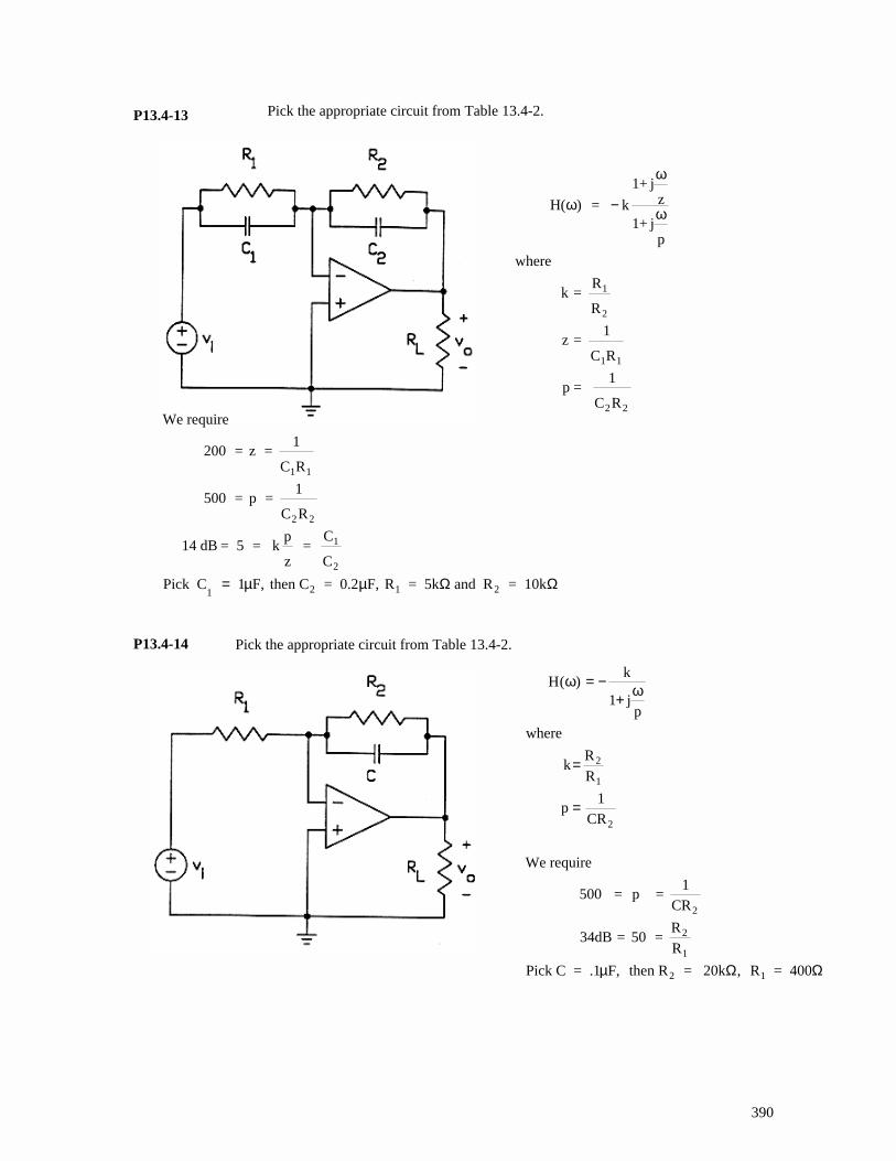
P13.4-11 P13.4-12

( )

11 j R C 1 (1 j R C )j C 1 1 1 12H( )

j R C R C j1 1 2 1 2R1 j C1

1 1 1

R C j R C1 2 1 1H( ) 1 C 11R C 1 1R C C R C1 2 2 1 1

C 1 11 , 4000 rad / sC 2 R C2 1 1

ω ωωω

ω ωω

ωω

ωω

+ += − = − = −

− < − − = − >

= =

V ) = I( ) [R j l j M) + ( j M + j L R

V ) = I( ) [( j M+ j L R

T( ) = V )

V ) =

R j (L M)

R R j (L L M)

K = lim |T( )| = L M

L +L M = 0.75

K = lim T( =

R

R R = 0.2

z = R

L M = 333 rad s

p

in 1 1 2 2

0 2 2

0

in

2 2

1 2 1 2

1 w2

1 2

2 w 02

1 2

2

2

( ( ) ]

( ) ]

(

(

| )|

ω ω ω ω ω ωω ω ω ω

ω ω

ω

ω

ω

ω

ω

+ − − +− +

+ −

+ + + −−

−

+

−

→∞

→

2

2

= R R

L L M = 1250 rad s1 2

1 2

+

+ −2

390

P13.4-13 P13.4-14

Hk

jp

where

kR

R

pCR

( )ω ω= −+

=

=

1

1

2

1

2

We require

200 = z = 1

C R

500 = p = 1

C R

14 dB = 5 = kp

z =

C

C

1 1

2 2

1

2

Pick C 1 F, then C = 0.2 F, R = 5k and R = 10k1 2 1 2= µ µ Ω Ω

H( ) = k

1+ jz

1+ jp

where

k = R

R

z = 1

C R

p = 1

C R

1

2

1 1

2 2

ω

ω

ω−

We require

500 = p = 1

CR

34dB = 50 = R

R

Pick C = .1 F, then R = 20k , R = 400

2

2

1

2 1µ Ω Ω

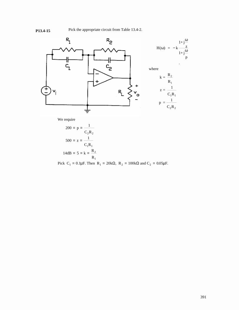
Pick the appropriate circuit from Table 13.4-2.

Pick the appropriate circuit from Table 13.4-2.

391

P13.4-15

H

where

R

p R

( )ω

ω

ω = k

1+ jz

1+ jp

.

k = R

R

z = 1

C

=1

C

2

1

1

2

−

1

2

We require

p

z

14 k R

R

0.1 Then R R 100 and C

2

1

2001

5001

5

20 0 05

2 2

1 1

1 1 2 2

= =

= =

= = =

= = = =

C R

C R

dB

Pick C F k k Fµ µ. , . .Ω Ω

Pick the appropriate circuit from Table 13.4-2.