Control systems - Frequency domain analysis: Polar Plot
23
Outline Control systems Frequency domain analysis: Polar Plot V. Sankaranarayanan V. Sankaranarayanan Frequency domain analysis
Transcript of Control systems - Frequency domain analysis: Polar Plot

Outline
Control systemsFrequency domain analysis: Polar Plot
V. Sankaranarayanan
V. Sankaranarayanan Frequency domain analysis

Outline
Outline
V. Sankaranarayanan Frequency domain analysis

Polar plot
It is a plot of the magnitude of G(jω) versus the phase angle of G(jω) onpolar coordinates as ω is varied from zero to infinity
In polar plots a positive (negative) phase angle is measured counterclockwise(clockwise) from the positive real axis
V. Sankaranarayanan Frequency domain analysis
Integral and derivative factors
Integral and derivative factors
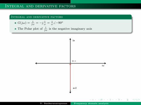
G(jω) = 1jω
= −j 1ω
= 1ω∠−90o
The Polar plot of 1jω
is the negative imaginary axis
V. Sankaranarayanan Frequency domain analysis

Integral and derivative factors
Integral and derivative factors
The Polar plot of jω is the positive imaginary axis
V. Sankaranarayanan Frequency domain analysis

First order factors
First order factors
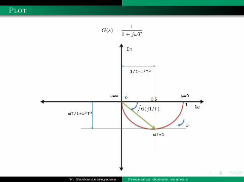
G(jω) = 11+jωT
= 1√1+ω2T2
∠−tan−1ωT
G(j0) = 1∠0o, G(j 1T
) = 1√2∠45o
ω −→∞, |G(jω)| −→ 0 and ∠G(jω) −→ −90o
G(s) = X + jY
1
1 + jωT=
1− jωT1 + ω2T 2
G(s) =1
1 + ω2T 2− j
wT
1 + ω2T 2
X =1
1 + ω2T 2Y = −
wT
1 + ω2T 2(X −
1
2
)2
+ Y 2 =
(1
2
)2
So the polar plot is a semi circle.
V. Sankaranarayanan Frequency domain analysis
Plot
G(s) =1
1 + jωT
V. Sankaranarayanan Frequency domain analysis

First order factors
First order factors
G(jω) = 1 + jωT
It is simply the upper half of the straight line passing through point (1, 0) inthe complex plane and parallel to the imaginary axis
V. Sankaranarayanan Frequency domain analysis

Quadratic factors
Quadratic factors
G(jω) = 11+2ζ(j ω
ωn)+(j ω
ωn)2
For ζ > 0
limω→0
G(jω) = 1∠0
limω→∞
G(jω) = 0∠−180
The polar plot of this sinusoidal transfer function starts at 1∠0 and ends at0∠−180 as ω increases from zero to infinity
The high-frequency portion of G(jω) is tangent to the negative real axis.
For the underdamped case ω = ωn, the phase angle is −90
In the polar plot, the frequency point whose distance from the origin ismaximum corresponds to the resonant frequency ωr.
V. Sankaranarayanan Frequency domain analysis

V. Sankaranarayanan Frequency domain analysis

Quadratic factors
Quadratic factors
G(jω) = 1 + 2ζ(j ωωn
) + (j ωωn
)2
=(
1− ω2
ω2n
)+ j
(2ζωωn
)limω→0
G(jω) = 1∠0
limω→∞
G(jω) =∞∠180
V. Sankaranarayanan Frequency domain analysis

V. Sankaranarayanan Frequency domain analysis
Gain Margin and Phase Margin
Gain Margin
The gain margin is the reciprocal of the magnitude |G(jω)| at the frequency atwhich the phase angle is −180o(Phased cross over frequency)
Kg =1
|G(jω)|at∠G = −180o
Phase Margin
The phase margin is the amount of additional phase lag at the gain cross overfrequency required to the verge of instability γ = 180o + φ
V. Sankaranarayanan Frequency domain analysis

Phase and Gain Margin
Nyquist Diagram
Real Axis
Imagin
ary
Axis
−1 −0.8 −0.6 −0.4 −0.2 0 0.2 0.4 0.6 0.8 1−1
−0.8
−0.6
−0.4
−0.2
0
0.2
0.4
0.6
0.8
1
Phase Cross Over at (−0.5,0)
Gain Margin=2
Unit Circle
Gain Cross Over
Phase Margin=44.1
V. Sankaranarayanan Frequency domain analysis
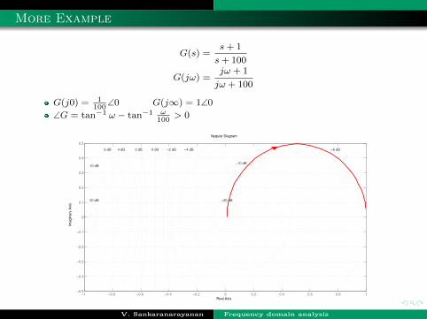
More Example
G(s) =s+ 1
s+ 100
G(jω) =jω + 1
jω + 100
G(j0) = 1100
∠0 G(j∞) = 1∠0
∠G = tan−1 ω − tan−1 ω100
> 0
Nyquist Diagram
Real Axis
Imagin
ary
Axis
−1 −0.8 −0.6 −0.4 −0.2 0 0.2 0.4 0.6 0.8 1−0.5
−0.4
−0.3
−0.2
−0.1
0
0.1
0.2
0.3
0.4
0.5
0 dB
−20 dB
−10 dB
−6 dB−4 dB−2 dB
20 dB
10 dB
6 dB 4 dB 2 dB
V. Sankaranarayanan Frequency domain analysis
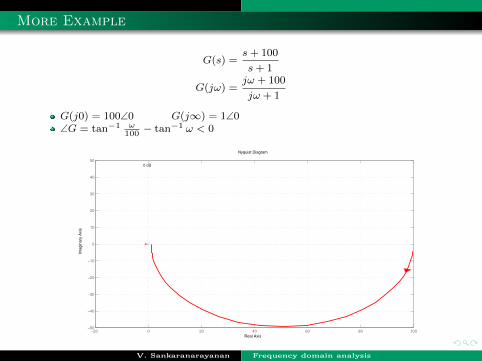
More Example
G(s) =s+ 100
s+ 1
G(jω) =jω + 100
jω + 1
G(j0) = 100∠0 G(j∞) = 1∠0∠G = tan−1 ω
100− tan−1 ω < 0
Nyquist Diagram
Real Axis
Imagin
ary
Axis
−20 0 20 40 60 80 100−50
−40
−30
−20
−10
0
10
20
30
40
50
0 dB
V. Sankaranarayanan Frequency domain analysis

Examples
G(s) =s+ 5
(s+ 1)(s+ 10)
G(j0) = 0.5∠0 G(j∞) = 0∠− 90o
−0.5 −0.4 −0.3 −0.2 −0.1 0 0.1 0.2 0.3 0.4 0.5−0.25
−0.2
−0.15
−0.1
−0.05
0
0.05
0.1
0.15
0.2
0.25
0 dB
−20 dB
−10 dB−6 dB−4 dB−2 dB
Nyquist Diagram
Real Axis
Imagin
ary
Axis
V. Sankaranarayanan Frequency domain analysis

Example
G(s) =1
s(sT + 1)
G(jω) =1
jω(jωT + 1)= −
T
1 + ω2T 2− j
1
ω(1 + ω2T 2)
limω→0
G(jω) = −T − j∞ =∞∠− 90o
limω→∞
G(jω) = 0− j0 = 0∠− 180o
Suppose G(s) =1
s(5s+ 1)
−2.5 −2 −1.5 −1 −0.5 0−80
−60
−40
−20
0
20
40
0 dB
−2 dB2 dB
Nyquist Diagram
Real Axis
Imagin
ary
Axis
V. Sankaranarayanan Frequency domain analysis
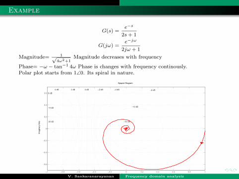
Example
G(s) =e−s
2s+ 1
G(jω) =e−jω
2jω + 1
Magnitude= 1√4ω2+1
Magnitude decreases with frequency
Phase= −ω − tan−1 4ω Phase is changes with frequency continously.Polar plot starts from 1∠0. Its spiral in nature.
−1 −0.8 −0.6 −0.4 −0.2 0 0.2 0.4 0.6 0.8 1
−0.6
−0.4
−0.2
0
0.2
0.4
0.6
0 dB
−20 dB
−10 dB
−6 dB−4 dB−2 dB
20 dB
10 dB
6 dB
4 dB 2 dB
Nyquist Diagram
Real Axis
Imagin
ary
Axis
V. Sankaranarayanan Frequency domain analysis

More Example
G(s) =s+ 10
(s+ 1)(s2 + 600s+ 1000000)
G(j0) = 10−5∠0 G(j∞) = 0∠− 180o
−1 −0.8 −0.6 −0.4 −0.2 0 0.2 0.4 0.6 0.8 1
x 10−5
−5
−4
−3
−2
−1
0
1
2
3
4
5x 10
−6Nyquist Diagram
Real Axis
Imagin
ary
Axis
V. Sankaranarayanan Frequency domain analysis

System Type and Polar Plot
G(s) =(s+ z1)(s+ z2) . . . . . . (s+ zm)
sk(s+ p1)(s+ p2) . . . . . . (s+ pn)n > m
Type 0 System:Starting point(ω = 0) isfinite and on real axis.Ending point(ω =∞) isat the origin.
−1 −0.5 0 0.5 1 1.5
−1
−0.5
0
0.5
1
0 dB
−20 dB
−10 dB
−6 dB
−4 dB−2 dB
20 dB
10 dB
6 dB
4 dB
2 dB
Nyquist Diagram
Real Axis
Imagin
ary
Axis
V. Sankaranarayanan Frequency domain analysis

System Type and Polar Plot
G(s) =(s+ z1)(s+ z2) . . . . . . (s+ zm)
sk(s+ p1)(s+ p2) . . . . . . (s+ pn)n > m
Type 1 System: Atω = 0 the magnitude is0 and phase become−90o.At low frequencypolar plot isasympototic to a lineparallel to imaginaryaxis. At ω =∞magnitude become zero.
−0.1 −0.05 0 0.05 0.1−8
−6
−4
−2
0
2
4
−10 dB−6 dB−4 dB
−2 dB
Nyquist Diagram
Real Axis
Imagin
ary
Axis
V. Sankaranarayanan Frequency domain analysis
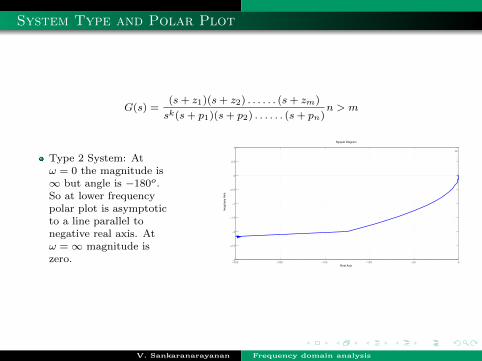
System Type and Polar Plot
G(s) =(s+ z1)(s+ z2) . . . . . . (s+ zm)
sk(s+ p1)(s+ p2) . . . . . . (s+ pn)n > m
Type 2 System: Atω = 0 the magnitude is∞ but angle is −180o.So at lower frequencypolar plot is asymptoticto a line parallel tonegative real axis. Atω =∞ magnitude iszero. −250 −200 −150 −100 −50 0
−3
−2.5
−2
−1.5
−1
−0.5
0
0.5
10 dB
Nyquist Diagram
Real Axis
Imagin
ary
Axis
V. Sankaranarayanan Frequency domain analysis


![1 Convolutional Polar Codes - arXiv · 1 Convolutional Polar Codes Andrew James Ferris, Christoph Hirche and David Poulin Abstract Arikan’s Polar codes [1] attracted much attention](https://static.fdocument.org/doc/165x107/5f07505c7e708231d41c5eb5/1-convolutional-polar-codes-arxiv-1-convolutional-polar-codes-andrew-james-ferris.jpg)