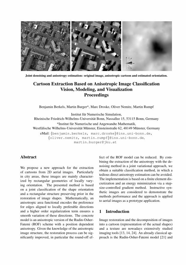
−π4

π4

Joint denoising and anisotropy estimation: original image, anisotropic cartoon and estimated orientation.

Cartoon Extraction Based on Anisotropic Image ClassificationVision, Modeling, and Visualization

Proceedings

Benjamin Berkels, Martin Burger*, Marc Droske, Oliver Nemitz, Martin Rumpf

Institut fur Numerische Simulation,Rheinische Friedrich-Wilhelms-Universitat Bonn, Nussallee 15, 53115 Bonn, Germany

*Institut fur Numerische und Angewandte Mathematik,Westfalische Wilhelms-Universitat Munster, Einsteinstraße 62, 48149 Munster, Germany

eMail: benjamin.berkels, marc.droske@ins.uni-bonn.de,oliver.nemitz, martin.rumpf@ins.uni-bonn.de,

martin.burger@jku.at

Abstract

We propose a new approach for the extractionof cartoons from 2D aerial images. Particularlyin city areas, these images are mainly character-ized by rectangular geometries of locally vary-ing orientation. The presented method is basedon a joint classification of the shape orientationand a rectangular structure preserving prior in therestoration of image shapes. Mathematically, ananisotropic area functional encodes the preferencefor edges aligned to locally preferable directionsand a higher order regularization term ensures asmooth variation of these directions. The concretemodel is an anisotropic version of the Rudin-Osher-Fatemi (ROF) scheme with a position dependentanisotropy. Given the knowledge of the anisotropicimage structure, the restoration process can be sig-nificantly improved, in particular the round-off ef-

fect of the ROF model can be reduced. By com-bining the extraction of the anisotropy with the de-noising method in a joint variational approach, weobtain a suitable classification method, in which atedious direct anisotropy estimation can be avoided.The implementation is based on a finite element dis-cretization and an energy minimization via a step-size-controlled gradient method. Instructive syn-thetic images are considered to demonstrate themethods performance and the approach is appliedto aerial images as a prototype application.

1 Introduction

Image restoration and the decomposition of imagesinto a cartoon (representation of the actual shapes)and a texture are nowadays extensively studiedimaging tools [13, 14, 24]. An already classical ap-proach is the Rudin-Osher-Fatemi model [21] and

variants of this method [15, 7, 28]. These meth-ods are well-suitable to restore sharp edge con-tours. But at corners formed by edges they comealong with a significant rounding artifact. In partic-ular for images characterized by rectangular shapesthis hampers the identification of structures and de-stroys a proper cartoon representation. Conceptsfor anisotropic variational approaches, such as thosepresented in [9, 18], and the anisotropic variantof the Rudin-Osher-Fatemi model by Esedoglu andOsher [12] point out a suitable modification, whichwe are developing further here. As a prototype ap-plication we consider aerial images of city zones,the technique is however also suitable for othertypes of images with similar morphologies. Hence,we obtain the following problem set-up: We as-sume, that the given possibly noisy and locally de-stroyed image contains primarily structures withstraight edges and corners with right angles. Fur-thermore, we assume that the orientation of thesestructures varies in space. In particular we do notfix an orientation a priori. The aim is now to extracta cartoon representation of image shapes, while pre-serving or even enhancing edges and sharp corners.This extraction can also be regarded as an imagerestoration technique.

Let us briefly review the state of the art. There al-ready exists a large variety of approaches to featurepreserving image restoration, as for example non-linear diffusion methods [26] (see also Fig. 6) andthe Rudin-Osher-Fatemi (ROF) model. The ROF-model is the fundamental basis for a wide range ofimage decomposition models, which separate theinput signal into a cartoon part u and a texturepart v (c. f. for instance [2, 3]). Inspired by Y.Meyer’s idea [17] to characterize textures by func-tions with a bounded ‖·‖∗ norm, i. e., the dual normof the BV -norm, the key ingredient for decomposi-tion problems is the study of qualitative propertiesfor different norms in which the fidelity u − u0 ismeasured.

Several methods were introduced to approximatethis problem by related problems, that are com-putationally feasible and yield qualitatively similarresults [20, 13]. Recently, decomposition modelsbased on a L1-fidelity have attracted much attentiondue to their desirable scale decomposition proper-ties [15, 7, 28].

It is well known, that the restored image of theROF-model often suffers from a significant loss of

contrast. An iterative procedure based on Breg-man iterations leads to a sequence of decreasingscale, converging back to the original image, wherethe loss of contrast is compensated already in veryearly stages of the iteration [23, 19, 6, 5]. In thecontinuous setting, this process can be interpretedas an inverse scale space. The focus of this pa-per is the study of the classical ROF model withan anisotropic BV -norm. Based on the theory ofanisotropically aligned microstructures [27, 1, 25],the concept of so-called Wulff shapes has been usedto denoise surfaces [9] and images [12] using es-timated a-priori information about the shape ofthe object to be denoised. In [18] the anisotropicstructure of blood vessels has been determined ina first estimation step and subsequently deblurredby “cigar-like” Wulff shapes with locally volume-preserving mean-curvature flow.

In this paper, we propose a joint classification ofimage anisotropies and a discontinuity-preservingdenoising model based on an anisotropic variant ofthe ROF-model. To avoid round-off of non-smoothparts of the boundary of the shapes, Esedoglu andOsher [12, 4] considered the minimization of

Eγ [u] :=

ZΩ

γ(∇u) dx +

ZΩ

λ(u0 − u)2 dx (1)

which already generalized the original ROF model,in which γ(∇u) = |∇u|. Here, γ encodes theanisotropic area. In this paper we further generalizethis approach to tackle real applications in whichthe orientation of the anisotropy usually varies inspace.

The joint estimation of feature anisotropies andthe corresponding image cartoon decompositionalso yields a convenient method of reconstructinglost shape information, e. g., partially destroyededges or corners.

2 A Variational Approach

Let us first state the main goals of the model. For therestored image u it is desirable to preserve the func-tional features of the signal such as discontinuitiesof codimension one (e.g. edges for twodimensionalimages) and at the same time geometric features,such as the shape of the level sets of the originalsignal, with its characteristics of codimension two.For the non-texture part of images it can often be

assumed that in many areas the anisotropic struc-ture does not vary strongly in space. Hence, we aimnot only at the preservation of geometric featuresbut also at restoration in smaller areas, where strongcorruption of the morphology can still be recoveredby the shape information in the vicinity.

We consider anisotropy functions γ from a suit-able restricted space of admissible anisotropieswhich are parameterized over space. Previous mod-els for anisotropic image or surface denoising typi-cally rely on estimated shape classification [10, 18],which is used to specify a given anisotropy a priori.This two-step method is either fairly expensive orinaccurate, and hence we want to solve both prob-lems simultaneously. Thus we consider a joint clas-sification and smoothing approach encoded in oneenergy functional.As described in [12], an anisotropic version of thetotal variation semi-norm on L1

loc(Ω) is given by

‖v‖BVγ := supg∈C1

c (Ω;Rd)

g(x)·n≤γ(n)∀n∈Rd,x∈Ω

−Z

Ω

v divg dx.

It is crucial to note that ‖ · ‖BVγ is topologicallyequivalent to ‖ · ‖BV on L1

loc(Rd). For the easeof presentation we use instead the widerspread for-mal notation

RΩ

γ(∇v) dx. Here γ is assumed tobe positive and one-homogeneous.

The Frank diagram Fγ and the correspondingWulff shape Wγ are defined by

Fγ :=n

z ∈ Rd : γ(z) = 1o

,

Wγ :=

(z ∈ Rd : γ∗(z) := sup

n∈Sd−1

〈z, n〉γ(n)

= 1

).

Wulff shapeFrank−DiagramF Wγ = 1

We essentially exploit the well-known fact, that theWulff shape has the optimal geometry, if normal di-rections in Sd−1 are measured in terms of γ.

We eventually want to formulate a variationalproblem over admissible anisotropies γ and im-ages u, however the differentiation w.r.t. a generalspace of anisotropies γ is not straightforward. Weaim at posing the problem over a restricted set ofanisotropies – well suited in particular for our ap-plication on aerial images – that yields a convenient

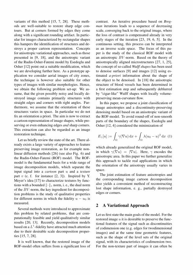
differentiable structure and provides enough free-dom for typical configurations in images with ac-centuated edges, as in aerial images of urban re-gions. Let us first assume a fixed preferred align-

The original images scaled to make all noisevisible.

Evolution with the isotropic ROF-method.

Our method without Bregman iterations.

Our method with two Bregman iterations.

Figure 1: Reconstruction of an artificial edge: Inthe top row from left to right are the original im-ages: A clean edge with noise, the same edge ar-tificially destroyed, this destroyed edge with noise.The noise is equally distributed in [−0.3, 0.3]. Theimages have been intensity-scaled to show the fullrange of noise. In the rows beneath we show the re-sults from different methods. One can observe thatthe isotropic ROF method always evolves roundededges whereas our method is able to produce sharpcorners.

ment of edges, namely horizontal and vertical struc-tures. In this case, the anisotropy would be ex-pressed by

γ(z) =

˛„10

«z

˛+

˛„01

«z

˛= |z1|+ |z2|,

α

α

αq

p

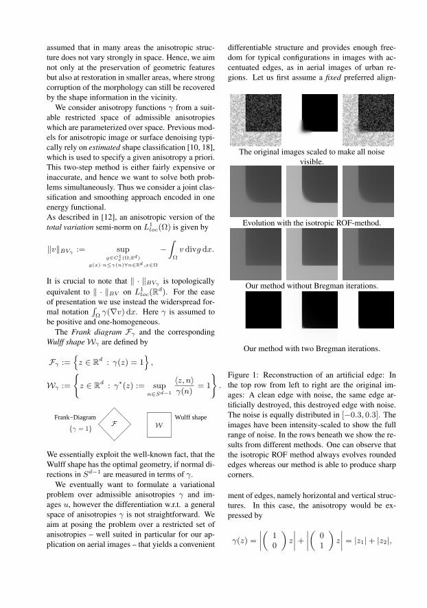
Figure 2: Left: Rotated Wulff shapes overlaying atest example. Right: The definition of p and q.

which is the 1-norm with the unit square as the re-spective Wulff shape.

In order to yield an alignment for arbitrary rightangles we have to rotate the Wulff shape. Conse-quently, we introduce a free parameter α, whichrepresents the angle of the rotation.We confine on the background of our application toa rotated l1-norm as a Wulff shape and are inter-ested in structures with right angles and an orienta-tion given by an angle α. Therefore we introduce avector p = p(α) which is collinear to the base lineof the Wulff shape and a vector q = q(α) which isorthogonal to it (see Figure 2):

p(α) :=

„cos αsin α

«, q(α) :=

„− sin αcos α

«.

We denote by M(α) :=

„cos α sin α− sin α cos α

«the

orthogonal matrix for a rotation by −α. This leadsto the anisotropic energy

Eγ [u, α] :=λ

s

ZΩ

|u−u0|s dx+

ZΩ

|M(α)∇u|1 dx,

where 1 ≤ s < ∞. Typical choices are s = 2 ors = 1. Furthermore, we have to control the varia-tion of the free parameter α. Recall, that the focusof the proposed restoration method is the treatmentof corners, which are co-dimension two objects. Incase of a simple Dirichlet type regularization, wewould observe a lack of regularity from the Sobolevembedding theorem. Thus, we consider a higher or-der regularization energy, namely:

Eα[α] :=

ZΩ

1

2

`µ1|∇α|2 + µ2|∆α|2

´dx.

Now, the total energy to be minimized is given by

E[u, α] = Eγ [u, α] + Eα[α].

The first term of the energy Eγ ensures, that theevolution does not differ too much from the orig-inal image, the second term is the rotated 1-normtaking care of the prefered shapes. Furthermore, theenergy Eα limits the spatial variations of the orien-tation parameter α.

Let us have a closer look at the second term of

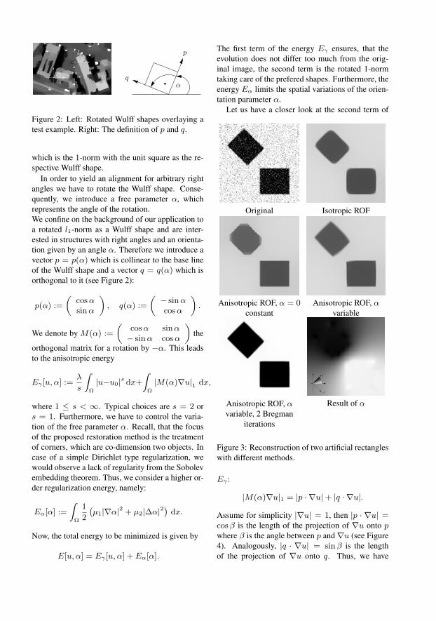
Original Isotropic ROF

Anisotropic ROF, α = 0constant

Anisotropic ROF, αvariable

Anisotropic ROF, αvariable, 2 Bregman

iterations

−π2

π2

Result of α

Figure 3: Reconstruction of two artificial rectangleswith different methods.

Eγ :

|M(α)∇u|1 = |p · ∇u|+ |q · ∇u|.

Assume for simplicity |∇u| = 1, then |p · ∇u| =cos β is the length of the projection of ∇u onto pwhere β is the angle between p and ∇u (see Figure4). Analogously, |q · ∇u| = sin β is the lengthof the projection of ∇u onto q. Thus, we have

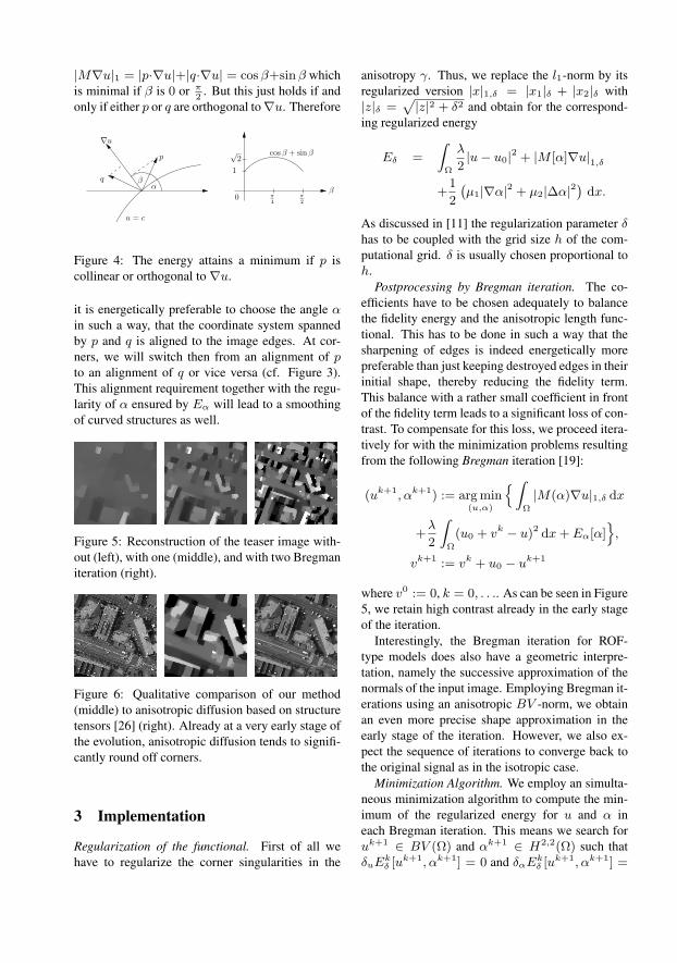
|M∇u|1 = |p·∇u|+|q·∇u| = cos β+sin β whichis minimal if β is 0 or π

2. But this just holds if and

only if either p or q are orthogonal to∇u. Therefore

p

αq

∇u

0

√2

1

π2

π4

cos β + sin β

ββ

u = c

Figure 4: The energy attains a minimum if p iscollinear or orthogonal to ∇u.

it is energetically preferable to choose the angle αin such a way, that the coordinate system spannedby p and q is aligned to the image edges. At cor-ners, we will switch then from an alignment of pto an alignment of q or vice versa (cf. Figure 3).This alignment requirement together with the regu-larity of α ensured by Eα will lead to a smoothingof curved structures as well.

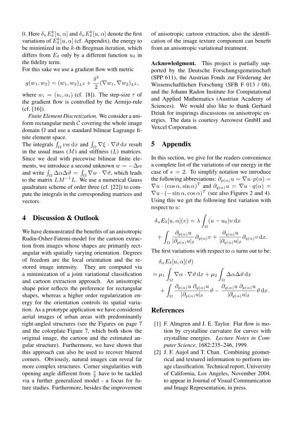
Figure 5: Reconstruction of the teaser image with-out (left), with one (middle), and with two Bregmaniteration (right).

Figure 6: Qualitative comparison of our method(middle) to anisotropic diffusion based on structuretensors [26] (right). Already at a very early stage ofthe evolution, anisotropic diffusion tends to signifi-cantly round off corners.

3 Implementation

Regularization of the functional. First of all wehave to regularize the corner singularities in the

anisotropy γ. Thus, we replace the l1-norm by itsregularized version |x|1,δ = |x1|δ + |x2|δ with|z|δ =

p|z|2 + δ2 and obtain for the correspond-

ing regularized energy

Eδ =

ZΩ

λ

2|u− u0|2 + |M [α]∇u|1,δ

+1

2

`µ1|∇α|2 + µ2|∆α|2

´dx.

As discussed in [11] the regularization parameter δhas to be coupled with the grid size h of the com-putational grid. δ is usually chosen proportional toh.

Postprocessing by Bregman iteration. The co-efficients have to be chosen adequately to balancethe fidelity energy and the anisotropic length func-tional. This has to be done in such a way that thesharpening of edges is indeed energetically morepreferable than just keeping destroyed edges in theirinitial shape, thereby reducing the fidelity term.This balance with a rather small coefficient in frontof the fidelity term leads to a significant loss of con-trast. To compensate for this loss, we proceed itera-tively for with the minimization problems resultingfrom the following Bregman iteration [19]:

(uk+1, αk+1) := arg min(u,α)

n ZΩ

|M(α)∇u|1,δ dx

+λ

2

ZΩ

(u0 + vk − u)2 dx + Eα[α]o

,

vk+1 := vk + u0 − uk+1

where v0 := 0, k = 0, . . .. As can be seen in Figure5, we retain high contrast already in the early stageof the iteration.

Interestingly, the Bregman iteration for ROF-type models does also have a geometric interpre-tation, namely the successive approximation of thenormals of the input image. Employing Bregman it-erations using an anisotropic BV -norm, we obtainan even more precise shape approximation in theearly stage of the iteration. However, we also ex-pect the sequence of iterations to converge back tothe original signal as in the isotropic case.

Minimization Algorithm. We employ an simulta-neous minimization algorithm to compute the min-imum of the regularized energy for u and α ineach Bregman iteration. This means we search foruk+1 ∈ BV (Ω) and αk+1 ∈ H2,2(Ω) such thatδuEk

δ [uk+1, αk+1] = 0 and δαEkδ [uk+1, αk+1] =

0. Here δuEkδ [u, α] and δαEk

δ [u, α] denote the firstvariations of Ek

δ [u, α] (cf. Appendix), the energy tobe minimized in the k-th Bregman iteration, whichdiffers from Eδ only by a different function u0 inthe fidelity term.For this sake we use a gradient flow with metric

g(w1, w2) = (w1, w2)L2 +δ2

2(∇w1,∇w2)L2 ,

where wi = (ui, αi) (cf. [8]). The step-size τ ofthe gradient flow is controlled by the Armijo-rule(cf. [16]).

Finite Element Discretization. We consider a uni-form rectangular mesh C covering the whole imagedomain Ω and use a standard bilinear Lagrange fi-nite element space.The integrals

RΩ

vw dx andRΩ∇ξ · ∇ϑ dx result

in the usual mass (M ) and stiffness (L) matrices.Since we deal with piecewise bilinear finite ele-ments, we introduce a second unknown w = −∆αand write

RΩ

∆α∆ϑ =RΩ∇w · ∇ϑ, which leads

to the matrix LM−1L. We use a numerical Gaussquadrature scheme of order three (cf. [22]) to com-pute the integrals in the corresponding matrices andvectors.

4 Discussion & Outlook

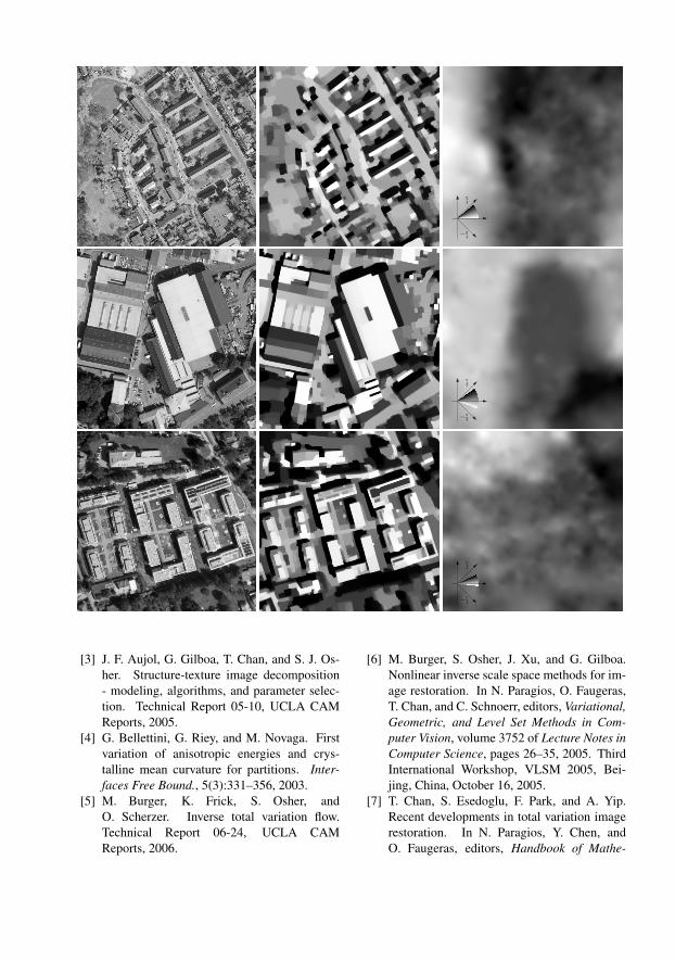
We have demonstrated the benefits of an anisotropicRudin-Osher-Fatemi-model for the cartoon extrac-tion from images whose shapes are primarily rect-angular with spatially varying orientation. Degreesof freedom are the local orientation and the re-stored image intensity. They are computed viaa minimization of a joint variational classificationand cartoon extraction approach. An anisotropicshape prior reflects the preference for rectangularshapes, whereas a higher order regularization en-ergy for the orientation controls its spatial varia-tion. As a prototype application we have consideredaerial images of urban areas with predominantlyright-angled structures (see the Figures on page 7and the colorplate Figure 7, which both show theoriginal image, the cartoon and the estimated an-gular structure). Furthermore, we have shown thatthis approach can also be used to recover blurredcorners. Obviously, natural images can reveal farmore complex structures. Corner singularities withopening angle different from π

2have to be tackled

via a further generalized model - a focus for fu-ture studies. Furthermore, besides the improvement

of anisotropic cartoon extraction, also the identifi-cation of the image texture component can benefitfrom an anisotropic variational treatment.

Acknowledgment. This project is partially sup-ported by the Deutsche Forschungsgemeinschaft(SPP 611), the Austrian Fonds zur Forderung derWissenschaftlichen Forschung (SFB F 013 / 08),and the Johann Radon Institute for Computationaland Applied Mathematics (Austrian Academy ofSciences). We would also like to thank GerhardDziuk for inspirings discussions on anisotropic en-ergies. The data is courtesy Aerowest GmbH andVexcel Corporation.

5 Appendix

In this section, we give for the readers conveniencea complete list of the variations of our energy in thecase of s = 2. To simplify notation we introducethe following abbreviations: ∂p(α)u = ∇u·p(α) =∇u · (cos α, sin α)T and ∂q(α)u = ∇u · q(α) =∇u · (− sin α, cos α)T (see also Figures 2 and 4).Using this we get the following first variation withrespect to u:

δuEδ[u, α](v) = λ

ZΩ

(u− u0)v dx

+

ZΩ

∂p(α)u

|∂p(α)u|δ∂p(α)v +

∂q(α)u

|∂q(α)u|δ∂q(α)v dx.

The first variations with respect to α turns out to be:

δαEδ[u, α](ϑ)

= µ1

ZΩ

∇α · ∇ϑ dx + µ2

ZΩ

∆α∆ϑ dx

+

ZΩ

∂p(α)u ∂q(α)u

|∂p(α)u|δϑ−

∂q(α)u ∂p(α)u

|∂q(α)u|δϑ dx.

References

[1] F. Almgren and J. E. Taylor. Flat flow is mo-tion by crystalline curvature for curves withcrystalline energies. Lecture Notes in Com-puter Science, 1682:235–246, 1999.

[2] J. F. Aujol and T. Chan. Combining geomet-rical and textured information to perform im-age classification. Technical report, Universityof California, Los Angeles, November 2004.to appear in Journal of Visual Communicationand Image Representation, in press.

−π4

π4

−π4

π4

−π4

π4

[3] J. F. Aujol, G. Gilboa, T. Chan, and S. J. Os-her. Structure-texture image decomposition- modeling, algorithms, and parameter selec-tion. Technical Report 05-10, UCLA CAMReports, 2005.

[4] G. Bellettini, G. Riey, and M. Novaga. Firstvariation of anisotropic energies and crys-talline mean curvature for partitions. Inter-faces Free Bound., 5(3):331–356, 2003.

[5] M. Burger, K. Frick, S. Osher, andO. Scherzer. Inverse total variation flow.Technical Report 06-24, UCLA CAMReports, 2006.

[6] M. Burger, S. Osher, J. Xu, and G. Gilboa.Nonlinear inverse scale space methods for im-age restoration. In N. Paragios, O. Faugeras,T. Chan, and C. Schnoerr, editors, Variational,Geometric, and Level Set Methods in Com-puter Vision, volume 3752 of Lecture Notes inComputer Science, pages 26–35, 2005. ThirdInternational Workshop, VLSM 2005, Bei-jing, China, October 16, 2005.

[7] T. Chan, S. Esedoglu, F. Park, and A. Yip.Recent developments in total variation imagerestoration. In N. Paragios, Y. Chen, andO. Faugeras, editors, Handbook of Mathe-

matical Models in Computer Vision. Springer,2004.

[8] U. Clarenz, M. Droske, and M. Rumpf. To-wards fast non–rigid registration. In InverseProblems, Image Analysis and Medical Imag-ing, AMS Special Session Interaction of In-verse Problems and Image Analysis, volume313, pages 67–84. AMS, 2002.

[9] U. Clarenz, G. Dziuk, and M. Rumpf. On gen-eralized mean curvature flow in surface pro-cessing. In H. Karcher and S. Hildebrandt, ed-itors, Geometric analysis and nonlinear par-tial differential equations, pages 217–248.Springer, 2003.

[10] U. Clarenz, M. Rumpf, and A. Telea. Ro-bust feature detection and local classificationfor surfaces based on moment analysis. IEEETransactions on Visualization and ComputerGraphics, 10(5):516–524, 2004.

[11] K. Deckelnick and G. Dziuk. Numerical ap-proximation of mean curvature flow of graphsand level sets. In P. Colli and J. F. Rodrigues,editors, Mathematical Aspects of Evolving In-terfaces, Madeira, Funchal, Portugal, 2000.Lecture Notes in Mathematics, volume 1812,pages 53–87. Springer-Verlag Berlin Heidel-berg, 2003.

[12] Selim Esedoglu and Stanley J. Osher. Decom-position of images by the anisotropic Rudin-Osher-Fatemi model. Comm. Pure Appl.Math., 57(12):1609–1626, 2004.

[13] J. B. Garnett, T. M. Le, and L. A. Vese. Imagedecompositions using bounded variation andhomogeneous besov spaces. Technical Report05-57, UCLA CAM Reports, 2005.

[14] A. Haddad and Y. Meyer. Variational methodsin image processing. Technical Report 04-52,UCLA CAM Reports, 2004.

[15] A. Haddad and S. Osher. Texture separationBV − G and BV − L1. Technical Report06-26, UCLA CAM reports, 2006.

[16] P. Kosmol. Optimierung und Approximation.de Gruyter Lehrbuch, 1991.

[17] Y. Meyer. Oscillating Patterns in Image Pro-cessing and Nonlinear Evolution Equations,volume 22 of University Lecture Series. AMS,2001.

[18] O. Nemitz, M. Rumpf, T. Tasdizen, andR. Whitaker. Anisotropic curvature motionfor structure enhancing smoothing of 3D MR

angiography data. Journal of MathematicalImaging and Vision, May 2006. to appear.

[19] S. J. Osher, M. Burger, D. Goldfarb, J. Xu, andW. Yin. An iterative regularization methodfor total variation-based image restoration.SIAM Multiscale, Modeling and Simulation,4(2):460–489, 2005.

[20] S. J. Osher, A. Sole, and L. A. Vese. Image de-composition and restoration using total varia-tion minimization and the H−1 norm. Techni-cal Report 02-57, UCLA CAM Reports, 2002.

[21] L. Rudin, S. Osher, and E. Fatemi. Nonlineartotal variation based noise-removal. PhysicaD, 60:259–268, 1992.

[22] R. Schaback and H. Werner. NumerischeMathematik. Springer-Verlag, Berlin, 4teAufl. edition, 1992.

[23] O. Scherzer and C.W. Groetsch. Inversescale space theory for inverse problems. Lec-ture Notes in Computer Science, Springer,2106:317–325, 2001.

[24] J. Shen. Piecewise H−1 + H0 + H1 im-ages and the Mumford-Shah-Sobolev modelfor segmented image decomposition. AppliedMath. Research Exp., 4:143–167, 2005.

[25] J. E. Taylor, J. W. Cahn, and W. C. Carter.Variational methods for microstructural evo-lution. JOM, 49(12):30–36, 1998.

[26] J. Weickert. Anisotropic diffusion in imageprocessing. Teubner, 1998.

[27] G. Wulff. Zur Frage der Geschwindigkeitdes Wachstums und der Auflosung derKristallflachen. Zeitschrift der Kristallogra-phie, 34:449–530, 1901.

[28] W. Yin, D. Goldfarb, and S. J. Osher. Imagecartoon-texture decomposition and feature se-lection using the total variation regularized L1

functional. Technical Report 05-47, UCLACAM Reports, 2005.

−π4

π4

−π4

π4

−π4

π4

−π4

π4

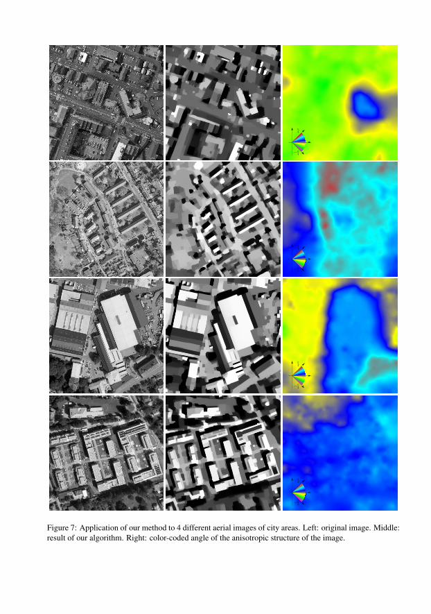
Figure 7: Application of our method to 4 different aerial images of city areas. Left: original image. Middle:result of our algorithm. Right: color-coded angle of the anisotropic structure of the image.