Image processing using Arithmetic Operations

IT523:DIP - Lecture 3

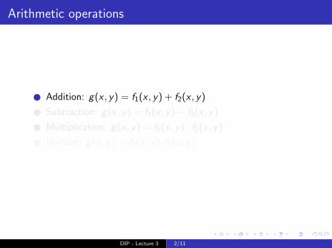
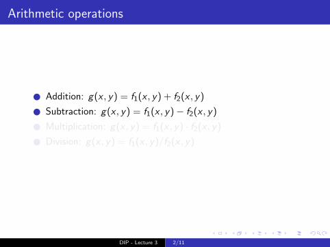
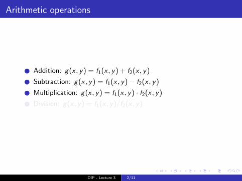
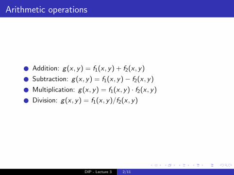
Arithmetic operations

Addition: g(x , y) = f1(x , y) + f2(x , y)

Subtraction: g(x , y) = f1(x , y)− f2(x , y)

Multiplication: g(x , y) = f1(x , y) · f2(x , y)

Division: g(x , y) = f1(x , y)/f2(x , y)

DIP - Lecture 3 2/11

Arithmetic operations

Addition: g(x , y) = f1(x , y) + f2(x , y)

Subtraction: g(x , y) = f1(x , y)− f2(x , y)

Multiplication: g(x , y) = f1(x , y) · f2(x , y)

Division: g(x , y) = f1(x , y)/f2(x , y)

DIP - Lecture 3 2/11

Arithmetic operations

Addition: g(x , y) = f1(x , y) + f2(x , y)

Subtraction: g(x , y) = f1(x , y)− f2(x , y)

Multiplication: g(x , y) = f1(x , y) · f2(x , y)

Division: g(x , y) = f1(x , y)/f2(x , y)

DIP - Lecture 3 2/11

Arithmetic operations

Addition: g(x , y) = f1(x , y) + f2(x , y)

Subtraction: g(x , y) = f1(x , y)− f2(x , y)

Multiplication: g(x , y) = f1(x , y) · f2(x , y)

Division: g(x , y) = f1(x , y)/f2(x , y)

DIP - Lecture 3 2/11

Addition

Given that additive noise corrupts the imagef (x , y) = g(x , y) + η(x , y), where η is also assumed to beuncorrelated at every pixel (x , y) and has zero mean.

Capture N images{fi (x , y) = g(x , y) + ηi (x , y), i = 1, . . . ,N}.

Averaging images: g̃(x , y) = 1N

∑Ni=1 fi (x , y).

Unbiased estimator: E{g̃(x , y)} = g(x , y)

Variance σ2g̃(x ,y) = 1Nσ

2η(x ,y).

DIP - Lecture 3 3/11

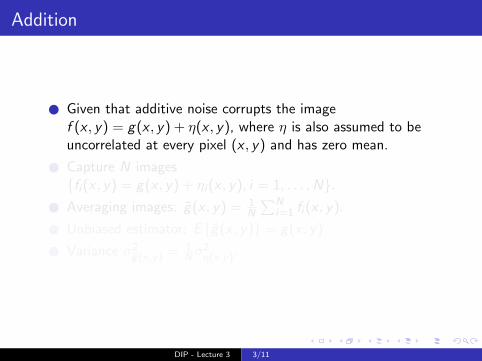
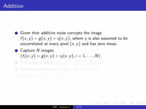
Addition

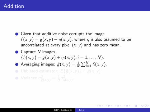
Given that additive noise corrupts the imagef (x , y) = g(x , y) + η(x , y), where η is also assumed to beuncorrelated at every pixel (x , y) and has zero mean.

Capture N images{fi (x , y) = g(x , y) + ηi (x , y), i = 1, . . . ,N}.

Averaging images: g̃(x , y) = 1N

∑Ni=1 fi (x , y).

Unbiased estimator: E{g̃(x , y)} = g(x , y)

Variance σ2g̃(x ,y) = 1Nσ

2η(x ,y).

DIP - Lecture 3 3/11

Addition

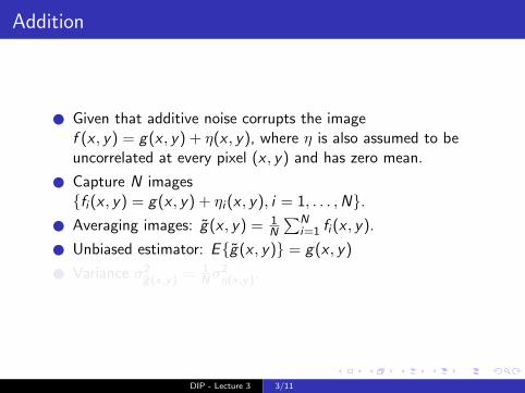
Given that additive noise corrupts the imagef (x , y) = g(x , y) + η(x , y), where η is also assumed to beuncorrelated at every pixel (x , y) and has zero mean.

Capture N images{fi (x , y) = g(x , y) + ηi (x , y), i = 1, . . . ,N}.

Averaging images: g̃(x , y) = 1N

∑Ni=1 fi (x , y).

Unbiased estimator: E{g̃(x , y)} = g(x , y)

Variance σ2g̃(x ,y) = 1Nσ

2η(x ,y).

DIP - Lecture 3 3/11

Addition

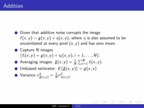
Given that additive noise corrupts the imagef (x , y) = g(x , y) + η(x , y), where η is also assumed to beuncorrelated at every pixel (x , y) and has zero mean.

Capture N images{fi (x , y) = g(x , y) + ηi (x , y), i = 1, . . . ,N}.

Averaging images: g̃(x , y) = 1N

∑Ni=1 fi (x , y).

Unbiased estimator: E{g̃(x , y)} = g(x , y)

Variance σ2g̃(x ,y) = 1Nσ

2η(x ,y).

DIP - Lecture 3 3/11

Addition

Given that additive noise corrupts the imagef (x , y) = g(x , y) + η(x , y), where η is also assumed to beuncorrelated at every pixel (x , y) and has zero mean.

Capture N images{fi (x , y) = g(x , y) + ηi (x , y), i = 1, . . . ,N}.

Averaging images: g̃(x , y) = 1N

∑Ni=1 fi (x , y).

Unbiased estimator: E{g̃(x , y)} = g(x , y)

Variance σ2g̃(x ,y) = 1Nσ

2η(x ,y).

DIP - Lecture 3 3/11

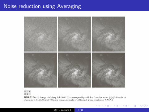
Noise reduction using Averaging

DIP - Lecture 3 4/11

Subtraction

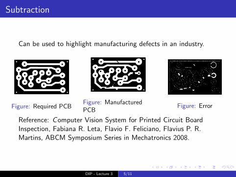
Can be used to highlight manufacturing defects in an industry.

Figure: Required PCBFigure: ManufacturedPCB

Figure: Error

Reference: Computer Vision System for Printed Circuit BoardInspection, Fabiana R. Leta, Flavio F. Feliciano, Flavius P. R.Martins, ABCM Symposium Series in Mechatronics 2008.

DIP - Lecture 3 5/11

Image interpolation (Digital zoom)

Technically, it deals with estimating/creating data at locationswhere it is unknown.

Simple schemes:

� Pixel replication: If the magnification factor is an integermultiple simply copy grey values to neighboring unknownpixels.

DIP - Lecture 3 6/11

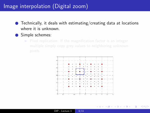
Image interpolation (Digital zoom)

Technically, it deals with estimating/creating data at locationswhere it is unknown.

Simple schemes:

� Pixel replication: If the magnification factor is an integermultiple simply copy grey values to neighboring unknownpixels.

DIP - Lecture 3 6/11

Image interpolation (Digital zoom)

Technically, it deals with estimating/creating data at locationswhere it is unknown.

Simple schemes:

� Pixel replication: If the magnification factor is an integermultiple simply copy grey values to neighboring unknownpixels.

DIP - Lecture 3 6/11

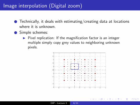
Image interpolation (Digital zoom)

Technically, it deals with estimating/creating data at locationswhere it is unknown.

Simple schemes:

� Pixel replication: If the magnification factor is an integermultiple simply copy grey values to neighboring unknownpixels.

DIP - Lecture 3 6/11

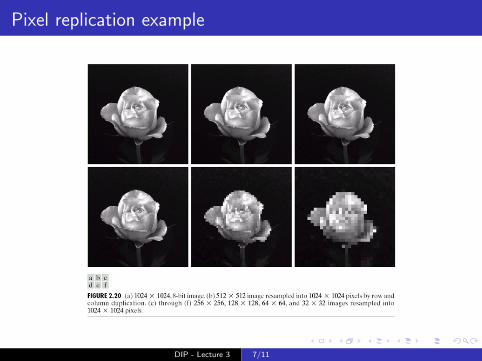
Pixel replication example

DIP - Lecture 3 7/11

Nearest neighbor interpolation

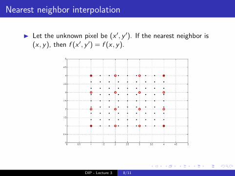
� Let the unknown pixel be (x ′, y ′). If the nearest neighbor is(x , y), then f (x ′, y ′) = f (x , y).

DIP - Lecture 3 8/11

Nearest neighbor interpolation

� Let the unknown pixel be (x ′, y ′). If the nearest neighbor is(x , y), then f (x ′, y ′) = f (x , y).

DIP - Lecture 3 8/11

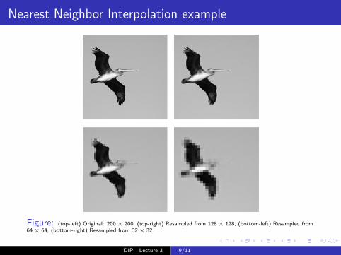
Nearest Neighbor Interpolation example

Figure: (top-left) Original: 200 × 200, (top-right) Resampled from 128 × 128, (bottom-left) Resampled from64 × 64, (bottom-right) Resampled from 32 × 32

DIP - Lecture 3 9/11

Bilinear interpolation

Assume the image satisfies the following rule within the 4nearest neighbors of the point (x ′, y ′):

f (x , y) = ax + by + cxy + d

Since f is known at 4 points, we can solve a 4× 4 linearsystem of equations to get a, b, c , d . Use the above equationwith these coefficients to compute f (x ′, y ′).

DIP - Lecture 3 10/11

Bilinear interpolation

Assume the image satisfies the following rule within the 4nearest neighbors of the point (x ′, y ′):

f (x , y) = ax + by + cxy + d

Since f is known at 4 points, we can solve a 4× 4 linearsystem of equations to get a, b, c , d . Use the above equationwith these coefficients to compute f (x ′, y ′).

DIP - Lecture 3 10/11

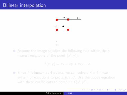
Bilinear interpolation

Assume the image satisfies the following rule within the 4nearest neighbors of the point (x ′, y ′):

f (x , y) = ax + by + cxy + d

Since f is known at 4 points, we can solve a 4× 4 linearsystem of equations to get a, b, c , d . Use the above equationwith these coefficients to compute f (x ′, y ′).

DIP - Lecture 3 10/11

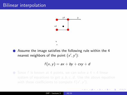
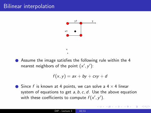
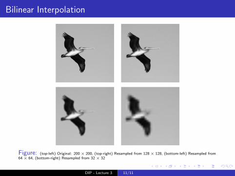
Bilinear Interpolation

Figure: (top-left) Original: 200 × 200, (top-right) Resampled from 128 × 128, (bottom-left) Resampled from64 × 64, (bottom-right) Resampled from 32 × 32

DIP - Lecture 3 11/11