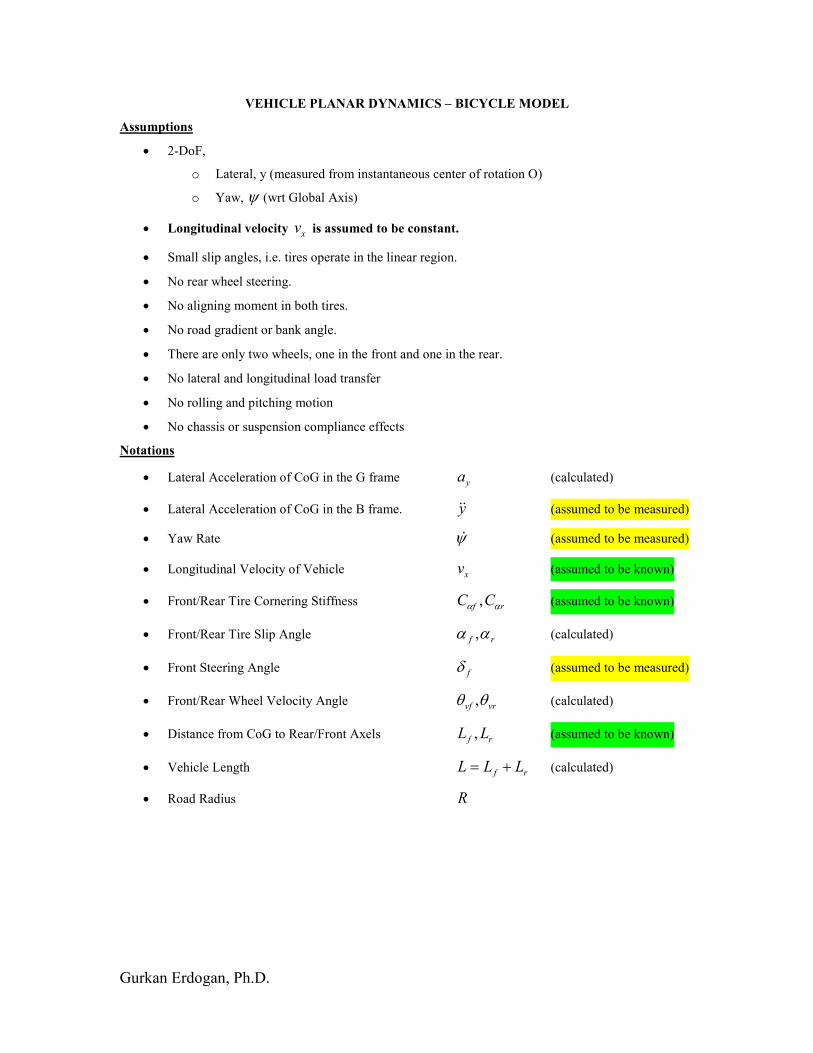
Gurkan Erdogan, Ph.D.

VEHICLE PLANAR DYNAMICS – BICYCLE MODEL

Assumptions

• 2-DoF,

o Lateral, y (measured from instantaneous center of rotation O)

o Yaw, ψ (wrt Global Axis)

• Longitudinal velocity xv is assumed to be constant.

• Small slip angles, i.e. tires operate in the linear region.

• No rear wheel steering.

• No aligning moment in both tires.

• No road gradient or bank angle.

• There are only two wheels, one in the front and one in the rear.

• No lateral and longitudinal load transfer

• No rolling and pitching motion

• No chassis or suspension compliance effects

Notations

• Lateral Acceleration of CoG in the G frame ya (calculated)

• Lateral Acceleration of CoG in the B frame. y&& (assumed to be measured)

• Yaw Rate ψ& (assumed to be measured)

• Longitudinal Velocity of Vehicle xv (assumed to be known)

• Front/Rear Tire Cornering Stiffness rf CC αα , (assumed to be known)

• Front/Rear Tire Slip Angle rf αα , (calculated)

• Front Steering Angle fδ (assumed to be measured)

• Front/Rear Wheel Velocity Angle vrvf θθ , (calculated)

• Distance from CoG to Rear/Front Axels rf LL , (assumed to be known)

• Vehicle Length rf LLL += (calculated)

• Road Radius R

Gurkan Erdogan, Ph.D.

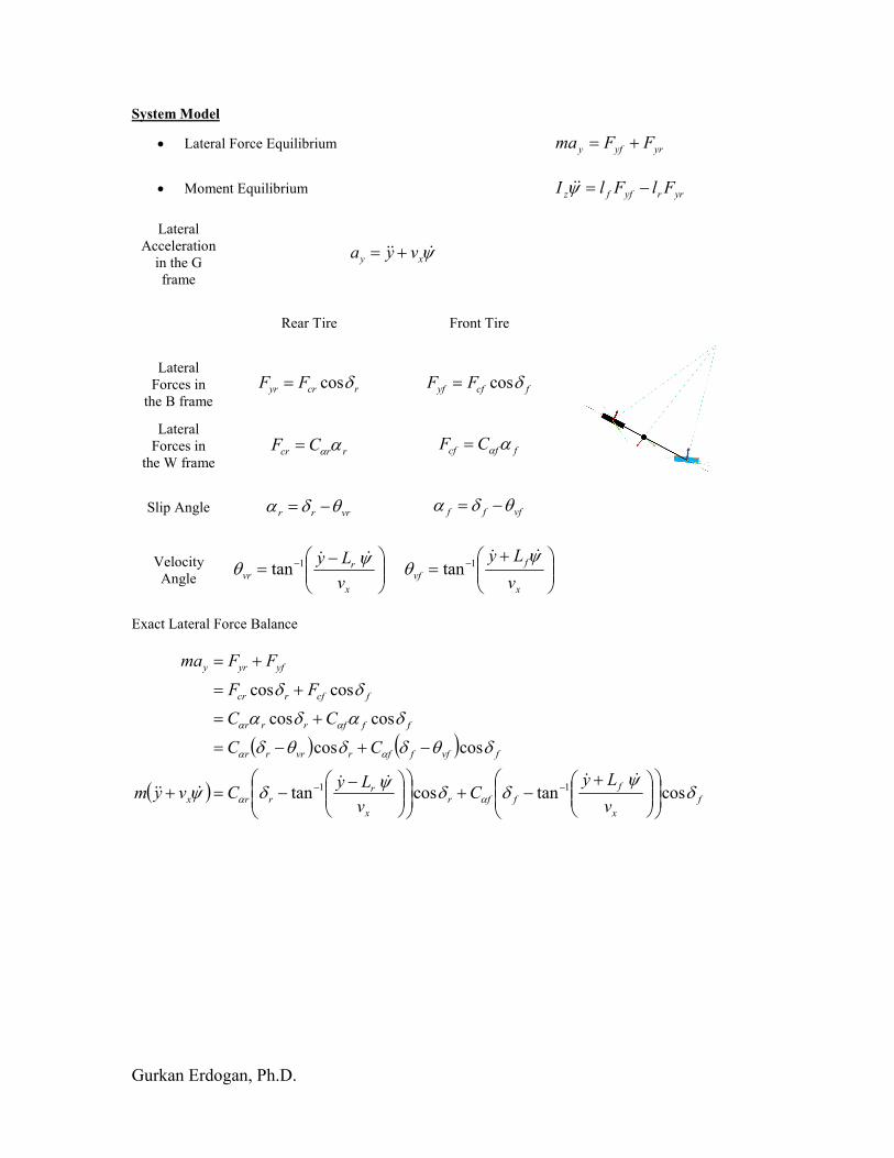
System Model

• Lateral Force Equilibrium yryfy FFma +=

• Moment Equilibrium yrryffz FlFlI −=ψ&&

Lateral

Acceleration

in the G

frame

ψ&&&xy vya +=

Rear Tire Front Tire

Lateral

Forces in

the B frame rcryr FF δcos= fcfyf FF δcos=

Lateral

Forces in

the W frame rrcr CF αα= ffcf CF αα=

Slip Angle vrrr θδα −= vfff θδα −=

Velocity

Angle

−= −

x

rvr

v

Ly ψθ

&&1tan

+= −

x

f

vfv

Ly ψθ

&&1tan

Exact Lateral Force Balance

( ) ( )

( ) f

x

f

ffr

x

rrrx

fvfffrvrrr

fffrrr

fcfrcr

yfyry

v

LyC

v

LyCvym

CC

CC

FF

FFma

δψ

δδψ

δψ

δθδδθδ

δαδα

δδ

αα

αα

αα

costancostan

coscos

coscos

coscos

11

+−+

−−=+

−+−=

+=

+=

+=

−−&&&&

&&&

Gurkan Erdogan, Ph.D.

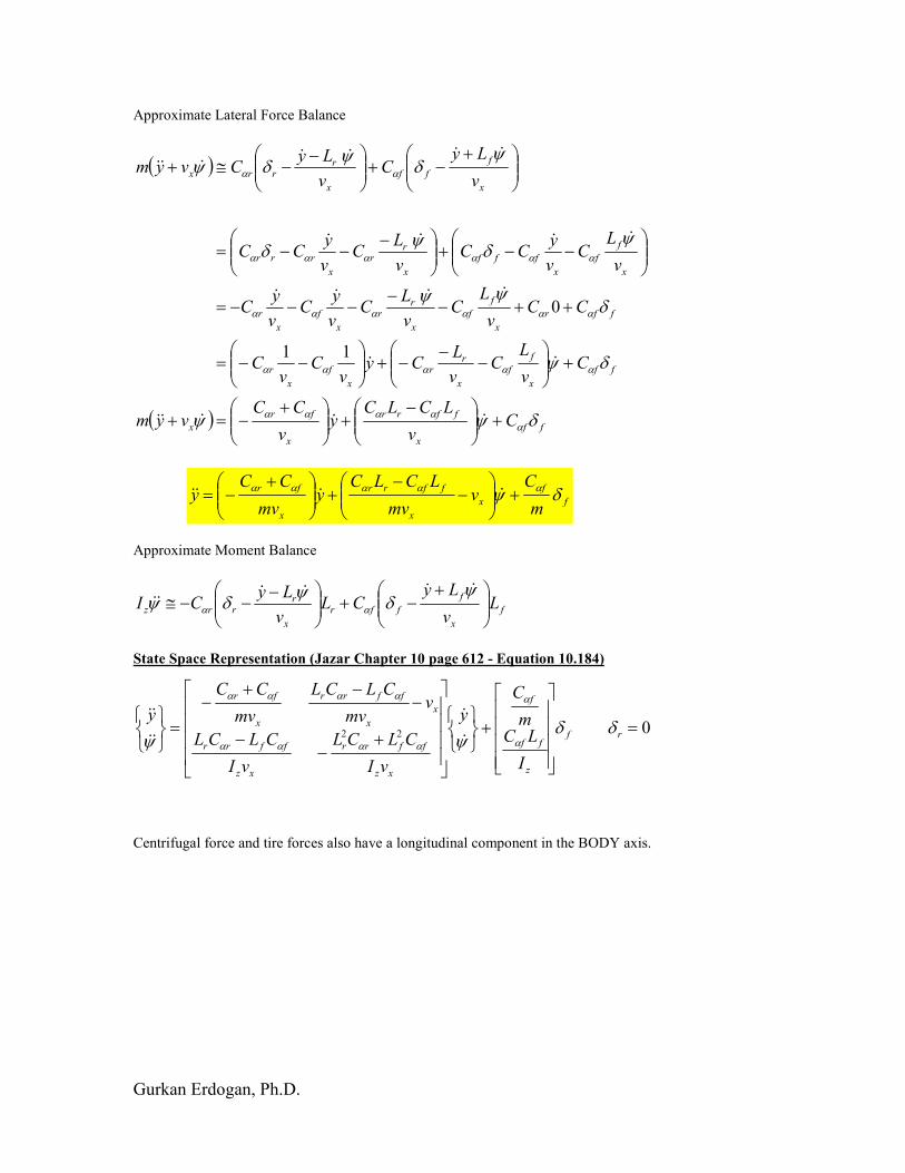
Approximate Lateral Force Balance

( )

( ) ff

x

ffrr

x

fr

x

ff

x

f

f

x

rr

x

f

x

r

ffr

x

f

f

x

rr

x

f

x

r

x

f

f

x

fff

x

rr

x

rrr

x

f

ff

x

rrrx

Cv

LCLCy

v

CCvym

Cv

LC

v

LCy

vC

vC

CCv

LC

v

LC

v

yC

v

yC

v

LC

v

yCC

v

LC

v

yCC

v

LyC

v

LyCvym

δψψ

δψ

δψψ

ψδ

ψδ

ψδ

ψδψ

ααααα

ααααα

αααααα

αααααα

αα

+

−+

+−=+

+

−

−−+

−−=

++−−

−−−=

−−+

−−−=

+−+

−−≅+

&&&&&

&&

&&&&

&&&&

&&&&&&&

11

0

f

f

x

x

ffrr

x

fr

m

Cv

mv

LCLCy

mv

CCy δψ ααααα +

−

−+

+−= &&&&

Approximate Moment Balance

f

x

f

ffr

x

rrrz L

v

LyCL

v

LyCI

+−+

−−−≅

ψδ

ψδψ αα

&&&&&&

State Space Representation (Jazar Chapter 10 page 612 - Equation 10.184)

022 =

+

+−

−

−−+

−

=

rf

z

ff

f

xz

ffrr

xz

ffrr

x

x

ffrr

x

fr

I

LCm

C

y

vI

CLCL

vI

CLCL

vmv

CLCL

mv

CC

yδδ

ψψ α

α

αααα

αααα

&

&

&&

&&

Centrifugal force and tire forces also have a longitudinal component in the BODY axis.

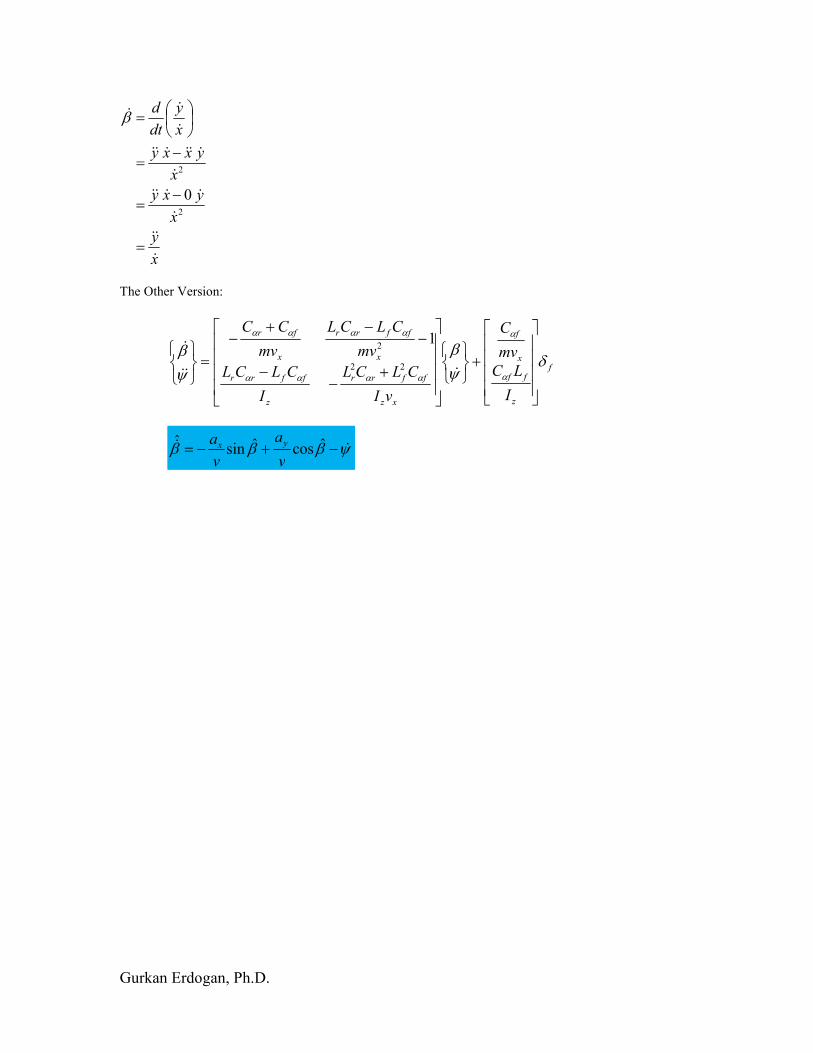
Gurkan Erdogan, Ph.D.

x

y

x

yxy

x

yxxy

x

y

dt

d

&

&&

&

&&&&

&

&&&&&&

&

&&

=

−=

−=

=

2

2

0

β

The Other Version:

f

z

ff

x

f

xz

ffrr

z

ffrr

x

ffrr

x

fr

I

LC

mv

C

vI

CLCL

I

CLCL

mv

CLCL

mv

CC

δψβ

ψβ

α

α

αααα

αααα

+

+−

−

−−+

−

=

&&&

&

22

21

ψβββ && −+−= ˆcosˆsinˆ

v

a

v

a yx

Gurkan Erdogan, Ph.D.

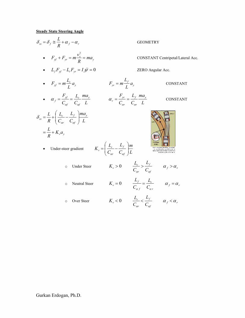
Steady State Steering Angle

rffssR

Lααδδ −+≅= GEOMETRY

• yx

yryf maR

vmFF ==+

2

CONSTANT Centripetal/Lateral Acc.

• 0==− ψ&&zyrryff IFLFL ZERO Angular Acc.

• yr

yf aL

LmF = y

f

yr aL

LmF = CONSTANT

• L

ma

C

L

C

F y

f

r

f

yf

f

αα

α == L

ma

C

L

C

F y

r

f

r

yr

r

αα

α == CONSTANT

yv

y

f

f

r

rss

aKR

L

L

ma

C

L

C

L

R

L

+=

−+=

αα

δ

• Under-steer gradient L

m

C

L

C

LK

f

f

r

rv

−=

αα

o Under Steer rf

f

f

r

rv

C

L

C

LK αα

αα

>>> 0

o Neutral Steer rf

r

r

f

f

vC

L

C

LK αα

αα

=== 0

o Over Steer rf

f

f

r

rv

C

L

C

LK αα

αα

<<< 0

Gurkan Erdogan, Ph.D.

Vehicle Side Slip Angle Estimation

2

ˆ

x

yxxy

x

y

dt

d

&

&&&&&&

&

&&

−=

=β

This looks okay, but we would like to use sensor measurements.

( )

( )

( )

( )

ψββ

ψβψ

βψ

ψβψ

ββψ

β

ψβψββψβ

ψβψβψββ

ψββψββ

ψψββ

ββ

β

&

&&&&&&&&&

&&&&&&&&&

&&&&

&&&

&&&&&&&

&&&&&&

&&&&&&

&&&&

&&&

&&&

&&&&&&

&

&&&&&&&

&

&&&&&&&

−+−=

−+

+−

−=

−+++−=

−+++−=

−+++−=

−+++−=

−++−=

−=

−=

−=

−≅

−=

cossin

cossin

coscossinsin

coscossinsin

cossincossin

cossincossin

cossin

sincos1

1

1

ˆ

22

22

22

2

22

2

2

v

a

v

a

v

xy

v

yx

v

x

v

y

v

y

v

x

v

y

v

x

v

y

v

x

v

y

v

x

v

y

v

x

xyv

v

yx

v

xy

v

yxxyv

x

yxxy

v

x

x

yxxy

yx

Now we can use yaw rate and acceleration sensors to estimate the yaw rate as below.

ψβββ && −+−= ˆcosˆsinˆ

v

a

v

a yx

Maximum Vehicle Side Slip Angle

It is a saturating function of the characteristic velocity.

( ) ( )

2max

12

2

213

3

21max 32

kvv

kv

vkk

v

vkkvv

chx

ch

x

ch

xchx

=⇒>

+−−−=⇒<

β

β

Gurkan Erdogan, Ph.D.

Yaw Rate Estimation

This is actually the steady state response, i.e. the gain, of the transfer function between

the steering input and the yaw rate output.

+

=

2

2

1ch

x

f

x

v

vL

vδ

ψ&

Derivation of the above equation and the Characteristic Velocity

ψψ

δ

&&xv

x

xxv

x

x

xv

yvss

vKv

L

R

vvK

R

v

v

L

R

vK

R

L

aKR

L

+=

+=

+=

+=

2

+

=

+

=

+=

+=

2

22

11ch

x

ssx

xv

x

ss

xvx

xx

ss

xv

x

ss

v

vL

v

L

vK

v

L

vKL

v

v

L

v

L

vKv

L

δδψ

δψ

δψ

&

&

&

v

chK

Lv =2

Maximum Yaw Rate

( )( )

( )βψ

βψ

ββψ

ββ

ˆsin1

sin10

sincos

sincos

max

max

max

max

xmeasrad

x

xxmeasrad

xx

xymeasrad

aav

ava

avy

aaa

−=

++≅

++=

+=

&

&

&&&

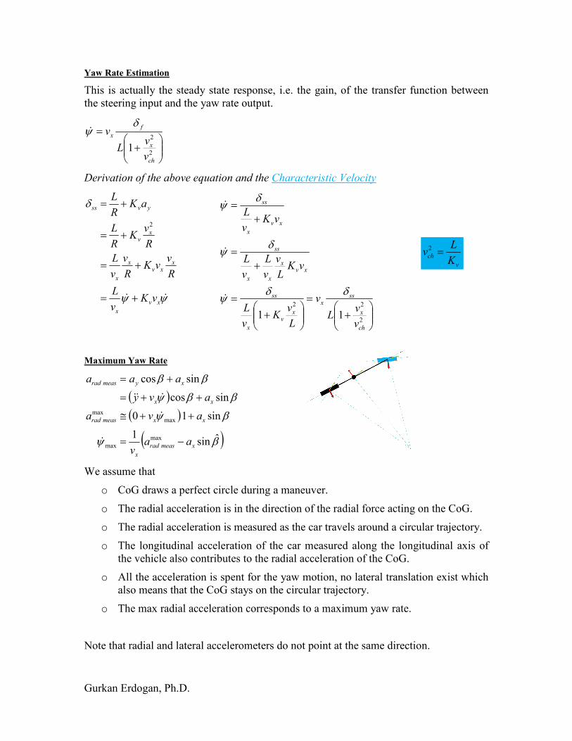
We assume that

o CoG draws a perfect circle during a maneuver.

o The radial acceleration is in the direction of the radial force acting on the CoG.

o The radial acceleration is measured as the car travels around a circular trajectory.

o The longitudinal acceleration of the car measured along the longitudinal axis of

the vehicle also contributes to the radial acceleration of the CoG.

o All the acceleration is spent for the yaw motion, no lateral translation exist which

also means that the CoG stays on the circular trajectory.

o The max radial acceleration corresponds to a maximum yaw rate.

Note that radial and lateral accelerometers do not point at the same direction.

Gurkan Erdogan, Ph.D.

3 tane yerde yaw rate hesapladik

1.Bicycle model steady state

2.Max yawrate Steering Pad deneylerinden

1 ile 2 yi karistirip gaini bulduk sonra bicycle modelin steering input/yaw rate output

(gaini 1 olan) transfer fonksiyonundan gecirdik

(bir adet daha saturation function var en son islem olarak)

3.4W modelden gelen gercege daha yakin yaw rate var birde

Gurkan Erdogan, Ph.D.

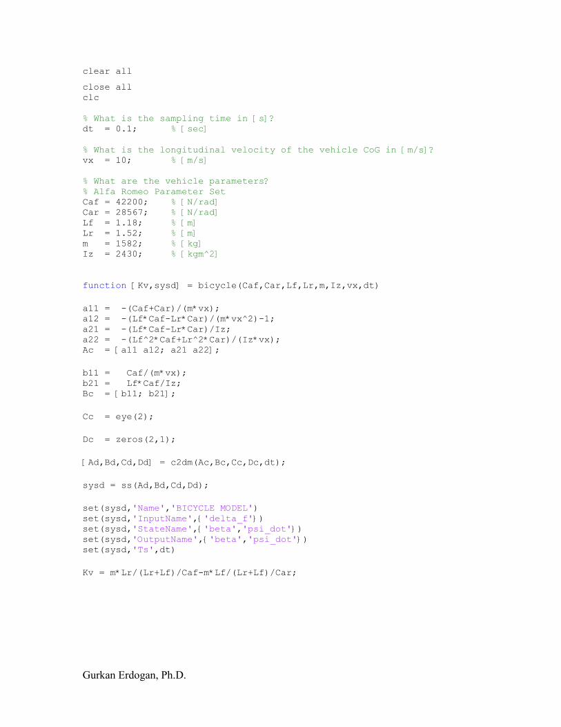
clear all

close all clc % What is the sampling time in [s]? dt = 0.1; % [sec] % What is the longitudinal velocity of the vehicle CoG in [m/s]? vx = 10; % [m/s] % What are the vehicle parameters? % Alfa Romeo Parameter Set Caf = 42200; % [N/rad] Car = 28567; % [N/rad] Lf = 1.18; % [m] Lr = 1.52; % [m] m = 1582; % [kg] Iz = 2430; % [kgm^2]

function [Kv,sysd] = bicycle(Caf,Car,Lf,Lr,m,Iz,vx,dt) a11 = -(Caf+Car)/(m*vx); a12 = -(Lf*Caf-Lr*Car)/(m*vx^2)-1; a21 = -(Lf*Caf-Lr*Car)/Iz; a22 = -(Lf^2*Caf+Lr^2*Car)/(Iz*vx); Ac = [a11 a12; a21 a22]; b11 = Caf/(m*vx); b21 = Lf*Caf/Iz; Bc = [b11; b21]; Cc = eye(2); Dc = zeros(2,1); [Ad,Bd,Cd,Dd] = c2dm(Ac,Bc,Cc,Dc,dt); sysd = ss(Ad,Bd,Cd,Dd); set(sysd,'Name','BICYCLE MODEL') set(sysd,'InputName',{'delta_f'}) set(sysd,'StateName',{'beta','psi_dot'}) set(sysd,'OutputName',{'beta','psi_dot'}) set(sysd,'Ts',dt) Kv = m*Lr/(Lr+Lf)/Caf-m*Lf/(Lr+Lf)/Car;