Universita degli Studi di Roma “La Sapienza”

Dottorato di Ricerca in Ingegneria Informatica

Dipartimento di Informatica e SistemisticaAntonio Ruberti

Jumping around the box:

Graphical and operational studies on

λ-calculus and Linear Logic

Beniamino Accattoli

Advisor :Stefano Guerrini

Referees :Simone MartiniOlivier Laurent

Contents

1 Introduction 71.1 λ-trees, λj-dags and sharing . . . . . . . . . . . . . . . . . . . . . 101.2 The structural λ-calculus . . . . . . . . . . . . . . . . . . . . . . 13

1.2.1 Using λj to revisit λ-calculus . . . . . . . . . . . . . . . . 141.3 Implicit boxes for MELLP . . . . . . . . . . . . . . . . . . . . . . 161.4 General related work . . . . . . . . . . . . . . . . . . . . . . . . . 171.5 Plan of the thesis . . . . . . . . . . . . . . . . . . . . . . . . . . . 19

I λ-calculus 20

2 Graphs for λ-terms 212.1 Hypergraphs and Terms . . . . . . . . . . . . . . . . . . . . . . . 21

2.1.1 Sharing and variables . . . . . . . . . . . . . . . . . . . . 232.2 From terms to graphs . . . . . . . . . . . . . . . . . . . . . . . . 282.3 From graphs to terms . . . . . . . . . . . . . . . . . . . . . . . . 322.4 λ-tree dynamics . . . . . . . . . . . . . . . . . . . . . . . . . . . . 362.5 Variations on a theme . . . . . . . . . . . . . . . . . . . . . . . . 40

2.5.1 Domination criterion(s) . . . . . . . . . . . . . . . . . . . 412.5.2 Switching criterion . . . . . . . . . . . . . . . . . . . . . . 43

3 λ-terms, sharing and jumps 473.1 Introduction . . . . . . . . . . . . . . . . . . . . . . . . . . . . . . 473.2 Sharing and jumps: static . . . . . . . . . . . . . . . . . . . . . . 50

3.2.1 Correctness criterion . . . . . . . . . . . . . . . . . . . . . 523.2.2 λj-boxes . . . . . . . . . . . . . . . . . . . . . . . . . . . . 543.2.3 Read-back of λj-dags . . . . . . . . . . . . . . . . . . . . 583.2.4 Domination criterion . . . . . . . . . . . . . . . . . . . . . 613.2.5 Collapsing Boxes . . . . . . . . . . . . . . . . . . . . . . . 63

3.3 Graphical quotient . . . . . . . . . . . . . . . . . . . . . . . . . . 643.4 Dynamics . . . . . . . . . . . . . . . . . . . . . . . . . . . . . . . 68

3.4.1 The dB-rule . . . . . . . . . . . . . . . . . . . . . . . . . . 693.4.2 The j-rules . . . . . . . . . . . . . . . . . . . . . . . . . . 71

3.5 Terms, graphs and strong bisimulations . . . . . . . . . . . . . . 743.6 Pull-back of the rules . . . . . . . . . . . . . . . . . . . . . . . . . 77

3.6.1 Milner’s rules . . . . . . . . . . . . . . . . . . . . . . . . . 823.7 Appendix: strong bisimulations . . . . . . . . . . . . . . . . . . . 83

3.7.1 Internal strong bisimulation . . . . . . . . . . . . . . . . . 86

2

4 The structural λ-calculus 884.1 Introduction to explicit substitutions . . . . . . . . . . . . . . . . 88

4.1.1 Some ES-calculi . . . . . . . . . . . . . . . . . . . . . . . 904.2 λj: basic properties . . . . . . . . . . . . . . . . . . . . . . . . . 96

4.2.1 Substitutions and Multiplicities . . . . . . . . . . . . . . . 974.2.2 Potential multiplicities, graphically . . . . . . . . . . . . . 1014.2.3 Confluence . . . . . . . . . . . . . . . . . . . . . . . . . . 102

4.3 Preservation of β-Strong Normalization . . . . . . . . . . . . . . 1044.4 Developments and All That . . . . . . . . . . . . . . . . . . . . . 110

4.4.1 Catching L-developments . . . . . . . . . . . . . . . . . . 1134.4.2 XL-developments . . . . . . . . . . . . . . . . . . . . . . . 117

5 λj-dags, Pure Proof-Nets and σ-equivalence 1195.1 Relating λj-dags and Pure Proof-Nets . . . . . . . . . . . . . . . 119

5.1.1 Sequentialization . . . . . . . . . . . . . . . . . . . . . . . 1275.1.2 Dynamics . . . . . . . . . . . . . . . . . . . . . . . . . . . 1305.1.3 Linear head reduction . . . . . . . . . . . . . . . . . . . . 135

5.2 σ-equivalence . . . . . . . . . . . . . . . . . . . . . . . . . . . . . 1375.3 The pure quotient . . . . . . . . . . . . . . . . . . . . . . . . . . 141

5.3.1 Pull-back on λj . . . . . . . . . . . . . . . . . . . . . . . . 145

6 Adding commutative rules to the structural λ-calculus 1476.1 Introduction . . . . . . . . . . . . . . . . . . . . . . . . . . . . . . 147

6.1.1 Introducing the technique . . . . . . . . . . . . . . . . . . 1526.2 Step 1: The Labeled Systems . . . . . . . . . . . . . . . . . . . . 153

6.2.1 Well-Formed Labeled Terms . . . . . . . . . . . . . . . . . 1556.3 Step 2: Labeled IE . . . . . . . . . . . . . . . . . . . . . . . . . . 1586.4 Step 3: Unlabelling . . . . . . . . . . . . . . . . . . . . . . . . . . 159

6.4.1 Some considerations on ≡o and (un)boxing . . . . . . . . 1606.5 Appendix 1: The Forgettable Systems Terminate . . . . . . . . . 162

6.5.1 Termination of →Fb . . . . . . . . . . . . . . . . . . . . . 1646.5.2 Termination of →Fu . . . . . . . . . . . . . . . . . . . . . 166

6.6 Appendix 2: two lemmas and one theorem . . . . . . . . . . . . . 170

7 An experiment 1767.1 Static . . . . . . . . . . . . . . . . . . . . . . . . . . . . . . . . . 1767.2 Dynamics . . . . . . . . . . . . . . . . . . . . . . . . . . . . . . . 1797.3 Empire . . . . . . . . . . . . . . . . . . . . . . . . . . . . . . . . . 180

II Logic 183

8 Paralleliminars: Proof-Nets, Kingdoms, Empires and Polarity 1858.1 Multiplicative Proof-Nets . . . . . . . . . . . . . . . . . . . . . . 186

8.1.1 MLL¬1,⊥ Proof-Nets . . . . . . . . . . . . . . . . . . . . 1888.1.2 Correctness and read-back of MLL¬1,⊥-nets . . . . . . . 1908.1.3 Kingdoms and Empires . . . . . . . . . . . . . . . . . . . 1928.1.4 Adding the constants . . . . . . . . . . . . . . . . . . . . 1968.1.5 The MIX rules . . . . . . . . . . . . . . . . . . . . . . . . . 199

8.2 MELLP . . . . . . . . . . . . . . . . . . . . . . . . . . . . . . . . . 201

3

8.2.1 The system . . . . . . . . . . . . . . . . . . . . . . . . . . 2018.2.2 MELLP Proof-Nets . . . . . . . . . . . . . . . . . . . . . . 2028.2.3 The correctness criterion . . . . . . . . . . . . . . . . . . . 2068.2.4 The polar matching . . . . . . . . . . . . . . . . . . . . . 2088.2.5 Additives and the polarity of the kingdom . . . . . . . . . 210

9 Implicit boxes for cut-free MELLP 2129.1 The idea . . . . . . . . . . . . . . . . . . . . . . . . . . . . . . . . 212

9.1.1 Introducing the system . . . . . . . . . . . . . . . . . . . 2159.2 Correctness criterion . . . . . . . . . . . . . . . . . . . . . . . . . 218

9.2.1 Subnets and implicit boxes . . . . . . . . . . . . . . . . . 2219.2.2 Sequentialization . . . . . . . . . . . . . . . . . . . . . . . 2239.2.3 Collapsing subnets . . . . . . . . . . . . . . . . . . . . . . 224

9.3 Relating implicit boxes and explicit boxes . . . . . . . . . . . . . 226

10 MELLP, cuts and MELLP?d 23010.1 Introducing cuts . . . . . . . . . . . . . . . . . . . . . . . . . . . 23010.2 Jumping cuts . . . . . . . . . . . . . . . . . . . . . . . . . . . . . 233

10.2.1 Subnets and jboxes . . . . . . . . . . . . . . . . . . . . . . 23510.2.2 Sequentialization . . . . . . . . . . . . . . . . . . . . . . . 237

10.3 Dynamics . . . . . . . . . . . . . . . . . . . . . . . . . . . . . . . 24010.4 From MELLP to MELLP?d . . . . . . . . . . . . . . . . . . . . . . 25010.5 Relating jboxes and explicit boxes . . . . . . . . . . . . . . . . . 254

10.5.1 Read-Back . . . . . . . . . . . . . . . . . . . . . . . . . . 25810.5.2 The simulation . . . . . . . . . . . . . . . . . . . . . . . . 25910.5.3 Back to λj . . . . . . . . . . . . . . . . . . . . . . . . . . 26410.5.4 Extension to the additives . . . . . . . . . . . . . . . . . . 266

11 Conclusions and perspectives 26811.1 Implicit boxes and polarity . . . . . . . . . . . . . . . . . . . . . 26811.2 The structural λ-calculus . . . . . . . . . . . . . . . . . . . . . . 27011.3 Future work . . . . . . . . . . . . . . . . . . . . . . . . . . . . . . 270

Bibliography 274

4

Acknowledgements

First of all, I want to thank Stefano Guerrini, my advisor since my undergrad-uate studies. His questions and criticism helped to guide my research and toimprove this work; his suggestions were crucial to the end result. FurthermoreI would like to thank Delia Kesner. She has been another kind advisor. I verymuch enjoyed working with her. Both of them showed me a completely diverseand complementary approach to research. I am glad that I had the chance tolearn from them. Also, I want to thank Stefano and Delia for what went beyondresearch, I admire their personalities as much as I admire them as researchers;they have been truly inspirational to me.

I want to thank Olivier Laurent and Simone Martini for having accepted toact as referees for my thesis, and for the patience they have shown reading thepreliminary version, which was full of typos. I am grateful for Olivier’s workon polarity, in particular for his Ph.D thesis, which I have studied in-depth andkept consulting whenever I had doubts.

Further, I am especially grateful to Roberto Baldoni and Maurizio Lenz-erini, who formed part of the commission accepting me as a Ph.D student.They showed an unusually open mind by giving me a scholarship in computerengineering despite the fact that I had made it clear that I wanted to emphasizeon theoretical and abstract topics. As chairs of the Ph.D program, they allowedme to follow my interests freely.

I also wish to acknowledge Paul-Andre Mellies’ works on rewriting and po-larity, which significantly changed my perspective. Even though there is verylittle trace of his work in this thesis, he had a huge influence on my approach.

A special thank you to Paolo Tranquilli, Paolo Di Giamberardino, DamianoMazza and Michele Pagani. They have taught me a lot about Proof-Nets, and Ialso shared many good moments with them. In particular, I want to thank PaoloTranquilli, whom I experienced as a companion along this journey, and PaoloDi Giamberardino, without whom I probably would never even have consideredjumps. And thank you to Daniel De Carvalho, Marco Gaboardi, Luca Fossatiand Alberto Carraro for the time we have spent together.

I want to thank everyone I met during my two-years stay in the Parisian PPSlab with whom I enjoyed many interesting lunches, breaks and valuable discus-sions. In particular Fabien Renaud, Thibaut Balabonski, Stephane Zimmerman,Antoine Madet, Christine Tasson, Severine Maingaud, Pasquale Lubello, MehdiDogguy, Jonas Frey, Guillaume Munch-Maccagnoni, Pierre Clairambault andSamuel Mimram. Among them a special thank you goes to Antoine Madet,who I often had a good time with outside the lab.

5

Thank you to Andrea Trusiano, Joanna Mederle, Clemente Palopoli, Chris-tian and Heike Fichera, my whole family and in particular my brother Valentinofor their friendship and support during all these years.

Last, I want to thank Irene Hetzenauer. She left her country, family andfriends to accompany me on this adventure. She always supported me andbelieved in me, even at times when I did not. Thank you, Irene, for your love,your positive character, your huge patience during the last months of work, andfor having turned these years into the best ones of my life.

6

Chapter 1

Introduction

Computer Science has been tightly connected to Logic from its very inception:computers are a by-product of the logical investigation on computability of thefirst half of the XXth century. One of the most striking and profound con-nections between the two fields is the Curry-Howard correspondence betweenproofs and programs: proofs of formal deductive systems can be interpreted asprograms in an abstract mathematical form, and vice versa. The paradigmaticexample for such correspondence being the relation between Minimal Intuition-istic Logic and λ-calculus programs.

Both proofs and programs can be endowed with dynamics: programs can beexecuted and proofs can be transformed in ways to avoid the use of intermediaryresults. These two dynamics are notions of computation which, again, are re-lated. The isomorphism between proofs and terms is preserved by computation,i.e., it is dynamic.

Though all this can be stated mathematically, the best evidence we get frompractice: developing a mathematical theory is very much like writing a complexsoftware: modules (lemmas) have to be isolated, variables (hypothesis) have tobe declared, subroutine calls need to match parameters (application of lemmas),the code (the proofs) must be elegant and so forth.

Graphical syntaxes. Proofs and terms are traditionally formalized as treesof instructions (deductive rules) even though two serialized steps preparing theground for some future step are quite often mutually independent: they can bepermuted without affecting the overall result. The study of both disciplines,i.e., proof theory and theoretical approaches to programming languages, hasfound it useful to develop graphical syntaxes for proofs and programs in orderto obtain representations quotienting with respect to such permutations.

The initial idea lies in drawing the different steps on a plane and tryingto connect them by causality. This can already be useful, but in the majorityof cases the representation is not very different from the original. A furtherstep consists in coding notions which are usually coded by means of names insequential proofs/programs with the help of additional edges. As examples wecite the identification of various variable occurrences of the same variable, thelink between a binder and its variable, or the pairing of dual formulas given by

7

axioms. Adding such edges the natural tree-shape of sequential programs andproofs changes to that of general graphs, that is, the geometrical representationgets richer.

The computational rules defining the evaluation of programs can be turnedinto graph transformations. The switch to graphs can make some computa-tional rules useless, like those for instance which simply permute independentdeductive steps, or naturally lead to decompose the rules of the sequential sys-tem into more atomic graphical rules. Necessarily one needs to show that thegraphical computation is coherent with respect to the sequential one, i.e., thatit computes the same results. Studying the interplay of these two dynamics canreveal very interesting properties of computation, and lead to implement par-ticular strategies, like, for instance, the Levy-optimal one (see [AG98]), whichcannot be achieved using sequential representations.

Correctness criterions. A breakthrough in the field of graphical syntaxeshas been the introduction by Jean-Yves Girard of Proof Nets [Gir87], a graphicalsyntax for Linear Logic. Characterizing through a set of geometrical conditions,called a correctness criterion, all and only the graphical objects correspond-ing to the proofs of Linear Logic, he revolutionized the field.

In general, the free language generated by the constructors of a graphicalsyntax, called links, is larger than the sequential language one started with,since there are many graphs which do not correspond to a term, usually becauseof a bad cycle which is not expressible in the sequential world.

A criterion exhibits the mathematical geometrical structure characterizingthe language: concepts like connectedness, path deformations, or acyclicity thenbecome prominent in the study of proofs and programs, providing the researcherwith important new tools and intuition, new proof techniques beyond the rangeof structural induction. Moreover, a syntax can admit many different criterions,and each of them opens up a different mathematical perspective on the systemunder study. Of course, many new problems arise, too.

A correctness criterion is proved to be sound and complete by showing thatany term maps to a graph satisfying its conditions, a correct graph, and thatconversely any correct graph can be sequentialized into a term. The last requiredproperty is that the graph transformations preserve correctness. The graphicallanguage can then be used with no further reference to the sequential formalism:the graphs are no longer just a metaphor or a handy tool for shortening complexreasoning, they can completely replace the sequential language.

Locality. No matter which approach we take, graphical or sequential, thecomputational rules should be defined locally whenever possible, since globalconditions require checking the whole syntactic object, which may be enormous,and thereof in practice are unfeasible. An interesting feature of graphs is thatthey introduce a new notion of locality, causal locality: in any given place ofthe graph one only observes a causal neighborhood, since information not neededin a certain place has been removed or delocalized the moment sequentiality hadbeen forgotten. It is important to stress that causality in this context has to beunderstood with respect to the process of building the syntactic object, not with

8

respect to its execution. It generally turns out that causal locality is non-localon terms, and conversely constructor proximity on terms does not correspondto graphical proximity.

Causal locality forces a completely different point of view on the syntax. Thissimplifies some concepts in the extreme, but for others turns out to be ratherproblematic. For instance, the chain of deductions acting on the premise A ofa given rule r requires complex definitions on sequent calculus proof systems,while graphically it is simply given by the set of paths leading to A. But otherconcepts become much harder to define: in general it is non-trivial to find asubgraph rooted in A corresponding to a subproof of conclusion A, since aproof of A in general requires more than the set of rules acting on A and itssubformulas.

To obtain useful computations the execution of a program should be capableof duplicating or erasing some of its subterms. While on terms these steps caneasily be defined, the graphical counterparts of these languages usually doesnot admit a correctness criterion, or a way of determining the subgraphs thatshould act as subterms.

Explicit boxes. A typical solution to this problem is to circumvent it byenriching graphical languages with boxes, which are explicit pre-defined assign-ments of subgraphs to the places of the graph where a duplication or an erasureof a subterm may be required along a computation. Then a duplication/erasureacts on the entire box accordingly, in one single macro step. This solution ismodular and works smoothly, but somehow against to the locality principle.Boxes are a way to limit the excessive loss of structural information caused byturning to causal locality. The real drawback is not that their use limits theparallel nature of causal locality, but rather that such solution explains nothingon the extra amount of sequentiality needed. Put differently, the use of boxessolves the problem of reconstructing subgraphs, but does not help to understandit.

In the literature boxes have alternatively been represented as sets of links[Reg92], or introducing additional edges (or links) marking the border of everybox [Mac98, Gim09], or by some additional distributed information that allowsto recover them (e.g., by indexing the nodes/links of the structure [GMM03]).

A lot of research (at least [GAL92, Mac98, GMM03, Gim09]) has dealt withreplacing a single macro execution step with a series of micro steps, performingduplications/erasures locally. In all these approaches the starting object is givenusing boxes and it is correct, and the execution is done locally and box-free. Theproblem in general consists in guaranteeing that the local rules preserve theirrelation with the boxed objects, in particular it is the important that both kindsof evaluation give the same result.

Implicit Boxes. The initial aim of this thesis is to take some steps in a differ-ent direction: the defining of graphical systems which require duplications anderasure of subterms without using explicitly given boxes. In general this seemsimpossible, since some information is missing: the idea is to re-introduce the se-quential information given by boxes in a local way through the use of additional

9

edges called jumps. Once a criterion is found it becomes necessary to detect anotion of locally describable sub-graph, able to act as a box. Where everythingworks out we obtain a notion of implicit meta-box : it is not explicitly visible,but needs to be computed whenever a duplication or an erasure is required.

We present a study of implicit boxes within two frameworks, the first beingthe paradigmatic example of language for Curry-Howard, λ-calculus, and thesecond Multiplicative and Exponential Polarized Logic (MELLP, for short).

We have chosen λ-calculus because it is a canonical system, simple and ex-pressive, studied and understood widely. Our work on implicit boxes consists ofan extension of λ-calculus through sharing, since graphs are the typical syntac-tic device for exploiting sharing of subterms and computations. The obtainedsyntax has generated a number of questions, and thereafter our research hasfocused on different aspects too, in particular concerning the calculus arisingfrom our graphical formalism. The first part of the thesis presents our studieson λ-calculus. The majority of the results have been obtained in collaborationwith Stefano Guerrini and Delia Kesner. With Stefano Guerrini I have devel-oped the graphical syntax using jumps, and with Delia Kesner I have workedon the sequential and operational results.

In the second part of the thesis we start anew, working on the other ”side”of the Curry-Howard correspondence, Logic. We begin with analyzing the the-ory of subnets for the paradigmatic logic system enjoying a graphical syntax,Multiplicative Linear Logic. We isolate a weak fragment enjoying local implicitboxes, and contained in a stronger system, MELLP, which in turn is a fragmentof Olivier Laurent’s Polarized Logic [Lau02]. In MELLP we already find a sortof implicit box, the positive tree. Our interest in such a system is also motivatedby the fact that translations of λ-calculus into MELLP exist. This second parthas been developed by the author alone, and can only be considered a first steptowards the understanding of implicit boxes for logical systems. There is muchpotential in further exploiting and refining the research into such topic.

1.1 λ-trees, λj-dags and sharing

The simple syntax of λ-calculus can easily be turned into a graphical form,enjoying a correctness criterion and implicit boxes. The correctness criterionuses a scope condition to force the graphical well-formedness of terms and theright match between abstractions and bound variables. Such representationcan be endowed with the graphical analogue of β-reduction, obtaining a perfectmatch with λ-calculus evaluation. It is all very simple, since the graph of a termis essentially its syntax tree.

To represent all and only graphs corresponding to λ-terms a local graphicalrestriction, forcing the tree shape, needs to be imposed. We then consider thelanguage obtained by relaxing such constraint. The graphs resulting therefromare more general Directed Acyclic Graphs (DAGs), for which the new structuralelement is a construction accounting for the sharing of subterms, which has noanalogue in the ordinary λ-calculus.

Such a relaxed graphical syntax for λ-terms with sharing cannot be charac-terized by the same correctness criterion used for ordinary λ-terms, since the

10

criterion relies on the tree shape of λ-terms. This is where jumps come intoplay: adding a jump to each new sharing point, while applying to these jumpsthe same scope condition used for abstractions, our correctness criterion for or-dinary λ-terms can be used again. The idea is that such jumps add enoughinformation to obtain an unambiguous tree skeleton of the dag. So we obtainλj-dags, standing for λ-dags with jumps. Using the scope condition to get cor-rectness for the sharing construct suggests that the new sharing construction isa binder.

One find various possible forms of sharing, depending on what kind of gran-ularity one is looking for. The sharing mechanism of λj-dags corresponds toexplicit substitutions [ACCL91]. Explicit substitutions (ES, for short) extendλ-calculus through adding a new constructor t[x/u], which brings the usualmeta-construct of substitutions, here noted tx/u, into the calculus. In calculiwith ES a term like (λx.t) u does not reduce to tx/u: if anything it delaysthe meta-substitution reducing to t[x/u], leaving the task of reducing t[x/u] totx/u to a new set of rules. In particular t[x/u] binds x in t.

In collaboration with Guerrini we show that λj-dags enjoy a sequentializa-tion theorem mapping correct graphs to terms with ES and a notion of implicitboxes for the nodes of the skeleton tree. We then exploit the use of implicitboxes to define a graphical operational semantics for λj-dags inspired by LinearLogic (LL, for short).

Pure Proof-Nets. We afterwards compare λj-dags and Pure Proof-Nets[Reg92], a recursively typed variation on Proof-Nets representing λ-terms withsharing, which was the actual graphical system we were inspired by. WhilePure Proof-Nets use the syntax of Linear Logic and explicit boxes, λj-dags areformulated using the constructors of λ-calculus plus jumps, and the notion ofbox used here is implicit: it is solely determined by the structure of the dag,but it needs to be reconstructed, in order to be used. The advantage of theseimplicit boxes consists in the fact that their reconstruction can be done locally,and that no global information is required. This implies in particular that thebox reconstruction algorithm has linear complexity in the size of the box.

The striking feature of λj-dags is that only few jumps are required, even lessthan the number of explicit boxes used by Pure Proof-Nets. Moreover, thesejumps have a very natural interpretation in terms of ES: they code the exactpoint of the term on which substitutions shall be sequentialized.

Pure Proof-Nets are more parallel than λj-dags: there is a translation fromλj-dags to Pure Proof-Nets identifying many dags, and a read-back from pureproof-nets to dags. However, their dynamics match tightly, and they can beconsidered syntactic variations on the same system (which is not very surprisinggiven that we designed the operational semantics of λj-dags with the help ofPure Proof-Nets).

Operational Pull-Back. If understanding implicit boxes is the starting ob-ject of this thesis, there is another topic that we have developed at the sametime, which is how to tighten the relation between sequential and graphical lan-guages. This line of work is mostly independent from the study of implicitboxes.

11

Particularly in relation to Linear Logic Proof-Nets it is possible to appreciatethe new approach we pursue here. Pure Proof-Nets have mostly been studiedin relation to ordinary λ-terms, i.e., in a case where sharing cannot be seenon terms. This mismatch does not compromise the possibility of relating thetwo systems, but gets correct graphs with no corresponding term. Once oneconsiders explicit substitutions at the term level the mismatch vanishes: anycorrect graph has a corresponding term and any term has a corresponding λj-dag or pure proof net.

While the λ-calculus has a canonical operational semantics, there is nocanonical calculus for explicit substitutions. Various have been studied, butnone has emerged has the calculus for ES. So it is unclear what kind of dynam-ical relation between terms and graphs one should show, once the sequentiallanguage has been enriched with ES.

λj-dags and Pure Proof-Nets, on the contrary, have a very natural opera-tional semantics deriving from a graphical decomposition of β-reduction. Theread-back procedure used to prove the sequentialization theorem associates toany graph G a term tG: this can be exploited to pull the operational semanticsof λj-dags and Pure Proof-Nets back on ES-terms: given a graphical rewritingrule G → G′ we can define a term rule as tG → tG′ , where tG and t′G are thetwo read backs of G and G′, respectively.

The aim no longer is to obtain the graphical representation of a given se-quential language, but the opposite: through the sequentialization theorem itbecomes possible to extract the sequential operational semantics correspondingto the graphical system.

The result we get is a new calculus, the structural λ-calculus λj, a verypeculiar form of ES-calculus.

The relation between λj and λj-dags (or Pure Proof-Nets) is constructedto be the closest possible one: any step executed on the calculus maps to astep on the graphs and viceversa, i.e., they are strongly bisimilar. Whentwo systems are related by a strong bisimulation the transfer of terminationproperties is immediate, and with a simple additional hypothesis (which holdsin our case) confluence can be transported too.

It is possible to take a step further and characterize the quotients induced bythe translation from terms to the two graphical formalisms. Such quotients canthen be added as congruences on the operational semantics of the calculus. Theyare particularly well-behaved congruences, in fact, they are strong bisimulationsof the calculus itself, which is a very strong form of operational equivalence.

Essentially, the structural λ-calculus is an algebrization of λj-dags and PureProof-Nets. It provides with a way to exploit some of the benefits of a geomet-rical representation of terms without actually using graphs.

We believe that the detour producing the structural λ-calculus is a non-trivial contribution to the study of graphical languages. Nicely, it is not techni-cally demanding, once one finds the right point of view and the right definitions.Moreover, it induces an elegant operational theory.

12

1.2 The structural λ-calculus

A third object of this thesis is the use of the sequential form of our graphs,in particular as a tool for studying the ordinary λ-calculus. The structuralλ-calculus has a very peculiar operational semantics, when compared to moretraditional forms of ES-calculi. It has four rules only, corresponding to themultiplicative and exponential rules for Linear Logic Proof-Nets.

The rules for substitutions reflect the exponential rules. A substitution M =t[x/u] is used depending on multiplicity, i.e., the number of occurrences, that thevariable x has in t. If there are none, then the substitution is simply discardedand M reduces to t (Proof-Nets weakening-box rule). If there are at leasttwo occurrences, the substitution is duplicated and M reduces to t[y]x [x/u][y/u]where t[y]x denotes t within which a proper non-empty subset of the occurrencesof x has been renamed y (Proof-Nets contraction-box rule). And finally, if xhas exactly one occurrence, the substitution is executed, i.e., M reduces totx/u, since in that case the sharing represented by the substitution is useless(Proof-Nets dereliction-box rule).

One more rule transforms β-redexes introducing explicit substitutions, whichcorresponds to the multiplicative rule for Proof-Nets. It generalizes the rule(λx.t) u → t[x/u] by admitting that a list of explicit substitutions L be inter-posed between the function and the argument of the redex. This is expressedas follows:

(λx.t)L u→ t[x/u]L (1.1)

Intuition is that in the graph corresponding to (λx.t)L u the substitutions inL lie far away from both λx.t and u, which in contrast are next to each otherand form a multiplicative redex. This is a surprising interplay between theparallelism of the graphs and the sequential form of the terms: the completelylocal graphical rule becomes a rule on terms acting at a distance.

The same is true for the exponential rules. Duplications are performed inplace, but causing distant renamings of variables. Linear substitution traversesa whole term. More generally, the substitution rules require us to know theexact number of occurrences of a variable, a global concept for terms. Butgraphically all these rules are described locally (eventually using implicit boxesfor the non-linear steps), so that no global information is required to implementthem.

The operational semantics of λj, working at a distance, opens up a wholenew outlook on term languages with ES. The concept of propagating the explicitsubstitution through the term structure, typical of almost all ES-calculi, appearto be completely superfluous. Moreover, once we avoid that we get a morecompact and modular rewriting system for ES. Compactness and modularityare given by the fact that propagation rules for ES depend on the constructorsof the calculus, and therefore at least a rule propagating a substitution througheach constructor has to be considered. In contrast, the distance rules dependonly on the multiplicity of the variable concerned by the substitution, i.e., onthe number of its occurrences. The concept of multiplicity is not affected byextending a language with new constructors. Finally, one of the main interestingfeatures of λj is that the operations of duplication and erasure, borrowed fromLinear Logic, are isolated and used cautiously.

13

In collaboration with Delia Kesner, expert of ES-calculi, we have studiedthe structural λ-calculus. The results of this study show that the structural λ-calculus is a perfectly well-behaved ES-calculus enjoying all the sanity propertiesrequired of such systems: confluence, full-composition and preservation of β-strong normalization.

Not only does it enjoy such properties, but they are also easily obtained,using relatively few rules, no congruences and concise proofs. In particular,there is a very compact proof for Preservation of β-Strong Normalization (PSN),which is the notoriously hard to prove property which is required of any ES-calculus, since Paul-Andre Mellies has shown that for some ES-calculi one findsλ-terms strongly normalizing with respect to β-reduction which can diverge ifevaluated within the ES-calculus [Mel95].

1.2.1 Using λj to revisit λ-calculus

Creations and developments. More than just being a good ES-calculus λjis also an sharp tool to study the λ-calculus. Revisiting the way redexes arecreated in λ-calculus we show exactly that. Jean-Jacques Levy has classifiedcreations in three types [Lev78]. Two are innocent, while the third leads todivergence. This third one is the type of creation at work in the typical divergingterm δ δ, for instance.

A development of a term t is a reduction sequence reducing only redexes int and their residuals, that is, a development does not reduce any created redex.Maximal developments are finite and they all end on the same term t, whichadmits a simple description by induction on t. We show how to describe theresult of maximal developments through terminating subsystems of λj.

Developments can be extended to Superdevelopments, called L-developmentshere, which are sequences reducing also redexes obtained by creations of type1 or 2. As before, maximal L-developments are finite and all end on the sameterm t, still describable by induction on t. Through a meticulous analysis ofthe two types of creation we extend our operational description of developmentsto L-developments.

Such a description of L-developments uses in a crucial way both the non-local, at a distance form of the rules of λj and its sensitivity to multiplicities, sothat it seems distinct for our calculus, and out of scope of what other ES-calculiare able to achieve in the literature.

Moreover, in order to arrive at L-developments a restriction on the amountof distance used by the dereliction rule needs to be imposed. Removing saidrestriction we get a new notion of reduction, larger than L-developments, whichwe call XL-development. Again, maximal XL-developments terminate and theyall end on the same term t. Such a reduction is allowed to reduce also somecreations of the third type, the dangerous ones which can cause divergence. Thekey point being that through exploiting multiplicities in λj we can restrict toreduce only third type creations which do not involve duplication, thus rulingout divergence.

Consequently through λj we can refine Levy classification by dividing itsthird type into a linear and a non-linear third type, and move the linear third

14

type to the side of the innocent creations, thereby obtaining a safe notion ex-tending L-developments.

σ-equivalence and linear head reduction. Another notion of the theory ofλ-calculus, Regnier’s σ-equivalence [Reg94], can be revisited. It was introducedas the quotient induced by Pure Proof-Nets on λ-calculus. We show that therefined relation between λj-terms and Pure Proof-Nets gets a reformulation≡o of σ-equivalence enjoying better properties. In particular ≡o is a strongbisimulation, while Regnier’s σ-equivalence is not. By the good properties ofstrong bisimulations we immediately get that λj modulo ≡o is confluent (evenChurch-Rosser modulo ≡o) and enjoys PSN.

Similarly, Mascari and Pedicini’s linear head reduction for Pure Proof-Nets[MP94] can easily be transported onto the structural λ-calculus. This notionhas been related to the geometry of interaction, abstract machines and gamesemantics, in works by Vincent Danos, Laurent Regnier and coauthors. Mascariand Pedicini as well as Danos and Regnier have formulated linear head reductionfor the λ-calculus. However, their formulations are difficult to manage, actuallyeven difficult to properly define, because of the mismatch we have mentionedbefore: there are pure proof-nets which do not correspond to any ordinary λ-term, so some technical stunts are required in order to use linear head reductionon λ-calculus. In λj, however, the definition is clean, and match what happensin nets perfectly, thanks to the strong bisimulation.

Understanding commutative reductions. To bridge the gap to regularES-calculi we have then studied two extensions of the structural λ-calculus withpropagations of ES, adding in particular a rule for composing substitutions.The motivation was to also investigate the solidity of λj, since in traditionalES-calculi the addition of a composition rule can introduce degenerate behaviorbreaking the PSN property. Also, this corresponds closely to extending PureProof-Nets with the box-box commutative rule for ordinary Linear Logic Proof-Nets.

We prove that the system after extension with composition and modulo ≡o isconfluent and enjoys the PSN property. Then we study another extension. Sincethe core of λj does not need propagations in order to prove its key properties,the composition rule can also be reversed and used as a decomposition rule,which notably appears in various λ-calculi already existing. We prove that λjplus decomposition rules and modulo ≡o is confluent and still preserves β-strongnormalization. While composition has been widely studied from the point ofview of PSN, our study seems to be the first to prove PSN for decomposition.

Obtaining the two proofs of PSN for λj plus (de)composition has been atechnical challenge, particularly obtaining the proof for decomposition, whichhas required a minute revisitation of a technique for PSN developed by DeliaKesner. Decompositions split substitutions in many parts and spread themall over the term. This phenomenon demands an additional layer of contextualreasoning in order to develop termination measures, which turned out to be non-trivial and of which there was no previous mention in the literature. Surprisingly,composition turns out to be easier to deal with than decomposition. A wholechapter of this thesis is devoted to the proofs of PSN for λj plus (de)composition.

15

1.3 Implicit boxes for MELLP

In the second part of this thesis we come back to implicit boxes trying to extendtheir use to a logical framework. We start by recalling the theory of subnetsfor multiplicative Proof-Nets, based on the notions of kingdom and empire, thesmallest and the biggest subnets with a given conclusion, for which we discussthe possibility of a local definition.

We isolate some structural conditions forcing a local definition of the king-dom in presence of the multiplicative units. Such conditions can be foundwithin a larger system, Multiplicative and Exponential Polarized Linear Logic(MELLP), introduced and studied in-depth by Olivier Laurent [Lau02]. Lau-rent’s presentation of MELLP Proof-Nets uses an explicit box for the !-con-nective, but it also presents a generalization of !-boxes, the positive tree, whichcan be taken as the first example of implicit box in the literature.

MELLP. In MELLP Laurent uses a primitive notion of polarity, and formulasare split in two dual sets, negative and positive formulas. There also is a mecha-nism to switch the polarity of a formula. This switch can be done via two rules:the !-rule which turns a negative formula into a positive one and the derelictionrule doing the opposite.

These rules for switching polarity, in any case, cannot be applied freely.The system is built around an invariant: any sequent has at most one positiveformula. Therefore it is impossible to apply two dereliction rules in a row, sinceafter one application there is no positive formula left. Conversely, !-rules can beused only when there is no positive formula, otherwise the invariant would bebroken. Therefore, if one looks only at the ! and derelictions rules of a MELLPproof they present a strictly alternating structure.

The invariant forces the rules acting on positive formulas to be organizedin a forest structure having !-boxes and axioms as leaves. For a given positiveformula occurrence P the tree structure rooted in P gives a notion of implicitbox for P , which Laurent exploits to extend contraction and weakening to anynegative formula, and thus duplications and erasure on any positive formula P ,departing in this way from Linear Logic.

We revisit MELLP Proof-Nets avoiding explicit boxes for the !-connective.The idea is simple. The alternating structure of !-rules and derelictions definesan (almost) perfect matching between !-rules and derelictions. For explicit boxesthis matching corresponds to the property that in any box there is exactly onedereliction not contained in any other box. What we do now is visualizing thismatching, introducing new connections.

This extension results in turning the forest structure of positive formulasinto a tree, so that we get a skeleton tree essentially having the same propertiesas the skeleton tree for λj-dags. We then impose a box condition generalizingthe scope condition for λj-dags and obtain that the subtree rooted in a givenpositive node induces an implicit box. In the cut-free case this is sufficient toget a correctness criterion and a local algorithm to reconstruct such implicitboxes.

16

Our nets without boxes quotient proofs a bit more than usual syntaxes.The new permutation which disappears is the one involving `-rules and !-rules,which in MELLP is sound. In particular the border of !-boxes can only con-tain derelictions and axioms, since `-links, contractions and weakenings areautomatically pushed out of boxes. This pushing mechanism does not requireadditional rules: it is a consequence of the fact that our implicit boxes arekingdoms (i.e., minimum subnets).

Jumps and cuts. In the presence of cuts the positive structure gets discon-nected again. But here, once again, jumps come to our help, as was the case forλj-dags. By further exploiting the matching between !-links and derelictions wearrive at a slightly optimized use of jumps with respect to λj-dags: the positivestructure as a whole is a forest, not necessarily a tree. Thus, we get a less rigidgraphical structure.

The criterion used for the cut-free case easily scales up to cuts, still obtaininga notion of implicit and locally reconstructable box for positive formulas, thejbox.

Jboxes are then used to define the dynamics of MELLP. Through the ab-sence of explicit box borders we naturally get an operational semantics withoutcommutative box-rules. This semantics possesses some new features which,however, leads to some complications, making it impossible to relate them tomore traditional syntaxes. The absence of commutative rules together with thefact that !-boxes can close on axioms generates a series of new critical pairsrequiring additional rules. In particular there is a critical pair involving axiomswhich cannot be closed locally.

We approach such problems through studies on how to force !-jboxes to closeon derelictions only. This requires a new correctness condition: in contrast toexplicit boxes it is not possible to simply ask of jboxes to close on derelictions,since jboxes are not given, but induced by correctness.

Therefore we first extend the criterion and then relate the new constrainedsystem to ordinary Proof-Nets for MELLP, obtaining strong normalization andconfluence.

1.4 General related work

A previous study about implicit boxes exists. Francois Lamarche’s essentialnets [Lam94] already used jumps to obtain implicit boxes. However, such workis still unpublished, and in its original form is a quite obscure draft. Onlyrecently it has been divulged in the form of a technical report [Lam08]. Thishas not prevented Lamarche ideas to spread into the Linear Logic community.Various works [MO00, MO01, MO99, Mur01, Gue04], mainly by Luke Ong andAndrzej Murawski, exploit essential nets, but they all use simplifying hypothesis:in [Gue04, MO00] the system is linear and without disconnecting rules, and in[MO01, MO99, Mur01] the authors restrict to cut-free proofs. In our workwe refuse both restrictions. We have then to cope with different problems, inparticular the dynamic use of boxes, which significantly increases the difficulty.

17

Initially our work has been inspired by Lamarche ideas, but it has evolvedindependently. The main idea behind essential nets is the use of domination, agraph-theoretical notion coming from the theory of Control-Flow Graphs. In ourfirst formulation of λj-dags [AG09] we used domination, too, but in this thesiswe improve our technique and get rid of it. The idea is that jumps allow torepresent the so-called domination-tree directly on graphs, so that dominationis no longer needed. Another difference is that we do not attach jumps onweakenings, but on cuts (explicit substitutions can be seen as (exponential)cuts). This has the consequence that the propagation of jumps by reductionis done locally, while in Lamarche’s approach the propagation may require theon-the-fly and non-local search of a dominator.

Jumps are a well-known tool for defining dependencies in Proof-Nets, intro-duced by Girard in [Gir91a], and then used in [Gir96]. They have been usedby Claudia Faggian and Paolo Di Giamberardino to analyze and control se-quentialization of Multiplicative Proof-Nets [DGF06, GF08]. Faggian and DiGiamberardino’s work is different in spirit from our own. They show how tosequentialize a Proof-Net by gradually inserting sequential constraints throughjumps. For them the syntactic object is primarily given without jumps, andthen gradually decorated in a very liberal way until it becomes sequential. Onthe contrary, our technique consists in using jumps to define the correctnesscriterion and the graphical objects themselves. The studied problem is also dif-ferent: they mainly deal with sequentialization, we are concerned with boxesreconstruction.

At the technical level there are a number of differences between Faggianand Di Giamberardino’s work and ours, and so the relation between the twois not evident. They use the Danos-Regnier correctness criterion, which looksat Proof-Nets as undirected graphs, while we use correctness criterions exploit-ing the orientation of edges. They admit the MIX rule, while we do not. Byattaching jumps only on cuts our cut-free nets/dags are jumps-free, while theyconsider jumps on cut-free nets as well. They are mainly concerned with syn-thetic connectives, while we stick to the standard ones. We require jumps havepairwise distinct targets, while they do not.

The understanding of the exact relation between our work, essential nets andFaggian and Di Giamberardino’s technique is certainly interesting, but we leftit for future work. Our efforts have been mainly focussed towards an in-depthdevelopment and foundation of our approach.

The idea of extracting a calculus from a graphical formalism has been usedby Paolo Tranquilli in [Tra08], where he formalises the calculus correspondingto the differential extension of Pure Proof-Nets. However, Tranquilli follows thetraditional approach of relating terms with nets without sharing only, and thushe does not use explicit substitutions and he does not get a strong bisimulationbetween the calculus and the graphical formalism, only a weak bisimulation. In[Mil07] Robin Milner presents λm, a calculus with explicit substitutions corre-sponding to a representation of λ-terms in Bigraphs, which bears many simi-larities with the structural λ-calculus. Bigraphs have no correctness criterionand thus no sequentialization theorem, so it cannot really be said that the cal-culus is extracted from the graphs, rather the two are designed on purpose inorder to match tightly. Moreover, [Mil07] is only an extended abstract, with-

18

out proofs. Finally, along the thesis we shall show that the apparently minordifferences between λj and Milner’s calculus are relevant: various results con-cerning λj cannot be reformulated using λm. In [KO99] Koh and Ong use termswith explicit substitutions to describe the internal languages of (*-)autonomouscategories. Their work is similar in spirit to ours, but they do not deal with agraphical formalism.

For related work in the field of explicit substitutions we refer the reader tothe introduction of Chapter 4 (page 88).

1.5 Plan of the thesis

In Chapter 2 we introduce a graphical representation for λ-calculus, and mostof the graphical terminology for the first part.

In Chapter 3 we study λj-dags, our graphical formalism for λ-terms withsharing using jumps, we introduce a correctness criterion and prove a sequen-tialization theorem. Then we define an operational semantics and we read itback on terms, obtaining the structural λ-calculus.

Chapter 4 starts with an introduction to the research field on explicit sub-stitutions. Right up next we study the structural λ-calculus λj, prove full com-position, confluence and PSN. Then we show new characterizations of λ-calculusdevelopments and L-developments, and conclude introducing XL-developments.

In Chapter 5 we introduce Regnier’s Pure Proof-Nets and study the relationbetween them and λj-dags, proving a sequentialization theorem relating the two.Then we revisit Regnier’s σ-equivalence and Mascari and Pedicini’s linear headreduction. Last, we characterize the quotient induced on λj-dags and λj.

In Chapter 6 we extend λj with composition and decomposition of explicitsubstitutions and prove confluence and PSN for both extensions.

In Chapter 7 we sketch an experimental syntax obtained from λj-dags byremoving some jumps.

Chapter 8, the first of the second part, contains an introduction to Proof-Nets and a long discussion about subnets, kingdoms and empires in Multiplica-tive Linear Logic, followed by the introduction of MELLP.

In Chapter 9 we study implicit boxes in cut-free MELLP, introduce a cor-rectness criterion, prove a sequentialization theorem, and establish the relationwith ordinary MELLP Proof-Nets.

In Chapter 10 we study implicit boxes for MELLP, adding jumps to handlecuts. Then we define an operational semantics and prove that it preservescorrectness. To circumvent a technical problem we introduce a new correctnesscondition giving a special shape to the border of !-jboxes and then we showa simulation of the obtained formalism into MELLP Proof-Nets with explicitboxes, deducing strong normalization and confluence for our nets.

19

Part I

λ-calculus

20

Chapter 2

Graphs for λ-terms

In this chapter we introduce the graphical representation of terms and somebasic tools we shall use throughout the first part of the thesis. The λ-calculus isthe simplest framework we shall deal with, nonetheless we are going to be quiteformal and detailed so that in the next chapters we shall focus on the criticalpoints and skip those aspects that are straightforward adaptation of what isdone here.

2.1 Hypergraphs and Terms

We shall graphically represent terms by using directed hypergraphs, which areno more than directed graphs where edges may have any cardinality ≥ 1.

Definition 2.1 (link graph). A link (hyper)graph G over a signature Σ is aquadruple (V (G), E(G), lab(·)E(·)) where

• V (G) is the set of nodes of G;

• E(G) the set of edges, here rather called links: a link is given by two listsof nodes, the source nodes u1, . . . , uh and the target nodes v1, . . . , vk, notboth empty and without repetitions;

• lab(·)E(·) : E(G) → Σ is the link labeling function attaching a labelfrom the signature Σ to every link of G.

• Every node is the target or the source of some link.

We use 〈u1, . . . , uh|x|v1, . . . , vk〉 for a link of label x, source nodes u1, . . . , uh andtarget nodes v1, . . . , vk. Please note that the direction of the link, in its formalwriting, is from left to right. We use u ∈ l if a node u is a source or a target ofa link l, and call the pair (u, l) a connection of l.

To simplify the writing/reading, we rather refer to graphs than to hyper-graphs.

The label of a link determines or constrains the incoming and outgoing aritiesof the link. We usually define a signature by simply depicting the possiblelabelled links. For the graphical representation we use colors and either dotted

21

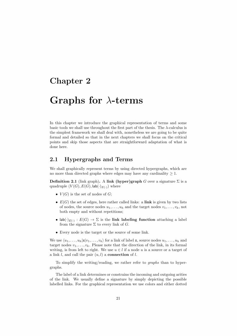
or solid lines (in order to distinguish lines of different colors even when printedout in black and white), but for the time being such details shall simply beomitted, we shall deal with them later on. In this chapter we shall use thefollowing signature Σλ, which contains the links corresponding to the λ-calculusconstructors:

• The variable link:

u

x

v

〈u|v|x〉

The target node x is the sharing node of the link, while its source is anoccurrence of x. While general nodes are usually denoted with u, v, w, . . .we use x, y, z, . . . for sharing nodes, which are meant to represent variables.The idea is that a variable in a term is made out of two components: itsposition in the term, which corresponds to the node u, and its name, givenby x.

• The application link:

u

v w

@

〈u|@|v, w〉

Corresponds to the application constructor of λ-calculus. Its left targetnode is the function node and its right target node is the argumentnode. The @-link is not commutative with respect to its targets, that is,the left and right target will have different, nonexchangeable roles.

• The abstraction link:

v

x u

λ

〈x, v|λ|u〉

One of the two sources of the abstraction link, the one connected to the λthrough a dotted line, is special, and we will need it to be a sharing node.The connection between the λ-link and its sharing node x is the bindingconnection of the λ-link, and x is its variable. The target node is alsocalled the body node of the λ-link.

• The weakening link:

x

w

〈w|x〉

22

We shall need this variation of the variable link to represent, for instance,abstractions like λy.x, whose bound variable has no occurrence in thebody. It is called a weakening, or w-link.

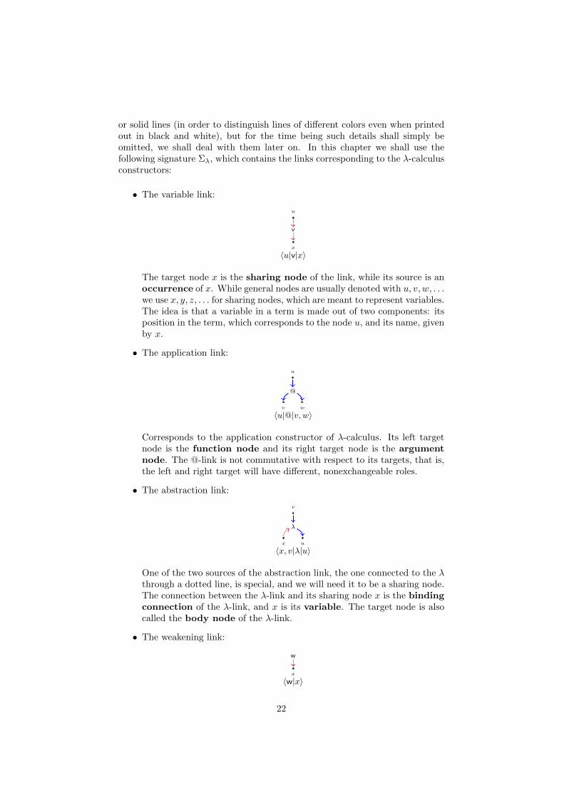
To formally define how terms can be represented through graphs we need tointroduce a few key concepts, which we will do subsequently. First, though, wewould like to present an example of said representation to give the reader anopportunity to familiarize himself with the concept. The following graph is arepresentation of λx.λy.(y (y z)):

u

x

λw

@

@

y z

v v

v

λ

A sharing node x is abstracted if it is the sharing node of a λ-link, it issubstituted if it is the source of a link and is not abstracted, or else it is free(i.e., if it is not the source of a link). In our example x and y are abstracted,while z is free, and there are no substituted sharing nodes.

Nodes which are not the source of any link are the exits of the graph (theonly exit of the example is z), and nodes which are not the target of any link arethe entries of the graph (u). The interface IG of a term graph G is the setof its entries and exits. The interior is the set of nodes inter(G) := V (G) \ IG.

The next section is an informal explanation of how we intend to representterms by graphs.

2.1.1 Sharing and variables

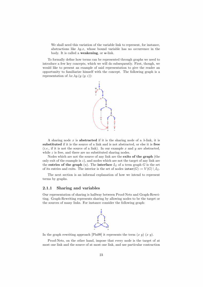
Our representation of sharing is halfway between Proof-Nets and Graph-Rewri-ting. Graph-Rewriting represents sharing by allowing nodes to be the target orthe sources of many links. For instance consider the following graph:

@

x

@

y

@

In the graph rewriting approach [Plu99] it represents the term (x y) (x y).

Proof-Nets, on the other hand, impose that every node is the target of atmost one link and the source of at most one link, and use particular contraction

23

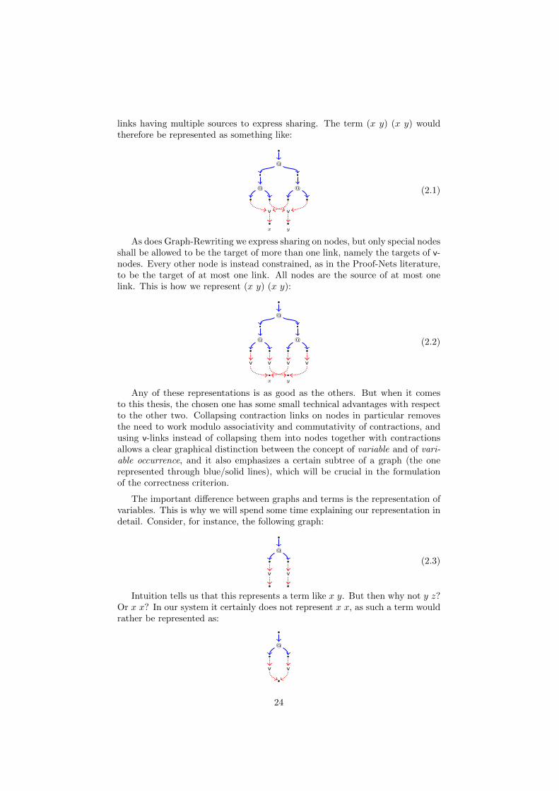
links having multiple sources to express sharing. The term (x y) (x y) wouldtherefore be represented as something like:

@

@ @

x

v

y

v

(2.1)

As does Graph-Rewriting we express sharing on nodes, but only special nodesshall be allowed to be the target of more than one link, namely the targets of v-nodes. Every other node is instead constrained, as in the Proof-Nets literature,to be the target of at most one link. All nodes are the source of at most onelink. This is how we represent (x y) (x y):

@

@ @

x

v v

y

v v

(2.2)

Any of these representations is as good as the others. But when it comesto this thesis, the chosen one has some small technical advantages with respectto the other two. Collapsing contraction links on nodes in particular removesthe need to work modulo associativity and commutativity of contractions, andusing v-links instead of collapsing them into nodes together with contractionsallows a clear graphical distinction between the concept of variable and of vari-able occurrence, and it also emphasizes a certain subtree of a graph (the onerepresented through blue/solid lines), which will be crucial in the formulationof the correctness criterion.

The important difference between graphs and terms is the representation ofvariables. This is why we will spend some time explaining our representation indetail. Consider, for instance, the following graph:

@

v v

(2.3)

Intuition tells us that this represents a term like x y. But then why not y z?Or x x? In our system it certainly does not represent x x, as such a term wouldrather be represented as:

@

v v

24

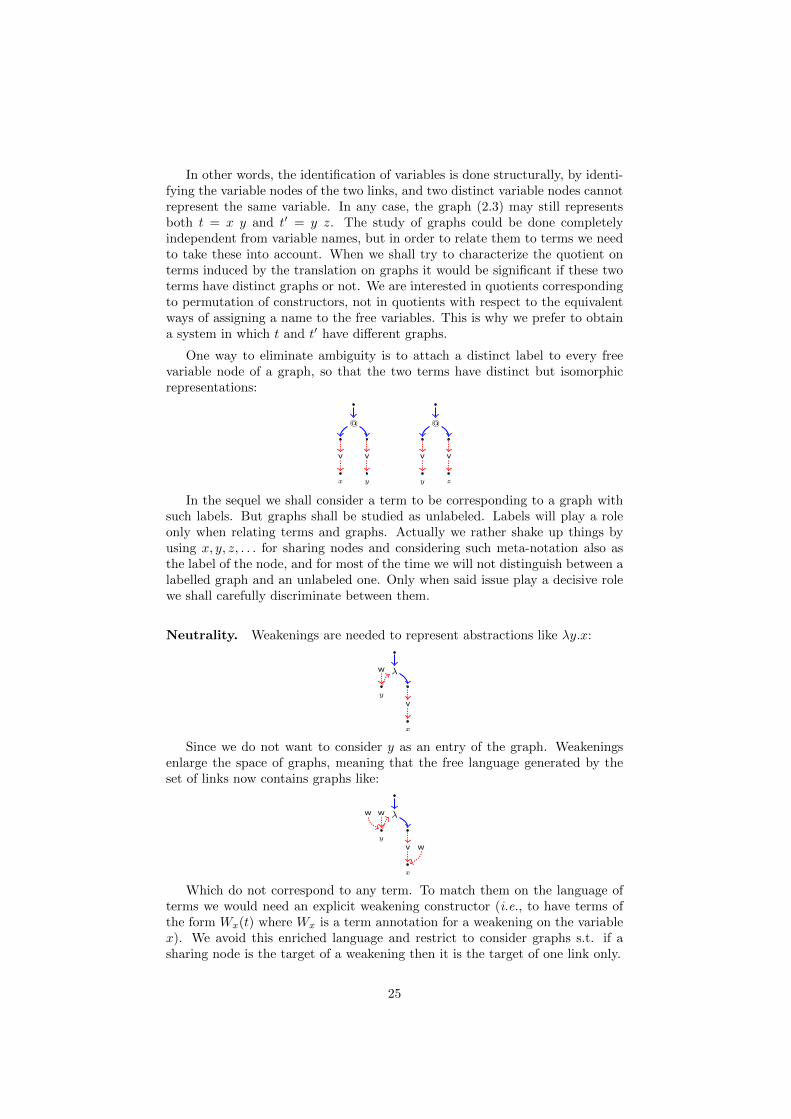
In other words, the identification of variables is done structurally, by identi-fying the variable nodes of the two links, and two distinct variable nodes cannotrepresent the same variable. In any case, the graph (2.3) may still representsboth t = x y and t′ = y z. The study of graphs could be done completelyindependent from variable names, but in order to relate them to terms we needto take these into account. When we shall try to characterize the quotient onterms induced by the translation on graphs it would be significant if these twoterms have distinct graphs or not. We are interested in quotients correspondingto permutation of constructors, not in quotients with respect to the equivalentways of assigning a name to the free variables. This is why we prefer to obtaina system in which t and t′ have different graphs.

One way to eliminate ambiguity is to attach a distinct label to every freevariable node of a graph, so that the two terms have distinct but isomorphicrepresentations:

@

x

v

y

v

@

y

v

z

v

In the sequel we shall consider a term to be corresponding to a graph withsuch labels. But graphs shall be studied as unlabeled. Labels will play a roleonly when relating terms and graphs. Actually we rather shake up things byusing x, y, z, . . . for sharing nodes and considering such meta-notation also asthe label of the node, and for most of the time we will not distinguish between alabelled graph and an unlabeled one. Only when said issue play a decisive rolewe shall carefully discriminate between them.

Neutrality. Weakenings are needed to represent abstractions like λy.x:

y

x

λw

v

Since we do not want to consider y as an entry of the graph. Weakeningsenlarge the space of graphs, meaning that the free language generated by theset of links now contains graphs like:

y

x

λww

v w

Which do not correspond to any term. To match them on the language ofterms we would need an explicit weakening constructor (i.e., to have terms ofthe form Wx(t) where Wx is a term annotation for a weakening on the variablex). We avoid this enriched language and restrict to consider graphs s.t. if asharing node is the target of a weakening then it is the target of one link only.

25

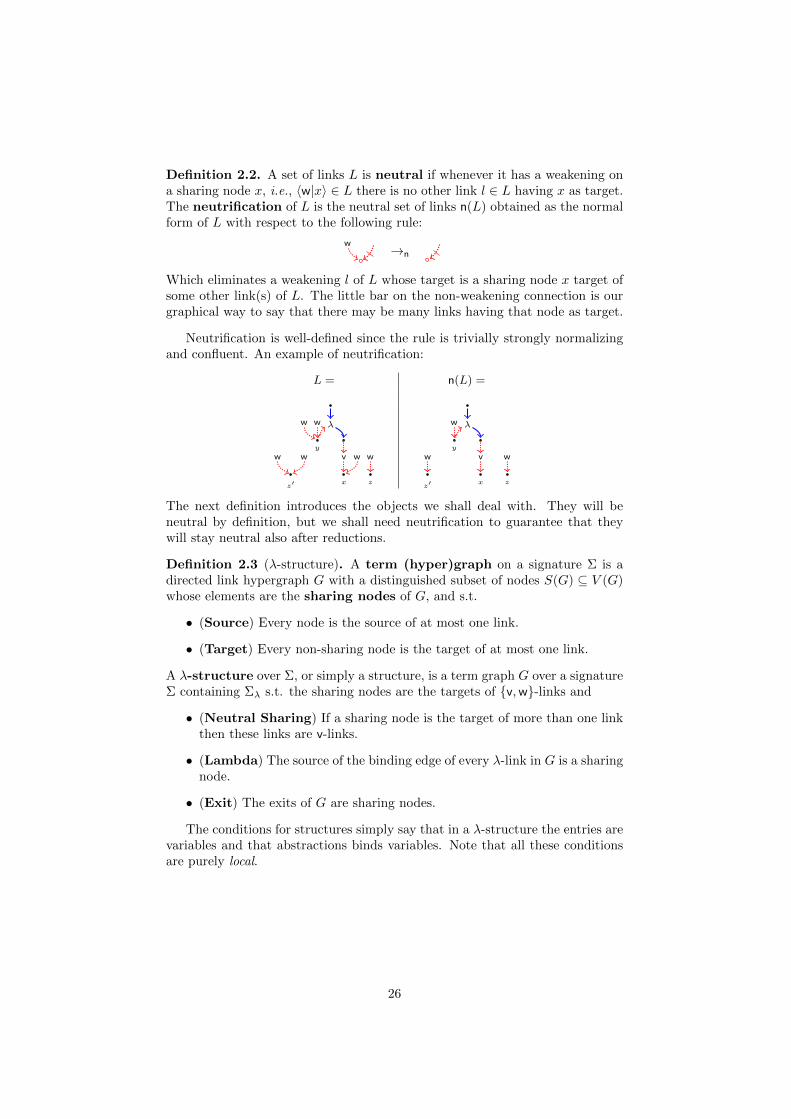
Definition 2.2. A set of links L is neutral if whenever it has a weakening ona sharing node x, i.e., 〈w|x〉 ∈ L there is no other link l ∈ L having x as target.The neutrification of L is the neutral set of links n(L) obtained as the normalform of L with respect to the following rule:

w →n

Which eliminates a weakening l of L whose target is a sharing node x target ofsome other link(s) of L. The little bar on the non-weakening connection is ourgraphical way to say that there may be many links having that node as target.

Neutrification is well-defined since the rule is trivially strongly normalizingand confluent. An example of neutrification:

L = n(L) =

y

x

λww

v w

z

w

z′

wwy

x

λw

v

z

w

z′

w

The next definition introduces the objects we shall deal with. They will beneutral by definition, but we shall need neutrification to guarantee that theywill stay neutral also after reductions.

Definition 2.3 (λ-structure). A term (hyper)graph on a signature Σ is adirected link hypergraph G with a distinguished subset of nodes S(G) ⊆ V (G)whose elements are the sharing nodes of G, and s.t.

• (Source) Every node is the source of at most one link.

• (Target) Every non-sharing node is the target of at most one link.

A λ-structure over Σ, or simply a structure, is a term graph G over a signatureΣ containing Σλ s.t. the sharing nodes are the targets of v,w-links and

• (Neutral Sharing) If a sharing node is the target of more than one linkthen these links are v-links.

• (Lambda) The source of the binding edge of every λ-link in G is a sharingnode.

• (Exit) The exits of G are sharing nodes.

The conditions for structures simply say that in a λ-structure the entries arevariables and that abstractions binds variables. Note that all these conditionsare purely local.

26

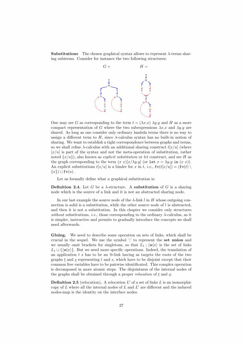
Substitutions The chosen graphical syntax allows to represent λ-terms shar-ing subterms. Consider for instance the two following structures:

G = H =

@

v

λ

v

λ

@

v v

v

λ

One may see G as corresponding to the term t = (λx.x) λy.y and H as a morecompact representation of G where the two subexpressions λx.x and λy.y areshared. As long as one consider only ordinary lambda terms there is no way toassign a different term to H, since λ-calculus syntax has no built-in notion ofsharing. We want to establish a tight correspondence between graphs and terms,so we shall refine λ-calculus with an additional sharing construct t[x/u] (where[x/u] is part of the syntax and not the meta-operation of substitution, rathernoted x/u), also known as explicit substitution or let construct, and see H asthe graph corresponding to the term (x x)[x/λy.y] (or let x = λy.y in (x x)).An explicit substitutions t[x/u] is a binder for x in t, i.e., fv(t[x/u]) = (fv(t) \x) ∪ fv(u).

Let us formally define what a graphical substitution is:

Definition 2.4. Let G be a λ-structure. A substitution of G is a sharingnode which is the source of a link and it is not an abstracted sharing node.

In our last example the source node of the λ-link l in H whose outgoing con-nection is solid is a substitution, while the other source node of l is abstracted,and then it is not a substitution. In this chapter we consider only structureswithout substitutions, i.e., those corresponding to the ordinary λ-calculus, as itis simpler, instructive and permits to gradually introduce the concepts we shallneed afterwards.

Gluing. We need to describe some operation on sets of links, which shall becrucial in the sequel. We use the symbol ’;’ to represent the set union andwe usually omit brackets for singletons, so that L1 ; 〈w|x〉 is the set of linksL1 ∪ 〈w|x〉. But we need more specific operations. Indeed, the translation ofan application t s has to be an @-link having as targets the roots of the twographs t and s representing t and s, which have to be disjoint except that theircommon free variables have to be pairwise identificated. This complex operationis decomposed in more atomic steps. The disjointness of the internal nodes ofthe graphs shall be obtained through a proper relocation of t and s:

Definition 2.5 (relocation). A relocation L′ of a set of links L is an isomorphiccopy of L where all the internal nodes of L and L′ are different and the inducednodes-map is the identity on the interface nodes.

27

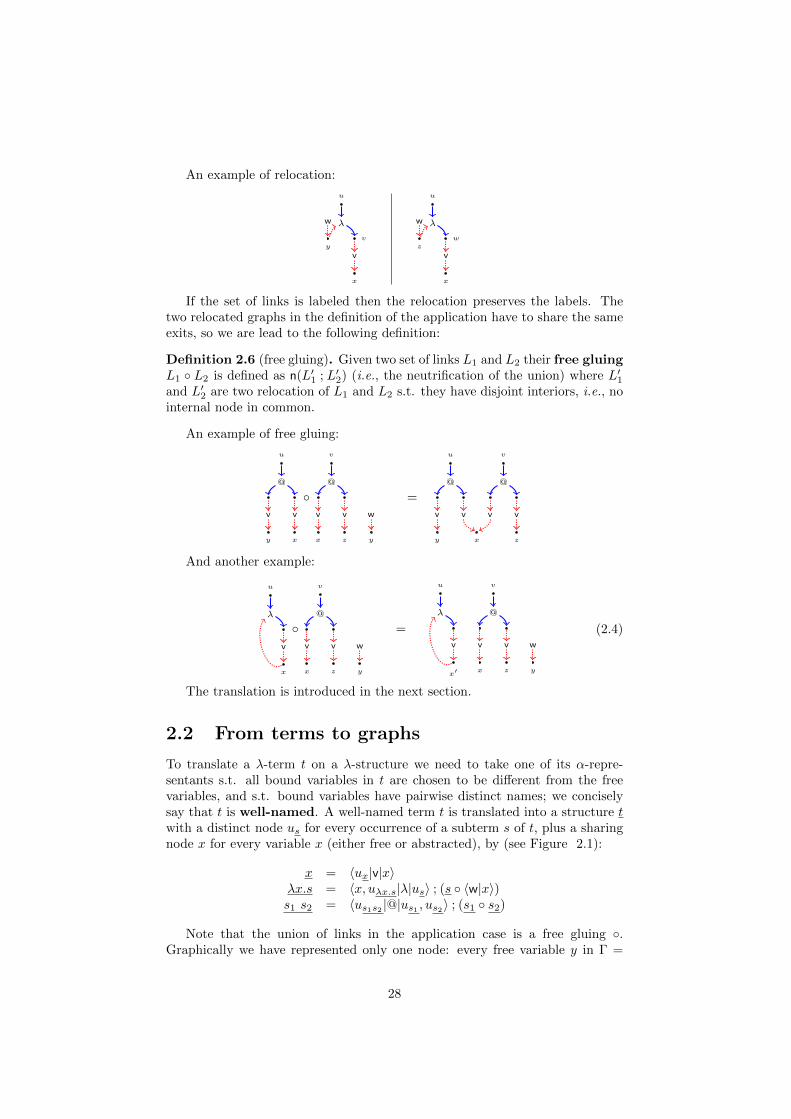
An example of relocation:

u

vy

x

λw

v

u

wz

x

λw

v

If the set of links is labeled then the relocation preserves the labels. Thetwo relocated graphs in the definition of the application have to share the sameexits, so we are lead to the following definition:

Definition 2.6 (free gluing). Given two set of links L1 and L2 their free gluingL1 L2 is defined as n(L′1 ; L′2) (i.e., the neutrification of the union) where L′1and L′2 are two relocation of L1 and L2 s.t. they have disjoint interiors, i.e., nointernal node in common.

An example of free gluing:

u

xy

@

vv

v

zx y

w

@

vv

=

u

xy

@

vv

v

z

@

vv

And another example:

u

x

λ

v

v

zx y

w

@

vv

=

u

x′

λ

v

v

zx

@

vv

y

w

(2.4)

The translation is introduced in the next section.

2.2 From terms to graphs

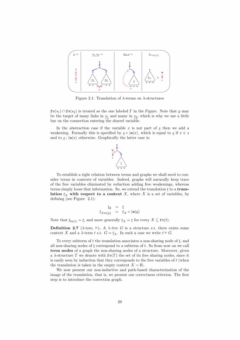
To translate a λ-term t on a λ-structure we need to take one of its α-repre-sentants s.t. all bound variables in t are chosen to be different from the freevariables, and s.t. bound variables have pairwise distinct names; we conciselysay that t is well-named. A well-named term t is translated into a structure twith a distinct node us for every occurrence of a subterm s of t, plus a sharingnode x for every variable x (either free or abstracted), by (see Figure 2.1):

x = 〈ux|v|x〉λx.s = 〈x, uλx.s|λ|us〉 ; (s 〈w|x〉)s1 s2 = 〈us1s2 |@|us1 , us2〉 ; (s1 s2)

Note that the union of links in the application case is a free gluing .Graphically we have represented only one node: every free variable y in Γ =

28

'

&

$

%

x = s1 s2 = λx.s = tY]x

x

v

@

s2s1

Γ

s

x

λ

tY x

w

Figure 2.1: Translation of λ-terms on λ-structures

fv(s1) ∩ fv(s2) is treated as the one labeled Γ in the Figure. Note that y maybe the target of many links in s1 and many in s2, which is why we use a littlebar on the connection entering the shared variable.

In the abstraction case if the variable x is not part of s then we add aweakening. Formally this is specified by s 〈w|x〉, which is equal to s if x ∈ sand to s ; 〈w|x〉 otherwise. Graphically the latter case is:

x

t

λw

To establish a tight relation between terms and graphs we shall need to con-sider terms in contexts of variables. Indeed, graphs will naturally keep traceof the free variables eliminated by reduction adding free weakenings, whereasterms simply loose that information. So, we extend the translation t to a trans-lation tX with respect to a context X, where X is a set of variables, bydefining (see Figure 2.1):

t∅ = ttX]y = tX 〈w|y〉

Note that tfv(t) = t, and more generally tX = t for every X ⊆ fv(t).

Definition 2.7 (λ-tree, ). A λ-tree G is a structure s.t. there exists somecontext X and a λ-term t s.t. G = tX . In such a case we write t G.

To every subterm of t the translation associates a non-sharing node of t, andall non-sharing nodes of t correspond to a subterm of t. So from now on we callterm nodes of a graph the non-sharing nodes of a structure. Moreover, givena λ-structure T we denote with fv(T ) the set of its free sharing nodes, since itis easily seen by induction that they corresponds to the free variables of t (whenthe translation is taken in the empty context X = ∅).

We now present our non-inductive and path-based characterization of theimage of the translation, that is, we present our correctness criterion. The firststep is to introduce the correction graph.

29

'

&

$

%

λ @ vw

⇓(·)∗ ⇓(·)∗ ⇓(·)∗ ⇓(·)∗

Figure 2.2: Correction graph

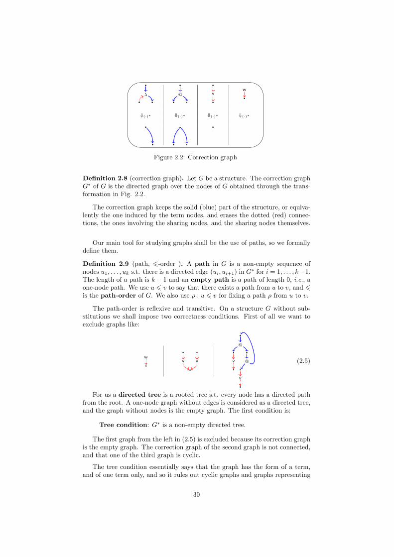
Definition 2.8 (correction graph). Let G be a structure. The correction graphG∗ of G is the directed graph over the nodes of G obtained through the trans-formation in Fig. 2.2.

The correction graph keeps the solid (blue) part of the structure, or equiva-lently the one induced by the term nodes, and erases the dotted (red) connec-tions, the ones involving the sharing nodes, and the sharing nodes themselves.

Our main tool for studying graphs shall be the use of paths, so we formallydefine them.

Definition 2.9 (path, 6-order ). A path in G is a non-empty sequence ofnodes u1, . . . , uk s.t. there is a directed edge (ui, ui+1) in G∗ for i = 1, . . . , k−1.The length of a path is k − 1 and an empty path is a path of length 0, i.e., aone-node path. We use u 6 v to say that there exists a path from u to v, and 6is the path-order of G. We also use ρ : u 6 v for fixing a path ρ from u to v.

The path-order is reflexive and transitive. On a structure G without sub-stitutions we shall impose two correctness conditions. First of all we want toexclude graphs like:

wv v

@

@v

v

(2.5)

For us a directed tree is a rooted tree s.t. every node has a directed pathfrom the root. A one-node graph without edges is considered as a directed tree,and the graph without nodes is the empty graph. The first condition is:

Tree condition: G∗ is a non-empty directed tree.

The first graph from the left in (2.5) is excluded because its correction graphis the empty graph. The correction graph of the second graph is not connected,and that one of the third graph is cyclic.

The tree condition essentially says that the graph has the form of a term,and of one term only, and so it rules out cyclic graphs and graphs representing

30

more than one term. The root of the directed tree shall be referred to as theroot, and noted r. Note that undesired configurations as:

@

vv

Satisfy the tree condition, but they are nonetheless avoided because we re-strict to graphs without substitutions, and so no sharing node can be the sourceof an @-link. This applies more generally to any circular configuration involvingsharing nodes which are not abstracted.

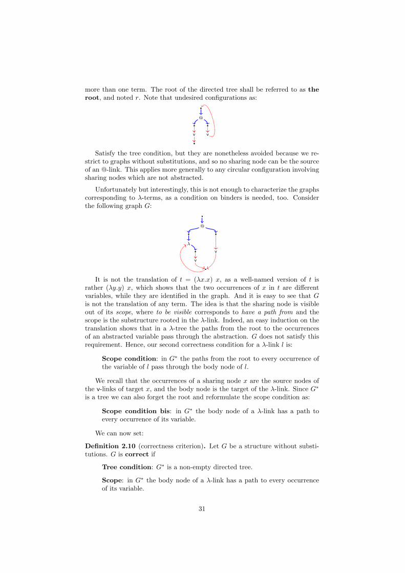
Unfortunately but interestingly, this is not enough to characterize the graphscorresponding to λ-terms, as a condition on binders is needed, too. Considerthe following graph G:

@

λ

v

v

It is not the translation of t = (λx.x) x, as a well-named version of t israther (λy.y) x, which shows that the two occurrences of x in t are differentvariables, while they are identified in the graph. And it is easy to see that Gis not the translation of any term. The idea is that the sharing node is visibleout of its scope, where to be visible corresponds to have a path from and thescope is the substructure rooted in the λ-link. Indeed, an easy induction on thetranslation shows that in a λ-tree the paths from the root to the occurrencesof an abstracted variable pass through the abstraction. G does not satisfy thisrequirement. Hence, our second correctness condition for a λ-link l is:

Scope condition: in G∗ the paths from the root to every occurrence ofthe variable of l pass through the body node of l.

We recall that the occurrences of a sharing node x are the source nodes ofthe v-links of target x, and the body node is the target of the λ-link. Since G∗

is a tree we can also forget the root and reformulate the scope condition as:

Scope condition bis: in G∗ the body node of a λ-link has a path toevery occurrence of its variable.

We can now set:

Definition 2.10 (correctness criterion). Let G be a structure without substi-tutions. G is correct if

Tree condition: G∗ is a non-empty directed tree.

Scope: in G∗ the body node of a λ-link has a path to every occurrenceof its variable.

31

Our correctness criterion is correct, in the following sense:

Lemma 2.11. Let t be a λ-term. Then G = tX is a correct structure withoutsubstitutions whose non-weakening exits are exactly the nodes corresponding tofv(t).

Proof. Straightforward induction on the translation.

The next section shows that the criterion is also complete, i.e., that anycorrect structure without substitutions is a λ-tree.

2.3 From graphs to terms

The completeness of the criterion is proved by extracting from a correct graph Ga term tG s.t. the translation of tG is exactly G. Often this constitutes the proofof the sequentialization theorem, and the extraction procedure, called read-back, is kept implicit, simply described by the proof itself. We prefer to statethe read-back explicitly, prove its properties and obtain the sequentializationtheorem as a corollary, since we shall constantly use the read-back in the nextsections and chapters.

Definition 2.12 (Substructures). Let G be a structure without substitutions.A substructure H of G, noted HCG, is a subset of the links of G which is astructure.

To any term node u it is possible to associate a substructure, the subtreerooted in u.

Definition 2.13 (subtree). Let G be a correct structure without substitutions,u a term node of G. The subtree of u is the minimal set of links G↓u satisfying:

• Base case: if l is a v-link 〈u|v|x〉 then G↓u = l.

• Inductive cases:

– Application: if l = 〈u|@|v, w〉 then G↓u is given by l, G↓v, and G↓w.

– Abstraction: if l = 〈u, x|λ|v〉 then G↓u is given by l, G↓v and theeventual weakening link on x.

Note that the definition is of a local nature. We easily get:

Lemma 2.14. Let G be a correct structure without substitutions and u ∈ G aterm node. Then

1. If u has a path to v in G∗ then v ∈ G↓u and G↓v ⊆ G↓u.

2. G↓u is a correct substructure of G with no free weakening.

Proof. Both points are by induction on the definition of G↓u. The first is im-mediate. If u is the subtree node of a λ-link λ = 〈u, x|λ|v〉 then by i.h. G↓vis correct, and the tree condition for G↓u is obvious. By the scope conditionall occurrences of x, if any, have a path from v. By the first point they, andthe v-links of target x, are in G↓v, so l respects the lambda condition (which isguaranteed by taking the weakening if x has no occurrence) and the scope con-dition, and thus G↓u is correct. The variable case is immediate, the applicationcase follows by the i.h..

32

Remark 2.15. G can be decomposed as G↓r ;W , where r is the root of G and Wis the set of free weakenings of G. Indeed, every link except the weakenings hasa term node, which by the tree condition has a path from r, and the weakeningcompletion for G↓r adds to it all the abstracted weakenings of G.

Subtrees are the first example of implicit box in the thesis.

Now we are ready to define our read-back procedure. A named structure isa structure with a distinct variable label x on every sharing node. We identifythe label and the node.

Definition 2.16 (Read-back). Let G be a named correct structure withoutsubstitutions. The read-back of G is a λ-term G defined recursively on thetree shape of G↓r (where r is the root of G) by the following procedure:

〈r|v|x〉 ;G′ = x

〈r, x|λ|u〉 ;G′ = λx.G↓u〈r|@|u, v〉 ;G′ = G↓u G↓v

Remark 2.17. The read-back is well-defined, as subtrees are correct by lemma2.14 and by acyclicity of G∗ the definition of the read-back is well-founded.

To prove that the translation of the read-back is the graph we started withthe only possible trouble concerns the application case. Indeed, from the defini-tions follows that G↓r = 〈r|@|u, v〉 ; (G↓u ;G↓v) which is almost the translationof an application. We have to be sure that the intersection of G↓u and G↓vcontains sharing nodes of their interfaces only, since in the translation of anapplication G↓u and G↓v are freely glued.

Lemma 2.18 (@-splitting). Let G be a correct structure without substitutionsand whose root link is an @-link l = 〈r|@|u, v〉. Then G↓r = 〈r|@|u, v〉; (G↓u G↓v).

Proof. Suppose that I := G↓u∩G↓v contains a link l with a term node w. Thenby correctness w has a path from v and u. Since there is only one maximal pathν to w, both u and v are on ν and so either u 6 v or v 6 u, but they are sonsof the same node in G∗ and so incomparable with respect to the path order,absurd.If I contains a weakening l then both subtrees contain its binder, which has aterm node, and thus we reduce to the previous case.Suppose that they share a node w which is not an exit node. Then they share theonly link of source w, which is absurd. So the two subtrees are freely glued.

The previous lemma is the analogous of the splitting lemma for Multiplica-tive Proof-Nets, but its proof is much simpler, since we are in an intuitionisticframework and there can only be one concluding @-link, that hence is alwayssplitting. The next step is to prove that the read-back is the inverse of thetranslation, modulo free weakenings:

Proposition 2.19 (the translation is the inverse of the read-back). Let G bea correct structure without substitutions. Then G G, i.e., there exists a set ofvariables X s.t. (G)

X= G. Moreover, if G is connected X = ∅.

33

Actually, for the statement to make sense we should define a notion of equal-ity of λ-trees. We use label-preserving isomorphism as equality, but the isomor-phism will never be used explicitly.

Proof. By induction on the number k of links in G. Suppose k = 1 and let lbe the only link. By the exit and lambda condition for λ-structures l is a v-link〈u|v|x〉. Then G = x and (G)

∅= G.

Suppose k > 1. If there is a free weakening l = 〈w|y〉 then by i.h. there existsX s.t. (G \ l)

X= G \ l. Then (G)

X∪y= G. Otherwise there are no free

weakenings and if the output link is

• An abstraction: then G = 〈r, y|λ|v〉 ; G′, where G′ = 〈w|y〉 G↓v. G′

is correct so by i.h. there exists X s.t. (G′)X

= G′, and we know that

we can take X = y, since in G↓v there are no free weakenings. Then(G)∅

= (λy.G′)∅

= 〈r, y|λ|v〉 ; (G′)y

= G.

• An application: then by the @-splitting lemma G = 〈r|@|u, v〉;(G↓uG↓v).By i.h. we get (G↓u)

∅= G↓u and (G↓v)∅ = G↓v. We conclude as (G)

∅=

(G↓u G↓v)∅ = 〈r|@|u, v〉 ; ((G↓u)∅ (G↓v)∅) =i.h. G.

It is easy to see that there is a unique set of variables X s.t. fv(G) ∩X =∅ and satisfying (G)

X= G. The previous result can be rephrased into the

traditional statement:

Corollary 2.20 (Sequentialization). Let G be a structure without substitutions.G is a λ-tree iff it is correct.

Proof. ⇒) Lemma 2.11. ⇐) Proposition 2.19.

We defined substructures and focused in particular on some of them, thesubtrees. When a structure G is correct then its subtrees are correct. Are thereany other correct substructures? Can we say something about them? Can weobtain different read-backs?

We can prove that subtrees are the only correct substructures of a correctstructure, modulo weakenings.

Theorem 2.21 (unique box). Let G be a correct structure without substitutionsand u ∈ G a term node of G. G↓u is the unique connected correct substructureof G of root u.

Proof. Let H be a connected substructure of G of root u. We show H ⊆ G↓uand G↓u ⊆ H. First of all note that by connectedness the weakenings are inbijection with, and attached to, the λ-links, so if the two structures have thesame λ-links they have the same weakenings.H ⊆ G↓u) If l is a @, λ, v-link in H then by the tree condition the source termnode of l has a path from u in H, thus in G and so by lemma 2.14 l belongs toG↓u.G↓u ⊆ H) Let L be the set of @, λ, v-links of G↓u which are not in H, andchose l among the links in L so that the source term node v of l is at minimaldistance from u in G∗. By minimality of l we get v ∈ H and that v is an exit

34

of H, thus a sharing node, which implies that G↓u has a substitution, absurd.Hence, L = ∅ and G↓u ⊆ H.

One of the reasons for considering graphical representations of terms orproofs is that often the translation maps different terms to the same graph. Itis interesting to characterize the equivalence relation induced by the translation,since it can generally be considered as an operational equivalence. We concludethis section by proving that the translation we showed is injective, i.e., it doesnot quotient the set of terms.

For the following lemma we consider literal equality of λ-terms, and notequality modulo α-conversion. Moreover, T is considered as a named λ-tree.

Lemma 2.22 (graphical quotient). Let t, s be well-named λ-terms. If t Tand s T then t = s.

Proof. If tX = sY has a free weakening of variable z then z ∈ X and z ∈ Y ,and we conclude using the i.h.. So we can assume tX = sY connected and thusX = Y = ∅. We show t = u by induction on the number of links of t, which isa λ-tree T without isolated weakenings. Consider the root link l of t:

• If l is a v-link 〈u|v|x〉 then necessarily t = s = x.

• If l is an abstraction then there exist t′ and s′ s.t. t = λx.t′ and s = λy.s′,as only terms of the shape λx.M are translated to graphs with a rootλ-link. The variable node of l is labeled, since T is considered as a namedλ-tree, and so we get x = y, because the outermost abstraction of t andthat one of s are both mapped on l. Let G′ be G without l, and if thevariable of l is a weakening i then also without i. G′ is connected andG = t′ = s′. By i.h. we get t′ = s′, and so t = λx.t′ = λx.s′ = s.

• If l is an application then by the definition of the translation it can onlybe that t = t1 t2 and s = s1 s2 with t1 = s1 and t2 = s2. By i.h. we gett1 = s1 and t2 = s2, and so t = s.

Remark 2.23. As we said before the notion of equality we consider for graphsis label-preserving (hyper)graph-isomorphism. It is easy to see that two λ-terms are α-equivalent if and only if their corresponding λ-trees are related bya graph-isomorphism which preserves the labels of exit nodes only. Taking asgraph equality plain graph-isomorphism corresponds on terms to an extensionof α-equivalence which relates terms differing for injective renamings of freevariables too, where an injective renaming is a renaming that sends distinctnames on distinct names. Conceptually, it is not hard to refine lemma 2.22in order to relate α-equivalence classes of terms and λ-trees, but technicallyit requires some care. For λ-trees this can be done, but in later chapters thecharacterization of the quotients induced by translations will already be quitetechnical so that to simplify them we shall avoid such details and work withliteral equality on terms and named graphs, as we did here.

Proposition 2.19 proved that if G = t then t G, i.e., that the translationwith respect to a context is the inverse of the read-back. We have now provedthat the read-back is the inverse of , too.

35

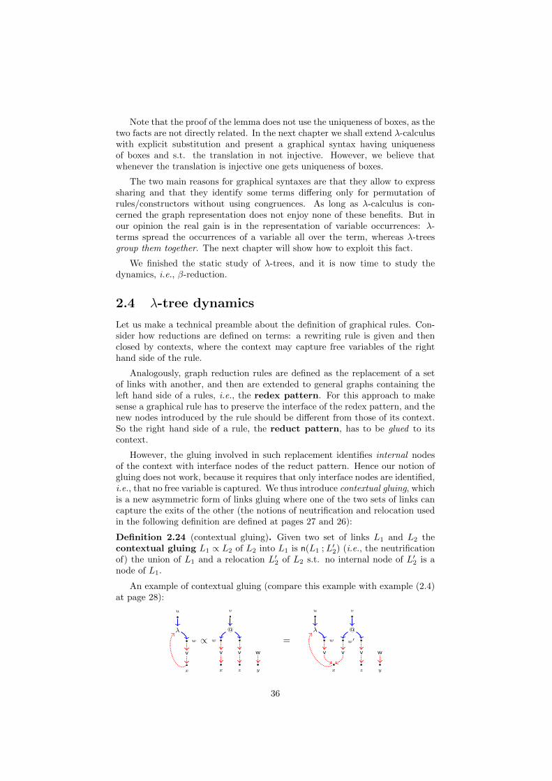
Note that the proof of the lemma does not use the uniqueness of boxes, as thetwo facts are not directly related. In the next chapter we shall extend λ-calculuswith explicit substitution and present a graphical syntax having uniquenessof boxes and s.t. the translation in not injective. However, we believe thatwhenever the translation is injective one gets uniqueness of boxes.

The two main reasons for graphical syntaxes are that they allow to expresssharing and that they identify some terms differing only for permutation ofrules/constructors without using congruences. As long as λ-calculus is con-cerned the graph representation does not enjoy none of these benefits. But inour opinion the real gain is in the representation of variable occurrences: λ-terms spread the occurrences of a variable all over the term, whereas λ-treesgroup them together. The next chapter will show how to exploit this fact.

We finished the static study of λ-trees, and it is now time to study thedynamics, i.e., β-reduction.

2.4 λ-tree dynamics

Let us make a technical preamble about the definition of graphical rules. Con-sider how reductions are defined on terms: a rewriting rule is given and thenclosed by contexts, where the context may capture free variables of the righthand side of the rule.

Analogously, graph reduction rules are defined as the replacement of a setof links with another, and then are extended to general graphs containing theleft hand side of a rules, i.e., the redex pattern. For this approach to makesense a graphical rule has to preserve the interface of the redex pattern, and thenew nodes introduced by the rule should be different from those of its context.So the right hand side of a rule, the reduct pattern, has to be glued to itscontext.

However, the gluing involved in such replacement identifies internal nodesof the context with interface nodes of the reduct pattern. Hence our notion ofgluing does not work, because it requires that only interface nodes are identified,i.e., that no free variable is captured. We thus introduce contextual gluing, whichis a new asymmetric form of links gluing where one of the two sets of links cancapture the exits of the other (the notions of neutrification and relocation usedin the following definition are defined at pages 27 and 26):

Definition 2.24 (contextual gluing). Given two set of links L1 and L2 thecontextual gluing L1 ∝ L2 of L2 into L1 is n(L1 ; L′2) (i.e., the neutrificationof) the union of L1 and a relocation L′2 of L2 s.t. no internal node of L′2 is anode of L1.

An example of contextual gluing (compare this example with example (2.4)at page 28):

u

w

x

λ

v

∝

v

w

zx y

w

@

vv

=

u

w

x

λ

v

v

z

w′

@

vv

y

w

36

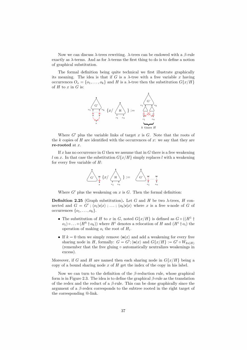
Now we can discuss λ-trees rewriting. λ-trees can be endowed with a β-ruleexactly as λ-terms. And as for λ-terms the first thing to do is to define a notionof graphical substitution.

The formal definition being quite technical we first illustrate graphicallyits meaning. The idea is that if G is a λ-tree with a free variable x havingoccurrences Ox = o1, . . . , ok and H is a λ-tree then the substitution Gx/Hof H to x in G is:

G’

o1 ok. . .

x

v v

x/ H

z1 zn

. . .

:=

G’

o1 ok. . .

z1 zn

k times H

Where G′ plus the variable links of target x is G. Note that the roots ofthe k copies of H are identified with the occurrences of x: we say that they arere-rooted at x.

If x has no occurrence inG then we assume that inG there is a free weakeningl on x. In that case the substitution Gx/H simply replaces l with a weakeningfor every free variable of H:

G’

x

w x/ H

z1 zn

. . .

:= G’

z1

w

zn

w. . .

Where G′ plus the weakening on x is G. Then the formal definition:

Definition 2.25 (Graph substitution). Let G and H be two λ-trees, H con-nected and G = G′ ; 〈o1|v|x〉 ; . . . ; 〈ok|v|x〉 where x is a free v-node of G ofoccurrences o1, . . . , ok.

• The substitution of H to x in G, noted Gx/H is defined as G ((H1 †o1) . . . (Hk † ok)) where Hi denotes a relocation of H and (Hi † oi) theoperation of making oi the root of Hi.

• If k = 0 then we simply remove 〈w|x〉 and add a weakening for every freesharing node in H, formally: G = G′; 〈w|x〉 and Gx/H := G′ Wfv(H)

(remember that the free gluing automatically neutralizes weakenings inexcess).

Moreover, if G and H are named then each sharing node in Gx/H being acopy of a bound sharing node x of H get the index of the copy in his label.

Now we can turn to the definition of the β-reduction rule, whose graphicalform is in Figure 2.3. The idea is to define the graphical β-rule as the translationof the redex and the reduct of a β-rule. This can be done graphically since theargument of a β-redex corresponds to the subtree rooted in the right target ofthe corresponding @-link.

37

'

&

$

%

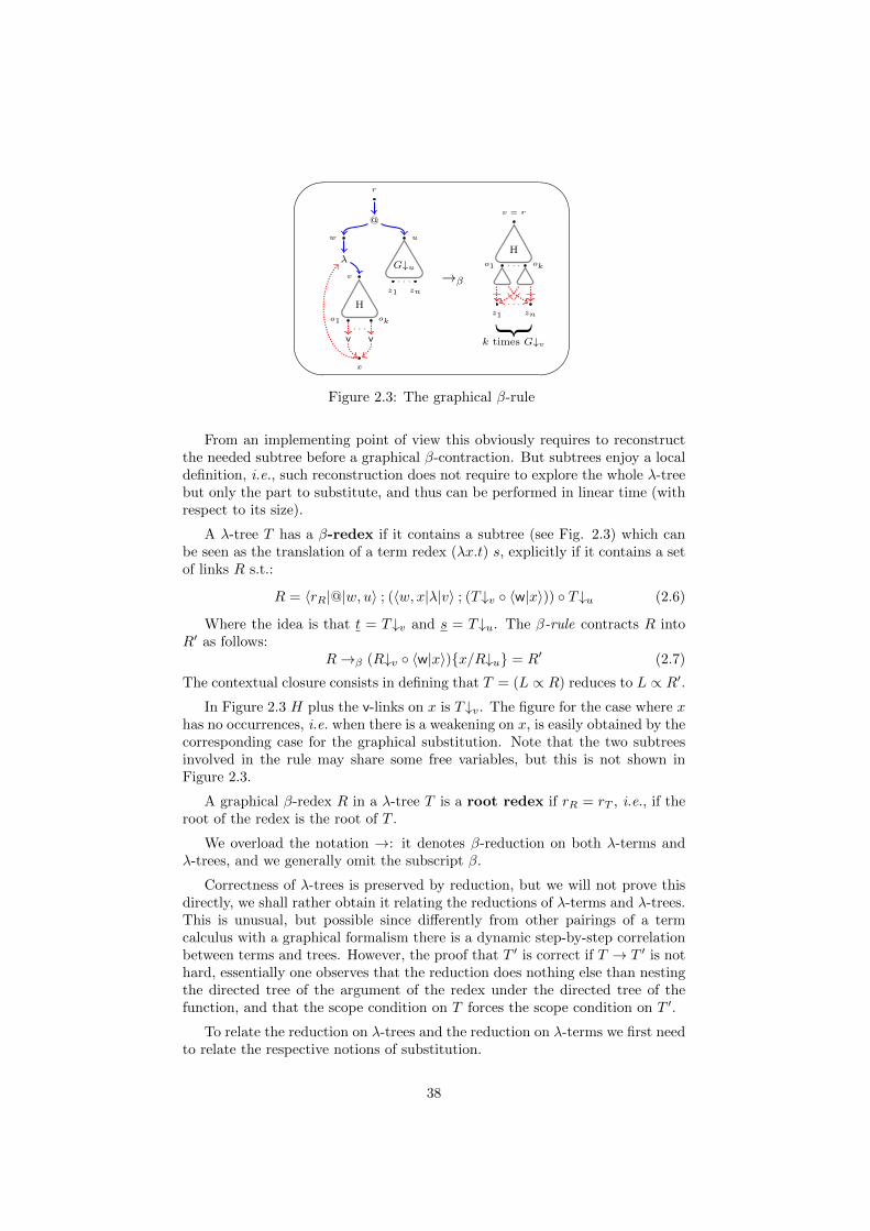
r

w u

@

G↓u

z1 zn

. . .v

H

o1 ok. . .

x

v v

λ

→β

v = r

H

o1 ok. . .

z1 znk times G↓v

. . .

Figure 2.3: The graphical β-rule

From an implementing point of view this obviously requires to reconstructthe needed subtree before a graphical β-contraction. But subtrees enjoy a localdefinition, i.e., such reconstruction does not require to explore the whole λ-treebut only the part to substitute, and thus can be performed in linear time (withrespect to its size).

A λ-tree T has a β-redex if it contains a subtree (see Fig. 2.3) which canbe seen as the translation of a term redex (λx.t) s, explicitly if it contains a setof links R s.t.:

R = 〈rR|@|w, u〉 ; (〈w, x|λ|v〉 ; (T↓v 〈w|x〉)) T↓u (2.6)

Where the idea is that t = T↓v and s = T↓u. The β-rule contracts R intoR′ as follows:

R→β (R↓v 〈w|x〉)x/R↓u = R′ (2.7)

The contextual closure consists in defining that T = (L ∝ R) reduces to L ∝ R′.In Figure 2.3 H plus the v-links on x is T↓v. The figure for the case where x

has no occurrences, i.e. when there is a weakening on x, is easily obtained by thecorresponding case for the graphical substitution. Note that the two subtreesinvolved in the rule may share some free variables, but this is not shown inFigure 2.3.

A graphical β-redex R in a λ-tree T is a root redex if rR = rT , i.e., if theroot of the redex is the root of T .

We overload the notation →: it denotes β-reduction on both λ-terms andλ-trees, and we generally omit the subscript β.

Correctness of λ-trees is preserved by reduction, but we will not prove thisdirectly, we shall rather obtain it relating the reductions of λ-terms and λ-trees.This is unusual, but possible since differently from other pairings of a termcalculus with a graphical formalism there is a dynamic step-by-step correlationbetween terms and trees. However, the proof that T ′ is correct if T → T ′ is nothard, essentially one observes that the reduction does nothing else than nestingthe directed tree of the argument of the redex under the directed tree of thefunction, and that the scope condition on T forces the scope condition on T ′.

To relate the reduction on λ-trees and the reduction on λ-terms we first needto relate the respective notions of substitution.

38

Lemma 2.26. Let G = tX and H = u two λ-trees and z ∈ X. Thentz/u

(X∪fv(u))\z= Gz/H, and so in particular Gz/H is correct.

Proof. Easy induction on t.

We can now prove the exact relation between λ-terms and λ-trees.

Theorem 2.27 (dynamic relation). Let t be a λ-term and T a λ-tree s.t. t T .

1. If t→ t′ then there exists a unique λ-tree T ′ s.t. T → T ′ and t′ T ′, andconversely:

2. If T → T ′ then there exists a unique term t′ s.t. t→ t′ and t′ T ′.

Proof. By induction on , i.e., by induction on the translation. Suppose t T .The only interesting case is if t is an application M N . Then there exists aset of variables X s.t. tX = (〈r|@|u, v〉 ; M N) WX = T , where T↓u = Mand T↓v = N by definition of read-back and proposition 2.19, i.e., M T↓uand N T↓v. Let M → M ′, then by the i.h. M → T ′′ with M ′ T ′′. Theλ-tree T ′′ writes as T ′′′ ;WY , where WY is the set of free weakenings of T ′′ andM ′ T ′′′. Then t→M ′ N and

tX → (〈r|@|u, v〉 ;T ′′ N) WX = (〈r|@|u, v〉 ;T ′′′ N) WX WY = M ′ NX∪Y

Now let T ′ = M ′ NX∪Y and suppose that there is another λ-tree T0 satisfyingthe statement. From M ′ N T0 and definition of it follows that T0 and T ′

can only differ in the number of free weakenings. But the reduction of the redexin tX is deterministic so that there is only one set of weakenings satisfying thestatement, hence T ′ = T0. Conversely, by lemma 2.22 given T ′ there is only oneterm which translates to t′ so that t′ is unique.If there is a redex in M , in N or in N the proof proceeds analogously.The only eventual redex of t that cannot be contained in N or M is the onegiven by the application of M and N if M = λy.s. By translation and read-backt has such a redex if and only if T has a root redex too, and T cannot have anyother redex R′ , since if the root rR′ is not r then it has a path to either u or vand then R′ is contained either in T↓u = M or T↓v = N .The reduct of this outermost is t→ sy/N. By definition:

T = tX = (〈rR|@|w, uN 〉 ; ((〈w, x|λ|us〉 ; sy) N)) WX

Where T↓us = s and T↓uN = N by definition of read-back and proposition 2.19.Then T = tX reduces to

T ′ = (sy)y/N WX = sy∪Xy/N

Which by the substitution lemma is sy/N(X∪fv(N))\y

, and so t′ = sy/N T ′. Unicity is obtained as before, and we conclude.

The theorem states that is a strong bisimulation.

Definition 2.28 (strong bisimulation). Let (S,→) and (Q, ) two rewritingsystems, with reduction steps labelled from a common set L. A strong bisim-ulation between S and Q is a relation ≡ between terms of S and terms of Qs.t. if s ≡ q, with s ∈ S and q ∈ Q, then for a ∈ L:

39

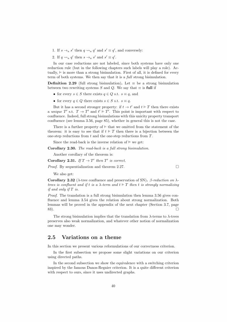
1. If s→a s′ then q a q

′ and s′ ≡ q′, and conversely:

2. If q a q′ then s→a s

′ and s′ ≡ q′.In our case reductions are not labeled, since both systems have only one

reduction rule (but in the following chapters such labels will play a role). Ac-tually, is more than a strong bisimulation. First of all, it is defined for everyterm of both systems. We then say that it is a full strong bisimulation.

Definition 2.29 (full strong bisimulation). Let ≡ be a strong bisimulationbetween two rewriting systems S and Q. We say that ≡ is full if

• for every s ∈ S there exists q ∈ Q s.t. s ≡ q, and

• for every q ∈ Q there exists s ∈ S s.t. s ≡ q.But it has a second stronger property: if t→ t′ and t T then there exists

a unique T ′ s.t. T → T ′ and t′ T ′. This point is important with respect toconfluence. Indeed, full strong bisimulations with this unicity property transportconfluence (see lemma 3.56, page 85), whether in general this is not the case.

There is a further property of that we omitted from the statement of thetheorem: it is easy to see that if t T then there is a bijection between theone-step reductions from t and the one-step reductions from T .

Since the read-back is the inverse relation of we get:

Corollary 2.30. The read-back is a full strong bisimulation.

Another corollary of the theorem is:

Corollary 2.31. If T → T ′ then T ′ is correct.

Proof. By sequentialization and theorem 2.27.

We also get:

Corollary 2.32 (λ-tree confluence and preservation of SN). β-reduction on λ-trees is confluent and if t is a λ-term and t T then t is strongly normalizingif and only if T is.

Proof. The translation is a full strong bisimulation then lemma 3.56 gives con-fluence and lemma 3.54 gives the relation about strong normalization. Bothlemmas will be proved in the appendix of the next chapter (Section 3.7, page83).

The strong bisimulation implies that the translation from λ-terms to λ-treespreserves also weak normalization, and whatever other notion of normalizationone may wonder.

2.5 Variations on a theme

In this section we present various reformulations of our correctness criterion.

In the first subsection we propose some slight variations on our criterionusing directed paths.

In the second subsection we show the equivalence with a switching criterioninspired by the famous Danos-Regnier criterion. It is a quite different criterionwith respect to ours, since it uses undirected graphs.

40

'

&

$

%

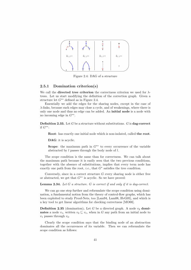
λ @ vw

⇓(·)∗∗ ⇓(·)∗∗ ⇓(·)∗∗ ⇓(·)∗∗

Figure 2.4: DAG of a structure

2.5.1 Domination criterion(s)

We call the directed tree criterion the correctness criterion we used for λ-trees. Let us start modifying the definition of the correction graph. Given astructure let G∗∗ defined as in Figure 2.4.

Essentially we add the edges for the sharing nodes, except in the case ofλ-links, because such edges may close a cycle, and of weakenings, where there isonly one node and thus no edge can be added. An initial node is a node withno incoming edge in G∗∗.

Definition 2.33. Let G be a structure without substitutions. G is dag-correctif G∗∗:

Root: has exactly one initial node which is non-isolated, called the root.

DAG: it is acyclic.

Scope: the maximum path in G∗∗ to every occurrence of the variableabstracted by l passes through the body node of l.

The scope condition is the same than for correctness. We can talk aboutthe maximum path because it is easily seen that the two previous conditions,together with the absence of substitutions, implies that every term node hasexactly one path from the root, i.e., that G∗ satisfies the tree condition.

Conversely, since in a correct structure G every sharing node is either freeor abstracted, we get that G∗∗ is acyclic. So we have proved:

Lemma 2.34. Let G a structure. G is correct if and only if it is dag-correct.

We can go one step further and reformulate the scope condition using domi-nation, a fundamental notion from the theory of control-flow graphs, which hasbeen exploited to study Proof-Nets, too [Lam94, Lam08, HvG05], and which isa key tool to get linear algorithms for checking correctness [MO00].

Definition 2.35 (domination). Let G be a directed graph. A node v2 domi-nates a node v1, written v2 v v1, when in G any path from an initial node tov1 passes through v2.

Clearly the scope condition says that the binding node of an abstractiondominates all the occurrences of its variable. Then we can reformulate thescope condition as follows:

41

Domination Scope: the binding node of every abstraction l dominatesits variable, whenever it is not the node of a weakening.

It is immediate that the scope and the domination scope conditions areequivalent. So if we call domination-correct a structure satisfying the root,DAG and domination scope condition we get:

Lemma 2.36. Let G a structure. G is correct if and only if it is domination-correct.

Let us give a fourth equivalent formulation of the scope condition, based onconnectedness:

Connecting Scope: for every abstraction l whose variable is not a weak-ening the removal of the binding node of l from G∗∗ disconnects its variablefrom the root.

Once again it is immediate that in presence of the root and DAG conditionthe connecting scope condition is equivalent to the domination one. Formulatedthis way the condition is not independent from the root condition, but we canrephrase it by asking that the variable is disconnected from the source termnode of the λ-link, which by the root and DAG condition has a path from theroot.

The connecting scope formulation can also be used with the tree condition.There one can also rephrase it without reference to any other node, askingthat the removal creates as many new connected components as the number ofoccurrences of the variable.

Let us come back to the domination scope condition. The exception aboutthe weakening is due to the fact that in that case there is no path from thebinding node of a λ-link to its variable, and so domination does not hold (sincethe weakening node itself is an initial node with an empty path to itself).

To overcome that exception either one tries to change the notion of domina-tion, or to add some edges to G∗∗. The second choice seems more reasonable,as domination is a very natural notion. The idea is to modify the case aboutthe λ-link in the definition of G∗∗.

At first sight the only possibility is to use the following pattern:

λ ⇒

Since orienting the new edge in the opposite direction would introduce cyclesin the case of non-weakening variables. Then we can use the following condition:

Domination Scope bis: the binding node of every abstraction l domi-nates its variable.

Which is the domination condition without the side condition. The two areclearly equivalent.

42

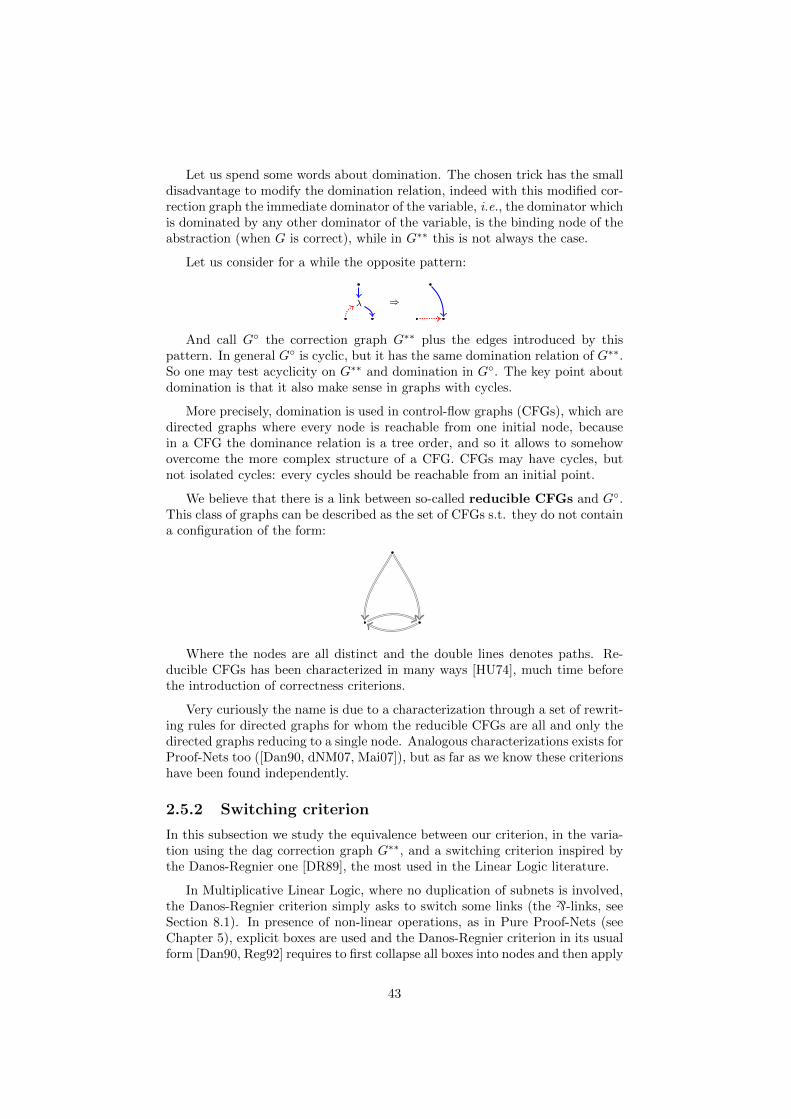
Let us spend some words about domination. The chosen trick has the smalldisadvantage to modify the domination relation, indeed with this modified cor-rection graph the immediate dominator of the variable, i.e., the dominator whichis dominated by any other dominator of the variable, is the binding node of theabstraction (when G is correct), while in G∗∗ this is not always the case.

Let us consider for a while the opposite pattern:

λ ⇒

And call G the correction graph G∗∗ plus the edges introduced by thispattern. In general G is cyclic, but it has the same domination relation of G∗∗.So one may test acyclicity on G∗∗ and domination in G. The key point aboutdomination is that it also make sense in graphs with cycles.

More precisely, domination is used in control-flow graphs (CFGs), which aredirected graphs where every node is reachable from one initial node, becausein a CFG the dominance relation is a tree order, and so it allows to somehowovercome the more complex structure of a CFG. CFGs may have cycles, butnot isolated cycles: every cycles should be reachable from an initial point.

We believe that there is a link between so-called reducible CFGs and G.This class of graphs can be described as the set of CFGs s.t. they do not containa configuration of the form:

Where the nodes are all distinct and the double lines denotes paths. Re-ducible CFGs has been characterized in many ways [HU74], much time beforethe introduction of correctness criterions.

Very curiously the name is due to a characterization through a set of rewrit-ing rules for directed graphs for whom the reducible CFGs are all and only thedirected graphs reducing to a single node. Analogous characterizations exists forProof-Nets too ([Dan90, dNM07, Mai07]), but as far as we know these criterionshave been found independently.

2.5.2 Switching criterion

In this subsection we study the equivalence between our criterion, in the varia-tion using the dag correction graph G∗∗, and a switching criterion inspired bythe Danos-Regnier one [DR89], the most used in the Linear Logic literature.

In Multiplicative Linear Logic, where no duplication of subnets is involved,the Danos-Regnier criterion simply asks to switch some links (the `-links, seeSection 8.1). In presence of non-linear operations, as in Pure Proof-Nets (seeChapter 5), explicit boxes are used and the Danos-Regnier criterion in its usualform [Dan90, Reg92] requires to first collapse all boxes into nodes and then apply

43

#

"

!

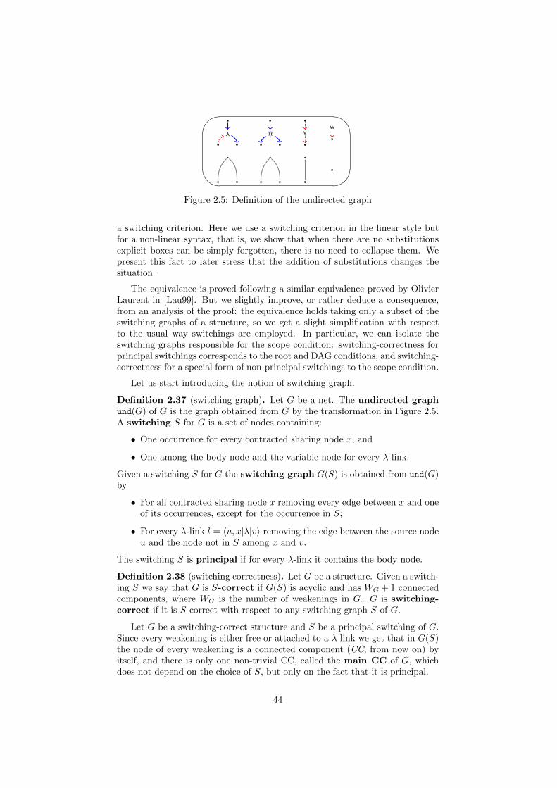
λ @ vw

Figure 2.5: Definition of the undirected graph

a switching criterion. Here we use a switching criterion in the linear style butfor a non-linear syntax, that is, we show that when there are no substitutionsexplicit boxes can be simply forgotten, there is no need to collapse them. Wepresent this fact to later stress that the addition of substitutions changes thesituation.

The equivalence is proved following a similar equivalence proved by OlivierLaurent in [Lau99]. But we slightly improve, or rather deduce a consequence,from an analysis of the proof: the equivalence holds taking only a subset of theswitching graphs of a structure, so we get a slight simplification with respectto the usual way switchings are employed. In particular, we can isolate theswitching graphs responsible for the scope condition: switching-correctness forprincipal switchings corresponds to the root and DAG conditions, and switching-correctness for a special form of non-principal switchings to the scope condition.

Let us start introducing the notion of switching graph.

Definition 2.37 (switching graph). Let G be a net. The undirected graphund(G) of G is the graph obtained from G by the transformation in Figure 2.5.A switching S for G is a set of nodes containing:

• One occurrence for every contracted sharing node x, and

• One among the body node and the variable node for every λ-link.

Given a switching S for G the switching graph G(S) is obtained from und(G)by

• For all contracted sharing node x removing every edge between x and oneof its occurrences, except for the occurrence in S;

• For every λ-link l = 〈u, x|λ|v〉 removing the edge between the source nodeu and the node not in S among x and v.

The switching S is principal if for every λ-link it contains the body node.

Definition 2.38 (switching correctness). Let G be a structure. Given a switch-ing S we say that G is S-correct if G(S) is acyclic and has WG + 1 connectedcomponents, where WG is the number of weakenings in G. G is switching-correct if it is S-correct with respect to any switching graph S of G.

Let G be a switching-correct structure and S be a principal switching of G.Since every weakening is either free or attached to a λ-link we get that in G(S)the node of every weakening is a connected component (CC, from now on) byitself, and there is only one non-trivial CC, called the main CC of G, whichdoes not depend on the choice of S, but only on the fact that it is principal.

44

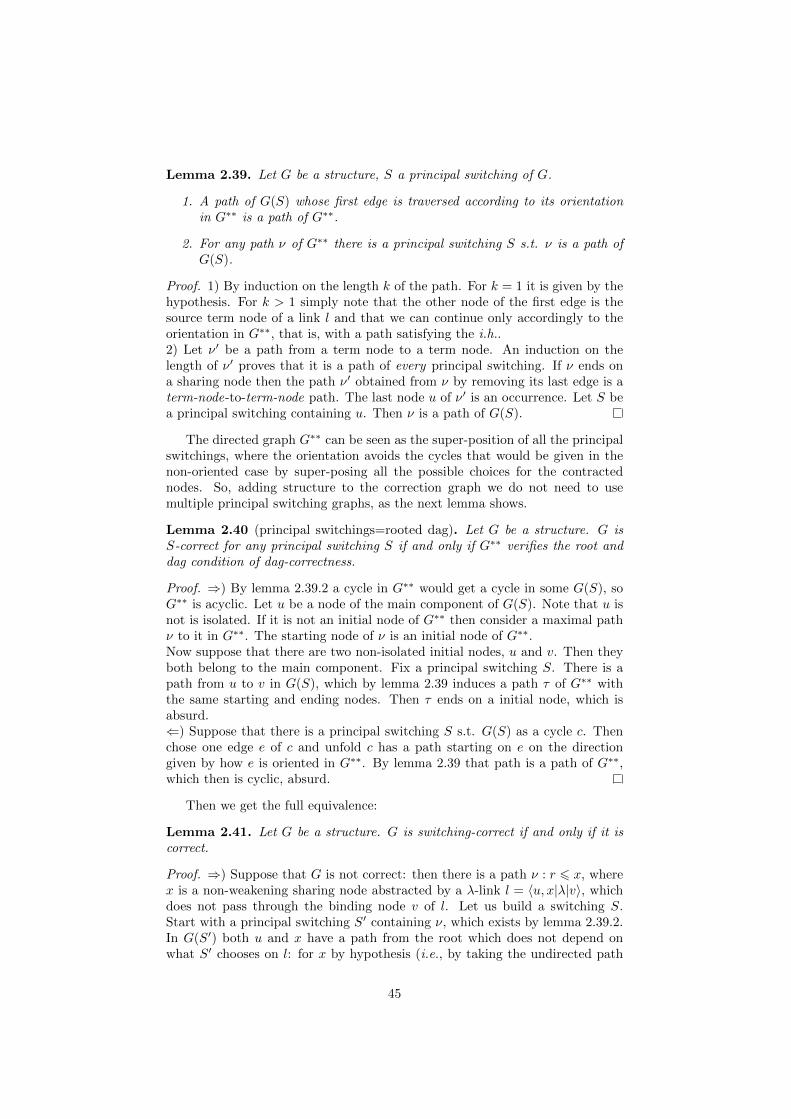
Lemma 2.39. Let G be a structure, S a principal switching of G.

1. A path of G(S) whose first edge is traversed according to its orientationin G∗∗ is a path of G∗∗.

2. For any path ν of G∗∗ there is a principal switching S s.t. ν is a path ofG(S).

Proof. 1) By induction on the length k of the path. For k = 1 it is given by thehypothesis. For k > 1 simply note that the other node of the first edge is thesource term node of a link l and that we can continue only accordingly to theorientation in G∗∗, that is, with a path satisfying the i.h..2) Let ν′ be a path from a term node to a term node. An induction on thelength of ν′ proves that it is a path of every principal switching. If ν ends ona sharing node then the path ν′ obtained from ν by removing its last edge is aterm-node-to-term-node path. The last node u of ν′ is an occurrence. Let S bea principal switching containing u. Then ν is a path of G(S).

The directed graph G∗∗ can be seen as the super-position of all the principalswitchings, where the orientation avoids the cycles that would be given in thenon-oriented case by super-posing all the possible choices for the contractednodes. So, adding structure to the correction graph we do not need to usemultiple principal switching graphs, as the next lemma shows.

Lemma 2.40 (principal switchings=rooted dag). Let G be a structure. G isS-correct for any principal switching S if and only if G∗∗ verifies the root anddag condition of dag-correctness.

Proof. ⇒) By lemma 2.39.2 a cycle in G∗∗ would get a cycle in some G(S), soG∗∗ is acyclic. Let u be a node of the main component of G(S). Note that u isnot is isolated. If it is not an initial node of G∗∗ then consider a maximal pathν to it in G∗∗. The starting node of ν is an initial node of G∗∗.Now suppose that there are two non-isolated initial nodes, u and v. Then theyboth belong to the main component. Fix a principal switching S. There is apath from u to v in G(S), which by lemma 2.39 induces a path τ of G∗∗ withthe same starting and ending nodes. Then τ ends on a initial node, which isabsurd.⇐) Suppose that there is a principal switching S s.t. G(S) as a cycle c. Thenchose one edge e of c and unfold c has a path starting on e on the directiongiven by how e is oriented in G∗∗. By lemma 2.39 that path is a path of G∗∗,which then is cyclic, absurd.

Then we get the full equivalence:

Lemma 2.41. Let G be a structure. G is switching-correct if and only if it iscorrect.

Proof. ⇒) Suppose that G is not correct: then there is a path ν : r 6 x, wherex is a non-weakening sharing node abstracted by a λ-link l = 〈u, x|λ|v〉, whichdoes not pass through the binding node v of l. Let us build a switching S.Start with a principal switching S′ containing ν, which exists by lemma 2.39.2.In G(S′) both u and x have a path from the root which does not depend onwhat S′ chooses on l: for x by hypothesis (i.e., by taking the undirected path

45

corresponding to ν) and for u because it has a path from the root in G∗∗. Thenlet S be the non-principal switching obtained from S′ by inverting the choice onl. In G(S) both x and u are still connected to the root, but they are connectedby the new edge too, i.e., there is a cycle, absurd. So G∗∗ verifies the scopecondition.⇐) By induction on the number of links of G. It is the same proof one woulddo to prove that the translation of a term is correct.

Note that the ⇒ implication uses almost principal switchings only, i.e.,switchings where exactly one λ-link is switched in a non-principal way. So thesame proof can be also used for the following refined statement:

Lemma 2.42. Let G be a λ-structure. G is correct if and only if it is S-correctwith respect to any principal switching and any almost principal switching.

So the scope condition matches exactly being S-correct for every almostprincipal switching.

46

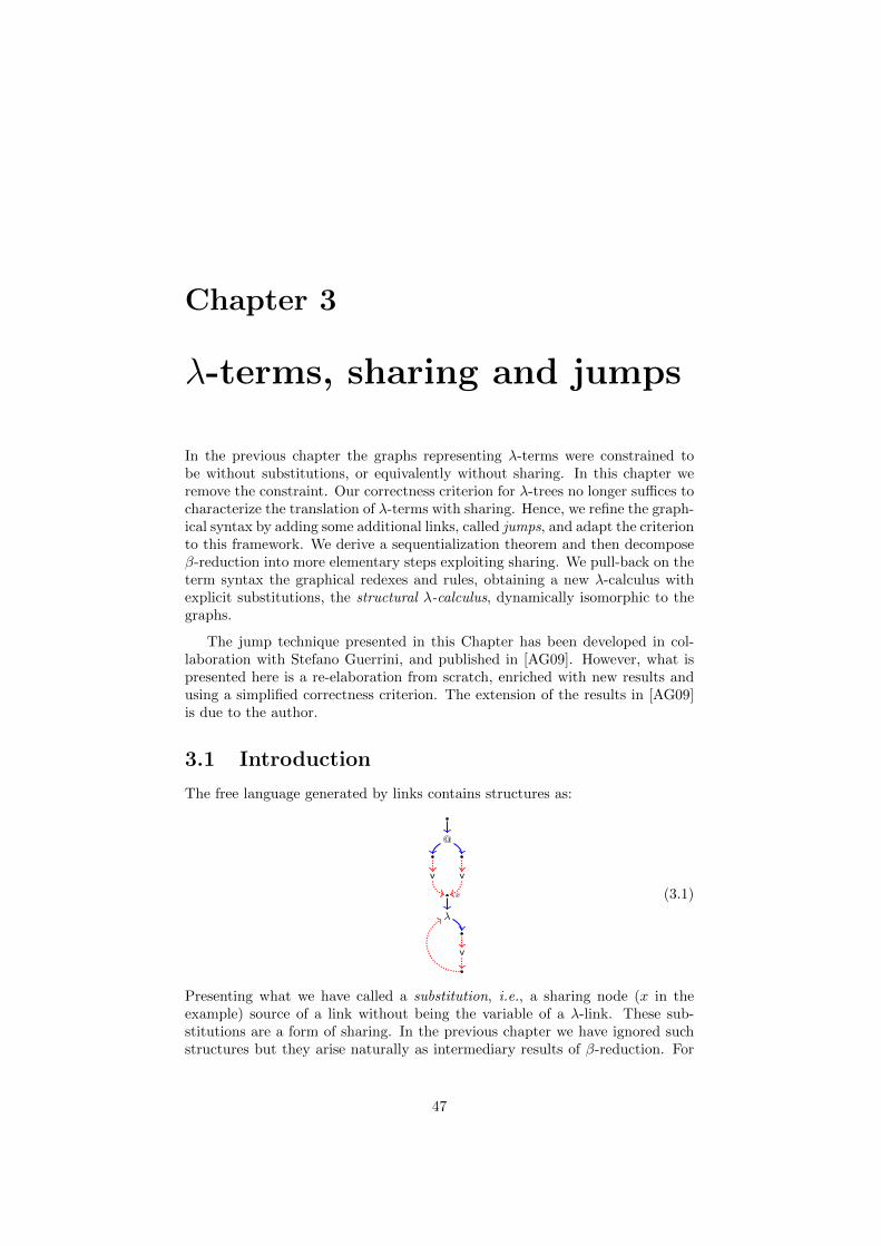
Chapter 3

λ-terms, sharing and jumps

In the previous chapter the graphs representing λ-terms were constrained tobe without substitutions, or equivalently without sharing. In this chapter weremove the constraint. Our correctness criterion for λ-trees no longer suffices tocharacterize the translation of λ-terms with sharing. Hence, we refine the graph-ical syntax by adding some additional links, called jumps, and adapt the criterionto this framework. We derive a sequentialization theorem and then decomposeβ-reduction into more elementary steps exploiting sharing. We pull-back on theterm syntax the graphical redexes and rules, obtaining a new λ-calculus withexplicit substitutions, the structural λ-calculus, dynamically isomorphic to thegraphs.

The jump technique presented in this Chapter has been developed in col-laboration with Stefano Guerrini, and published in [AG09]. However, what ispresented here is a re-elaboration from scratch, enriched with new results andusing a simplified correctness criterion. The extension of the results in [AG09]is due to the author.

3.1 Introduction

The free language generated by links contains structures as:

@

x

v v

v

λ

(3.1)

Presenting what we have called a substitution, i.e., a sharing node (x in theexample) source of a link without being the variable of a λ-link. These sub-stitutions are a form of sharing. In the previous chapter we have ignored suchstructures but they arise naturally as intermediary results of β-reduction. For

47

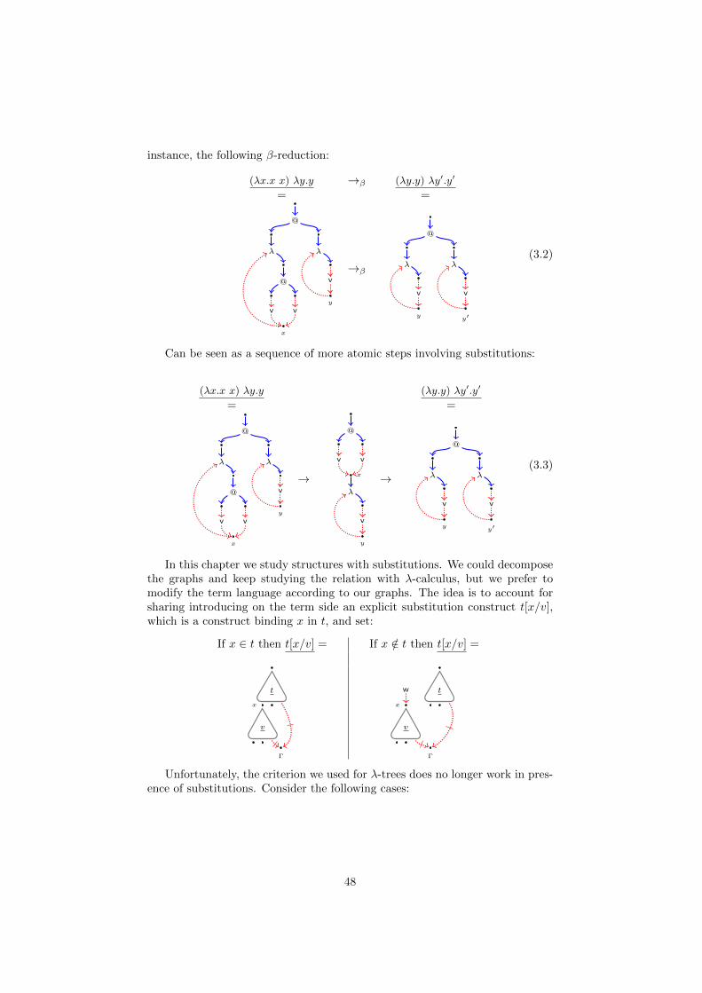
instance, the following β-reduction:

(λx.x x) λy.y →β (λy.y) λy′.y′

= =

@

@

x

v v

λ

y

v

λ

→β

@

y

v

λ

y′

v

λ(3.2)

Can be seen as a sequence of more atomic steps involving substitutions:

(λx.x x) λy.y (λy.y) λy′.y′

= =

@

@

x

v v

λ

y

v

λ

→

@

x

v v

y

v

λ

→

@

y

v

λ

y′

v

λ(3.3)

In this chapter we study structures with substitutions. We could decomposethe graphs and keep studying the relation with λ-calculus, but we prefer tomodify the term language according to our graphs. The idea is to account forsharing introducing on the term side an explicit substitution construct t[x/v],which is a construct binding x in t, and set:

If x ∈ t then t[x/v] = If x /∈ t then t[x/v] =

t

x

v

Γ

t

x

v

w

Γ

Unfortunately, the criterion we used for λ-trees does no longer work in pres-ence of substitutions. Consider the following cases:

48

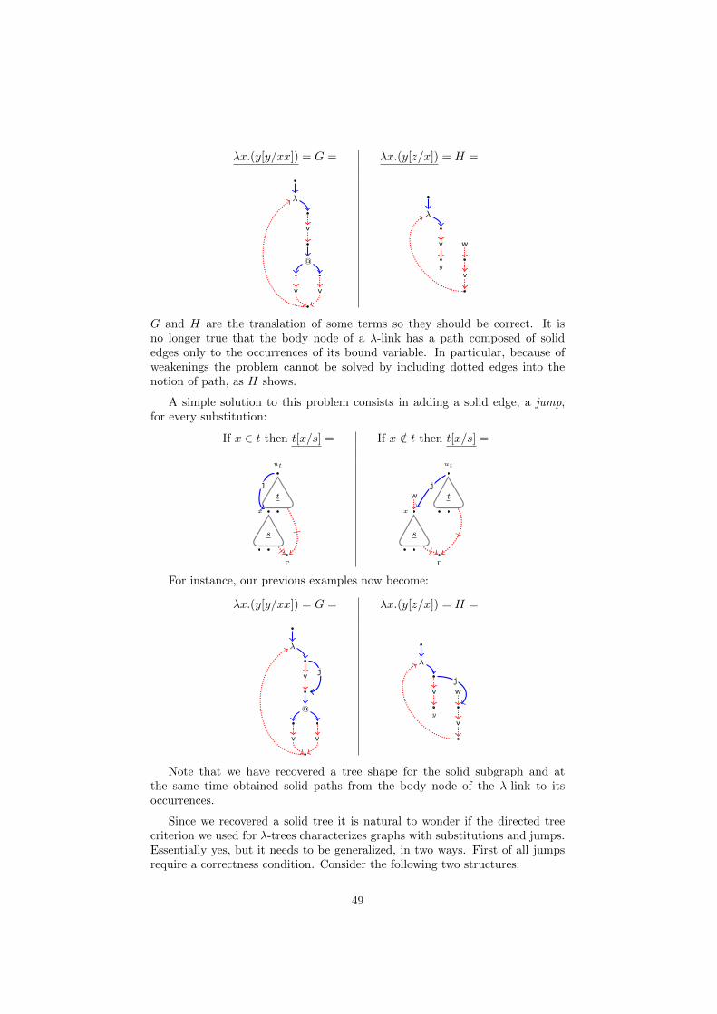
λx.(y[y/xx]) = G = λx.(y[z/x]) = H =

v

@

vv

λ

y

v w

v

λ

G and H are the translation of some terms so they should be correct. It isno longer true that the body node of a λ-link has a path composed of solidedges only to the occurrences of its bound variable. In particular, because ofweakenings the problem cannot be solved by including dotted edges into thenotion of path, as H shows.

A simple solution to this problem consists in adding a solid edge, a jump,for every substitution:

If x ∈ t then t[x/s] = If x /∈ t then t[x/s] =

ut

t

x

s

Γ

j

ut

t

x

s

w

Γ

j

For instance, our previous examples now become:

λx.(y[y/xx]) = G = λx.(y[z/x]) = H =

v

@

vv

λ

j

y

v w

v

λ

j

Note that we have recovered a tree shape for the solid subgraph and atthe same time obtained solid paths from the body node of the λ-link to itsoccurrences.

Since we recovered a solid tree it is natural to wonder if the directed treecriterion we used for λ-trees characterizes graphs with substitutions and jumps.Essentially yes, but it needs to be generalized, in two ways. First of all jumpsrequire a correctness condition. Consider the following two structures:

49

@

@

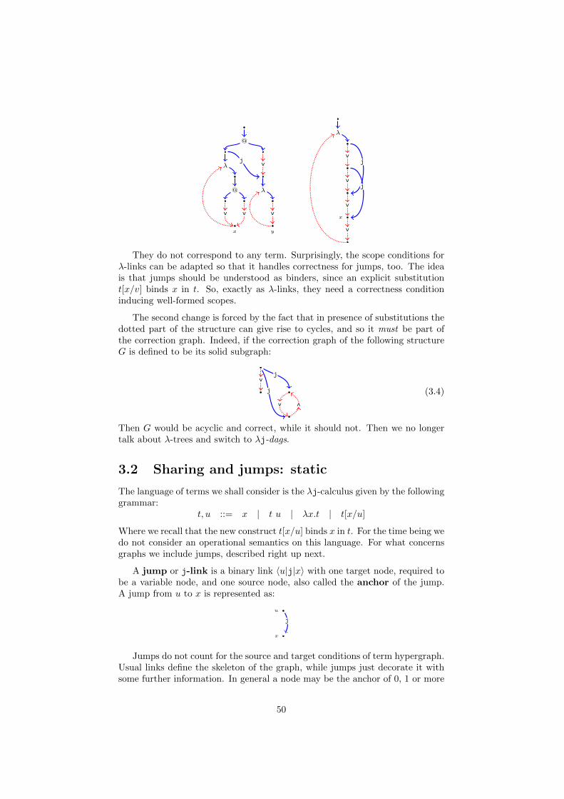
x

v v

λ v

y

v

λ

j

x

v

v

v

v

λ

j

j

They do not correspond to any term. Surprisingly, the scope conditions forλ-links can be adapted so that it handles correctness for jumps, too. The ideais that jumps should be understood as binders, since an explicit substitutiont[x/v] binds x in t. So, exactly as λ-links, they need a correctness conditioninducing well-formed scopes.

The second change is forced by the fact that in presence of substitutions thedotted part of the structure can give rise to cycles, and so it must be part ofthe correction graph. Indeed, if the correction graph of the following structureG is defined to be its solid subgraph:

v

vv

j

j (3.4)

Then G would be acyclic and correct, while it should not. Then we no longertalk about λ-trees and switch to λj-dags.

3.2 Sharing and jumps: static

The language of terms we shall consider is the λj-calculus given by the followinggrammar:

t, u ::= x | t u | λx.t | t[x/u]

Where we recall that the new construct t[x/u] binds x in t. For the time being wedo not consider an operational semantics on this language. For what concernsgraphs we include jumps, described right up next.

A jump or j-link is a binary link 〈u|j|x〉 with one target node, required tobe a variable node, and one source node, also called the anchor of the jump.A jump from u to x is represented as:

u

x

j

Jumps do not count for the source and target conditions of term hypergraph.Usual links define the skeleton of the graph, while jumps just decorate it withsome further information. In general a node may be the anchor of 0, 1 or more

50

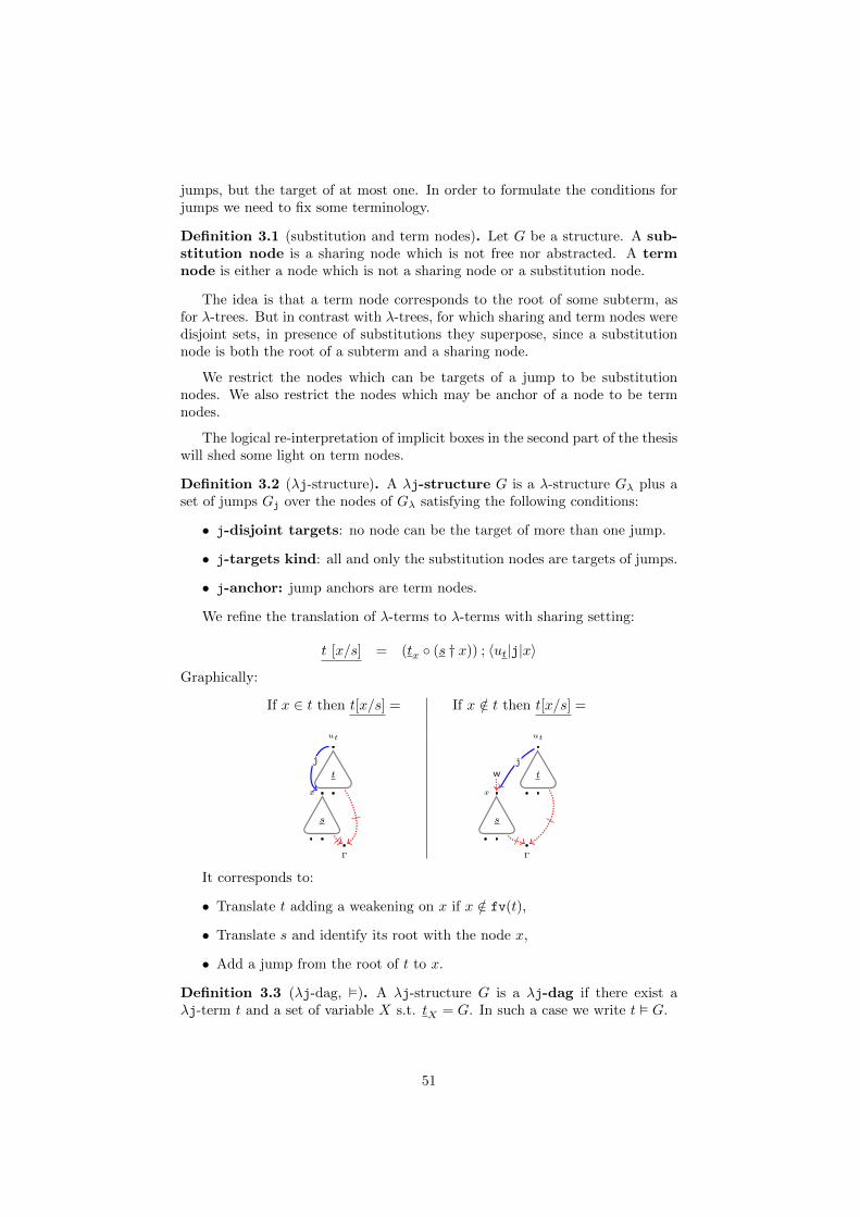
jumps, but the target of at most one. In order to formulate the conditions forjumps we need to fix some terminology.

Definition 3.1 (substitution and term nodes). Let G be a structure. A sub-stitution node is a sharing node which is not free nor abstracted. A termnode is either a node which is not a sharing node or a substitution node.

The idea is that a term node corresponds to the root of some subterm, asfor λ-trees. But in contrast with λ-trees, for which sharing and term nodes weredisjoint sets, in presence of substitutions they superpose, since a substitutionnode is both the root of a subterm and a sharing node.

We restrict the nodes which can be targets of a jump to be substitutionnodes. We also restrict the nodes which may be anchor of a node to be termnodes.

The logical re-interpretation of implicit boxes in the second part of the thesiswill shed some light on term nodes.

Definition 3.2 (λj-structure). A λj-structure G is a λ-structure Gλ plus aset of jumps Gj over the nodes of Gλ satisfying the following conditions:

• j-disjoint targets: no node can be the target of more than one jump.

• j-targets kind: all and only the substitution nodes are targets of jumps.

• j-anchor: jump anchors are term nodes.

We refine the translation of λ-terms to λ-terms with sharing setting:

t [x/s] = (tx (s † x)) ; 〈ut|j|x〉

Graphically:

If x ∈ t then t[x/s] = If x /∈ t then t[x/s] =

ut

t

x

s

Γ

j

ut

t

x

s

w

Γ

j

It corresponds to:

• Translate t adding a weakening on x if x /∈ fv(t),

• Translate s and identify its root with the node x,

• Add a jump from the root of t to x.

Definition 3.3 (λj-dag, ). A λj-structure G is a λj-dag if there exist aλj-term t and a set of variable X s.t. tX = G. In such a case we write t G.

51

'

&

$

%

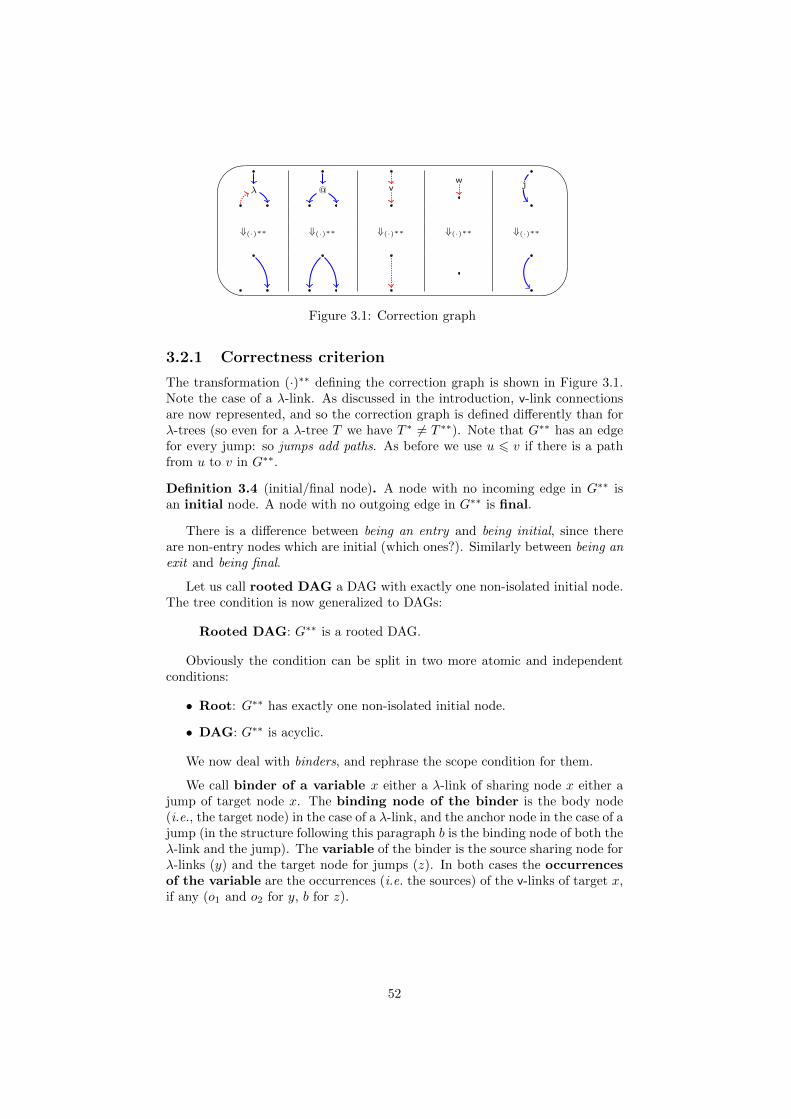
λ @ vw j

⇓(·)∗∗ ⇓(·)∗∗ ⇓(·)∗∗ ⇓(·)∗∗ ⇓(·)∗∗

Figure 3.1: Correction graph

3.2.1 Correctness criterion

The transformation (·)∗∗ defining the correction graph is shown in Figure 3.1.Note the case of a λ-link. As discussed in the introduction, v-link connectionsare now represented, and so the correction graph is defined differently than forλ-trees (so even for a λ-tree T we have T ∗ 6= T ∗∗). Note that G∗∗ has an edgefor every jump: so jumps add paths. As before we use u 6 v if there is a pathfrom u to v in G∗∗.

Definition 3.4 (initial/final node). A node with no incoming edge in G∗∗ isan initial node. A node with no outgoing edge in G∗∗ is final.

There is a difference between being an entry and being initial, since thereare non-entry nodes which are initial (which ones?). Similarly between being anexit and being final.

Let us call rooted DAG a DAG with exactly one non-isolated initial node.The tree condition is now generalized to DAGs:

Rooted DAG: G∗∗ is a rooted DAG.

Obviously the condition can be split in two more atomic and independentconditions:

• Root: G∗∗ has exactly one non-isolated initial node.

• DAG: G∗∗ is acyclic.

We now deal with binders, and rephrase the scope condition for them.

We call binder of a variable x either a λ-link of sharing node x either ajump of target node x. The binding node of the binder is the body node(i.e., the target node) in the case of a λ-link, and the anchor node in the case of ajump (in the structure following this paragraph b is the binding node of both theλ-link and the jump). The variable of the binder is the source sharing node forλ-links (y) and the target node for jumps (z). In both cases the occurrencesof the variable are the occurrences (i.e. the sources) of the v-links of target x,if any (o1 and o2 for y, b for z).

52

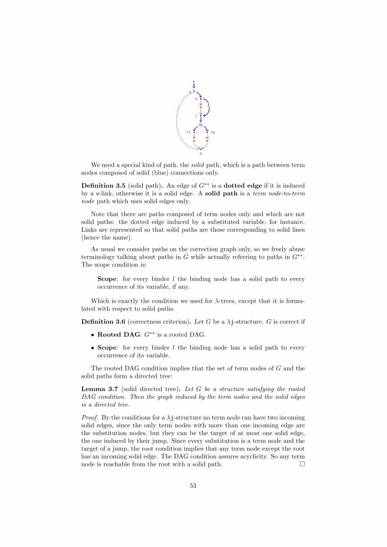
b

z

v

o1 o2

@

y

vv

λ

j

We need a special kind of path, the solid path, which is a path between termnodes composed of solid (blue) connections only.

Definition 3.5 (solid path). An edge of G∗∗ is a dotted edge if it is inducedby a v-link, otherwise it is a solid edge. A solid path is a term node-to-termnode path which uses solid edges only.

Note that there are paths composed of term nodes only and which are notsolid paths: the dotted edge induced by a substituted variable, for instance.Links are represented so that solid paths are those corresponding to solid lines(hence the name).

As usual we consider paths on the correction graph only, so we freely abuseterminology talking about paths in G while actually referring to paths in G∗∗.The scope condition is:

Scope: for every binder l the binding node has a solid path to everyoccurrence of its variable, if any.

Which is exactly the condition we used for λ-trees, except that it is formu-lated with respect to solid paths.

Definition 3.6 (correctness criterion). Let G be a λj-structure. G is correct if

• Rooted DAG: G∗∗ is a rooted DAG.

• Scope: for every binder l the binding node has a solid path to everyoccurrence of its variable.

The rooted DAG condition implies that the set of term nodes of G and thesolid paths form a directed tree:

Lemma 3.7 (solid directed tree). Let G be a structure satisfying the rootedDAG condition. Then the graph induced by the term nodes and the solid edgesis a directed tree.

Proof. By the conditions for a λj-structure no term node can have two incomingsolid edges, since the only term nodes with more than one incoming edge arethe substitution nodes, but they can be the target of at most one solid edge,the one induced by their jump. Since every substitution is a term node and thetarget of a jump, the root condition implies that any term node except the roothas an incoming solid edge. The DAG condition assures acyclicity. So any termnode is reachable from the root with a solid path.

53

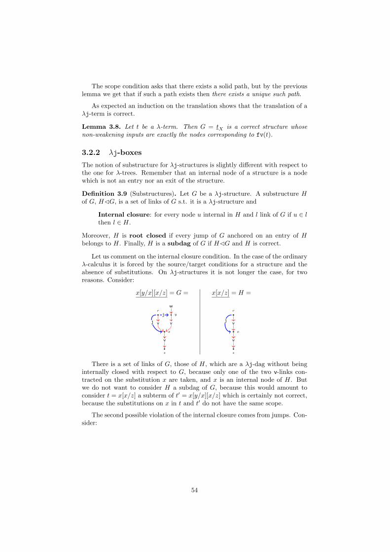
The scope condition asks that there exists a solid path, but by the previouslemma we get that if such a path exists then there exists a unique such path.

As expected an induction on the translation shows that the translation of aλj-term is correct.

Lemma 3.8. Let t be a λ-term. Then G = tX is a correct structure whosenon-weakening inputs are exactly the nodes corresponding to fv(t).

3.2.2 λj-boxes

The notion of substructure for λj-structures is slightly different with respect tothe one for λ-trees. Remember that an internal node of a structure is a nodewhich is not an entry nor an exit of the structure.

Definition 3.9 (Substructures). Let G be a λj-structure. A substructure Hof G, HCG, is a set of links of G s.t. it is a λj-structure and

Internal closure: for every node u internal in H and l link of G if u ∈ lthen l ∈ H.

Moreover, H is root closed if every jump of G anchored on an entry of Hbelongs to H. Finally, H is a subdag of G if HCG and H is correct.

Let us comment on the internal closure condition. In the case of the ordinaryλ-calculus it is forced by the source/target conditions for a structure and theabsence of substitutions. On λj-structures it is not longer the case, for tworeasons. Consider:

x[y/x][x/z] = G = x[x/z] = H =

ry

w

j

x

vv

z

v

j

r

x

v

z

v

j

There is a set of links of G, those of H, which are a λj-dag without beinginternally closed with respect to G, because only one of the two v-links con-tracted on the substitution x are taken, and x is an internal node of H. Butwe do not want to consider H a subdag of G, because this would amount toconsider t = x[x/z] a subterm of t′ = x[y/x][x/z] which is certainly not correct,because the substitutions on x in t and t′ do not have the same scope.

The second possible violation of the internal closure comes from jumps. Con-sider:

54

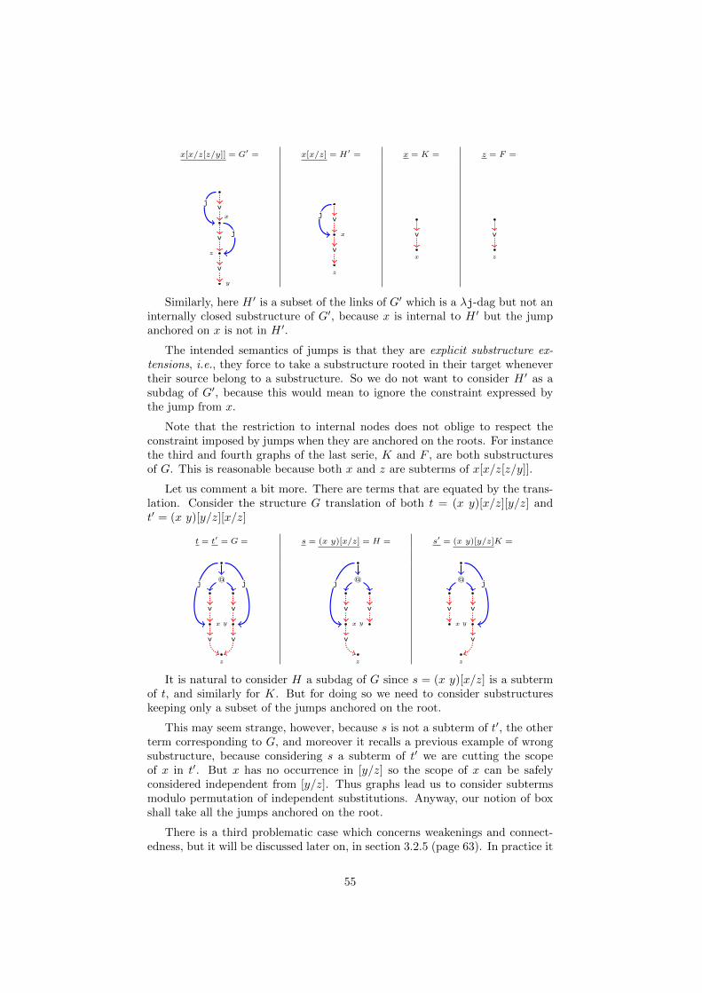
x[x/z[z/y]] = G′ = x[x/z] = H′ = x = K = z = F =

x

v

z

v

j

y

v

j x

v

z

v

j

x

v

z

v

Similarly, here H ′ is a subset of the links of G′ which is a λj-dag but not aninternally closed substructure of G′, because x is internal to H ′ but the jumpanchored on x is not in H ′.

The intended semantics of jumps is that they are explicit substructure ex-tensions, i.e., they force to take a substructure rooted in their target whenevertheir source belong to a substructure. So we do not want to consider H ′ as asubdag of G′, because this would mean to ignore the constraint expressed bythe jump from x.

Note that the restriction to internal nodes does not oblige to respect theconstraint imposed by jumps when they are anchored on the roots. For instancethe third and fourth graphs of the last serie, K and F , are both substructuresof G. This is reasonable because both x and z are subterms of x[x/z[z/y]].

Let us comment a bit more. There are terms that are equated by the trans-lation. Consider the structure G translation of both t = (x y)[x/z][y/z] andt′ = (x y)[y/z][x/z]

t = t′ = G = s = (x y)[x/z] = H = s′ = (x y)[y/z]K =

@

x

v

y

v

z

v v

j j @

x

v

y

v

z

v

j @

x

v

y

v

z

v

j

It is natural to consider H a subdag of G since s = (x y)[x/z] is a subtermof t, and similarly for K. But for doing so we need to consider substructureskeeping only a subset of the jumps anchored on the root.

This may seem strange, however, because s is not a subterm of t′, the otherterm corresponding to G, and moreover it recalls a previous example of wrongsubstructure, because considering s a subterm of t′ we are cutting the scopeof x in t′. But x has no occurrence in [y/z] so the scope of x can be safelyconsidered independent from [y/z]. Thus graphs lead us to consider subtermsmodulo permutation of independent substitutions. Anyway, our notion of boxshall take all the jumps anchored on the root.

There is a third problematic case which concerns weakenings and connect-edness, but it will be discussed later on, in section 3.2.5 (page 63). In practice it

55

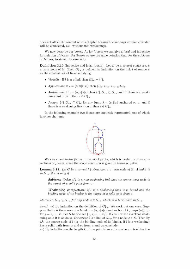
does not affect the content of this chapter because the subdags we shall considerwill be connected, i.e., without free weakenings.

We now describe our boxes. As for λ-trees we can give a local and inductiveformulation of jboxes. For jboxes we use the same notation than for the subtreesof λ-trees, to stress the similarity.

Definition 3.10 (inductive and local jboxes). Let G be a correct structure, ua term node of G. Then G↓u is defined by induction on the link l of source uas the smallest set of links satisfying:

• Variable: If l is a v-link then G↓u = l.

• Application: If l = 〈u|@|v, w〉 then l, G↓v, G↓w ⊆ G↓u.

• Abstraction: If l = 〈u, x|λ|v〉 then l, G↓v ⊆ G↓u and if there is a weak-ening link i on x then i ∈ G↓u.

• Jumps: j, G↓x ⊆ G↓u for any jump j = 〈u|j|x〉 anchored on u, and ifthere is a weakening link i on x then i ∈ G↓u.

In the following example two jboxes are explicitly represented, one of whichinvolves the jump:

v

@

vv

λ

j

We can characterize jboxes in terms of paths, which is useful to prove cor-rectness of jboxes, since the scope condition is given in terms of paths:

Lemma 3.11. Let G be a correct λj-structure, u a term node of G. A link l isin G↓u if and only if

Subterm links: if l is a non-weakening link then its source term node isthe target of a solid path from u.

Weakening completion: if l is a weakening then it is bound and thebinding node of its binder is the target of a solid path from u.

Moreover, G↓v ⊆ G↓u for any node v ∈ G↓u which is a term node in G↓u.

Proof. ⇒) By induction on the definition of G↓u. We work out one case. Sup-pose that u is the source of a λ-link i = 〈u, x|λ|v〉 and anchor of k jumps 〈u|j|xj〉for j = 1, . . . , k. Let S be the set v, x1, . . . , xk. If l is i or the eventual weak-ening on x it is obvious. Otherwise l is a link of G↓w for a node w ∈ S. Then byi.h. the source node of l (or the binding node of its binder, if l is a weakening)has a solid path from w and so from u and we conclude.⇐) By induction on the length k of the path from u to v, where v is either the

56

source term node of l or the binding node of its binder, if l is a weakening. Ifk = 0 it is obvious. Otherwise let u′ be the successor of u on the path from uto v. By i.h. l ∈ G↓u′ , which implies l ∈ G↓u.The moreover part is by induction on the definition of G↓u.

And now we prove that jboxes are correct.

Lemma 3.12 (jboxes are subdags). Let G be a correct λj-structure, u a termnode of G. Then G↓u is a connected and root closed subdag of G of root u, andu has a path to every exit of G↓u.

Proof. By induction on the definition of G↓u.Application: Suppose that u is the anchor of k jumps j1, . . . , jk of targetsx1, . . . , xk. Let us define S := v, w, x1, . . . , xk. The i.h. gives G↓z correctconnected substructure of G with root z, for every z ∈ S. In particular, everynode in S is internally closed in G↓u, because for x1, . . . , xk the scope conditionimplies that the occurrence of any v-link of target x1, . . . , xk has a solid pathfrom u, and thus by lemma 3.11 it is in G↓u. Note that if xi is the variable of aweakening then the weakening is taken. Since for every node in S G↓u containsits jbox we get that every x1, . . . , xk satisfies the j-targets kind condition. Allother internal nodes are internally closed by the i.h.. So G↓u is a substructure.Root condition: G↓u has only one non-isolated initial node, since u has a di-rected edge in G↓u to any node in S, and by i.h. the only non-isolated initialnode of G↓z is z, for z ∈ S.Scope condition: The only binders s.t. the scope condition does not follow fromthe i.h. are the jumps anchored on u. Consider xi for i = 1, . . . , k. We haveproved that it is an internal node of G↓u, so all the v-links of target xi are inG↓u, and by lemma 3.11 all their source nodes, i.e., all the occurrences of xi,have a solid path from u. So the scope condition holds.Acyclicity is obvious, and consequently G↓u is correct. Connectedness and thepath to the exits are evident by the i.h.. G↓u is root closed by definition.Variable: as the application case.Abstraction: Essentially as the application case. By the scope condition alloccurrences of x, if any, are in G↓v so G↓u is internally closed with respectto x and it respects the lambda condition (which is guaranteed by taking theweakening if x has no occurrence). The rest is as for the application case.

As before we get G = G↓r ;W for every correct λj-structure G of root r andfree weakenings W . For our notion of box we can prove the nesting property:

Lemma 3.13 (nesting). Let G be a correct structure and u, v two term nodesof G. Then G↓u ∩G↓v 6= ∅ implies G↓u ⊆ G↓v or G↓v ⊆ G↓u.

Proof. Suppose that I := G↓u ∩G↓v contains a non-weakening link l and let wbe its source term node. Then by correctness w has a solid path from v andu. Since there is only one maximal solid path ν to w (lemma 3.7), both u andv are on ν and so either u 6 v or v 6 u, and such paths are solid, which bylemma 3.11 implies the statement.If I contains a weakening l then by definition both jboxes contain its binder,whose binding node is a term node, and thus we reduce to the previous case.

57

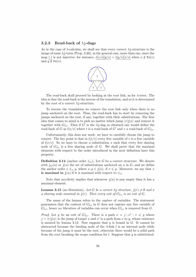
3.2.3 Read-back of λj-dags

As in the case of λ-calculus, we shall see that every correct λj-structure is theimage of some λj-term (Prop. 3.20), in the general case, more than one, since themap (·) is not injective; for instance, t[x/s][y/v] = t[y/v][x/s] when x /∈ fv(v)and y /∈ fv(s):

t

x

s

y

v

jj

The read-back shall proceed by looking at the root link, as for λ-trees. Theidea is that the read-back is the inverse of the translation, and so it is determinedby the root of a correct λj-structure.

To inverse the translation we remove the root link only when there is nojump anchored on the root. Thus, the read-back has to start by removing thejumps anchored on the root, if any, together with their substitutions. The firstidea that comes to mind is to pick no matter which jump 〈r|j|x〉 and remove ittogether with G↓x. Then if G′ is the λj-dag so obtained one would define theread-back of G as t[x/v] where t is a read-back of G′ and v a read-back of G↓x.

Unfortunately, this does not work: we have to carefully choose the jump toremove. The key point is that in t[x/v] every free variable of v is a free variableof t[x/v]. So we have to choose a substitution x such that every free sharingnode of G↓x is a free sharing node of G. We shall prove that the maximalelements with respect to the order introduced in the next definition have thisproperty.

Definition 3.14 (anchor order 6u). Let G be a correct structure. We denotewith jG(u) or j(u) the set of substitutions anchored on u in G, and we definethe anchor order x 6u y, where x, y ∈ j(u), if x 6 y. Moreover, we say that xis maximal in j(u) if it is maximal with respect to 6u.

Note that acyclicity implies that whenever j(u) is non empty then it has amaximal element.

Lemma 3.15 (no liberation). Let G be a correct λj-structure, j(r) 6= ∅ and xa sharing node maximal in j(r). Then every exit of G↓x is an exit of G.

The name of the lemma refers to the capture of variables. The statementguarantees that the context of G↓x in G does not capture any free variable ofG↓x, hence no liberation of variables can occur when G↓x is removed from G.

Proof. Let y be an exit of G↓x. There is a path ν = j ; ν′ : r 6 y wherej = 〈r|j|x〉 is the jump of target x and ν′ is a path from x to y, whose existenceis assured by lemma 3.12. Now suppose that y is bound in G. It cannot beabstracted because the binding node of the λ-link l is an internal node whilebecause of the jump it must be the root, otherwise there would be a solid pathfrom the root breaking the scope condition for l. Suppose that y is substituted.

58

Then its jump can only be anchored on the root. But by lemma 3.12 the root uof a jbox G↓u has a path to all the exits of G↓u, so that x 6 y, which contradictsmaximality of x. Hence y is an exit of G.

We introduce a notation for removals.

Definition 3.16 (removal G6↑x). If G is a correct λj-structure and x a substi-tution anchored on the root r of G then we use G6↑x for the structure G \ (G↓x ;〈x|j|r〉).

The next step is to prove that what is left after the removal of a maximalsubstitution is a correct structure, so that the read-back can continue induc-tively.

Lemma 3.17 (substitution splitting). Let G be a correct λj-structure of rootr, j(r) 6= ∅ and x a sharing node maximal in j(r). Then G6↑x is a correctλj-structure and G = (G6↑x G↓x) ; 〈x|j|r〉.

Proof. Lemma 3.15 implies G = (G6↑x G↓x) ; 〈x|j|r〉, that is, the equality holdsusing the free gluing and so no variable of G↓x is captured. The same lemmaand internal closure of G↓u imply that G6↑x is a subnet of G. Note that G↓uand G6↑x can only share u and the exits of G↓u, which are all exits of G6↑x bythe previous lemma and root closure of G↓u. Suppose that G6↑x has an initialnode v 6= r which is not an initial node of G. By internal closure of G↓u thiscan only happen if v is an interface node of G↓u and so v is an exit of G6↑x. Sov is both initial and final, i.e., it is isolated, and G 6↑x verifies the rooted DAGcondition.Let l be a binder of G 6↑x of binding node v and variable x. The condition forbeing a structure forces the variable of l to be an internal node of G6↑x. Thenby internal closure each occurrence o of x is in G6↑x, and so it has a solid pathτ from the root. Since by correctness of G v is on a solid path from the root too and the solid subgraph is a tree we get that v is a node of τ .

Now we have all the ingredients to define the read-back of a correct structureG in the case of jumps anchored on the root: a maximal substitution x alwaysexists, the free variables of G↓x are free variables of the structure, and thecontext G6↑x of G↓x in G is a correct structure, and so it can act as a subterm.

Whenever a correct structure G has some jumps anchored on the root weselect x maximal in j(r) and define the read-back as G = G6↑x[x/G↓x]. Butthe choice of x is not unique, and so the read-back is not a function, rather arelation. Hence we write G RB t:

Definition 3.18 (Read-back). Let G be a named correct structure of root r.A term t is a read-back of G, noted G RB t, if:

• If j(r) 6= ∅ then G RB s[x/v] where x is maximal in j(r), G6↑x RB s andG↓x RB v.

• Otherwise the read-back proceeds as before, namely:

〈r|v|x〉 ;G′ RB x〈r, x|λ|u〉 ;G′ RB λx.s if G↓u RB s〈r|@|u, v〉 ;G′ RB s1 s2 if G↓u RB s1 and G↓v RB s2

59

The well-definedness of the read-back is assured by the correctness of jboxes,by the substitution splitting lemma (which assures that G6↑x is correct) and bythe fact that j(r) has a maximal element whenever it is non-empty (by theacyclicity correctness condition).

For every node u of G which is anchor of some jumps every read back tof G induces a linearization of the substitutions in j(u), i.e., a total order 4uextending 6u. We then compactly say that 4, denoting the union of 4u for u

node of G, is a linearization of G, and write t = G4

. Sometimes we need toconsider the read-back of a substructure H of G with respect to the restriction

of 4 to H. In these cases we abuse notation and simply use H4

.

As in the previous chapter we need an @-splitting lemma, which is an im-mediate consequence of the nesting lemma.

Lemma 3.19 (@-splitting). Let G be a correct structure s.t. j(r) = ∅ and whoseoutput link is an @-link l = 〈r|@|u, v〉. Then G↓r = 〈r|@|u, v〉; (G↓u G↓v).

Proof. Since the link of source u is not in G↓v and the link of source v is notin G↓u we get G↓u 6⊆ G↓v and G↓v 6⊆ G↓u and by the nesting lemma the twojboxes cannot share any link. Suppose that they share a node u which is not anexit node. Then they share the only link of source u, which is absurd. So thetwo jboxes are freely glued.

Putting it all together we get:

Proposition 3.20 (the translation is the inverse of the read-back). Let G be

a correct structure without substitutions. Then G4 G for any linearization 4

of G, i.e., there exists a set of variables X s.t. (G4

)X

= G. Moreover, if G is

connected then X = ∅.

Proof. By induction on the number k of links. The proof is as for λ-trees exceptif k > 1, j(r) 6= ∅, and there are no isolated weakenings. In such a case, for asubstitution x maximal in j(r), we get:

(G4

) = G 6↑x4

[x/G↓u4

] =

((G6↑x4

) 〈w|x〉) (G↓x4

); 〈x|j|r〉 =i.h.

(G6↑x 〈w|x〉) G↓x; 〈x|j|r〉 =(1)

G6↑x G↓x; 〈x|j|r〉 =L.3.17 G

Where (1) is justified by the fact that G has a substitution on x and so G6↑xnecessarily has a link of source x.

Corollary 3.21 (Sequentialization). Let G be a λj-structure. G is a λj-dag iffit is correct.

Proof. ⇒) by induction on the definition of the translation. ⇐) Proposition3.20.

60

Lemma 3.22 (the read-back is complete). The read-back procedure is complete,that is, if t G then G RB t.

Proof. By induction on t. In the case s[x/v] we get that the pairs G6↑x and s,and G↓x and v, verifies the i.h. so that we get G6↑x RB s and G↓x RB v. Bydefinition of translation x is maximal in jG(r) and so we conclude by definitionof read-back.

We conclude this section by showing that the unique box theorem scales upto λj-dags.

Theorem 3.23 (unique box). Let G be a λj-dag, u term node of G. G↓u isthe unique connected and root closed subdag of G of root u.

Proof. Let H be a connected substructure of G of root u. If l is a non-weakeninglink of H then its source term node has a solid path from u in G and so by lemma3.11 l ∈ G↓u. If l is a weakening of H then it is bound by a binder i, becauseH is connected. Since i ∈ G↓u by definition of jbox l ∈ G↓u. Hence, H ⊆ G↓u.We prove by induction on the definition of G↓u that G↓u is contained in anyconnected and root closed subdag of G of root u. If j(u) = ∅ and u is thesource of a v-link l = 〈u|v|x〉 then G↓u = l and we conclude. Otherwise supposethat u is the source of k jumps j1, . . . , jk of targets x1, . . . , xk. Let us defineS := x, x1, . . . , xk. The i.h. gives G↓z contained in any connected and rootclosed subdag of G of root z, for every z ∈ S. Since H is root closed then Hcontains G↓u. The other cases are similar it is enough to put in S the targetnodes of the link l and then apply the same argument.

3.2.4 Domination criterion

In presence of the rooted DAG condition the scope condition can be reformulatedin terms of domination (domination is defined at page 41). In the rest of thissubsection we prove this fact.

Definition 3.24 (domination correctness). A λj-structure G is domination-correct if it satisfies the rooted DAG condition and the following:

Domination scope: If l is a binder of non-weakening variable x then thebinding node of l dominates x.

The following proposition is the key step to prove that the solid subtree ofG∗∗ coincide with its dominating tree order on term nodes.

Proposition 3.25 (domination and solid paths). Let G a structure. Then:

1. If G is dominating-correct then u v v implies that there is a solid pathfrom u to v, for any pair u, v of term nodes of G.

2. If G is correct and τ : u 6 v is a solid path then u v v, for any pair u, vof term nodes of G.

Proof. 1) Consider a path ν from the root to v. It factors as ν = ν0 ; ν1 whereν1 : u 6 v. We prove by induction on the number k of dotted edges of ν1 thatthere is a solid path from u to v. If k = 0 then ν1 is a solid path from u to v. If

61

k > 0 then consider the first dotted edge e = (o, x) of ν1. x is a substitution: if νcontinues after x this is obvious and if it does not then x = v and by hypothesisv is a term node, and the only nodes which are term and sharing nodes at thesame time are substitution nodes. Hence there is a jump j of target x. Theanchor w of j should be on ν1 otherwise the path going as ν0 until w, takingj and then continuing from x as ν1 is a path r 6 v from an initial node whichdoes not pass through u, against u v v, absurd. So w is on ν1 and replacingthe subpath τ : w 6 x of ν1 with j we get a path ν′1 which uses one dotted edgeless than ν1. We conclude by the i.h..2) Consider a path ν : r 6 v. We prove by induction on the number k of dottededges of ν that it passes through u. If k = 0 then ν is a solid path, but thereis only one maximal solid path to v, which is ν, so τ is a suffix of ν and νpasses through u. If k > 0 then consider the first dotted edge e = (o, x) on ν.The prefix ν0 : r 6 o of ν is then a solid path to o. As in the previous pointx is substituted: if ν continues after x this is obvious and if it does not thenx = v and by hypothesis v is a term node, and the only nodes which are termand sharing nodes at the same time are substitution nodes. So there is a jumpj = 〈w|j|x〉. By the scope condition there is a solid path σ : w 6 o, which is asuffix of ν0 by lemma 3.7. Then consider the path ν′ : r 6 v obtained from ν byreplacing σ ; e, which is a path from w to x, with j. ν′ uses strictly less dottededges of ν and by i.h. it passes through u. Every node of ν′ is a node of ν, sowe conclude.

Corollary 3.26 (domination tree=solid tree). Let G be a structure.

1. G is dominating-correct if and only if it is correct.

2. If G is correct then u v v if and only if there is a solid path u 6 v, forany two term nodes u and v of G.

Proof. We prove the first point, the second being an immediate consequence ofthe previous proposition. Let l be a binder of non-weakening variable x andbinding node v.⇒) v dominates all the occurrences of x so by the previous lemma it has a solidpath to each of them.⇐) v has a solid path to every occurrence of x so by the previous lemma itdominates all its occurrences and so it dominates x.

We can then obtain another characterization of jboxes:

Lemma 3.27. Let G be a correct λj-structure, u a term node of G. G↓u isthe set of links and jumps whose source term node is dominated by u, plus thebound weakenings whose binder is in G↓u.

Proof. By corollary 3.26.2 the definition of G↓u and the statement are equiva-lent.

For this reason G↓u is also called the dominion of u in G. Actually, this wasthe first characterization we found and the one used in the published versionof λj-dags [AG09]. The formulation in terms of solid paths from u originatedfrom the study of the generalization we shall present in the second part of thethesis, and the need to uniform their presentation.

62

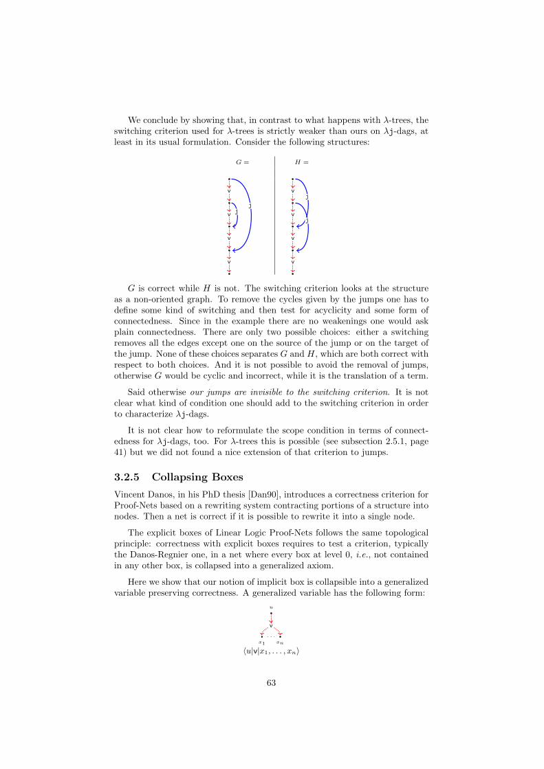
We conclude by showing that, in contrast to what happens with λ-trees, theswitching criterion used for λ-trees is strictly weaker than ours on λj-dags, atleast in its usual formulation. Consider the following structures:

G = H =

v

v

v

v

jj

v

v

v

v

j

j

G is correct while H is not. The switching criterion looks at the structureas a non-oriented graph. To remove the cycles given by the jumps one has todefine some kind of switching and then test for acyclicity and some form ofconnectedness. Since in the example there are no weakenings one would askplain connectedness. There are only two possible choices: either a switchingremoves all the edges except one on the source of the jump or on the target ofthe jump. None of these choices separates G and H, which are both correct withrespect to both choices. And it is not possible to avoid the removal of jumps,otherwise G would be cyclic and incorrect, while it is the translation of a term.

Said otherwise our jumps are invisible to the switching criterion. It is notclear what kind of condition one should add to the switching criterion in orderto characterize λj-dags.

It is not clear how to reformulate the scope condition in terms of connect-edness for λj-dags, too. For λ-trees this is possible (see subsection 2.5.1, page41) but we did not found a nice extension of that criterion to jumps.

3.2.5 Collapsing Boxes

Vincent Danos, in his PhD thesis [Dan90], introduces a correctness criterion forProof-Nets based on a rewriting system contracting portions of a structure intonodes. Then a net is correct if it is possible to rewrite it into a single node.

The explicit boxes of Linear Logic Proof-Nets follows the same topologicalprinciple: correctness with explicit boxes requires to test a criterion, typicallythe Danos-Regnier one, in a net where every box at level 0, i.e., not containedin any other box, is collapsed into a generalized axiom.

Here we show that our notion of implicit box is collapsible into a generalizedvariable preserving correctness. A generalized variable has the following form:

u

x1 xn

v

. . .

〈u|v|x1, . . . , xn〉

63

And it is the λ-calculus analogous of a generalized axiom. Its source is a termnode and its targets are sharing nodes. Correctness is extended by consideringthe source node of a generalized variable an occurrence of its targets, if they arebound. Sequentialization extends smoothly.

We characterize all the subdags for which the collapsing preserves correct-ness.

Definition 3.28 (collapse). Let G be a λj-dag, HCG a subdag of exits ∆ =x1, . . . , xk and root rH , G = G′ ∝ H. We define the collapse G÷H of H inG as G where H has been replaced with a generalized variable having the sameinterface, formally G÷H := G′ ∝ 〈rH |v|∆〉.

Proposition 3.29. Let G be a λj-dag, HCG a subdag. G÷H is correct ⇔ forevery free weakening l = 〈w|x〉 of H

1. x has no path to rH in G.

2. If x is bound by a binder l in G then the binding node u of l has a solidpath to rH .

Proof. ⇒) Suppose that there is a free weakening l = 〈w|x〉 of H bound by abinder l whose binding node u has no solid path to rH . Then rH becomes anoccurrence of x in G÷H and the scope condition for l does not hold. If x hasa path to rH in G it is immediate that G÷H has a cycle, absurd.⇐) The only edges of G÷H for which there is no coinitial and cofinal path inG are the edges from the root rH of H and the eventual nodes x1, . . . , xk ofthe free weakenings of H.Root : none among x1, . . . , xk can be the root of G, so the root condition ispreserved.Acyclicity : if there is a cycle then there exists i s.t. xi has a path to rH inG÷H, and thus in G. But this contradicts the hypothesis, absurd.Scope: Let l a binder of G of binding node u and variable x. If it has anoccurrence o in H then u has a solid path to rH . In G÷H the node rH takesthe place of o as occurrence of x, and so we conclude. If x ∈ x1, . . . , xk then xgets as occurrence rH but by hypothesis there is a solid path from u to rH . If xhas an occurrence not in H then the solid path τ from u cannot use any edge ofH, because by internal closure it has to use an edge from rH to an internal nodeof H, and then any other solid edge from internal nodes of H is in H so that owould be an occurrence of H. Then τ is a path of G÷H and we conclude.

We instantiate the proposition on jboxes:

Corollary 3.30. Let G be a λj-dag and u a term node of G. Then G÷G↓u iscorrect.

Proof. It immediately follows from proposition 3.29, since jboxes have no freeweakening.

3.3 Graphical quotient

The characterization of the graphical quotient induced by the translation re-quires to restrict to well-named terms: we recall that a term t is well-named

64

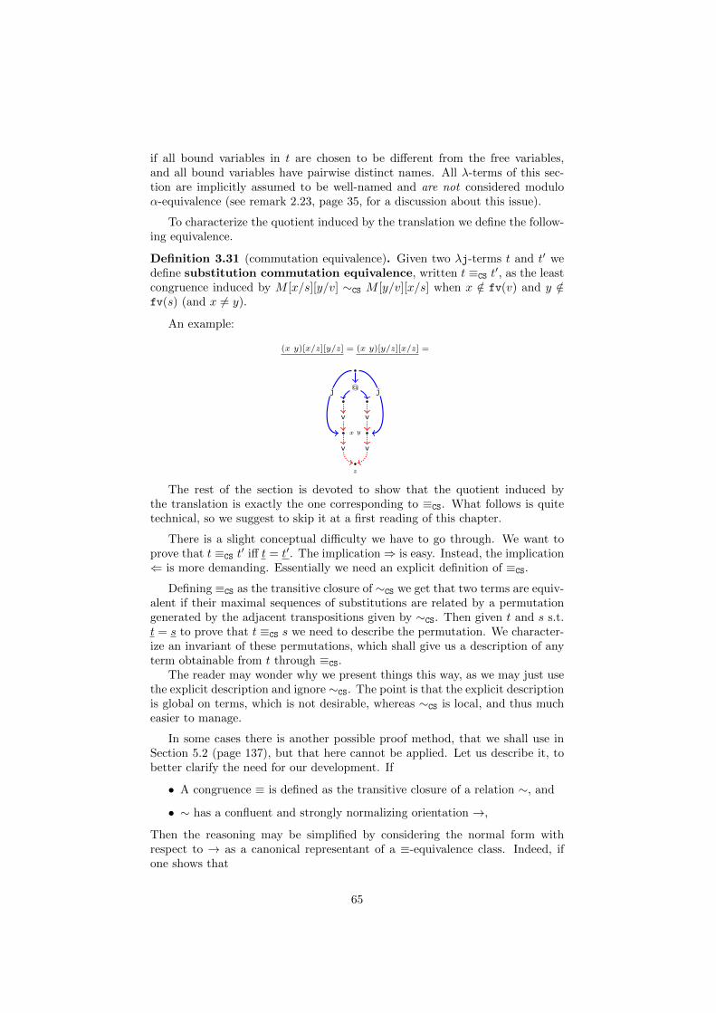
if all bound variables in t are chosen to be different from the free variables,and all bound variables have pairwise distinct names. All λ-terms of this sec-tion are implicitly assumed to be well-named and are not considered moduloα-equivalence (see remark 2.23, page 35, for a discussion about this issue).

To characterize the quotient induced by the translation we define the follow-ing equivalence.

Definition 3.31 (commutation equivalence). Given two λj-terms t and t′ wedefine substitution commutation equivalence, written t ≡CS t

′, as the leastcongruence induced by M [x/s][y/v] ∼CS M [y/v][x/s] when x /∈ fv(v) and y /∈fv(s) (and x 6= y).

An example:

(x y)[x/z][y/z] = (x y)[y/z][x/z] =

@

x

v

y

v

z

v v

j j

The rest of the section is devoted to show that the quotient induced bythe translation is exactly the one corresponding to ≡CS. What follows is quitetechnical, so we suggest to skip it at a first reading of this chapter.

There is a slight conceptual difficulty we have to go through. We want toprove that t ≡CS t

′ iff t = t′. The implication⇒ is easy. Instead, the implication⇐ is more demanding. Essentially we need an explicit definition of ≡CS.

Defining ≡CS as the transitive closure of ∼CS we get that two terms are equiv-alent if their maximal sequences of substitutions are related by a permutationgenerated by the adjacent transpositions given by ∼CS. Then given t and s s.t.t = s to prove that t ≡CS s we need to describe the permutation. We character-ize an invariant of these permutations, which shall give us a description of anyterm obtainable from t through ≡CS.

The reader may wonder why we present things this way, as we may just usethe explicit description and ignore ∼CS. The point is that the explicit descriptionis global on terms, which is not desirable, whereas ∼CS is local, and thus mucheasier to manage.

In some cases there is another possible proof method, that we shall use inSection 5.2 (page 137), but that here cannot be applied. Let us describe it, tobetter clarify the need for our development. If

• A congruence ≡ is defined as the transitive closure of a relation ∼, and

• ∼ has a confluent and strongly normalizing orientation →,

Then the reasoning may be simplified by considering the normal form withrespect to → as a canonical representant of a ≡-equivalence class. Indeed, ifone shows that

65

• ∼-equivalent terms are mapped on the same graph,

• The translation from terms to graphs is injective with respect to→-normalforms.

Then ≡ is the quotient induced by the translation. Unfortunately, ∼CS does notadmit a strongly normalizing orientation, because it is a commutative relation,and so we have to reformulate it globally. However, we suspect that what shallfollow is a bit over-complicated, but we leave its eventual simplification to futurework.

There are two things we have to reformulate, one is the context closure,which shall be substituted with a definition by induction, the other is the clo-sure by transitivity, which shall require an order over the maximal sequencesof substitutions. This order is essentially the transitive closure of the ordercontaining an occurrence of :

Definition 3.32. Let t = v[x1/s1] . . . [xk/sk] with v a term which is not anexplicit substitution. We define xi ≺1

t xj in t if xj ∈ si and 1 ≤ i, j ≤ k, andxi ≺t xj as the transitive closure of ≺1

t .

In the previous definition the case where xi = xj for some indexes i, j isruled out by the fact that we consider well-named terms only.

Definition 3.33. We define t l t′ by induction on t.

• If t = x then t l t′ if t′ = x

• If t = λx.s then t l t′ if t′ = λx.s′ and s l s′.

• If t = s v then t l t′ if t′ = s′ v′, s l s′ and v l v′.

• Let t = v[x1/s1] . . . [xk/sk], k > 0 and v not an explicit substitution thent l t′ if

– t′ = v′[xi1/s′i1

] . . . [xik/s′ik

] where K = 1, . . . , k = i1, . . . , ik,– v l v′, si l s′i for i ∈ K,

– v′ is not an explicit substitution, and

– The partial orders (X,≺t) and (X,≺t′), where X = x1, . . . , xk,coincide.

Lemma 3.34. t ≡CS t′ iff t l t′.

Proof. ⇒) It is enough to note that ∼CS preserves the partial orders in thedefinition of t l t′. ⇐) By induction on t. The only interesting case is when t =v[x1/s1] . . . [xk/sk]. We use the notation of the definition of l plus ≺:=≺t=≺t′ .t and t′ corresponds to two different total orders on X = x1, . . . , xk containing≺. By the i.h.we get that si ≡CS s

′i for i ∈ K and v ≡CS v

′. Let τ be thepermutation on K s.t. τ(j) = l if j = il, for j, l ∈ K. Note that, since bothtotal orders contains ≺, x < y are inverted by τ , i.e., τ(y) < τ(x), only if x 6≺ yand y 6≺ x. We prove t ≡CS t

′ by induction on the number n of inversions of τ .If n = 0 then just use the i.h. on the subterms of t. If n > 0 then consider theterm:

t′′ = v[xi1/si1 ] . . . [xik/sik ]

66

Which is t′ where the subterms v′, s′1, . . . , s′k have been replaced by their ≡CS-

equivalent ones in t. Clearly t′ ≡CS t′′ and t l t′′. Now let j be the minimal

element of K inverted by τ , i.e., s.t. ij 6= j. Consider the position l = τ(j) ofxj in t′′. Minimality of j implies that xil and xil−1

form an inversion for τ , andso they are ≺-unrelated. In particular xil /∈ sil−1

and xil−1/∈ sil . So consider

t′′′ = v[xi1/si1 ] . . . [xil−2/sil−2

][xil/sil ][xil−1/sil−1

][xil+1/sil+1

] . . . [xik/sik ]

Which is t′′ where the substitutions of xil and xil−1have been swapped. We

get t′′ ∼CS t′′′ and so t′′ ≡CS t

′′′. Consider the permutation τ ′ relating t and t′′′.τ ′ is equal to τ everywhere except on τ−1(l) = j and τ−1(l − 1), whose valueare swapped. By minimality of j the permutation τ ′ has an inversion less thanτ and so t ≡CS t

′′′ by i.h.. Thus t ≡CS t′′′ ≡CS t

′′ ≡CS t′.

We still have to relate the order ≺t and the λj-dag of t. It turns out that ≺tcoincides with the partial order 6r on the substitutions anchored on the root,which was introduced to define the read-back. We need a preliminary lemma,which is a sort of converse of the no liberation lemma.

Lemma 3.35. Let G be a λj-dag with |j(r)| = k > 0 and x, y ∈ j(r). There isa path τ : x 6 y and there is no element of j(r) \ x, y in τ if and only if y isa free sharing node of jbox(x).

Proof. ⇒) Let us prove that y ∈ G↓x. Suppose by contradiction that y /∈ G↓x.Then let v be the last term node of G↓x on ρ : x 6 y. If v = y then by lemma3.11 G↓y ⊆ G↓x and in particular y ∈ G↓x. So v 6= y and by maximality of itsposition on ρ the node right after it on ρ is a sharing node z of G↓x. If z issubstituted in G↓x then v is not the last term node of G↓x on ρ, absurd. If zis abstracted in G↓x then it has no outgoing edge, so z = y and y abstracted,absurd. So z is free in G↓x. Now if z 6= y then ρ continues after z and z is thetarget of a jump j, which is necessarily anchored on the root, and so there is anode of j(r) \ x, y in τ , absurd. So z = y, and we conclude.⇐) In a jbox the root has a path to every free sharing node (lemma 3.12), andso there exists a path τ : x 6 y. The link of any substitution node z on ρ is inG↓x so by lemma 3.11 it has a solid path from x and thus it cannot be anchoredon the root.

Lemma 3.36 (6r=≺t). Let G be a λj-dag with |j(r)| = k > 0. If tX = G thent = v[x1/s1] . . . [xk/sk], and xi 6r xj iff xi ≺t xj.

Proof. The only term constructor whose translation puts a jump on the rootis the explicit substitution, and any other construct changes the root link, sot = v[x1/s1] . . . [xk/sk], with si G↓xi for i ∈ K = 1, . . . , k.⇒) Suppose that xi 6r xj and consider a path ρ : xi 6 xj . We prove xi ≺t xjby induction on the number d of elements of j(r) \ xi, xj in ρ.If d = 0 then by lemma 3.35 xj is a free sharing node of G↓xi , i.e., xj ∈ fv(si),and so xi ≺t xj . If d > 1 let xl an element of j(r) \ xi, xj on ρ. We split ρ onxl, getting two subpaths, apply the i.h. twice obtaining xi ≺t xl and xl ≺t xj ,and conclude xi ≺t xj by transitivity.⇐) If xi ≺t xj because xj ∈ si then by lemma 3.8 xj is a non-weakening exit ofsi, and by correctness there is a path from the root rsi of si to xj . By hypothesisrsi is xi, and so xi 6r xj .The inductive case of xi ≺t xj is a straightforward use of the i.h..

67

Now we can conclude:

Theorem 3.37 (graphical quotient). Let t, u be λj-terms and G a named λj-dag. t G and u G iff t ≡CS t

′.

Proof. ⇐) Just observe that t ∼CS u implies t = u as a named λj-dag. Theproperty clearly is preserved by the transitive and contextual closure of ∼CS.⇒) The proof is by induction on the number of links of G, by looking at theroot. If j(r) = ∅ or if there is any free weakening then just use the i.h., as inthe proof of lemma 2.22 (page 35). The interesting case is if |j(r)| = k > 0. Bylemma 3.36 t has the form t = v[x1/s1] . . . [xk/sk], where

• si = G↓xi

• There exists X s.t. vX = G6↑xk . . . 6↑x1

• v is not an explicit substitution

• xi 6r xj iff xi ≺t xj , that is, (X,6r) and (X,≺t) coincide, where X =x1, . . . , xk.

Similarly t′ has the form t′ = v′[xi1/s′i1

] . . . [xik/s′ik

] where K = 1, . . . , k =i1, . . . , ik, and

• s′i = G↓xi

• There exists Y s.t. vY = G6↑xik . . . 6↑xi1• v′ is not an explicit substitution

• (X,6r) and (X,≺t′) coincide.

We get si = s′i and so by the i.h. si ≡CS s′i, for i ∈ K. Then vX = v′Y and

by the i.h. v ≡CS v′. By lemma 3.34 v l v′ and si l s′i. So t l t′, that is,

t ≡CS t′.

Since the read-back is the inverse of the translation the result can obviouslybe rephrased using the read-back:

Corollary 3.38. Let t and u be two read-backs of a named λj-dag G. Thent ≡CS u.

3.4 Dynamics

We endow λj-dags with an operational semantics inspired by Linear Logic Proof-Nets. No previous knowledge of Linear Logic is required. However, the inter-ested reader will find the connection between the two formalisms in Chapter5.

68

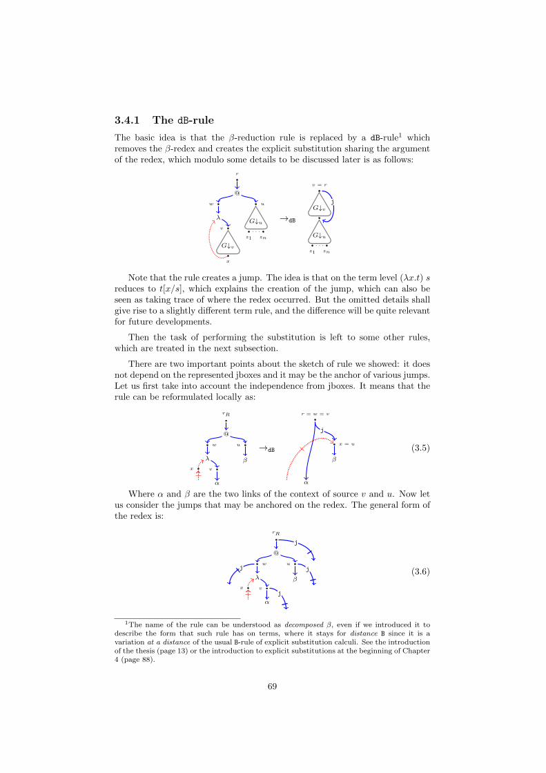
3.4.1 The dB-rule

The basic idea is that the β-reduction rule is replaced by a dB-rule1 whichremoves the β-redex and creates the explicit substitution sharing the argumentof the redex, which modulo some details to be discussed later is as follows:

r

w u

@

G↓u

z1 zn

. . .v

G↓v

x

λ →dB

v = r

G↓v

x

G↓u

z1 zn

. . .

j

Note that the rule creates a jump. The idea is that on the term level (λx.t) sreduces to t[x/s], which explains the creation of the jump, which can also beseen as taking trace of where the redex occurred. But the omitted details shallgive rise to a slightly different term rule, and the difference will be quite relevantfor future developments.

Then the task of performing the substitution is left to some other rules,which are treated in the next subsection.

There are two important points about the sketch of rule we showed: it doesnot depend on the represented jboxes and it may be the anchor of various jumps.Let us first take into account the independence from jboxes. It means that therule can be reformulated locally as:

rR

w u

@

β

v

α

x

λ

→dB

r = w = v

x = u

β

α

j

(3.5)

Where α and β are the two links of the context of source v and u. Now letus consider the jumps that may be anchored on the redex. The general form ofthe redex is:

rR

j

w u

@

β

j

v

α

jx

λ

j(3.6)

1The name of the rule can be understood as decomposed β, even if we introduced it todescribe the form that such rule has on terms, where it stays for distance B since it is avariation at a distance of the usual B-rule of explicit substitution calculi. See the introductionof the thesis (page 13) or the introduction to explicit substitutions at the beginning of Chapter4 (page 88).

69

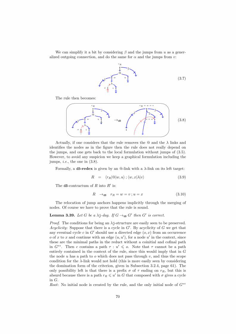
We can simplify it a bit by considering β and the jumps from u as a gener-alized outgoing connection, and do the same for α and the jumps from v:

rR

j

w u

@

vx

λ

j (3.7)

The rule then becomes:'

&

$

%

rR

j

w u

@

vx

λ

j →dB

rR = w = v

j

x = u

j j

(3.8)

Actually, if one considers that the rule removes the @ and the λ links andidentifies the nodes as in the figure then the rule does not really depend onthe jumps, and one gets back to the local formulation without jumps of (3.5).However, to avoid any suspicion we keep a graphical formulation including thejumps, i.e., the one in (3.8).

Formally, a dB-redex is given by an @-link with a λ-link on its left target:

R = 〈rR|@|w, u〉 ; 〈w, x|λ|v〉 (3.9)

The dB-contractum of R into R′ is:

R →dB rR = w = v ; u = x (3.10)

The relocation of jump anchors happens implicitly through the merging ofnodes. Of course we have to prove that the rule is sound.

Lemma 3.39. Let G be a λj-dag. If G→dB G′ then G′ is correct.

Proof. The conditions for being an λj-structure are easily seen to be preserved.Acyclicity : Suppose that there is a cycle in G′. By acyclicity of G we get thatany eventual cycle c in G′ should use a directed edge (o, x) from an occurrenceo of x to x and continue with an edge (u, u′), for a node u′ in the context, sincethese are the minimal paths in the reduct without a coinitial and cofinal pathin G∗∗. Then c contains a path τ : u′ 6 o. Note that τ cannot be a pathentirely contained in the context of the rule, since this would imply that in Gthe node u has a path to o which does not pass through v, and thus the scopecondition for the λ-link would not hold (this is more easily seen by consideringthe domination form of the criterion, given in Subsection 3.2.4, page 61). Theonly possibility left is that there is a prefix σ of τ ending on rR, but this isabsurd because there is a path rR 6 u′ in G that composed with σ gives a cyclein G.Root : No initial node is created by the rule, and the only initial node of G∗∗

70

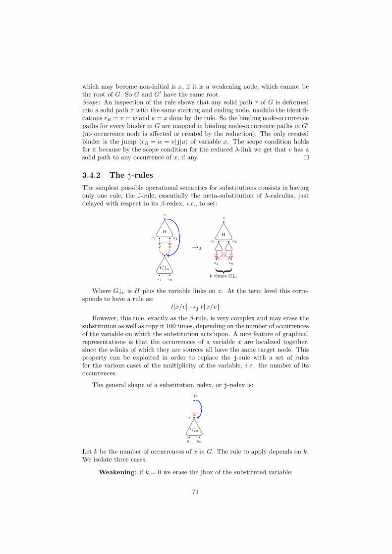
which may become non-initial is x, if it is a weakening node, which cannot bethe root of G. So G and G′ have the same root.Scope: An inspection of the rule shows that any solid path τ of G is deformedinto a solid path τ with the same starting and ending node, modulo the identifi-cations rR = v = w and u = x done by the rule. So the binding node-occurrencepaths for every binder in G are mapped in binding node-occurrence paths in G′

(no occurrence node is affected or created by the reduction). The only createdbinder is the jump 〈rR = w = v|j|u〉 of variable x. The scope condition holdsfor it because by the scope condition for the reduced λ-link we get that v has asolid path to any occurrence of x, if any.

3.4.2 The j-rules

The simplest possible operational semantics for substitutions consists in havingonly one rule, the J-rule, essentially the meta-substitution of λ-calculus, justdelayed with respect to its β-redex, i.e., to set:

v

H

o1 ok. . .

x

v v

G↓u

z1 zn

. . .

j

→J

v

H

o1 ok. . .

z1 znk times G↓v

. . .

Where G↓v is H plus the variable links on x. At the term level this corre-sponds to have a rule as:

t[x/v]→j tx/v

However, this rule, exactly as the β-rule, is very complex and may erase thesubstitution as well as copy it 100 times, depending on the number of occurrencesof the variable on which the substitution acts upon. A nice feature of graphicalrepresentations is that the occurrences of a variable x are localized together,since the v-links of which they are sources all have the same target node. Thisproperty can be exploited in order to replace the j-rule with a set of rulesfor the various cases of the multiplicity of the variable, i.e., the number of itsoccurrences.

The general shape of a substitution redex, or j-redex is:

rR

x

G↓x

y1 yn

. . .

j

Let k be the number of occurrences of x in G. The rule to apply depends on k.We isolate three cases:

Weakening: if k = 0 we erase the jbox of the substituted variable:

71

'

&

$

%

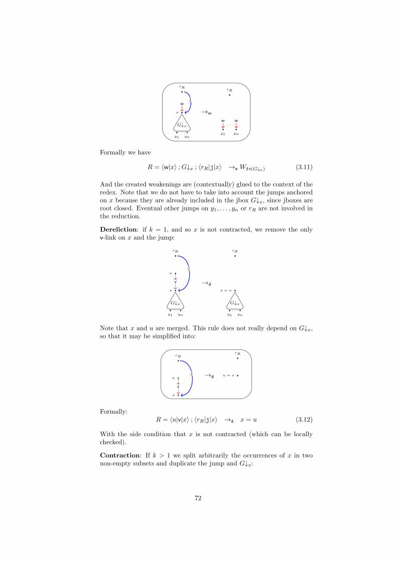
rR

x

w

G↓x

y1 yn

. . .

j

→w

rR

y1 yn

w w. . .

Formally we have

R = 〈w|x〉 ;G↓x ; 〈rR|j|x〉 →w Wfv(G↓x) (3.11)

And the created weakenings are (contextually) glued to the context of theredex. Note that we do not have to take into account the jumps anchoredon x because they are already included in the jbox G↓x, since jboxes areroot closed. Eventual other jumps on y1, . . . , yn or rR are not involved inthe reduction.

Dereliction: if k = 1, and so x is not contracted, we remove the onlyv-link on x and the jump:

rR

u

x

v

G↓x

y1 yn

. . .

j

→d

rR

u = x

G↓x

y1 yn

. . .

Note that x and u are merged. This rule does not really depend on G↓x,so that it may be simplified into:#

"

!

rR

u

x

v

j →d

rR

u = x

Formally:R = 〈u|v|x〉 ; 〈rR|j|x〉 →d x = u (3.12)

With the side condition that x is not contracted (which can be locallychecked).

Contraction: If k > 1 we split arbitrarily the occurrences of x in twonon-empty subsets and duplicate the jump and G↓x:

72

'

&

$

%

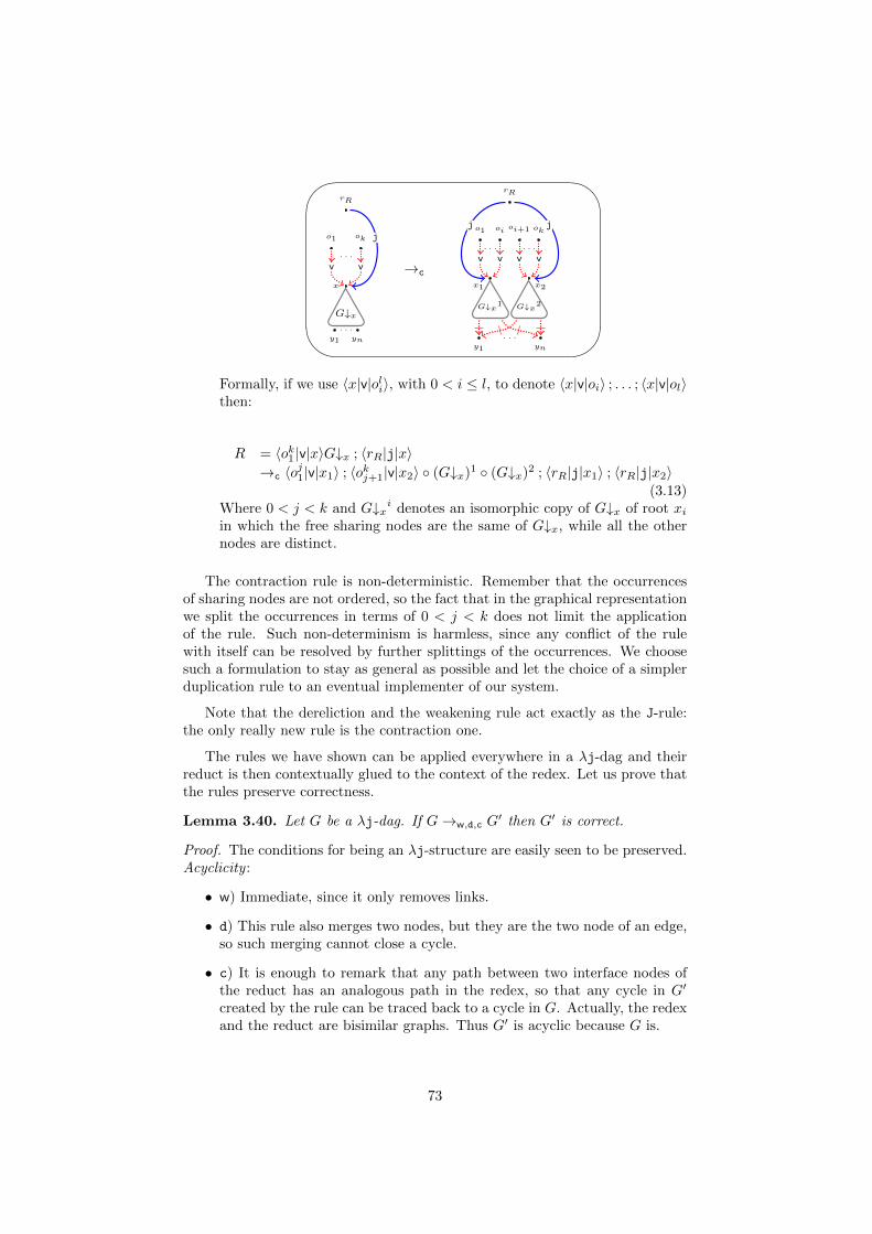
rR

o1 ok

. . .

x

v v

G↓x

y1 yn

. . .

j

→c

rR

o1 oi oi+1 ok

. . . . . .

x1

v v

x2

v v

G↓x1 G↓x2

y1 yn

. . .

jj

Formally, if we use 〈x|v|oli〉, with 0 < i ≤ l, to denote 〈x|v|oi〉 ; . . . ; 〈x|v|ol〉then:

R = 〈ok1 |v|x〉G↓x ; 〈rR|j|x〉→c 〈oj1|v|x1〉 ; 〈okj+1|v|x2〉 (G↓x)1 (G↓x)2 ; 〈rR|j|x1〉 ; 〈rR|j|x2〉

(3.13)Where 0 < j < k and G↓xi denotes an isomorphic copy of G↓x of root xiin which the free sharing nodes are the same of G↓x, while all the othernodes are distinct.

The contraction rule is non-deterministic. Remember that the occurrencesof sharing nodes are not ordered, so the fact that in the graphical representationwe split the occurrences in terms of 0 < j < k does not limit the applicationof the rule. Such non-determinism is harmless, since any conflict of the rulewith itself can be resolved by further splittings of the occurrences. We choosesuch a formulation to stay as general as possible and let the choice of a simplerduplication rule to an eventual implementer of our system.

Note that the dereliction and the weakening rule act exactly as the J-rule:the only really new rule is the contraction one.

The rules we have shown can be applied everywhere in a λj-dag and theirreduct is then contextually glued to the context of the redex. Let us prove thatthe rules preserve correctness.

Lemma 3.40. Let G be a λj-dag. If G→w,d,c G′ then G′ is correct.

Proof. The conditions for being an λj-structure are easily seen to be preserved.Acyclicity :

• w) Immediate, since it only removes links.

• d) This rule also merges two nodes, but they are the two node of an edge,so such merging cannot close a cycle.

• c) It is enough to remark that any path between two interface nodes ofthe reduct has an analogous path in the redex, so that any cycle in G′

created by the rule can be traced back to a cycle in G. Actually, the redexand the reduct are bisimilar graphs. Thus G′ is acyclic because G is.

73

Root : Note that rR is the source of a link, otherwise it could not be a subtermnode and the anchor of a jump, and so in the w, d-cases it does not becomean isolated node.

• w) If the rule creates an initial node it is one of the yi. Suppose that yiis an initial node in G′. If it is free or the variable node of a λ-link thenit induces an isolated initial node, which is harmless for correctness. If itis substituted then it is the anchor of a jump in G and so in G′, where itcannot be initial, absurd.

• d) If u = x is an entry node in G′ then it is an entry node in G, actuallythe root since it is the source of a link. No other node is affected by thereduction.

• c) Evident: no node looses its incoming connection and no entry nodegets them.

Scope: the binders of G affected by the rule are all and only those having a pathτ from their binding node u to one of their occurrences o passing through thereduced jump j. Since jboxes are closed by solid path suffixes o is in G↓x andthus it is an occurrence of a free variable of G↓x. Any solid path not using thereduced jump is not affected by the rule, since jboxes are internally closed.

• w) The rule erases the solid path τ together with the occurrence o, andthere is nothing left to prove for o in G′.

• d) τ has an analogous coinitial and cofinal path τ ′ in G′ obtained bysubstituting j in τ with the solid path from rR to u, existing by the scopecondition for j.

• c) For any duplicated occurrence of a free variable yi of G↓x the rule alsoduplicates the solid path from rR to it.

Now let us explain the argument showing that the critical pair generated bythe c-rule with itself on a given contraction redex can be closed.

Two applications of the rule corresponds to two bipartitions (O1, O2) and(O3, O4) of the set of occurrences O of x (with |O| > 1) s. t. any Oi fori = 1, 2, 3, 4 is non-empty and different from O. Consider the four intersectionsOij := Oi ∩ Oj for i = 1, 2 and j = 3, 4. Let us prove that (O1, O2) reduces tothe 4-partition (O13, O14, O23, O24) by further bipartitions. If O1 = O13 thenO14 = ∅ and no action on O1 is needed. If O13 ⊂ O1 then simply split O1 in O13

and O14. Similarly for O2, and for (O3, O4). So in at most 2 c-steps (at mostone for O1 and at most one for O2) we get (O1, O2)→∗c (O13, O14, O23, O24) andin the same number of steps (O3, O4)→∗c (O13, O14, O23, O24), so we conclude.

3.5 Terms, graphs and strong bisimulations

Often a graph formalism is seen as a useful implementation allowing some formof sharing for a sequential language where there is no primitive notion of sharing.In our case the sequential language is the λ-calculus and the graphical one is

74

given by λj-dags. To show the correctness of the implementation it is necessaryto show that any single step in the sequential system, i.e., a β-reduction, can besimulated by the graphs. In general in the graphical system a rewriting step ofthe sequential language is simulated through a sequence of steps. For instance,given an ordinary λ-term t the simulation on λj-dags has the following shape:

t →β t′

↓· ↓·t →+ t′

The other direction is more delicate, since a step in the graphical languageusually corresponds only to a fragment of a sequential step. For instance givena reduction from t the situation would be:

t → t′

t → G′ ⇒ ↓· ↓·t → G′ →∗ t′

Put differently, to relate the two reductions it is necessary to complete thegraphical step into a reduction sequence representing a sequential step.

But this is the easy case, since we assumed to have a graph t, which is thetranslation of a λ-term. Reductions on an arbitrary given (correct) graph G aremore complicated to project on terms because there may be no ordinary λ-termtranslating to G, if G presents some sharing. Thus a reduction G → G′ has tobe first projected on a graph H without sharing. But if the redex of G is in ashared part then the step in G can correspond to the reduction of many redexesin H and thus on the corresponding term, or eventually to nothing at all, if theshared part is erased by the projection.

One of the cornerstones of our approach is to avoid such complex relationbetween terms and graphs by using a richer term language, where sharing isvisible, i.e., using terms with explicit substitutions (ES, for short), so that agraph G can always be seen as a term. Note, however, that we did not defineany rewriting rule on λj-terms.

The problem is that there is no canonical calculus of explicit substitutions(see Section 4.1, page 88, for an introduction to explicit substitutions), so it isnot clear which calculus should be related to λj-dags, once the term languagehas been enriched.

But we have developed a powerful tool: the read-back. The idea is thatwe can bypass the usual proof of soundness of our system, going the other wayaround and complete the following diagram:

G → G′

↓· ↓·t t′

(3.14)

Where t is a read-back of G and t′ a read-back of G′ by defining on λj-terms arule of the form:

t→ t′

The outcome is an operational semantics on λj-terms which is the exact copyof the λj-dags semantics. The soundness of the implementation of the obtained

75

calculus with respect to λj-dags then holds by construction. Soundness withrespect to the λ-calculus can be proved by relating the extracted ES-calculuswith λ-calculus, which is a simpler task since λ-terms are λj-terms, and weshould not pass through the read-back.

Let us make a technical observation. Note that a given λj-dag can havemore than one read-back so that if we require that diagram (3.14) is valid forany read-back of G and G′ then we have to define the reduction on λj-termsmodulo the quotient ≡CS induced by the translation. However, the idea can be

refined so that there is no need of the modulo. Given a read-back t = G4

wecan define the term rule t → t′ with respect to a particular read-back of G′

depending on 4. In this way we get a calculus which makes sense without anyprimitive congruence.

In the next section we shall pull-back the operational semantics of λj-dags onλj-terms, following this principle. The presented methodology has the followingadvantages:

• We get a perfect bidirectional one-step-to-one-step relation between theextracted calculus and λj-dags. Then results for the calculus very easilytransfer to λj-dags, and viceversa.

• We can contribute to the quest of a canonical explicit substitution calculus,by exploiting the relation with the graphs and the underlying Linear Logicdynamics.

• We can use the techniques developed in 20 years of research on explicitsubstitutions to study the calculus arising from λj-dags, in particular wecan easily relate it to the λ-calculus.

Let us now discuss the precise form of relation we want to establish betweenλj-dags and the calculus we want to extract. The idea is to define on λj-termsfour rules corresponding to the dB, w, d, c-rules of λj-dags so that we get thefollowing diagrams:

G →x G′ G →x G′

↓· ⇒ ∃ t′ s.t. ↓· ↓·t t →x t′

For x ∈ dB, w, d, c, and

G G →x G′

↓· ⇒ ∃ G′ s.t. ↓· ↓·t →x t′ t →x t′

This amounts to say that the read-back is a strong bisimulation betweenλj-terms and λj-dags. For the definition of strong bisimulation see definition2.28 (page 39).

Of course, this implies that the translation is a strong bisimulation too, sinceit inverts the read-back.

Termination is a strong bisimulation invariant: if R is a strong bisimulationbetween two rewriting systems X and Y then a term x ∈ X s.t. xRy for y ∈ Y

76

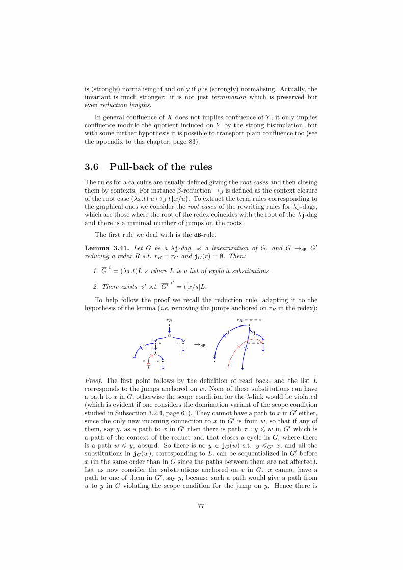
is (strongly) normalising if and only if y is (strongly) normalising. Actually, theinvariant is much stronger: it is not just termination which is preserved buteven reduction lengths.

In general confluence of X does not implies confluence of Y , it only impliesconfluence modulo the quotient induced on Y by the strong bisimulation, butwith some further hypothesis it is possible to transport plain confluence too (seethe appendix to this chapter, page 83).

3.6 Pull-back of the rules

The rules for a calculus are usually defined giving the root cases and then closingthem by contexts. For instance β-reduction→β is defined as the context closureof the root case (λx.t) u 7→β tx/u. To extract the term rules corresponding tothe graphical ones we consider the root cases of the rewriting rules for λj-dags,which are those where the root of the redex coincides with the root of the λj-dagand there is a minimal number of jumps on the roots.

The first rule we deal with is the dB-rule.

Lemma 3.41. Let G be a λj-dag, 4 a linearization of G, and G →dB G′

reducing a redex R s.t. rR = rG and jG(r) = ∅. Then:

1. G4

= (λx.t)L s where L is a list of explicit substitutions.

2. There exists 4′ s.t. G′4′

= t[x/s]L.

To help follow the proof we recall the reduction rule, adapting it to thehypothesis of the lemma (i.e. removing the jumps anchored on rR in the redex):

rR

w u

@

vx

λ

j →dB

rR = w = v

x = u

j j

Proof. The first point follows by the definition of read back, and the list Lcorresponds to the jumps anchored on w. None of these substitutions can havea path to x in G, otherwise the scope condition for the λ-link would be violated(which is evident if one considers the domination variant of the scope conditionstudied in Subsection 3.2.4, page 61). They cannot have a path to x in G′ either,since the only new incoming connection to x in G′ is from w, so that if any ofthem, say y, as a path to x in G′ then there is path τ : y 6 w in G′ which isa path of the context of the reduct and that closes a cycle in G, where thereis a path w 6 y, absurd. So there is no y ∈ jG(w) s.t. y 6G′ x, and all thesubstitutions in jG(w), corresponding to L, can be sequentialized in G′ beforex (in the same order than in G since the paths between them are not affected).Let us now consider the substitutions anchored on v in G. x cannot have apath to one of them in G′, say y, because such a path would give a path fromu to y in G violating the scope condition for the jump on y. Hence there is

77

no y ∈ jG(v) s.t. x 6G′ y, i.e., x is maximal in the λj-dag G′′ obtained fromG′ after the removal of the substitutions in L and can be removed. After theseremovals we are left with a λj-dag G′′′ which is exactly G↓v 〈w|x〉, i.e., thesubdag of G reading back to t (using the restriction of 4). So G′ reads back tot[x/s]L.

It is easy to see that G′ can also be read-back as tL[x/s]: the created sub-stitution [x/s] is actually independent from the substitutions in L, so that itis possible to sequentialize [x/s] anywhere in the middle of L, too. If [x/s] issequentialized before or after L does not matter: it is important, however, tofix one way of sequentializing and then stick to it.

For the j-rules, analogously, we deal with a root case. But let us firstintroduce some notations, formally.

Definition 3.42. If t is a λj-term and x is a variable we use |t|x for the numberof occurrences of x in t, defined by induction on the α-equivalence class of tas follows:

|x|x = 1|y|x = 0|λy.t|x = |t|x|t v|x = |t|x + |v|x|t [y/v]|x = |t|x + |v|x

The next notion is used to describe on terms the action of the contractionrule on λj-dags.

Definition 3.43. Let t be a λj-term, x ∈ fv(t) and y /∈ fv(t). The non-deterministic replacement of y to x in t is a term t<y>x defined by inductionon the α-equivalence class of t as follows:

x<y>x ∈ x, yz<y>x = z(λz.t)<y>x = λz.t<y>x(t v)<y>x = t<y>x v<y>x(t [z/v])<y>x = t<y>x v<y>x

Consider the following terms:

t1 = z x x x xt2 = z y x x xt3 = z y x y xt4 = z y y x yt5 = z y y y yt6 = y x x x x

(3.15)

They are all non-deterministic replacements of y to x in z x x x x (or, simmet-rically, of x to y in z y y y y) except t6.

Definition 3.44 (variable splitting t[y]x). If |t|x > 1 an y-splitting t[y]x of xin t is a non-deterministic replacement t′ = t<y>x of y to x in t s.t. |t′|x ≥ 1and |t′|y ≥ 1.

78

Put differently the notation t[y]x means that a non-empty proper subset ofthe occurrences of x in t has been renamed y, if |t|x ≥ 2. Among the terms in(3.15) only t2, t3 and t4 are y-splitting of x in z x x x x.

Lemma 3.45. Let G be a λj-dag with a j-redex R of substitution node x androot node the root of G (i.e. rR = rG), 4 a linearization of G s.t. x is the

maximum of 4rG , and let G′ be G after the contraction of R. Then G4

= t[x/s]and:

1. If G→w G′ there exists 4′ s.t. G′

4′= t.

2. If G→d G′ there exists 4′ s.t. G′

4′= tx/s.

3. If G→c G′ there exists 4′ s.t. G′

4′= t[y]x [x/s][y/s].

Proof. The substitution x is maximal in j(r), since 4r extends 6r. The substi-tution splitting lemma give us G = (G6↑x G↓x) ; 〈r|j|x〉. Then by definition of

read-back we get G4

= t[x/s], where t = G6↑x4

and s = G↓x4

.G→w G

′) The reduction is:

G→w (G6↑x Wfv(G↓x)) = G′

Thus G′ is G6↑x modulo some free weakenings, and they have the same readbacks, since the read-back does not depend on free weakenings, in particular t.G→d G

′) The idea is that the read back of G′ is nothing else than the one of twhere the read back of the only v-link on x is replaced by the read back of G↓x,which gives the statement. Formally it is proved by induction on G6↑x (i.e. byinduction on t).G→c G

′) The two new substitutions of G′ are mutually independent and max-imal in G′ since x is maximal in G. Then, if the two nodes in which x is splittedare named x and y then we get a term t′[x/s][y/s]. The λj-dag K ′ = G↓rR 6↑xreading back to t and K ′ = G′ 6↑x 6↑y reading back to t′ only differ for the factthat x and y are contracted in K while they are not in K ′. The only part of theread-back which depends on which free v-links are contracted together is thenaming of free occurrences for the read-back term. So t′ is t where some (andnot all) occurrences of x have been renamed y, i.e., t′ = t[y]x .

We can finally define the operational semantics of our calculus of explicitsubstitutions.

Definition 3.46 (structural λ-calculus). The structural λ-calculus λj isgiven by the language of λj-terms and by the following root rules:

(dB) (λx.t)L u 7→dB t[x/u]L(w) t[x/u] 7→w t if |t|x = 0(d) t[x/u] 7→d tx/u if |t|x = 1(c) t[x/u] 7→c t[y]x [x/u][y/u] if |t|x > 1

We recall that t[x/u] binds x in t, i.e., that fv(t[x/u]) = (fv(t)\x)∪fv(u).

We close these rules by contexts, as usual: →a denotes the contextual closureof 7→a, for a ∈ dB,w, d, c.

To prove that the structural λ-calculus is strongly bisimilar to λj-dags weneed the two following simple facts.

79

Lemma 3.47. Let t be a λj-term and y ∈ fv(t). Then the free sharing node oftX corresponding to y has |t|y occurrences in tX .

Proof. Straightforward induction on the translation.

Lemma 3.48. Let G be a λj-dag, R a redex of G of root rR. Then R iscontained in G↓rR .

Proof. For the dB-redexes it is immediate, since any involved link has a pathfrom rR. In the case of a w, d, c-redex on a jump j it follows by root closureof G↓rR , which forces j and the jbox of its target to be part of G↓rR , and thescope condition for j, which implies that the v-links on the target of the jumpare in G↓rR .

As expected we get:

Theorem 3.49 (strong bisimulation). The read-back is a full strong bisimula-tion between λj-dags and the structural λ-calculus. Explicitly: let G be a λj-dag

and t = G4

one of its read-backs. For a ∈ dB, w, d, c

1. If G→a G′ then there exists t′ s.t. t→a t

′ and G′ RB t′.

2. If t→a t′ then there exists a unique G′ s.t. G→a G

′ and G′ RB t′.

Proof. By induction on the read-back t = G4

. It is an almost immediateconsequence of the pull-back lemmas.Suppose that the root r of G is the anchor of some jumps. Then let j = 〈r|j|x〉be the maximum jump with respect to 4. We get t = s[x/v] where s = G6↑x

4

and v = G↓x4

(remember that if H is a subdag of G and G4

is a read-back of

G we use H4

to denote the read-back of H obtained by restricting 4 to H). Byi.h. the read-back is a full strong bisimulation between s and G6↑x, and betweenv and G↓x, satisfying the statement.Consider the redex R given by j and the reduct G′ of G after the reductionof R: we have G →a G

′ with a ∈ w, d, c. By lemma 3.45 there exist t′ s.t.t→a t

′ by reducing the redex on [x/v] and G′ RB t′. Suppose now that t→a t′.

By lemma 3.47 we get that x has the same number of occurrences in G6↑x and s.If a ∈ w, d then the reduction of R in G and lemma 3.45 give a term t′′ s. t.t→a t

′′ by reducing [x/v]: these reductions are deterministic so t′ = t′′ and weconclude. If a = c then s[x/v] 7→c s[y]x [x/v][y/v] = t′ for a certain y-splitting ofx in t. Let S be the set of occurrences of x in G corresponding to those renamedas y in s[y]x and G′ the reduct of G obtained by the contraction step on x whichseparates the occurrences in S from the other occurrences of x. G′ reads-backto t′ by lemma 3.45.Suppose that there is a redex R′ of G which is not contained in G6↑x nor in G↓x,which are disjoint sets of link by definition of G6↑x. It cannot be a dB-redex,since its root node rR′ must belong either to G↓x or G6↑x, and it is readily seenthat this would imply R′ ⊆ G6↑x or R′ ⊆ G↓x (because any link involved ina dB-redex R′ has a path from rR′), absurd. Then R′ is a substitution redexconcerning a variable y. Since any substituted sharing node y 6= x of G is asubstituted sharing node in either G6↑x or G↓x then we get R′ = R. Similarlythe only redex of s[x/v] not in s or in v is the one given by [x/v].Let us discuss a case of inductive reduction. Let G →a G′ be a reduction

80

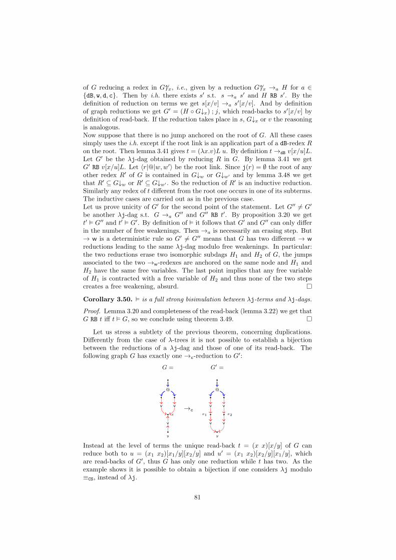
of G reducing a redex in G 6↑x, i.e., given by a reduction G6↑x →a H for a ∈dB, w, d, c. Then by i.h. there exists s′ s.t. s →a s

′ and H RB s′. By thedefinition of reduction on terms we get s[x/v] →a s

′[x/v]. And by definitionof graph reductions we get G′ = (H G↓x) ; j, which read-backs to s′[x/v] bydefinition of read-back. If the reduction takes place in s, G↓x or v the reasoningis analogous.Now suppose that there is no jump anchored on the root of G. All these casessimply uses the i.h. except if the root link is an application part of a dB-redex Ron the root. Then lemma 3.41 gives t = (λx.v)L u. By definition t→dB v[x/u]L.Let G′ be the λj-dag obtained by reducing R in G. By lemma 3.41 we getG′ RB v[x/u]L. Let 〈r|@|w,w′〉 be the root link. Since j(r) = ∅ the root of anyother redex R′ of G is contained in G↓w or G↓w′ and by lemma 3.48 we getthat R′ ⊆ G↓w or R′ ⊆ G↓w′ . So the reduction of R′ is an inductive reduction.Similarly any redex of t different from the root one occurs in one of its subterms.The inductive cases are carried out as in the previous case.Let us prove unicity of G′ for the second point of the statement. Let G′′ 6= G′

be another λj-dag s.t. G →a G′′ and G′′ RB t′. By proposition 3.20 we get

t′ G′′ and t′ G′. By definition of it follows that G′ and G′′ can only differin the number of free weakenings. Then →a is necessarily an erasing step. But→ w is a deterministic rule so G′ 6= G′′ means that G has two different → wreductions leading to the same λj-dag modulo free weakenings. In particular:the two reductions erase two isomorphic subdags H1 and H2 of G, the jumpsassociated to the two →w-redexes are anchored on the same node and H1 andH2 have the same free variables. The last point implies that any free variableof H1 is contracted with a free variable of H2 and thus none of the two stepscreates a free weakening, absurd.

Corollary 3.50. is a full strong bisimulation between λj-terms and λj-dags.

Proof. Lemma 3.20 and completeness of the read-back (lemma 3.22) we get thatG RB t iff t G, so we conclude using theorem 3.49.

Let us stress a subtlety of the previous theorem, concerning duplications.Differently from the case of λ-trees it is not possible to establish a bijectionbetween the reductions of a λj-dag and those of one of its read-back. Thefollowing graph G has exactly one →c-reduction to G′:

G = G′ =

@

x

v v

y

v

→c

@

x1 x2

v v

y

v v

Instead at the level of terms the unique read-back t = (x x)[x/y] of G canreduce both to u = (x1 x2)[x1/y][x2/y] and u′ = (x1 x2)[x2/y][x1/y], whichare read-backs of G′, thus G has only one reduction while t has two. As theexample shows it is possible to obtain a bijection if one considers λj modulo≡CS, instead of λj.

81

It is natural to observe that the real algebraic form of λj-dags is given byλj modulo ≡CS and not by λj. This is certainly true, but avoiding ≡CS weshowed a strong and non-trivial property which might have been hidden by thetechnical development: the sequentialization of a λj-dag can be preserved byreduction. The use of linearizations is the key technical notion for getting suchresult. Moreover, we believe that a calculus without any primitive congruenceis easier to study and divulge.

A graphical representation does not necessarily enjoy the fact that the reduc-tion can be transported on terms preserving the sequentialization. For instance,the experimental syntax of Chapter 7 does not, as it is shown by the exampleat the end of that chapter.

But let us consider λj modulo ≡CS. As a by-product of our construction,based on relating terms and graphs through a strong bisimulation, we can provethat ≡CS is extremely well-behaved: we can compose the quotient induced bythe translation with the strong bisimulation and get that ≡CS is an internalstrong bisimulation on λj-terms, i.e., a bisimulation of λj within itself (whichis not the identity!).

Corollary 3.51. ≡CS is a strong bisimulation over λj-terms.

Proof. If t ≡CS t′ we get from theorem 3.37 G = t = t′. If t →a s, witha ∈ dB, w, d, c, then by Corollary 3.50 G →a H and s ` H. Applying thecorollary to G and t′ we get t′ →a s

′ and s′ H. Then s and s′ both translatesto H and theorem 3.37 gets s ≡CS s

′. Analogously if the reduction takes placein t′.

In the next chapter we shall prove confluence of the structural λ-calculus(theorem 4.22). From that and Corollary 3.51 we shall get that λj is evenChurch-Rosser modulo ≡CS (property defined at page 86), which is the strongestform of confluence property for a rewriting system modulo an equivalence rela-tion (lemma 4.24, page 103).

Traditional calculi of explicit substitutions often employ ≡CS to recover someoperational properties (see the introduction to the next chapter). But in thesecases ≡CS is not a strong bisimulation. This point is interesting: in these calculi≡CS:

M [x/s][y/v] ∼CS M [y/v][x/s] when x /∈ fv(v) and y /∈ fv(s)

Is needed to reveal a redex for [y/v] otherwise hidden by [x/s]. This means thatusually ≡CS creates redexes. If a relation creates redexes in general it is not astrong bisimulation.

3.6.1 Milner’s rules

In [Mil07] Robin Milner introduces a λ-calculus with explicit substitutions in-spired by his translation of λ-calculus into Bigraphs, a graphical formalisms hedeveloped. Such calculus is strikingly similar to ours, despite having been de-veloped independently, but there are subtle differences. The rules of Milner’scalculus λm are:

82

(dBm) (λx.t) u →dBm t[x/u](dm) C[x][x/u] →dm C[u][x/u](wm) t[x/u] →wm t if x /∈ fv(t)

Where C[·] is a context which does not bind x. His→dBm is the typical B-rulereplacing β in almost all explicit substitution calculi. It may be implemented inλj-dags defining a graphical dB-redex as we have done but it requires to imposethat no jump is anchored on the source of the λ-link. However, this constraintis in general too strong, since there is a quotients of λj-dags, given by Regnier’sPure Proof Nets see Chapter 5, where such constraint cannot be formulated.

The main difference in the substitutions rules is that λm makes a copy evenwhen there is only one occurrence of the substitution. Indeed, we get thatx[x/y] →dm y[x/y] →wm y whereas in λj we would have x[x/y] →d y, avoidinga useless duplication. The last less relevant difference is that duplications areperformed isolating at each step one occurrence and immediately substitutingupon it, while in λj there is a neat separation between the duplication process,which may split occurrences in a much more general way, and the substitution.While →wm is exactly ours →w, the rule →dm cannot always be simulated byour system, because of the duplication in absence of occurrences, so it needs anew graphical rule. In Figure 3.2 there are the λj-dags rules for representingλm, where we have suggested some of the subterms (G↓u and G↓v in dBm and Hin dm) to make the rules more readable, despite they are not really part of theredex. In the →dm rule o1 has to be understood as no matter which occurrenceof x, not necessarily the leftmost. Moreover in the case where k = 1 the reductintroduces a weakening on R↓x2. It is more or less immediate to see that theypreserve correctness, and one easily gets a strong bisimulation between λm andλj-dags with respect to this different operational semantics, following the linesof what we did for λj.

Along our study of λj we shall see that the apparent slight operationaldifferences between λj and λm are crucial, and that various results we will obtainfor λj would not be possible using λm.

3.7 Appendix: strong bisimulations

We show some easy facts on the preservation of operational properties by strongbisimulation which are used in the following chapters. First of all we recall thedefinition.

Definition 3.52 (strong bisimulation). Let (X,→) and (Y, ) two rewritingsystems, with reduction steps labelled from a common set L. A strong bisim-ulation between X and Y is a relation ≡ between terms of X and terms of Ys.t. if x ≡ y, with x ∈ S and y ∈ Q, then for a ∈ L:

1. If x→a x′ then y a y

′ and x′ ≡ y′, and conversely

2. If y a y′ then x→a x

′ and x′ ≡ y′.

A strong bisimulation is full if

• for every x ∈ X there exists y ∈ Y s.t. x ≡ y, and

83

'

&

$

%

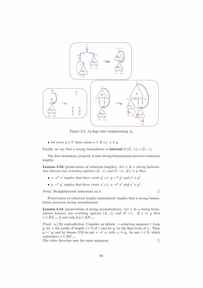
r

w u

@

R↓u

z1 zn

. . .v

R↓v

x

λ →dBm

v = r

R↓v

x

R↓u

z1 zn

. . .

j

'

&

$

%

rR

x

w

G↓x

y1 yn

. . .

j

→w

rR

y1 yn

w w. . .

'

&

$

%

v

H

o1 ok. . .

x

v v

R↓x

z1 zn

. . .

j

7→dm

v

H

o1 o2 ok. . .

x2

v vR↓x1

R↓x2z1

zn

. . .

j

Figure 3.2: λj-dags rules implementing λm

• for every y ∈ Y there exists x ∈ X s.t. x ≡ y.

Finally, we say that a strong bisimulation is internal if (X,→) = (Y, ).

The first elementary property is that strong bisimulations preserve reductionlengths.

Lemma 3.53 (preservation of reduction lengths). Let ≡ be a strong bisimula-tion between two rewriting systems (X,→) and (Y, ). If x ≡ y then

• x→k x′ implies that there exists y′ s.t. y k y′ and x′ ≡ y′.

• y k y′ implies that there exists x′ s.t. x→k x′ and x′ ≡ y′.

Proof. Straightforward inductions on k.

Preservation of reduction lengths immediately implies that a strong bisimu-lation preserves strong normalization.

Lemma 3.54 (preservation of strong normalization). Let ≡ be a strong bisim-ulation between two rewriting systems (X,→) and (Y, ). If x ≡ y thenx ∈ SN→ if and only if y ∈ SN .

Proof. ⇒) By contradiction. Consider an infinite -reduction sequence τ fromy, let τi the prefix of length i ∈ N of τ and let yi be the final term of τi. Theny i yi and by lemma 3.53 we get x →i xi with xi ≡ yi, for any i ∈ N, whichcontradicts x ∈ SN→.The other direction uses the same argument.

84

Now we turn to the study of how confluence is transported by strong bisim-ulations. Let ≡ be a full strong bisimulation between (X,→) and (Y, ). Ingeneral full strong bisimulations do not transport confluence diagrams, sincethey transport the two sides of a diagram, but they do not guarantee that thetwo final terms are equal. Take a confluence diagram in X, i.e., let x, x1, x2, x

′

be s.t.

x→ xi and xi →∗ x′, for i = 1 and i = 2

Then ≡ gives us terms y, y1, y2, y′1, y′2 s.t. x ≡ y, xi ≡ yi x

′ ≡ y′i, for i = 1and i = 2, and:

y ∗ yi and yi ∗ y′i, for i = 1 and i = 2

But in general y′1 6= y′2, and so we cannot infer confluence of (Y, ). However,it is possible to infer confluence of Y modulo the quotient induced by ≡ on Y .

Define ≡Y as the relation on Y s.t. y ≡Y y′ if there exists x s.t. x ≡ y andx ≡ y′. It is immediate that ≡Y is an equivalence relation. In general one canonly prove that confluence of → implies confluence of modulo ≡Y .

Lemma 3.55 (confluence to confluence modulo). Let ≡ a full strong bisimula-tion between two rewriting systems (X,→) and (Y, ). If → is confluent then is confluent modulo ≡Y .

Proof. Let y, y′ ∈ Y s.t. y ≡Y y′, y ∗ y1 and y′ ∗ y2. Since y ≡Y y′ we getthat there exists x s.t. x ≡ y and x ≡ y′ (in the case y = y′ we still get thatsuch an x exists, since ≡ is full). By strong bisimulation x→∗ xi with xi ≡ yi,for i = 1, 2. Since → is confluent there exists x′ s.t. xi →∗ x′. By lemma 3.53there exists y3 and y4 s.t. y1 ∗ y3 and y2 ∗ y4 with x′ ≡ y3 and x′ ≡ y4. Bydefinition y3 ≡Y y4 so we conclude.

However, it is possible to improve and transport plain confluence to plainconfluence adding some hypothesis on ≡.

It would be enough that ≡, when considered from X to Y , is a functionso that we get that ≡Y is the identity and enjoys plain confluence (by theprevious lemma, since a reduction relation modulo the identity is the reductionitself). Unfortunately, in general the strong bisimulations we use in this thesis(the translation modulo weakenings and the read-back) are not functions. Inparticular is not a function from λj-terms to λj-dags because it is defined asthe translation modulo free weakenings2).

Still, we shall transport confluence from λj-terms to λj-dags. Indeed, aweaker hypothesis on how the strong bisimulation relates to (X,→) guaranteesthat confluence of X maps to plain confluence of Y , as the next lemma shows.And enjoys this property.

Lemma 3.56 (confluence to confluence). Let ≡ a full strong bisimulation be-tween two rewriting systems (X,→) and (Y, ). If for every x ∈ X, for everyreduction x→a x

′ of label a and for every y s.t. x ≡ y there exists a unique y′

s.t. y a y′ and x′ ≡ y′ then

2It is necessary to use and not the translation in the empty context, since weakeningrewriting steps create free weakenings on λj-dags which have no analogous on terms, and sowithout reasoning modulo free weakenings the strong bisimulation does not hold.

85

1. Whenever x ≡ y and x →∗ x′ then there is a unique y′ s.t. y ∗ y′ andx′ ≡ y′.

2. → confluent implies confluent.

Proof. 1) Straightforward induction on the length of the reduction using thehypothesis.2) Let y ∈ Y and y ∗ yi with i ∈ 1, 2. Since ≡ is full we get that thereexists x s.t. x ≡ y and by strong bisimulation x →∗ xi with xi ≡ yi. Since →is confluent there exists x′ s.t. xi →∗ x′. By lemma 3.53 there exists y3 andy4 s.t. y1 ∗ y3 and y2 ∗ y4 with x′ ≡ y3 and x′ ≡ y4. By point 1 we gety3 = y4.

The next subsection studies the particular case of strong bisimulations ofa system (X,→) with respect to itself. These bisimulations naturally arise asthe quotient of the translation from (X,→) to another system (Y, ), wheneversuch translation is a strong bisimulation.

3.7.1 Internal strong bisimulation

Whenever a rewriting system (X,→) enjoys an internal strong bisimulation ≡which is an equivalence relation then rewriting modulo ≡ is particularly well-behaved. We use →≡ for ≡→≡. We first show that ≡ can be postponed.

Lemma 3.57 (≡ postponement). Let (X,→) be a rewriting system, ≡ an in-ternal strong bisimulation of (X,→) which is an equivalence relation and t ∈ X.If t→k

≡ t′ then t→k≡ t′.

Proof. By induction on k. If k = 1 then t ≡ u → u′ ≡ t′. By definition of≡ we get that if t ≡ u → u′ then there exists v s.t. t → v ≡ u′ and weconclude. If k > 1 then t →k−1

≡ u →≡ t′. By i.h. we get t →k−1 v ≡ u andu→ u′ ≡ t′. Then v ≡ u→ u′ becomes v → v′ ≡ u′ and we conclude, since weget t→k−1 v → v′ ≡ u′ ≡ t′.

The postponement implies that strong normalization lifts from → to →≡.

Corollary 3.58 (SN→ to SN→/≡). Let (X,→) be a rewriting system, ≡ aninternal strong bisimulation of (X,→), t ∈ X. Then t ∈ SN→ iff t ∈ SN→≡ .

Proof. ⇒) Consider an infinite→≡-reduction sequence τ from t, let τi the prefixof length i ∈ N of τ and let ti be the result of τi. Then t→i

≡ ti and by lemma3.57 we get t→i t′i ≡ ti. Thus for any i ∈ N t→i ti, against hypothesis.⇐) Obvious.

Now let us discuss confluence modulo. If rewriting is not consider moduloan equivalence relation being confluent and being Church-Rosser are equivalentproperties. Switching to rewriting modulo it is no longer the case: Church-Rosser modulo is a stronger property than confluence modulo.

Definition 3.59. Let (X,→) a rewriting system and ∼ an equivalence relationon X.

• → is confluent if ∗←→∗⊆→∗ ∗←.

86

• → is Church-Rosser if ↔⊆→∗ ∗← where ↔:= (→ ∪ ←)∗.

• → is confluent modulo ∼ if ∗← ∼→∗⊆ (→∗) ∼ (∗←).

• → is Church-Rosser modulo ∼ if↔∼⊆ (→∗) ∼ (∗←) where↔∼:= (→∪ ← ∪ ∼)∗.

The typical counter-example showing that Church-Rosser modulo is strongerthan confluence modulo is:

∼ ∼

Where→ is confluent modulo ∼ but not Church-Rosser modulo ∼ (considerthe rightmost and the leftmost nodes).

We can prove that confluence of→ implies that→ is Church-Rosser modulo≡, if ≡ is a strong bisimulation.

Lemma 3.60. Let (X,→) be a rewriting system, ≡ an internal strong bisim-ulation of (X,→) which is an equivalence relation and t ∈ X. If t ↔≡ t′ thent↔≡ t′.

Proof. By induction on k, where t(→ ∪ ← ∪ ≡)kt′. If k = 1 then there isnothing to prove. If k > 1 then t(→ ∪ ← ∪ ≡)k−1u(→ ∪ ← ∪ ≡)t′. Then byi.h. t↔ u′ ≡ u. By cases on u(→ ∪ ← ∪ ≡)t′:

• u← t′: then u′ ≡ u← t′ and so by strong bisimulation u′ ←≡ t′, and weget t↔ u′ ←≡ t′, i.e., t↔≡ t′.

• u→ t′: then u′ ≡ u→ t′ and so by strong bisimulation u′ →≡ t′, and weget t↔ u′ →≡ t′, i.e., t↔≡ t′.

Corollary 3.61. Let (X,→) be a rewriting system, ≡ an internal strong bisim-ulation of (X,→) which is an equivalence relation. If → is confluent then it isChurch-Rosser modulo ≡.

Proof. Let t ∈ X and t↔≡ t′. Then by the previous lemma we get t↔ u ≡ t′

for a certain u ∈ X. But → is Church-Rosser so there exists v s.t. t→∗ v andu→∗ v. Then by strong bisimulation t′ →∗≡ v and so we conclude.

87

Chapter 4

The structural λ-calculus

In this chapter we study the structural λ-calculus extracted by read-back fromλj-dags. We show that it is a very well-behaved calculus of explicit substitu-tions, enjoying all the sanity properties of such calculi.

In order to better appreciate the original novelties of this system we startby introducing some calculi of explicit substitutions. Then we show:

• Every λj-term t[x/u] can be reduced to tx/v, a property known as fullcomposition

• The reduction of the substitution subcalculus terminates.

• λj is confluent.

• λj preserves β-strong normalization.

All the these properties immediately transfer to λj-dags, through the strongbisimulation between λj-calculus and λj-dags.

We also show an application of λj: we shall give new operational charac-terizations of the result of a full-development and a full-superdevelopment ofa λ-term. This analysis will lead us to introduce an extended and new notionof development, the XL-development, whose possibility is disclosed by the finerules of λj.

All the results of this chapter have been developed in collaboration withDelia Kesner and have been published in [AK10].

4.1 Introduction to explicit substitutions

The research field about explicit substitution calculi born officially with thepaper Explicit Substitutions of Abadi, Cardelli, Curien and Levy [ACCL91].Their motivation was very well expressed in the introduction of that paper (ofwhich we have slightly changed the notation):

Substitution is the eminence grise of the λ-calculus. The classicalrule,

(λx.t) u →β tx/u

88

uses substitution crucially though informally. Here t and u denotetwo terms, and tx/u represents the term t where all free occur-rences of x are replaced with u. This substitution does not belongin the calculus proper, but rather in an informal meta-level. Similarsituations arise in dealing with all binding constructs, from universalquantifiers to type abstractions.A naive reading of the rule suggests that the substitution of u forx should happen at once, when the rule is applied. In implemen-tations, substitutions invariably happen in a more controlled way.This is due to practical considerations, relevant in the implementa-tion of both logics and programming languages. The term tx/umay contain many copies of u (for instance, if t = x x x x); with-out sophisticated structure-sharing mechanisms, performing substi-tutions immediately causes a size explosion.Therefore, in practice, substitutions are delayed and explicitly recorded;the application of substitutions is independent, and not coupled withthe β-rule. The correspondence between the theory and its imple-mentations becomes highly nontrivial, and the correctness of theimplementations can be difficult to establish.

Then they continue introducing a calculus, the nowadays famous λσ-calculus,as a formal tool where substitutions have first class status. The basic idea isthat λσ extends the syntax of λ-calculus with an explicit substitution constructt[x/u], and replaces the β-rule by a rule creating an explicit substitution:

(λx.t)u →B t[x/u]

Plus various other rules to manipulate explicit substitutions in order to imple-ment β-reduction properly.

Actually, the first ideas about explicit substitutions can be traced back toa 1978 paper by the polyedric dutch mathematician Nicolaas Govert de Bruijn[dB78], that the interested reader would probably prefer in the modern revisita-tion given by Pierre Lescanne [Les]. And as it often happens similar ideas canbe found in other papers of the same period: at the very same conference whereExplicit Substitutions first appeared (POPL ’90) John Field presented a paperwith similar motivations and aims [Fie90]. Nonetheless Abadi, Cardelli, Curienand Levy were the firsts to isolate the problem. A good historical account of ex-plicit substitutions (ES for short) can be found in Roel Bloo’s phd thesis [Blo97]and a survey of the research subject can be found in Delia Kesner’s [Kes07].

Some years after Explicit Substitutions, Mellies exhibited a simply typedλ-term that when evaluated within the λσ-calculus presents non-terminatingreduction sequences [Mel95]. This shocking fact induced a lot of research onES. A wide range of calculi has been proposed and studied, to fix this and otherproblems of λσ. Since then the key property every good ES-calculus has tosatisfy is the preservation of β-strong normalization (PSN): every ordinary λ-term t which is strongly normalizing (SN) with respect to ordinary β-reductionis SN if evaluated with the rules of the ES-calculus under consideration. PSNis a subtle and non-trivial property, as it is a sort of termination in an untypedframework, and so it cannot rely on standard techniques.

89

The λσ-calculus, and most of the former literature on ES, replaces variablenames by De Bruijn indexes. Originally, the reason was the intention to closethe gap with implementations, which never use variable names because of thetroubles in implementing α-conversion. It turned out that calculi with variablenames may be affected by Mellies-alike terms, too. Indeed, the rewriting prob-lems of ES-calculi are independent from De Bruijn indexes and rather relies onthe interaction between duplications and composition of explicit substitutions.Thus, we are going to use names instead of indexes, as names improves read-ability by various degrees, free the system from some book-keeping rules andkeep the subtle dynamical behaviors.

A peculiar aspect of explicit substitutions is that they are a purely opera-tional extension of λ-calculus, invisible in denotational semantics. Indeed, thenormal forms of ES-calculi coincide with the normal forms of λ-calculus, as sub-stitutions can always be performed and eliminated. So, differently from otherfeatures, like continuations, pattern matching or differential constructs, ES areencapsulated inside the dynamics, and we cannot hope in any help from themodels of λ-calculus. There is no canonical calculus of explicit substitutions,but even worse there is no general principle to prefer one calculus to another(among the various ones enjoying both PSN and confluence).

4.1.1 Some ES-calculi

In λ-calculus the substitution of u to x in t is the term tu/x defined byinduction as:

xx/u = uyx/u = y(v w)x/u = vx/u wx/u(λy.v)x/u = λy.vx/u

We shall call tu/x the implicit substitution of u to x in t. The ideabehind explicit substitution is that one can add a term constructor t[x/u], theexplicit substitution of u to x in t, and turn the definition of tu/x into arewriting system for t[u/x], obtaining:

x[x/u] →var uy[x/u] →Gc y(t v)[x/u] →@ t[x/u] v[x/u](λy.t)[x/u] →λ λy.t[x/u]

The implicit substitution tx/u can be extended to terms with ES by addingthe case t[y/v]x/u = tx/u[y/vx/u] to the usual definition for λ-terms.This naturally suggests a further rule turning this new case of the implicitsubstitution into an explicit rule composing explicit substitutions, which will bediscussed in a while.

Of course it is necessary to have a rule creating explicit substitutions, theone we showed before:

(λx.t) u →B t[x/u]

The calculus given by the var, Gc,@, λ, B-rules is called λx [Lin86, Ros92,BR95], and it is the basic calculus of explicit substitutions with variable names.

90

It is confluent and can simulate β-reduction. However, in λx substitutionscannot be evaluated independently. Indeed, consider the following term:

t[x/u][y/v]

There is no rule that permits to execute [y/v] as long as [x/u] is there. Inparticular it is not possible to compute t[x/u]y/v from t[x/u][y/v], that is, λxlacks full composition, which is the capability of reducing t[x/u] to tx/ufor no matter which t, x and u, especially in the case where t and u are termswith ES.

Composition. Full composition can be recovered adding the rule we previ-ously suggested, called composition:

t[x/u][y/v] →comp t[y/v][x/u[y/v]]

Another reason for the composition rule comes from the following criticalpair of λx

((λx.t) u)[y/v] →@ ((λx.t)[y/v]) u[y/v] →λ (λx.t[y/v]) u[y/v]

↓B ↓B

t[x/u][y/v] t[y/v][x/u[y/v]]

The pair can be closed, since the two terms can be reduced to:

t′x/uy/v = t′y/vx/uy/v

Where t′ is the term obtained from t by evaluating all the explicit substitutionsand the equality is given by an easy substitution lemma. However, sometimesit is necessary to consider reduction on contexts, or more generally on termswith so-called meta-variables, which are incomplete proofs/programs used inthe study of higher-order unification [Hue76], where t[x/u] cannot always bereduced to tx/u. For instance if we put a context hole [·] at the place of t inour critical pair we end up with

[·][x/u][y/v] 6= [·][y/v][x/u[y/v]]

And in this case there is no way to close the diagram.

Unfortunately, the composition rule we showed is not sound because onegets:

t[x/u][y/v] →comp t[y/v][x/u[y/v]] →comp

t[x/u[y/v]][y/v[x/u[y/v]]] →comp . . .

The problem can be tamed by adding side conditions on the presence of vari-ables. But this is an extremely delicate point. For instance, the addition toλx of the following simple rule (which alone does not suffice to recover full-composition nor confluence on meta-variables):

t[x/u][y/v] →comp′ t[x/u[y/v]] if y /∈ fv(t)

91

'

&

$

%

(λx.t)u →B t[x/u]x[x/u] →var uy[x/u] →Gc y(t v)[x/u] →@ t[x/u] v[x/u](λy.t)[x/u] →λ λy.t[x/u]t[x/u][y/v] →sb t[y/v][x/u[y/v]] if y ∈ fv(u)

t[x/u][y/v] ≡CS t[y/v][x/u] if y /∈ fv(u) and x /∈ fv(v)(and x 6= y)

Figure 4.1: λex-rules

Breaks a fundamental property of the calculus. Indeed, Mellies’s counter-example, originally formulated with de Bruijn indexes, can be adapted, obtain-ing a term t that it is strongly normalizing in the λ-calculus and whose evalu-ation can diverge if evaluated within λx plus →comp′ . Such counter-example isnon-trivial and so we omit it and refer the interested reader to [Mel95, Blo97].An interesting fact is that such degenerate term is even typable with simpletypes, which shows an inherent design problem of the calculus. However, thecalculus is quite solid, since it is confluent and the substitution rules terminates:indeed it is necessary to use the B rule in order build the infinite reductions ofthe counter-example. There has been a lot of research on explicit substitutions(see [Kes07]) in order to get a calculus enjoying full composition, preservationof β-strong normalization (PSN) and confluence (on meta-terms).

Refinements of λx. A minimal solution to all these problems is given byλex, an extension of λx proposed by Delia Kesner, obtained by constraining thecomposition rule and by adding a congruence to recover full composition. Itsrules are in Figure 4.1.

λex enjoys PSN. The constraint on composition avoids the degenerated be-havior of the naıve composition rule, but it does not ensure full composition.For instance, the substitution [y/v] in:

t[x/u][y/v]

where y /∈ fv(u) is blocked. The congruence ≡CS takes care of these substi-tutions. If the solution is economical it should be noted that it also requiresto switch to rewriting modulo a congruence. So λex enjoys PSN modulo ≡CS,which means that if a λ-term t is strongly normalising (SN ) with respect toβ-reduction then it is SN when evaluated in λex modulo ≡CS.

Despite the initial aim of bridging the gap with implementations calculi asλx or λex are particularly inefficient. Consider for instance the term:

M = (. . . ((x1 x2) x3) . . . xn)[y/u]

The variable y has no occurrence in (. . . ((x1 x2) x3) . . . xn), and so [y/u] couldbe garbage collected. Instead an incredible amount of useless computation is

92

'

&

$

%

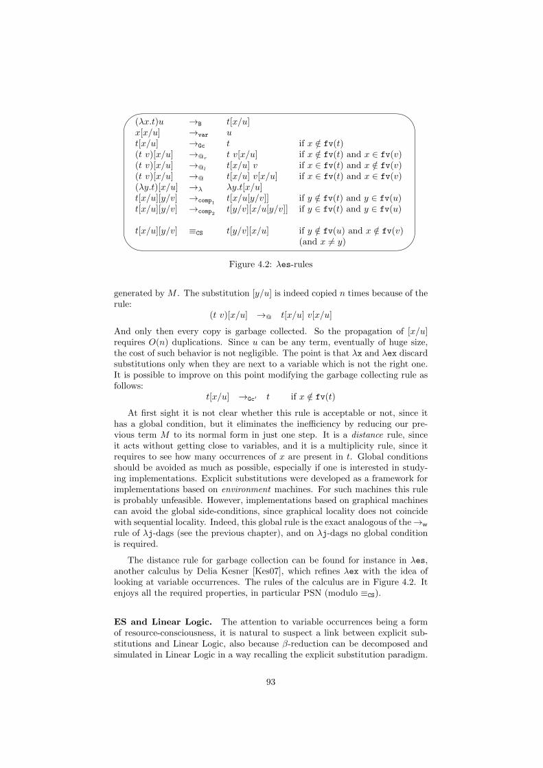
(λx.t)u →B t[x/u]x[x/u] →var ut[x/u] →Gc t if x /∈ fv(t)(t v)[x/u] →@r t v[x/u] if x /∈ fv(t) and x ∈ fv(v)(t v)[x/u] →@l t[x/u] v if x ∈ fv(t) and x /∈ fv(v)(t v)[x/u] →@ t[x/u] v[x/u] if x ∈ fv(t) and x ∈ fv(v)(λy.t)[x/u] →λ λy.t[x/u]t[x/u][y/v] →comp1

t[x/u[y/v]] if y /∈ fv(t) and y ∈ fv(u)t[x/u][y/v] →comp2

t[y/v][x/u[y/v]] if y ∈ fv(t) and y ∈ fv(u)

t[x/u][y/v] ≡CS t[y/v][x/u] if y /∈ fv(u) and x /∈ fv(v)(and x 6= y)

Figure 4.2: λes-rules

generated by M . The substitution [y/u] is indeed copied n times because of therule:

(t v)[x/u] →@ t[x/u] v[x/u]

And only then every copy is garbage collected. So the propagation of [x/u]requires O(n) duplications. Since u can be any term, eventually of huge size,the cost of such behavior is not negligible. The point is that λx and λex discardsubstitutions only when they are next to a variable which is not the right one.It is possible to improve on this point modifying the garbage collecting rule asfollows:

t[x/u] →Gc′ t if x /∈ fv(t)

At first sight it is not clear whether this rule is acceptable or not, since ithas a global condition, but it eliminates the inefficiency by reducing our pre-vious term M to its normal form in just one step. It is a distance rule, sinceit acts without getting close to variables, and it is a multiplicity rule, since itrequires to see how many occurrences of x are present in t. Global conditionsshould be avoided as much as possible, especially if one is interested in study-ing implementations. Explicit substitutions were developed as a framework forimplementations based on environment machines. For such machines this ruleis probably unfeasible. However, implementations based on graphical machinescan avoid the global side-conditions, since graphical locality does not coincidewith sequential locality. Indeed, this global rule is the exact analogous of the→w

rule of λj-dags (see the previous chapter), and on λj-dags no global conditionis required.

The distance rule for garbage collection can be found for instance in λes,another calculus by Delia Kesner [Kes07], which refines λex with the idea oflooking at variable occurrences. The rules of the calculus are in Figure 4.2. Itenjoys all the required properties, in particular PSN (modulo ≡CS).

ES and Linear Logic. The attention to variable occurrences being a formof resource-consciousness, it is natural to suspect a link between explicit sub-stitutions and Linear Logic, also because β-reduction can be decomposed andsimulated in Linear Logic in a way recalling the explicit substitution paradigm.

93

The link has been formalized by Kesner and co-authors [CKP03, KL07, KR09].First a translation of a typed ES-calculus into Linear Logic Proof-Nets [CKP03]has been used as a method to infer PSN for an ES-calculus from the strongnormalization of Proof-Nets (the calculus in that paper is not λes, which how-ever maps on Proof-Nets too). Then Kesner and Lengrand introduce in [KL07]a calculus reflecting the syntax of Proof-Nets, having not only explicit substi-tutions but also explicit contractions and weakenings. Last, in [KR09] Kesnerand Renaud show that these three explicit constructs can be independently andmodularly added to the λ-calculus, getting a prismoid of explicit operators (inanalogy to the famous λ-cube).

All these works have exploited ideas, results and syntax from Proof-Nets,also leading to modifications of the Proof-Nets syntax in order to smoothly ac-commodate the representation of explicit substitutions [CG99]. However, noneof these works has made the further step done here: to endow the term languagewith the operational semantics, and not just the syntax, of the graphical formal-ism. In general the calculus can be translated and simulated by the graphicalformalism, but the relation between terms and nets is not a strong bisimulation.

Distance and multiplicities. This further step, technically achieved in sec-tion 3.6 (page 77) through the sequentialization theorem of λj-dags, gives whatwe have called the structural λ-calculus, noted λj, which is a new formalismre-shaping the paradigm of explicit substitutions. From a term language per-spective it can be seen as bringing to the extreme consequence the at a distancetrick for the optimized garbage collection rule. Once we admit to garbage collectat a distance it is natural to change the var rule:

x[x/u] →var u

As follows:t[x/u] →var′ tx/u if |t|x = 1

Where |t|x denotes the number of free occurrences of x in t. The use of an im-plicit substitution for describing the rule is suspicious, but it is justified by whathappens graphically, where no meta-rule is required: the implicit substitutionis the only way we have to describe the graphical rule.

The peculiarity of these two rules at a distance,→var′ and→Gc′ , is that theydo not look to the constructor at the left of the explicit substitution [x/u], theydo not act following a proximity principle. Being extreme and coherent withthis new ideology it is natural to have a distance rule for the case |t|x > 1. Butwhat should we do in such a case? Clearly a duplication:

t[x/u] →c t[y]x [x/u][y/u] if |t|x ≥ 2

Where the notation t[y]x means that a non-empty proper subset of the occur-rences of x in t has been renamed y (for a formal definition see page 78). This setof rules, which can be seen to correspond the weakening/dereliction/contractionrule of Proof-Nets cut-elimination (see chapter 5), is enough to fully reduce sub-stitutions, getting even full-composition, without any need of propagations. Forinstance:

94

(x x)[z/z′][x/y] →c (x1 x2)[z/z′][x1/y][x2/y] →var′

(y x2)[z/z′][x2/y] →var′

(y y)[z/z′] →Gc′ y y

It is a very compact rewriting system. We get rid of the inefficient rule:

(t v)[x/u] →@ t[x/u] v[x/u]

Without having all the rules of λes. And full composition holds without usinga congruence nor a composition rule. In particular, no rewriting modulo isrequired.

The main objection to such set of rules is that they require global side con-ditions. This is certainly true, but it does not mean that they are unfeasible. InProof-Nets or λj-dags they can be performed without any global side-condition.Graphical formalisms represent locally the set of occurrences of the same vari-able, while sequential languages, using names, spread them all over the term.Concerning the original motivation for ES-calculi, λj can be understood as atool to formally study graphical implementations.

The structural λ-calculus is an algebrization of the graphical operationalsemantics, and the peculiar form of its rules comes form the fact that graphicaland sequential locality do not match. This is one of the reasons why it isinteresting to develop graphical syntaxes: they give new deep intuitions on thenature of computation.

A further example of this fact is that the B-rule creating substitutions getsdeformed when we try to faithfully reflect the corresponding graphical rule. Aswe have proved it becomes:

(λx.t)L u →dB t[x/u]L

Where L is a list of explicit substitutions. The intuitions is that the graphicalconstructors corresponding to the λ and the application are next to each otherin the graphical representation of (λx.t)L u, so that they form a local graphicalredex. This rule, surprisingly, is the key for many interesting properties of thestructural λ-calculus.

For very different motives it notably appears in weak ES calculi [LM99] too.Weak ES calculi forbid or constrain reduction under λ-abstractions, in particularsubstitutions cannot propagate through λs. Consequently there are potentialβ-redexes blocked by substitutions which will never be reduced. The dB rulehelps to avoid this problem.

The structural λ-calculus. In this chapter we show that λj enjoys full-composition, confluence and PSN, so proving the sanity properties of ES-calculi.But we shall go further showing that it is a concise and expressive tool to studythe rewriting theory of λ-calculus, revisiting the way redexes are created in theλ-calculus.

95

In chapter 5 we will show that λj is more than simply inspired from LinearLogic: λj is bond to the standard Proof-Nets representation of λ-calculus by thesame strong kind of relation which connects λj and λj-dags. This is a strongjustification for λj. Through λj we shall also revisit Regnier’s σ-equivalenceand linear head reduction.

In chapter 6 we will consider extensions of λj with commutative rules, i.e.,propagation of ES, in particular composition and decomposition of ES.

Despite calculi with explicit substitutions are the obvious reference for λj,the mechanism at work should in our opinion be considered a different, moreprimitive paradigm. For this reason in [AK10] we have called the construct[x/u] a jump rather than an explicit substitution, which is a suggestive name ex-pressing the idea that in λj [x/u] acts at a distance. In the wider context of thisthesis this is slightly improper, since it superposes with the already presentedgraphical concept of jump, which is only a part of the graphical constructionrepresenting [x/u]. However, we shall occasionally use this term rather than theheavier explicit substitution.

Let us conclude saying that of course some calculi using either distanceor multiplicities already exist, but without combining the two: only togetherthose concepts unleash their full expressive power. Indeed, [dB87, Ned92]use distance rules to refine β-reduction, but add ES to the syntax withoutdistinguishing between dereliction and contraction. Milner defines a λ-calculuswith ES inspired by another graphical formalism, Bigraphs [Mil07] (see section3.6.1), where ES also act at a distance. Again, he neither distinguishes betweendereliction and contraction, nor does his β-rule exploit distance. The same goesfor [SP94, Con06].

For lack of distance or sensibility to multiplicity none of these calculi canexpress the revisitation of redex creations, or of σ-equivalence, we shall showin this and the next chapter. Last, none of these formalisms enjoys a perfectmatch with a graphical formalism as it is the case for λj.

4.2 λj: basic properties

We recall the definition of λj.

Definition 4.1 (structural λ-calculus). The structural λ-calculus λj is givenby the language of λj-terms, generated by the following grammar:

t ::= x | λx.t | t t | t[x/t]

And by the following root rewriting rules:

(dB) (λx.t)L u 7→dB t[x/u]L(w) t[x/u] 7→w t if |t|x = 0(d) t[x/u] 7→d tx/u if |t|x = 1(c) t[x/u] 7→c t[y]x [x/u][y/u] if |t|x > 1

Where |t|x denotes the multiplicity of the variable x in the term t,which is the number of occurrences of x in t (formal definition at page 3.42),

96

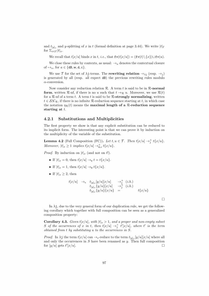
and t[y]x and y-splitting of x in t (formal definition at page 3.44). We write |t|Γfor Σx∈Γ|t|x.

We recall that t[x/u] binds x in t, i.e., that fv(t[x/u]) = (fv(t)\x)∪fv(u).

We close these rules by contexts, as usual: →a denotes the contextual closureof 7→a, for a ∈ dB,w, d, c.

We use T for the set of λj-terms. The rewriting relation →λj (resp. →j)is generated by all (resp. all expect dB) the previous rewriting rules moduloα-conversion.

Now consider any reduction relation R. A term t is said to be in R-normalform, written R-nf, if there is no u such that t →R u. Moreover, we use R(t)for a R-nf of a term t. A term t is said to be R-strongly normalizing, writtent ∈ SNR, if there is no infinite R-reduction sequence starting at t, in which casethe notation ηR(t) means the maximal length of a R-reduction sequencestarting at t.

4.2.1 Substitutions and Multiplicities

The first property we show is that any explicit substitution can be reduced toits implicit form. The interesting point is that we can prove it by induction onthe multiplicity of the variable of the substitution.

Lemma 4.2 (Full Composition (FC)). Let t, u ∈ T . Then t[x/u] →+j tx/u.

Moreover, |t|x ≥ 1 implies t[x/u]→+d,c tx/u.

Proof. By induction on |t|x (and not on t!).

• If |t|x = 0, then t[x/u]→w t = tx/u.

• If |t|x = 1, then t[x/u]→d tx/u.

• If |t|x ≥ 2, then

t[x/u] →c t[y]x [y/u][x/u] →+j (i.h.)

t[y]xy/u[x/u] →+j (i.h.)

t[y]xy/ux/u = tx/u

In λj, due to the very general form of our duplication rule, we get the follow-ing corollary which together with full composition can be seen as a generalizedcomposition property:

Corollary 4.3. Given t[x/u], with |t|x > 1, and a proper and non-empty subsetS of the occurrences of x in t, then t[x/u] →+

j t′[x/u], where t′ is the termobtained from t by substituting u to the occurrences in S.

Proof. In λj the term t[x/u] can→c-reduce to the term t[y]x [y/u][x/u] where alland only the occurrences in S have been renamed as y. Then full compositionfor [y/u] gets t′[x/u].

97

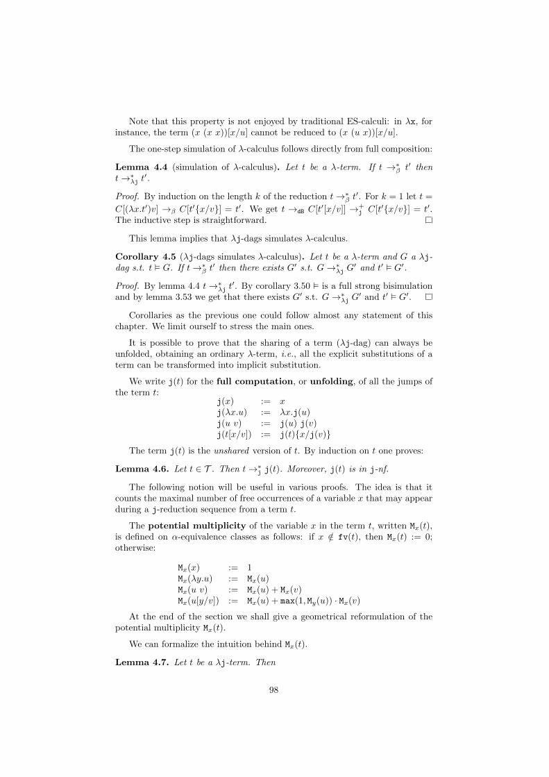
Note that this property is not enjoyed by traditional ES-calculi: in λx, forinstance, the term (x (x x))[x/u] cannot be reduced to (x (u x))[x/u].

The one-step simulation of λ-calculus follows directly from full composition:

Lemma 4.4 (simulation of λ-calculus). Let t be a λ-term. If t →∗β t′ thent→∗λj t′.

Proof. By induction on the length k of the reduction t→∗β t′. For k = 1 let t =

C[(λx.t′)v] →β C[t′x/v] = t′. We get t →dB C[t′[x/v]] →+j C[t′x/v] = t′.

The inductive step is straightforward.

This lemma implies that λj-dags simulates λ-calculus.

Corollary 4.5 (λj-dags simulates λ-calculus). Let t be a λ-term and G a λj-dag s.t. t G. If t→∗β t′ then there exists G′ s.t. G→∗λj G′ and t′ G′.

Proof. By lemma 4.4 t→∗λj t′. By corollary 3.50 is a full strong bisimulationand by lemma 3.53 we get that there exists G′ s.t. G→∗λj G′ and t′ G′.

Corollaries as the previous one could follow almost any statement of thischapter. We limit ourself to stress the main ones.

It is possible to prove that the sharing of a term (λj-dag) can always beunfolded, obtaining an ordinary λ-term, i.e., all the explicit substitutions of aterm can be transformed into implicit substitution.

We write j(t) for the full computation, or unfolding, of all the jumps ofthe term t:

j(x) := xj(λx.u) := λx.j(u)j(u v) := j(u) j(v)j(t[x/v]) := j(t)x/j(v)

The term j(t) is the unshared version of t. By induction on t one proves:

Lemma 4.6. Let t ∈ T . Then t→∗j j(t). Moreover, j(t) is in j-nf.

The following notion will be useful in various proofs. The idea is that itcounts the maximal number of free occurrences of a variable x that may appearduring a j-reduction sequence from a term t.

The potential multiplicity of the variable x in the term t, written Mx(t),is defined on α-equivalence classes as follows: if x /∈ fv(t), then Mx(t) := 0;otherwise:

Mx(x) := 1Mx(λy.u) := Mx(u)Mx(u v) := Mx(u) + Mx(v)Mx(u[y/v]) := Mx(u) + max(1, My(u)) · Mx(v)

At the end of the section we shall give a geometrical reformulation of thepotential multiplicity Mx(t).

We can formalize the intuition behind Mx(t).

Lemma 4.7. Let t be a λj-term. Then

98

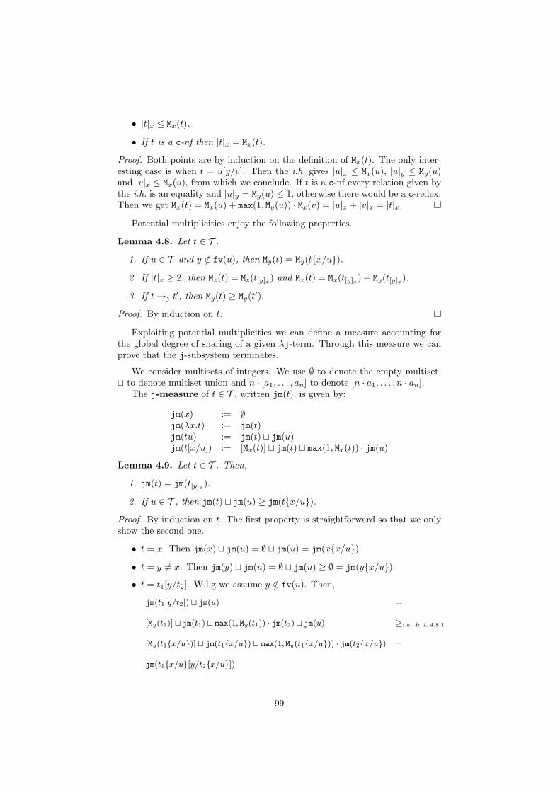
• |t|x ≤ Mx(t).

• If t is a c-nf then |t|x = Mx(t).

Proof. Both points are by induction on the definition of Mx(t). The only inter-esting case is when t = u[y/v]. Then the i.h. gives |u|x ≤ Mx(u), |u|y ≤ My(u)and |v|x ≤ Mx(u), from which we conclude. If t is a c-nf every relation given bythe i.h. is an equality and |u|y = My(u) ≤ 1, otherwise there would be a c-redex.Then we get Mx(t) = Mx(u) + max(1, My(u)) · Mx(v) = |u|x + |v|x = |t|x.

Potential multiplicities enjoy the following properties.

Lemma 4.8. Let t ∈ T .

1. If u ∈ T and y /∈ fv(u), then My(t) = My(tx/u).

2. If |t|x ≥ 2, then Mz(t) = Mz(t[y]x) and Mx(t) = Mx(t[y]x) + My(t[y]x).

3. If t→j t′, then My(t) ≥ My(t′).

Proof. By induction on t.

Exploiting potential multiplicities we can define a measure accounting forthe global degree of sharing of a given λj-term. Through this measure we canprove that the j-subsystem terminates.

We consider multisets of integers. We use ∅ to denote the empty multiset,t to denote multiset union and n · [a1, . . . , an] to denote [n · a1, . . . , n · an].

The j-measure of t ∈ T , written jm(t), is given by:

jm(x) := ∅jm(λx.t) := jm(t)jm(tu) := jm(t) t jm(u)jm(t[x/u]) := [Mx(t)] t jm(t) t max(1, Mx(t)) · jm(u)

Lemma 4.9. Let t ∈ T . Then,

1. jm(t) = jm(t[y]x).

2. If u ∈ T , then jm(t) t jm(u) ≥ jm(tx/u).

Proof. By induction on t. The first property is straightforward so that we onlyshow the second one.

• t = x. Then jm(x) t jm(u) = ∅ t jm(u) = jm(xx/u).

• t = y 6= x. Then jm(y) t jm(u) = ∅ t jm(u) ≥ ∅ = jm(yx/u).

• t = t1[y/t2]. W.l.g we assume y /∈ fv(u). Then,

jm(t1[y/t2]) t jm(u) =

[My(t1)] t jm(t1) t max(1, My(t1)) · jm(t2) t jm(u) ≥i.h. & L.4.8:1

[My(t1x/u)] t jm(t1x/u) t max(1, My(t1x/u)) · jm(t2x/u) =

jm(t1x/u[y/t2x/u])

99

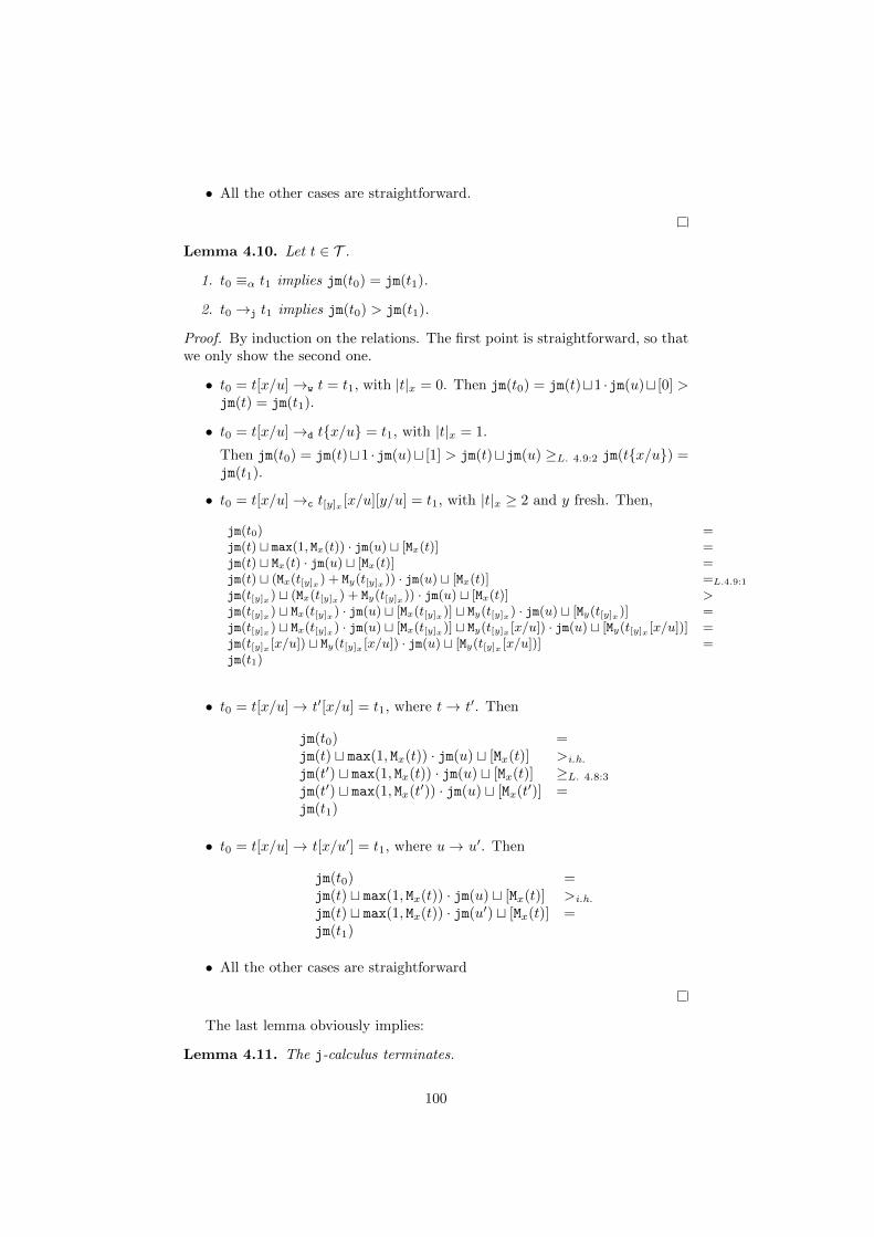
• All the other cases are straightforward.

Lemma 4.10. Let t ∈ T .

1. t0 ≡α t1 implies jm(t0) = jm(t1).

2. t0 →j t1 implies jm(t0) > jm(t1).

Proof. By induction on the relations. The first point is straightforward, so thatwe only show the second one.

• t0 = t[x/u]→w t = t1, with |t|x = 0. Then jm(t0) = jm(t)t1 ·jm(u)t [0] >jm(t) = jm(t1).

• t0 = t[x/u]→d tx/u = t1, with |t|x = 1.

Then jm(t0) = jm(t)t1 ·jm(u)t [1] > jm(t)tjm(u) ≥L. 4.9:2 jm(tx/u) =jm(t1).

• t0 = t[x/u]→c t[y]x [x/u][y/u] = t1, with |t|x ≥ 2 and y fresh. Then,

jm(t0) =jm(t) t max(1, Mx(t)) · jm(u) t [Mx(t)] =jm(t) t Mx(t) · jm(u) t [Mx(t)] =jm(t) t (Mx(t[y]x) + My(t[y]x)) · jm(u) t [Mx(t)] =L.4.9:1

jm(t[y]x) t (Mx(t[y]x) + My(t[y]x)) · jm(u) t [Mx(t)] >jm(t[y]x) t Mx(t[y]x) · jm(u) t [Mx(t[y]x)] t My(t[y]x) · jm(u) t [My(t[y]x)] =jm(t[y]x) t Mx(t[y]x) · jm(u) t [Mx(t[y]x)] t My(t[y]x [x/u]) · jm(u) t [My(t[y]x [x/u])] =jm(t[y]x [x/u]) t My(t[y]x [x/u]) · jm(u) t [My(t[y]x [x/u])] =jm(t1)

• t0 = t[x/u]→ t′[x/u] = t1, where t→ t′. Then

jm(t0) =jm(t) t max(1, Mx(t)) · jm(u) t [Mx(t)] >i.h.

jm(t′) t max(1, Mx(t)) · jm(u) t [Mx(t)] ≥L. 4.8:3

jm(t′) t max(1, Mx(t′)) · jm(u) t [Mx(t′)] =jm(t1)

• t0 = t[x/u]→ t[x/u′] = t1, where u→ u′. Then

jm(t0) =jm(t) t max(1, Mx(t)) · jm(u) t [Mx(t)] >i.h.

jm(t) t max(1, Mx(t)) · jm(u′) t [Mx(t)] =jm(t1)

• All the other cases are straightforward

The last lemma obviously implies:

Lemma 4.11. The j-calculus terminates.

100

Moreover:

Lemma 4.12. The j-nf of t ∈ T , written j(t), is unique.

Proof. One first shows local confluence and then Lemma 4.11 allows to applyNewman’s Lemma to conclude.

Both potential multiplicities and the j-measure can however be incrementedby dB-steps. Consider:

t = (λx.x x) y →dB (x x)[x/y] = t′

We get My(t) = 1, My(t′) = 2, jm(t) = ∅ and jm(t′) = [2].

We conclude the part on the elementary properties of λj by showing thepostponement of the erasing steps. We use →¬w for →dB,d,c. We need thefollowing lemma:

Lemma 4.13. Let t ∈ T . Then:

1. t→w→dB t′ implies t→dB→w t

′

2. t→w→d t′ implies t→d→w t

′

3. t→w→c t′ implies t→c→+

w t′

4. t→+w→¬w t′ implies t→¬w→+

w t′

Proof. Points 1-3 are by induction on the relations and case analysis. Point4 is by induction on the length k of →+

w . The case k = 1 is given by points1-3. If k > 1 then t →k

w→¬w t′ implies t →k−1w →¬w→+

w t′ and by i.h. we gett→¬w→+

w→+w t′.

Let us use τ : t→∗ t′ as a notation for a reduction sequence τ , the symbol ’;’for the concatenation of reduction sequences and |τ |¬w for the number of →¬wsteps in τ . Then we obtain:

Lemma 4.14 (w-postponement). Let t ∈ T . If τ : t →∗λj t′ then there exists areduction τ ′ : t→∗¬w→∗w t′ s.t. |τ |¬w = |τ ′|¬w.

Proof. By induction on k = |τ |¬w. Let k > 0. If τ : t→¬w u→∗λj t′ then simplyuse the i.h. on the sub-reduction ρ : u→∗λj t′. Otherwise τ = τw;→¬w ;ρ whereτw is the maximal prefix of τ made out of weakening steps only. By lemma 4.13.4we get that t→¬w→+

w ;ρ t and we conclude by applying the i.h. to →+w ;ρ.

4.2.2 Potential multiplicities, graphically

Potential multiplicities corresponds to the number of a certain type of paths inthe λj-dag of the term.

Definition 4.15 (skeletal path). A skeletal path in a λj-dag G is a path in G∗

s.t. it does not use any edge induced by a jump whose target is a non-weakeningvariable.

The next definition introduce a measure on the sharing nodes of G whichshall correspond exactly to the potential multiplicity of that variable in itscorresponding term.

101

Definition 4.16 (graphical multiplicity). Let G a λj-dag and x one of itssharing node. The graphical multiplicity GMx(G) of x in G is the numberof skeletal paths from the root r to x, if x is a free sharing node of G, and 0otherwise.

Lemma 4.17. Let G be a λj-dag. Then any non-weakening sharing node of Ghas at least a skeletal path from the root.

Proof. By induction on the number of links of G, acting on the root.

Lemma 4.18. Let t be a λj-term and G = t. Then GMx(G) = Mx(t) for everyfree variable x of t.

Proof. By induction on t. If t = x it is obvious. The application and abstractioncase follow immediately by the i.h. and the definition of the translation ·. Solet t = s[y/v]. By i.h. we get GMy(s) = My(s) and GMx(v) = Mx(v).By internal closure of G↓y = v any path to one of its free variables has to passthrough y. Since y is maximal in j(r) every exit of v is an exit of G = t and soevery skeletal path using edges of v has a suffix in v. Let τ be a skeletal pathfrom the root to x. Either τ is a skeletal path to y followed from a skeletal pathfrom y to x or it does not use any edge of v, and so it is a skeletal path of t 6↑y,too. So we get GMx(t) = GMx(t 6↑y) +A ·GMx(v), where A is the number of skeletalpaths from the root to y. But by sequentialization we get sy = t6↑y and sy ands have the same skeletal paths, so GMx(t 6↑y) +A · GMx(v) =i.h. Mx(s) +A · Mx(v).The path contributing to A are those of GMy(s) with the exception that if y isthe node of a weakening (which gives GMy(s) = 0) then in t there is a jump to it,which counts as a skeletal path, and so in such a case we rather get A = 1. Bylemma 4.17 in every other case we have My(u) ≥ 1 and so A = max(1, My(u)).

4.2.3 Confluence

Confluence of calculi with ES can be easily proved by using Tait and MartinLof’s technique (see for example the case of λes [Kes07]). This technique isbased on the definition of a simultaneous reduction relation Vλj which enjoysthe diamond property. It is completely standard so we give the statements ofthe lemmas and omit the proofs.

The simultaneous reduction relation Vλj is defined on terms in j-normal form as follows:

• xVλj x

• If tVλj t′, then λx.tVλj λx.t

′

• If tVλj t′ & uVλj u

′, then t uVλj t′ u′

• If tVλj t′ and uVλj u

′, then (λx.t) uVλj j(t′[x/u′])

A first lemma assures that Vλj can be simulated by →λj.

Lemma 4.19. If tVλj t′, then t→∗λj t′.

Proof. By induction on tVλj t′.

A second lemma assures that →λj can be projected through j(·) on Vλj.

102

Lemma 4.20. If t→λj t′, then j(t)Vλj j(t′).

Proof. By induction on t→λj t′.

The two lemmas combined essentially say that Vλj is confluent if and onlyif→∗λj is confluent. Then we show the diamond property forVλj, which impliesthat Vλj is confluent:

Lemma 4.21. The relation Vλj enjoys the diamond property.

Proof. By induction on Vλj and case analysis.

Then we conclude:

Theorem 4.22 (Confluence). For all t, u1, u2 ∈ T , if t→∗λj ui (i = 1, 2), then∃v s.t. ui →∗λj v (i = 1, 2).

Proof. Let t →∗λj ti for i = 1, 2. Lemma 4.20 gives j(t) V∗λj j(ti) for i = 1, 2.Lemma 4.21 implies Vλj is confluent so that ∃s such that j(ti) V∗λj s for i =1, 2. We can then close the diagram with ti →∗j j(ti)→∗λj s by Lemma 4.19.

Corollary 4.23. λj-dags are confluent.

Proof. The λj-calculus is confluent (theorem 4.22) and confluence is preservedby full strong bisimulations with the unicity property as in the statement oflemma 3.56 (page 85). Since the read-back of λj-dags is a full strong bisimula-tion with such property (theorem 3.49, page 80) we conclude.

Lemma 4.24. The structural λ-calculus is Church-Rosser modulo ≡CS.

Proof. By theorem 4.22, lemma 3.61 and the fact that ≡CS is an internal strongbisimulation of the structural λ-calculus which is an equivalence relation (lemma3.51, page 82).

Sometimes a stronger property than confluence is asked to ES-calculi, con-fluence in presence of meta-variables (which are used in the framework of higher-order unification [Hue76]). The idea is to switch to an enriched language with anew kind of variables of the form X∆, to be intended as a named context holeaccepting to be replaced by terms whose free variables are among ∆. In pres-ence of meta-variables not all the substitutions can be computed. Consider forinstance Xy[y/z]: the substitution is blocked. However, in general it is enoughto add ≡CS to recover confluence. Since λj-dags are exactly a representation ofλj/CS, and the structural λ-calculus is Church-Rosser modulo ≡CS, we believethat confluence on meta-variables for λj/CS easily follows.

Consider the following example of critical pair of λes (rules in Figure 4.2,page 93):

((λx.X∆) z)[y/v] →@l ((λx.X∆)[y/v] z) →λ (λx.X∆[y/v]) z

↓B ↓B

X∆[x/z][y/v] X∆[y/v][x/z]

103

In presence of meta-variables this is the pair requiring ≡CS in order to beclosed. The problem is generated by the propagation→@l , which does not existin λj. It is natural to wonder if λj is confluent on meta-variables even without≡CS. The answer is no. Consider:

(Xz Y z)[z/z′]

It reduces both to (Xz1 Y z2)[z1/z′][z2/z

′] and (Xz1 Y z2)[z2/z′][z1/z

′],and ≡CS is necessary in order to restore confluence.

4.3 Preservation of β-Strong Normalization

A reduction system R for a language containing the λ-calculus is said to en-joy the PSN property iff every λ-term which is β-terminating is also R-terminating (on the same normal form).

Usually the PSN property, when it holds, has an involved non-trivial proof.The main reasons of its complexity are:

• Usually the framework where a termination result is studied is a calculuswhere every term terminates. But in the λ-calculus there are divergingterms. In fact, the PSN is a conditional termination property: if a λ-termt terminates when evaluated with β-reduction then it terminates whenevaluated with the ES-reduction system.

• The setting is untyped, so many techniques for termination exploiting thetype of the term, notably the reducibility candidates technique, cannot beapplied.

• The reductions of the ES-system can be easily projected on the λ-calculusthrough the map j(·) which transforms every explicit substitution in animplicit substitution, but this map does not preserve divergence. Forinstance, consider t = x[y/s] where s is a diverging term. Then j(t) = xwhich is a normal form while t is not strongly normalizing.

We shall see that there is another reason why such proofs are usually com-plex: ES-calculi propagates substitutions through the term structure, which isthe language analogous of commutative cut-elimination steps in sequent calcu-lus. Removing the commutative cases, indeed, the proof becomes incrediblyconcise, although still non-trivial.

Before the formal development we want to stress the power of a PSN re-sult. Its important corollaries are strong normalization results in all main typedframeworks. Explicit substitutions are typable with intersection, second-orderor simple types by extending the usual systems with the following cut rule:

∆ ` u : A ∆, x : A ` t : B

∆ ` t[x/u] : B

To reduce typability of terms with ES to typability of ordinary λ-terms onedefines the B-expansion of a λj term:

104

Bexp(x) := xBexp(λx.u) := λx.Bexp(u)Bexp(u v) := Bexp(u) Bexp(v)Bexp(u[x/v]) := (λx.Bexp(u)) Bexp(v)

An induction on the definition proves that Bexp(t) is an ordinary λ-term andthat Bexp(t) is typable in the intersection/second-order/simple ordinary typesystem if and only if t is typable in the corresponding ES-typing system. Thenwe conclude since Bexp(t) is SN λ by the standard results on λ-calculus, soBexp(t) is SN λj by PSN and Bexp(t) →∗dB t, which gives t ∈ SN λj (the samereasoning can be carried out in any ES-calculus enjoying PSN).

The elegant proof technique we are going to use has been developed by DeliaKesner and it uses an inductive characterization of the strongly normalizing λ-terms, that can be found for instance in [vR96] (page 47):

x ∈ V M1, . . . ,Mk ∈ SNλvar

xM1 . . .Mk ∈ SNλ

x ∈ V M ∈ SNλλ

λx.M ∈ SNλ

Mx/NN1 . . . Nk ∈ SNλ N ∈ SNλ@

(λx.M)NN1 . . . Nk ∈ SNλ

The technique reduces PSN to the IE property, which relates terminationof Implicit substitution to termination of Explicit substitution, and it is anabstract technique not depending on the particular form of the λj-calculus.

Let t1n denotes t1 . . . tn and R be a reduction system on the λj-language. R

is said to enjoy the IE property iff for n ≥ 0 and for all t, u, v1n ∈ λ-terms:

u ∈ SNR & tx/uv1n ∈ SNR imply t[x/u]v1

n ∈ SNR

Of course one generally considers a system R which can simulate the λ-calculus, otherwise everything is trivialized and uninteresting.

Theorem 4.25 (IE implies PSN). Let R be a calculus verifying the IE-propertyand the following facts:

(F0) If t1n ∈ λ-terms in SNR, then x t

1n ∈ SNR.

(F1) If u ∈ λ-term in SNR, then λx.u ∈ SNR.

(F2) The only R-reducts of a λ-term (λx.u) v t1n are u[x/v] t

1n as well as

the ones coming from internal reduction on u, v, t1, . . . , tn.

Then, R enjoys PSN.

Proof. We show that t ∈ SN β implies t ∈ SNR by induction on the inductivecharacterization of t ∈ SN β .

• If t = x t1n with ti ∈ SN β , then ti ∈ SNR by the i.h. and thus x t

1n ∈ SNR

by fact F0.

105

• If t = λx.u with u ∈ SN β , then u ∈ SNR by the i.h. and thus λx.u ∈SNR by fact F1.

• If t = (λx.u) v t1n, with ux/v t1n ∈ SN β and v ∈ SN β , then both terms

are in SNR by the i.h. IE gives U = u[x/v] t1n ∈ SNR, so in particular

u, v, t1 . . . , tn ∈ SNR.We show t ∈ SNR by induction on ηR(u) + ηR(v) + Σi ηR(ti). For that,it is sufficient to show that every R-reduct of t is in SNR.Now, if t →R t′ is an internal reduction, then apply the i.h. Otherwise,

fact F2 gives t→R u[x/v] t1n = U which is in SNR.

Since λj clearly satisfies the three requirements of the last theorem, in orderto get PSN for λj we only need to prove that it enjoys the IE property.

Theorem 4.26 (IE for λj). λj enjoys the IE property.

We prove the theorem by induction on a measure and show that any reductof M = t[x/u] v1

n has a smaller measure than M . But for the inductive stepto work (in particular in the case of a duplication) we need a version of IEgeneralized to possibly many substitution.

Notation: If m ≥ 1 we write [xi/ui]1m for [x1/u1] . . . [xm/um]. To improve

readability we shall also use [xi/ui]1m = [·]1m. Similarly for implicit substitutions.

Theorem 4.27 (Generalized IE for λj). For all λj-terms t, u1m (m ≥ 1), v1

n (n ≥0), if u1

m ∈ SN λj & txi/ui1mv1n ∈ SN λj, then t[xi/ui]

1mv

1n ∈ SN λj, where

xi 6= xj for i, j = 1 . . .m and xi /∈ fv(uj) for i, j = 1 . . .m.

The IE property then holds by taking m = 1. We recall that ηλj(t) is anotation for the maximal length of a λj-reduction sequence starting at t, andwe extend such notation to vectors of terms as follows: ηλj(u

1m) =

∑mi=1 ηλj(ui).

Proof. Suppose u1m ∈ SN λj & txi/ui1m v1

n ∈ SN λj. We show T = t[xi/ui]1m v1

n ∈SN λj by induction on

〈ηλj(txi/ui1m v1n), ox1

m(t), ηλj(u

1m)〉

where oxi(t) = 3|t|xi and ox1m

(t) = Σi∈moxi(t).To show T ∈ SN λj it is sufficient to show that every λj-reduct of T is in

SN λj.

• T →λj t[·]1j−1[xj/u′j ][·]j+1

m v1n = T ′ with uj →λj u

′j . Then we get:

– ηλj(t·1j−1xj/u′j·j+1m v1

n) ≤ ηλj(t·1m v1n),

– ox1m

(t) does not change, and

– ηλj(u1j−1u

′juj+1m ) < ηλj(u

1m).

We conclude by the i.h., since u1j−1u

′juj+1m ∈ SN λj and our hypothesis

txi/ui1mv1n ∈ SN λj is equal or reduces to t·1j−1xj/u′j·j+1

m v1n ∈

SN λj (depending on |t|xj ).

106

• T →λj t′[·]1m v1

n = T ′ with t→λj t′. Then we have that

ηλj(t′·1m v1

n) < ηλj(t·1m v1n)

We conclude by the i.h. since t′·1m v1n ∈ SN λj.

• T →λj t[·]1m v1 . . . v′i . . . vn = T ′ with vi →λj v

′i. Then we have that

ηλj(t·1m v1 . . . v′i . . . vn) < ηλj(t·1m v1

n)

We conclude by the i.h. since t·1m v1 . . . v′i . . . vn ∈ SN λj.

• T →w t[·]1j−1[·]j+1m v1

n, with |t|xj = 0. Then we have that

ηλj(t·1j−1·j+1m v1

n) = ηλj(t·1m v1n)

But o (t) decreases since ox1j−1x

j+1m

(t) < ox1m

(t). We conclude by the i.h.

since t·1j−1·j+1m v1

n = t·1m v1n ∈ SN λj by hypothesis.

• T →d t[·]1j−1xj/uj[·]j+1m v1

n with |t|xj = 1. Then we get

ηλj(t·1j−1xj/uj·j+1m v1

n) = ηλj(t·1m v1n)

Also, the jumps are independent, so that x1j−1x

j+1m ∩ fv(uj) = ∅ implies

ox1j−1x

j+1m

(txj/uj) < ox1m

(t).

We conclude since t·1j−1xj/uj·j+1m v1

n = t·1m v1n ∈ SN λj by hy-

pothesis.

• T →c t[y]xj[·]1j−1[xj/uj ][y/uj ][·]j+1

m v1n with |t|xj ≥ 2 and y fresh. Then,

ηλj(t[y]xj·1j−1xj/ujy/uj·j+1

m v1n) = ηλj(t·1m v1

n)) and

ox1j−1xjyx

j+1m

(t[y]xj) < ox1

m(t). In order to apply the i.h. to t[y]xj

we need.

– u1j−1, uj , uj , u

j+1m ∈ SN λj. This holds by hypothesis.

– t[y]x1·1j−1xj/ujy/uj·j+1

m v1n ∈ SN λj. This holds since the

term is equal to t·1m v1n which is SN λj by hypothesis.

This is the case that forces the generalized sequence of substitutions:if we were proving the statement for t[x/u] v1

n using as hypothesis u ∈SN λj & tx/u v1

n ∈ SN λj then there would be no way to use the i.h. toget t[y]x [x/u][y/u] v1

n ∈ SN λj.

• T = (λx.t′)[·]1m v1v2n →dB t

′[x/v1][·]1m v2n = T ′. We have that

U = (λx.t′)·1m v1v2n ∈ SN λj

holds by hypothesis. Using full composition we obtain

U →dB t′·1m[x/v1] v2n

→+λj t′·1mx/v1 v2

n

= t′x/v1·1m v2n = U ′

Thus ηλj(U′) < ηλj(U). To conclude T ′ ∈ SN λj by the i.h. we then need

107

– v1, u1m ∈ SN λj. But u1

m ∈ SN λj holds by hypothesis and txi/ui1m v1n ∈

SN λj implies v1 ∈ SN λj.

– U ′ = t′x/v1·1m v2n ∈ SN λj which holds since ηλj(U

′) < ηλj(U).

We then get:

Corollary 4.28 (PSN for λj). λj enjoys the PSN property, namely: if t is aλ-term and t ∈ SN β, then t ∈ SN λj.

And we also get the following corollaries:

Corollary 4.29. The reduction →λj modulo CS enjoys the PSN property.

Proof. Follows from Corollaries 4.28 and 3.58 and the fact that ≡CS is an internalstrong bisimulation.

Corollary 4.30. λj-dags enjoy the PSN property.

Proof. Follows from Corollaries 4.28 and 3.54 and the fact that is a full strongbisimulation.

Let us point out that despite the IE technique is due to Delia Kesner alone,its application to λj has been developed in collaboration with the author. Evenif she would have certainly been able to develop it without our help, we areparticularly proud of having contributed to such concise and elegant result,which in our opinion is the pearl of the thesis.

The fact that one can essentially reduce PSN to the one-page proof of justone statement is extra-ordinary, in the literal sense that ordinary ES-calculi havemuch more complex proofs of PSN, of pages and pages, passing through manyintermediary lemmas. In our opinion this is the main evidence of the relevanceof λj despite there exist dozens of ES-calculi.

The reason behind such conciseness is the fact that none of the rules of λjpropagates substitutions. Indeed, in presence of propagations the term structureis affected, which forbids to use the i.h.. So one needs to further generalize theshape of the statement, but it is not clear how.

Imagine to extend λj with a rule as:

(t v)[x/u] →b t v[x/u] if x /∈ fv(t)

Call this system λj′. To prove T = t[xi/ui]1m v1

n ∈ SN λj′ assuming u1m ∈

SN λj′ and txi/ui1m v1n ∈ SN λj′ by showing that every of its reducts is in

SN λj′ , which is what we did for proving theorem 4.26, requires to consider thecase where t = s w and

T = (s w)[xi/ui]1m v1

n →b (s w[x1/u1])[xi/ui]2m v1

n

But now how should we use the inductive hypothesis to prove that(s w[x1/u1])[xi/ui]

2m v1

n ∈ SN λj′? It seems that it is impossible. Of course one

108

may try to change the statement, has we did to handle duplications, but we donot know how this should be done, either.

In chapter 6 we will prove PSN for λj enriched with propagation rules. Weshall use another technique, and the complexity of the proof will explode, infact the whole chapter will be devoted to such proof(s). Of course this does notmean that there is no easy proof of PSN for systems with propagations. But15 years after Mellies negative result no such proof of PSN has been found yet.Moreover, the rule we showed can be seen as the term analogous of the box-boxrule of Linear Logic Proof-Nets. And there too, despite the typed framework,normalization proofs are hard and long.

There is a clear logical intuition behind this problem: sequent calculus cut-elimination redexes can be divided in two classes, key cases and commutativecases (An example can be found in subsection 8.1, page 186). The key casesdiminish the logical complexity of a proof, and are the interesting ones, whilethe commutative cases, corresponding to propagations, are re-arrangements ofthe proof structure needed to put in evidence hidden key cases. Most sequentcalculus and explicit substitution systems have rules for both kinds of cases,requiring termination proofs to integrate a reasoning about logical complexityand a reasoning about the re-arrangements of the term structure. For instancethis can be seen in the so-called Gandy method for termination, usually usedfor Proof-nets with the commutative box-box rule [PT09, PdF10], where thelong proof is split in two main parts, one proving weak normalization witha logical argument and another using non logical arguments to derive strongnormalization from the weak one.

Graphical languages allow to define systems without commutative cases (de-spite there exist graphical systems with commutative cases), which can readback as distance rules on terms or sequents, as for λj. In absence of commuta-tive cases the reasoning simplifies because it does not need to take into accountthe term structure. Indeed, note that our proof of the IE property does notmake induction on the term structure but only on the length of reductions andmultiplicities. Multiplicities certainly are a property of the term, but they donot depend on the inductive structure, rather on the naming, which is a moreabstract component of a term. Consider for instance t and t′ = t[y]x where|t|x > 1: the two terms have exactly the same mute structure, that is, modulothe name of variables they have the same constructors arranged in the sameway. So one may have different multiplicities within the same term structure.Also the opposite is possible: there may be different terms with the same mul-tiplicities. The abstract and pleasant character of multiplicities is that theydescribe the leaves of the term syntax tree ignoring the actual content of thetree. In particular they do not depend on the specific set of constructors, as itis the case for propagations, and reasonings about multiplicities are modular.

So it seems natural that λj with propagations requires a much heavier ma-chinery than λj alone. Of course a concise technique for termination in presenceof commutative cuts would be extremely interesting. But to the best of ourknowledge such technique has still to be found.

109

4.4 Developments and All That

A λ-term t is either a normal form or it contains some redexes. However, ifone reduces all the redexes in t it is not the case that the obtained term t′

is normal: redexes can be created dynamically, along a reduction. The richrewriting theory of λ-calculus stems from this fact.

Consider Ω = (λx.(x) x) λy.(y) y. It has only one redex and nonetheless itdiverges. Indeed,

Ω→ (λy.(y) y) λy.(y) y = t′

Where the redex in t′ has been created, since its ancestor application x x wasnot a redex in t.

There are two interesting facts about this phenomenon of creation. The firstis that reductions contracting only the redexes in the starting term t and theirresiduals have finite length, for no matter which term t. For instance, Ω has onlyone reduction of this kind, the one of length one that we showed. This meansthat divergence is intimately connected to creation of redexes. Remarkably,every maximal such reduction starting on t ends on the same term. This is thecontent of the finite developments theorem. Let us fix some terminology.

A reduction sequence starting at t is a development [Hin78] if only residualsof redexes of t are contracted. A maximal development, i.e., a developmentreducing all the residuals of redexes in t, is called a full development. Thestandard result is:

Theorem 4.31 (Finite developments). Any development of a λ-term t termi-nates and all full developments end on the same term.

There are many proofs of this theorem, like [Hin78, vR96]. Interestingly,the result of all full developments can be described easily by induction on thestructure of the term, through the following definition:

x := x((λx.t) u) := tx/u(λx.t) := λx.t

(t u) := t u if t 6= λ

Note that t 6= λ implies t 6= λ.

In λj, but also in other ES-calculi, it is possible to give an operationalcharacterization of t. Let B be the rewriting rule

(λx.t) u→B t[x/u]

Which is the restriction of our dB-rule to a proximity action, i.e., without anysubstitution between the abstraction and its argument. This relation is triviallycomplete, that is, confluent and strongly normalizing, so that we use B(t) forthe (unique) B-nf of the term t. We get:

Proposition 4.32. Let t ∈ λ-term. Then t = j(B(t)).

Proof. By induction on t.

• Case t = x. Then x = x = j(B(x)).

110

• Case t = λx.u. Then (λx.u) = λx.u =i.h. λx.j(B(u)).

• Case t = u v, where u 6= λ. We then have (u v) = u v =i.h.

j(B(u)) j(B(v)) =u6=λ j(B(u v)).

• Case t = (λx.u) v. We have t = ux/v =i.h. j(B(u))x/j(B(v)) =j(B(u)[x/B(v)]) = j(B((λx.u) v)).

The second interesting fact is that in λ-calculus the ways redexes are createdcan be classified in three types, according to Levy [Lev78]:

Type 1: ((λx.λy.t) u) v →β (λy.tx/u) v.

Type 2: ((λx.x) λy.t) u→β (λy.t) u.

Type 3: (λx.C[x v]) (λy.u)→β Cx/λy.u[(λy.u) (vx/λy.u)]

Let’s have a close look to them, through the lens of λj. In the left termM = ((λx.λy.t) u) v of the the first type the abstraction on y cannot interactwith v. The reduction of the β-redex (λx.λy.t) u creates the redex betweenλy and v. One important fact is that besides the creation mechanism the tworedexes are independent, in a strong sense. This can be easily seen in λj, whichis a very flexible tool to dissect β-reduction. Indeed, let us show what happensif we start the reductions of both redexes without completing them:

M →dB (λy.t)[x/u] v →dB t[x/u][y/v]

Modulo →dB steps, which are linear reductions, the two redexes are in par-allel: in fact t[x/u][y/v] ≡CS t[y/v][x/u], since clearly x /∈ fv(v) and y /∈ fv(u).Let us recall that ≡CS is exactly the quotient induced on λj-terms by the trans-lation on λj-dags, i.e., the two terms are mapped on the same λj-dag, wherethey are in parallel. This is a nice way to express the parallelism of the tworedexes.

One of the two axioms of Regnier’s σ-equivalence, notion which will be in-troduced and discussed in Section 5.2 (page 137), can be seen as a way to re-organize the constructors of a λ-term t so that the hidden redex in ((λx.λy.t) u) vbecomes visible: indeed M = ((λx.λy.t) u) v ∼σR1 (λx.((λy.t) v)) u = N holds,and in N the two redexes are indeed in parallel.

Now consider the term M = ((λx.x) λy.t) u causing the second type ofcreation. The firing of the identity redex (λx.x) λy.t → λy.t creates the redex(λy.t) u. Here the two redexes cannot be seen in parallel. In λj we get that

((λx.x) λy.t) u→dB x[x/λy.t] u→d (λy.t) u (4.1)

Where we stress that both steps are linear and no use of distance is required.

A development can be extended to also reduce created redexes of type 1and 2. This more liberal notion, called L-development here, is usually knownas superdevelopment [KvOvR93]. Maximal L-developments are called full L-developments. It is possible to generalize to L-developments the finite devel-opment theorem.

111

Theorem 4.33 (Finite L-development). Any L-developmentof a λ-term t ter-minates and all full developments end on the same term.

The result of a full L-development of a λ-term is unique and admits thefollowing inductive definition [KvOvR93]:

x := x(t u) := t u if t 6= λ(λx.t) := λx.t

(t u) := t1x/u if t = λx.t1

Note that t 6= λ implies t 6= λ. The difference between t and t is in thelast clause of the definition.

In λj there is an operational characterization of t similar to that of t

previously given. This will be shown in the following subsection. Let us continuewith our analysis of creations.

The firsts two types of creation are obtained by reducing the functional partof a non-redex application whose result gives an abstraction and so creates aredex. It is usually said the the redexes are created upwards, i.e., with respectto an application closer to the root than the reduced redex:

The third type of creations is quite different, and it is malicious, since itleads to divergence, even if taken alone: the creation of Ω is of type 3. Thegeneral initial term M = (λx.C[x v]) (λy.u) substitutes (λy.u) to x in C[x v]creating the redex (λy.u) (vx/λy.u), and eventually many others in vx/λy.uand Cx/λy.u[·]. In this case the application becomes a redex because of asubstitution originating from above, so it is often said that the redex has beencreated downwards. In the first type of creations the two redexes are in parallel,and in the second type the argument of the first redex becomes the functionof the second. Here something dangerous can happen: the argument of thefirst redex can become at the same time the function and the argument of thecreated redex(es), which happens for instance when v = x, as in Ω.

The addition of the third type to L-developments gets full β-reduction, soapparently there is no way of going further. However, in λj we can naturallyextend the characterization of L-developments to a stronger complete reduction,that we call XL-developments. The idea is to isolate the linear creations ofthe third type, which are of a benign nature. Consider the prototype M =(λx.C[x v]) (λy.u) of the third type. In λj we get:

M = (λx.C[x v]) (λy.u)→dB C[x v][x/λy.u]

Now there are two cases: either C[·] or v contain occurrences of x, and thenwe have to duplicate [x/λy.u], or they do not and we can continue withoutduplicating:

C[x v][x/λy.u]→d C[(λy.u) v]

The idea is that the second case of third type creations is innocent, theintuition coming from the fact that Ω creates redexes using duplication. In λjit is possible to separate the two creations, and we can prove that our intuitionis correct: L-developments can be extended to XL-developments, catching linearcreation of the third type, which are confluent and terminating.

112

Then it is possible to refine the picture of creation mechanisms in the fol-lowing way:

Type 1: ((λx.λy.t) u) v →β (λy.tx/u) v.

Type 2: (λx.x) (λy.t) u→β (λy.t) u.

Linear Type 3: M = (λx.C[x v]) (λy.u) and |C[v]|x = 0, then M →β

C[(λy.u) v].

Non-Linear Type 3: M = (λx.C[x v]) (λy.u) and |C[v]|x > 0, thenM →β Cx/λy.u[(λy.u) (vx/λy.u)].

XL-developments catch type 1, 2 and the linear type 3. In order to define XL-developments is then crucial to have rewriting rules depending on multiplicities.For instance Milner’s calculus λm (see subsection 3.6.1, page 82) cannot describeXL-developments.

The following table summarizes the behavior of each computational notionstudied in this section on the λ-term u0 = (I I) ((λz.z y) I), where I = λx.x.

Full development of u0 = I (I y)Full L-development of u0 = I yFull XL-development of u0 = y

(4.2)

4.4.1 Catching L-developments

Let us recover t by means of our language λj. As for developments we shalluse a pair of subsystems. The key to operationally describe the first type ofcreation is the distance dB-rule, whose (unique) nf will be noted dB(t). In ourcharacterization of the result of a full development t we constrained dB to aproximity, distance-free, version B. For catching the first type of creations weonly have to remove the constraint. Replacing our definition of developmentj(B(t)) with j(dB(t)) gives:

dB(((λx.λy.t) u) v) = dB((λy.t)[x/u] v) =(∗)dB(t[y/v][x/u]) = dB(t)[y/dB(v)][x/dB(u)]

Where the step (*) is given by the removal of the constraint on the distance.Then, computing the explicit substitution, we get:

j(dB(((λx.λy.t)u)v)) = j(dB(t)[y/dB(v)][x/dB(u)]) =j(dB(t))x/j(dB(u))y/j(dB(v))

And we are done.

Let us call a full 1-development of a term t a reduction contracting all theredexes in the initial term plus those obtained dynamically by creation of type1 only. Interestingly, there is no characterization by induction on t of the resultof a full 1-development, or at least we were unable to find it in the literature.We just showed that this can be done in λj in a natural way.

Now, to specify L-developments within our language we also need to capturethe second type of creation. We showed in (4.1), page 111, that those creations

113

need to include into the first subsystem the dereliction rule. We would thereforeneed to use dB ∪ d instead of dB, but our (distance) d-rule turns out to be toopowerful since created redexes of type 3 would also be captured as shown by:

(λx.x z) (λy.u) →dB (x z)[x/λy.u] →d (λy.u) z →dB u[y/z]→ ...

Thus, the reduction d has to be restricted to act on variables only: thereduction →md (for minimal dereliction) is the context closure of the rule:

x[x/u]→ u

That is, d where we have removed the distance. The idea is that t can beobtained by first taking the normal form with respect to dB ∪ md and then byeliminating substitutions through j(·), generalizing the way we catched t.

Curiously, we have to enlarge a bit the first subsystem, otherwise the char-acterization does not hold. We have to add →w since weakening substitutionmay be a dummy context for x blocking →md, i.e., we can end up with a termx[y/y′][x/λz.t] u where we should substitute x and keep reducing the new redex(λz.t) u but this is not allowed because [y/y′] blocks →md. Consider the terms = ((λx.((λy.x) t)) λz.z) z′ and let us β-reduce the two redexes in s:

s = ((λx.((λy.x) y′)) λz.z) z′ →β ((λx.x) λz.z) z′ →β (λz.z) z′

Where we have underlined the redex reduced at each step. The redex(λz.z) z′ comes from a creation of the second type, and so an L-developmentwould reduce it, getting s = z′. But in λj:

s = ((λx.((λy.x) y′)) λz.z) z′ →dB

(λx.(x[y/y′]) λz.z) z′ →dB x[y/y′][x/λz.z] z′

And we have reached the →dB∪md normal form. Then we compute substitu-tions getting the term j(x[y/t][x/λz.z] z′) = (λz.z) z′, which is not s = z′.If we allow →d to reduce through substitution contexts we get a too powerfulreduction, reducing more than L-developments. The right thing to do is to add→w to the first subsystem. We then define A be the relation dB ∪ md ∪ w.

Lemma 4.34. The reduction relation →A is complete.

Proof. Termination of A is straightforward. Confluence follows from local con-fluence (straightforward by case-analysis) and Newman’s Lemma.

We want to prove

Proposition 4.35. Let M be a λ-term. Then M = j(A(M)).

The proof is by induction on M . Three cases out of four are straightforward,just apply the i.h.:

• Case M = x. Then x = x = j(A(x)).

• Case M = λx.t. Then (λx.t) = λx.t =i.h. λx.j(A(t)) = j(A(M)).

114

• Case M = t u, where t 6= λ. By the i.h. we get t = j(A(t)), hencej(A(t)) 6= λ and A(t) 6= λ. We then have:

(t u) = t u =i.h.

j(A(t)) j(A(u)) =j(A(t) A(u)) = j(A(t u))

The difficult case is the one corresponding to the following clause of thedefinition of t:

(t u) := t1x/u if t = λx.t1

Using the i.h. one gets t = λx.t1 =i.h. j(A(t)) and u = j(A(u)). Then onehas to describe t1x/u in terms of j(A(t u)), which is not evident, and thatrequires a description of t1. Some lemmas are needed. We warn the reader thatwhat follows is technical, and no interesting or deep idea is employed. Thus wesuggest to anyone not interested with the details of the proof to keep for grantedthe result and move forward to the next subsection, at page 117.

First of all we need to characterize the shape of A normal forms. If m ≥ 1we write [xi/ui]

1m for [x1/u1] . . . [xm/um].

Lemma 4.36. A term in A normal form has one of the three following shapes:

• V-Form: x.

• A-Form: (u v)[xi/si]1n.

• L-Form: (λx.v)[xi/si]1n.

Where u, v, s1n (n ≥ 0) are A-nfs, u is not an L-Form, and |M [xi/si]

1j |xj+1

≥ 1for j = 1, . . . , n− 1 and (M = u v or M = λx.v).

Proof. By induction on t.

• If t is a variable or an abstraction λx.u, then we are done, since u isnecessarily an A-nf.

• If t is an application t1 t2, then t1 and t2 are necessarily A-nfs. The subtermt1 cannot have the shape (λy.t′1)[yi/vi]

1k otherwise t would be dB-reducible.

• If t is a closure, it has the general form u[xi/vi]1n (n ≥ 1) where u, v1

n areA-nfs. We reason by induction on n.

If n = 1, then |u|x1 ≥ 1 because t is in w-nf. Also, u 6= x1 because t isin md-nf. Thus, u is an application or an abstraction. As before, if u isan application t1 t2 the subterm t1 cannot have the shape (λy.t′1)[yi/vi]

1k

otherwise t would be dB-reducible.

If n > 1, then U = u[xi/vi]1n−1 already verifies the statement by the

i.h. We still need to show that |U |xn ≥ 1, which is straightforward since|U |xn = 0 would imply that the term is not in w-nf.

The next lemma is rather an observation.

115

Lemma 4.37. If j(A(T )) = λx.t then A(T ) is an L-Form (λx.v)[xi/si]1n.

Proof. By Lemma 4.36 A(T ) is a V-Form, an A-Form, or an L-Form. In the twofirst cases j(A(T )) cannot be a λ-abstraction, so that we trivially conclude.

Now we can describe t1. We have j(A(t)) =i.h. λx.t1, and the last lemmagives A(t) = (λx.v)[xi/si]

1n, and so t1 = j(v[xi/si]

1n) = j(v)xi/j(si)1n. We get:

(t u) = t1x/u =i.h.

t1x/j(A(u)) =

j(v)xi/j(si)1nx/j(A(u)) =(∗)

j(v)x/j(A(u))xi/j(si)1n =def. of j(·)

j(v[x/A(u)][xi/si]1n)

Where the step (*) follows from xi /∈ fv(A(u)) and x /∈ fv(si) for i =1, . . . , n, which in turn hold since v[x/A(u)][xi/si]

1n has been obtained by re-

ducing (λx.v[xi/si]1n) A(u) and by the fact that j(·) clearly does not create free

variables. On the other hand A(t) = (λx.v)[xi/si]1n also gives us

A(t u) = A(A(t) A(u)) = A((λx.v)[xi/si]1n A(u)) = A(v[x/A(u)][xi/si]

1n)

and soj(A(t u)) = j(A(v[x/A(u)][xi/si]

1n))

Let s = v[x/A(u)][xi/si]1n. Summing up we have j(A(t u)) = j(A(s)) and

(t u) = j(s). The next lemma is a technical step which together with thehypothesis on s allows to remove the annoying A(·) in j(A(s)) and conclude.

Lemma 4.38. Let t = (λx.v)[xi/vi]1n (n ≥ 0) and u be A-nfs. Then the sequence

t u→+A A(t u) can be decomposed into t u→dB v[x/u][xi/vi]

1n →∗md∪w A(t u).

Assume for a moment the statement of the lemma, we get:

j(A(t u)) = j(A((λx.v)[xi/si]1n A(u))) =L.4.38

j((md ∪ w)(v[x/A(u)][xi/si]1n)) =def. of s

j((md ∪ w)(s)) =(∗∗)j(s) = (t u)

Where the equality (**) follows by the fact that →md∪w is a subreduction of→j and thus it can be absorbed into j(·). The proof of the lemma follows.

Proof. By Lemma 4.34 every term t u has a unique A-nf s.t. t u →∗A A(t u).Then, if t u →∗A t′ for some t′ in A-nf, then t′ is necessarily A(t u). Thus, sincet u→dB v[x/u][xi/vi]

1n = s, it is sufficient to show that s can be (md∪w)-reduced

to a A-nf. We proceed by cases.

116

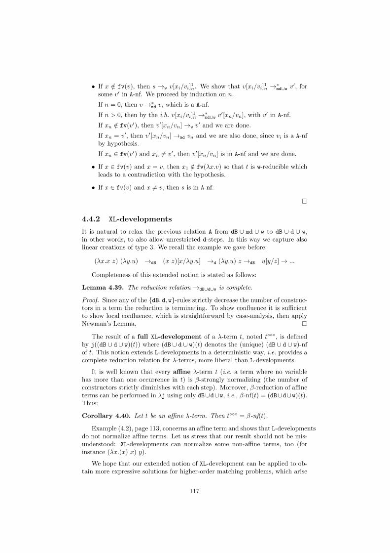
• If x /∈ fv(v), then s →w v[xi/vi]1n. We show that v[xi/vi]

1n →∗md∪w v′, for

some v′ in A-nf. We proceed by induction on n.

If n = 0, then v →∗md v, which is a A-nf.

If n > 0, then by the i.h. v[xi/vi]1n →∗md∪w v′[xn/vn], with v′ in A-nf.

If xn /∈ fv(v′), then v′[xn/vn]→w v′ and we are done.

If xn = v′, then v′[xn/vn]→md vn and we are also done, since vi is a A-nfby hypothesis.

If xn ∈ fv(v′) and xn 6= v′, then v′[xn/vn] is in A-nf and we are done.

• If x ∈ fv(v) and x = v, then x1 /∈ fv(λx.v) so that t is w-reducible whichleads to a contradiction with the hypothesis.

• If x ∈ fv(v) and x 6= v, then s is in A-nf.

4.4.2 XL-developments

It is natural to relax the previous relation A from dB ∪ md ∪ w to dB ∪ d ∪ w,in other words, to also allow unrestricted d-steps. In this way we capture alsolinear creations of type 3. We recall the example we gave before:

(λx.x z) (λy.u) →dB (x z)[x/λy.u] →d (λy.u) z →dB u[y/z]→ ...

Completeness of this extended notion is stated as follows:

Lemma 4.39. The reduction relation →dB∪d∪w is complete.

Proof. Since any of the dB, d, w-rules strictly decrease the number of construc-tors in a term the reduction is terminating. To show confluence it is sufficientto show local confluence, which is straightforward by case-analysis, then applyNewman’s Lemma.

The result of a full XL-development of a λ-term t, noted t, is definedby j((dB ∪ d ∪ w)(t)) where (dB ∪ d ∪ w)(t) denotes the (unique) (dB ∪ d ∪ w)-nfof t. This notion extends L-developments in a deterministic way, i.e. provides acomplete reduction relation for λ-terms, more liberal than L-developments.

It is well known that every affine λ-term t (i.e. a term where no variablehas more than one occurrence in t) is β-strongly normalizing (the number ofconstructors strictly diminishes with each step). Moreover, β-reduction of affineterms can be performed in λj using only dB∪d∪w, i.e., β-nf(t) = (dB∪d∪w)(t).Thus:

Corollary 4.40. Let t be an affine λ-term. Then t = β-nf(t).

Example (4.2), page 113, concerns an affine term and shows that L-developmentsdo not normalize affine terms. Let us stress that our result should not be mis-understood: XL-developments can normalize some non-affine terms, too (forinstance (λx.(x) x) y).

We hope that our extended notion of XL-development can be applied to ob-tain more expressive solutions for higher-order matching problems, which arise

117

for example in higher-order logic programming, logical frameworks, programtransformations, etc. Indeed, the approach of higher-order matching in untypedframeworks [Fau06, dMS01], which currently uses L-developments, may be im-proved using XL-developments, as suggested by example (4.2).

Let us conclude by discussing some further work on developments.

It is not clear to us whether the result of a full XL-developmentcan be de-fined by induction on t. Apparently not, but it may be possible to refine theapplication case in the inductive definition of L-developments into various sub-cases, exploiting the multiplicity of the abstracted variable, and catch theminductively.

One of the two axioms of the already cited notion of σ-equivalence (to beintroduced later on, Section 5.2, page 137) can also be seen as the equationalcharacterization of the relation having the same full 1-development on λ-terms(it is not proved in this thesis). More generally an interesting (future) com-plement of our work will be to find equational characterizations on λ-termsof the relations having the same full L-development and having the same fullXL-development.

In the literature developments are often defined with respect to a given setof redexes, and full developments are only a special case. It is natural to ask fora generalization of XL-developments to set of redexes. This certainly requires anheavy technical machinery in order to track along reductions only the redexes inthe set under observation plus those created by their reductions. This is why wepreferred to limit ourself to study notions of full developments. Our motivationwas to show the usefulness of the structural λ-calculus through an applicationat the rewriting theory of λ-calculus, so we preferred a less general notion anda lighter presentation.

118

Chapter 5

λj-dags, Pure Proof-Netsand σ-equivalence

In this chapter we introduce Regnier’s Pure Proof-Nets [Reg92] and study therelation between them and λj-dags, obtaining a full strong bisimulation, whichscales up to the structural λ-calculus. Along the way we show that the Danos-Regnier criterion for Pure Proof-Nets can be slightly simplified (lemma 5.16).

Then we reformulate Mascari and Pedicini’s Pure Proof-Nets linear headreduction [MP94] in λj in a clean way. We continue revisiting the notion ofσ-equivalence [Reg92, Reg94], which is a congruence introduced by Regnier onλ-calculus as the quotient (modulo multiplicative cuts) induced by Pure Proof-Nets on λ-terms. We conclude with the characterization of the quotient inducedby Pure Proof-Nets on the structural λ-calculus and on λj-dags.

Essentially, this chapter gives a solid justification to both λj-dags and thestructural λ-calculus: they are syntactic variations on the standard Linear Logicrepresentation of λ-calculus. On the other hand λj-dags and the structural λ-calculus can be seen as simplifications of Pure Proof-Nets: λj-dags abstract fromthe Linear Logic content, and the structural λ-calculus even makes unnecessaryto use a graphical syntax in order to understand and use Pure Proof-Nets.

The exact relation between λj-dags and Pure Proof-Nets and the characteri-zation of the quotients have been developed by the author alone. However, PureProof-Nets were the system inspiring λj-dags, and so they were underlying thejoint work of the author with Stefano Guerrini. And the new understandings oflinear head reduction and σ-equivalence are part of the joint work of the authorwith Delia Kesner.

5.1 Relating λj-dags and Pure Proof-Nets

In this section we relate our representation of λ-calculus with the standard call-by-name translation of λ-calculus into Pure Proof-Nets, which are a fragmentof Multiplicative Exponential Linear Logic extended with recursive types, in-troduced in [Reg92].

119

'

&

$

%

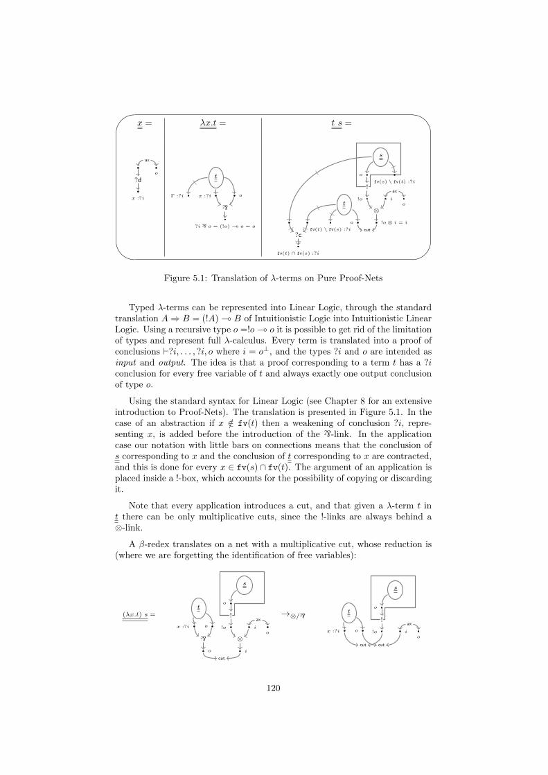
x = λx.t = t s =

o

ax

x :?i

?dt

ox :?i

?i ` o = (!o)( o = o

`

Γ :?i

t

fv(t) \ fv(s) :?i

o !o ⊗ i = i

i!o

⊗

o

!

o

ax

s

fv(s) \ fv(t) :?i

cut

fv(t) ∩ fv(s) :?i

?c

Figure 5.1: Translation of λ-terms on Pure Proof-Nets

Typed λ-terms can be represented into Linear Logic, through the standardtranslation A⇒ B = (!A)( B of Intuitionistic Logic into Intuitionistic LinearLogic. Using a recursive type o =!o( o it is possible to get rid of the limitationof types and represent full λ-calculus. Every term is translated into a proof ofconclusions `?i, . . . , ?i, o where i = o⊥, and the types ?i and o are intended asinput and output. The idea is that a proof corresponding to a term t has a ?iconclusion for every free variable of t and always exactly one output conclusionof type o.

Using the standard syntax for Linear Logic (see Chapter 8 for an extensiveintroduction to Proof-Nets). The translation is presented in Figure 5.1. In thecase of an abstraction if x /∈ fv(t) then a weakening of conclusion ?i, repre-senting x, is added before the introduction of the `-link. In the applicationcase our notation with little bars on connections means that the conclusion ofs corresponding to x and the conclusion of t corresponding to x are contracted,and this is done for every x ∈ fv(s) ∩ fv(t). The argument of an application isplaced inside a !-box, which accounts for the possibility of copying or discardingit.

Note that every application introduces a cut, and that given a λ-term t int there can be only multiplicative cuts, since the !-links are always behind a⊗-link.

A β-redex translates on a net with a multiplicative cut, whose reduction is(where we are forgetting the identification of free variables):

(λx.t) s =t

ox :?i

o

`

i

i!o

⊗

o

!

o

ax

s

cut

→⊗/` t

ox :?i i!o

o

!

o

ax

s

cut cut

120

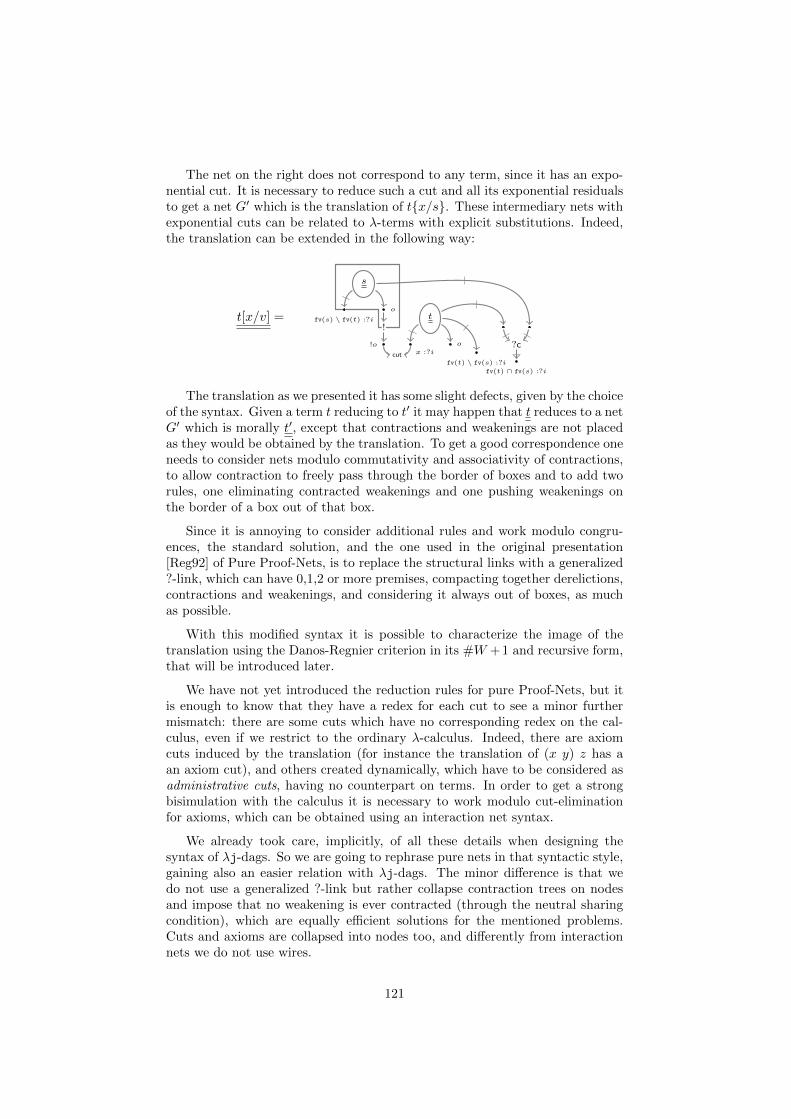
The net on the right does not correspond to any term, since it has an expo-nential cut. It is necessary to reduce such a cut and all its exponential residualsto get a net G′ which is the translation of tx/s. These intermediary nets withexponential cuts can be related to λ-terms with explicit substitutions. Indeed,the translation can be extended in the following way:

t[x/v] = t

x :?i

o!o

o

!

s

fv(s) \ fv(t) :?i

cutfv(t) \ fv(s) :?i

fv(t) ∩ fv(s) :?i

?c

The translation as we presented it has some slight defects, given by the choiceof the syntax. Given a term t reducing to t′ it may happen that t reduces to a netG′ which is morally t′, except that contractions and weakenings are not placedas they would be obtained by the translation. To get a good correspondence oneneeds to consider nets modulo commutativity and associativity of contractions,to allow contraction to freely pass through the border of boxes and to add tworules, one eliminating contracted weakenings and one pushing weakenings onthe border of a box out of that box.

Since it is annoying to consider additional rules and work modulo congru-ences, the standard solution, and the one used in the original presentation[Reg92] of Pure Proof-Nets, is to replace the structural links with a generalized?-link, which can have 0,1,2 or more premises, compacting together derelictions,contractions and weakenings, and considering it always out of boxes, as muchas possible.

With this modified syntax it is possible to characterize the image of thetranslation using the Danos-Regnier criterion in its #W +1 and recursive form,that will be introduced later.

We have not yet introduced the reduction rules for pure Proof-Nets, but itis enough to know that they have a redex for each cut to see a minor furthermismatch: there are some cuts which have no corresponding redex on the cal-culus, even if we restrict to the ordinary λ-calculus. Indeed, there are axiomcuts induced by the translation (for instance the translation of (x y) z has aan axiom cut), and others created dynamically, which have to be considered asadministrative cuts, having no counterpart on terms. In order to get a strongbisimulation with the calculus it is necessary to work modulo cut-eliminationfor axioms, which can be obtained using an interaction net syntax.

We already took care, implicitly, of all these details when designing thesyntax of λj-dags. So we are going to rephrase pure nets in that syntactic style,gaining also an easier relation with λj-dags. The minor difference is that wedo not use a generalized ?-link but rather collapse contraction trees on nodesand impose that no weakening is ever contracted (through the neutral sharingcondition), which are equally efficient solutions for the mentioned problems.Cuts and axioms are collapsed into nodes too, and differently from interactionnets we do not use wires.

121

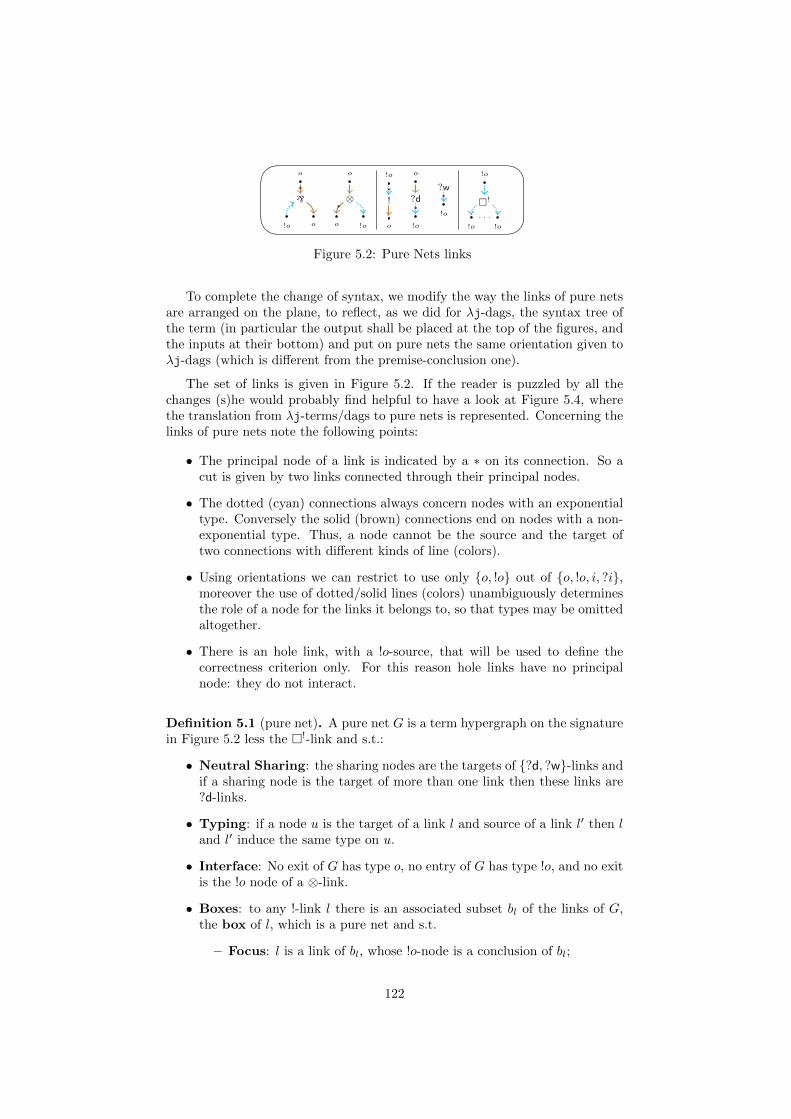
o

o!o

`*

o

!oo

⊗*

!o

o

!*

o

!o

?d*

!o

?w*

!o

!o!o

!

. . .

Figure 5.2: Pure Nets links

To complete the change of syntax, we modify the way the links of pure netsare arranged on the plane, to reflect, as we did for λj-dags, the syntax tree ofthe term (in particular the output shall be placed at the top of the figures, andthe inputs at their bottom) and put on pure nets the same orientation given toλj-dags (which is different from the premise-conclusion one).

The set of links is given in Figure 5.2. If the reader is puzzled by all thechanges (s)he would probably find helpful to have a look at Figure 5.4, wherethe translation from λj-terms/dags to pure nets is represented. Concerning thelinks of pure nets note the following points:

• The principal node of a link is indicated by a ∗ on its connection. So acut is given by two links connected through their principal nodes.

• The dotted (cyan) connections always concern nodes with an exponentialtype. Conversely the solid (brown) connections end on nodes with a non-exponential type. Thus, a node cannot be the source and the target oftwo connections with different kinds of line (colors).

• Using orientations we can restrict to use only o, !o out of o, !o, i, ?i,moreover the use of dotted/solid lines (colors) unambiguously determinesthe role of a node for the links it belongs to, so that types may be omittedaltogether.

• There is an hole link, with a !o-source, that will be used to define thecorrectness criterion only. For this reason hole links have no principalnode: they do not interact.

Definition 5.1 (pure net). A pure net G is a term hypergraph on the signaturein Figure 5.2 less the !-link and s.t.:

• Neutral Sharing: the sharing nodes are the targets of ?d, ?w-links andif a sharing node is the target of more than one link then these links are?d-links.

• Typing: if a node u is the target of a link l and source of a link l′ then land l′ induce the same type on u.

• Interface: No exit of G has type o, no entry of G has type !o, and no exitis the !o node of a ⊗-link.

• Boxes: to any !-link l there is an associated subset bl of the links of G,the box of l, which is a pure net and s.t.

– Focus: l is a link of bl, whose !o-node is a conclusion of bl;

122

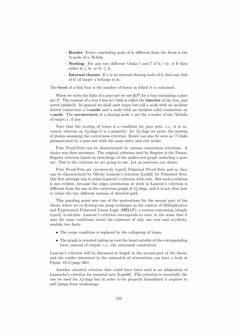
– Border: Every concluding node of bl different from the focus is the!o-node of a ?d-link;

– Nesting: For any two different !-links l and l′ if bl ∩ bl′ 6= ∅ theneither bl ⊆ bl′ or bl′ ⊆ bl.

– Internal closure: If u is an internal sharing node of bl then any linkof G of target u belongs to bl.

The level of a link/box is the number of boxes in which it is contained.

When we write the links of a pure net we use B[P ] for a box containing a purenet P . The content of a box b less its !-link is called the interior of the box, andnoted inter(b). In general we shall omit types but call a node with an incidentdotted connection a !o-node and a node with an incident solid connection ano-node. The occurrences of a sharing node x are the o-nodes of the ?d-linksof target x, if any.

Note that the nesting of boxes is a condition for pure nets, i.e., it is as-sumed, whereas on λj-dags it is a property: for λj-dags we prove the nestingof jboxes assuming the correctness criterion. Boxes can also be seen as !-linksparametrized by a pure net with the same entry and exit nodes.

Pure Proof-Nets can be characterized by various correctness criterions. Achoice was then necessary. The original criterion used by Regnier is the Danos-Regnier criterion based on switchings of the undirected graph underling a purenet. This is the criterion we are going to use. Let us motivate our choice.

Pure Proof-Nets are (recursively typed) Polarized Proof-Nets and so theycan be characterized by Olivier Laurent’s criterion [Lau02] for Polarized Nets.Our first attempt was to relate Laurent’s criterion with ours. But such a relationis not evident, because the edges orientation at work in Laurent’s criterion isdifferent from the one in the correction graph of λj-dags, and it is not clear howto relate the two different notions of directed path.

This puzzling point was one of the motivations for the second part of thethesis, where we re-develop our jump technique in the context of Multiplicativeand Exponential Polarized Linear Logic (MELLP), a system containing (simplytyped) λ-calculus. Laurent’s criterion corresponds to ours, in the sense that ituses the same conditions about the existence of only one root and acyclicity,modulo two facts:

• The scope condition is replaced by the collapsing of boxes.

• The graph is oriented taking as root the head variable of the correspondingterm, instead of output, i.e., the outermost constructor.

Laurent’s criterion will be discussed at length in the second part of the thesis,and the reader interested in the mismatch of orientations can have a look atFigure 10.3 (page 265).

Another oriented criterion that could have been used is an adaptation ofLamarche’s criterion for essential nets [Lam08]. This criterion is essentially theone we used for λj-dags but in order to be properly formulated it requires toadd jumps from weakenings.

123

'

&

$

%

o

o!o

`*

o

!oo

⊗*

o

!o

?d*

!o

?w*

!o

!o!o

!

. . .

o

o!o

o

!oo

o

!o

!o

o

!o!o

. . .

Figure 5.3: the edges of the undirect graph und(P 0)

But on one hand we did not like the idea of using both jumps and explicitboxes on Pure Nets (which is however a question of taste). And on the otherhand we wanted to better understand the relation between our criterion (orthe Lamarche criterion, if you prefer) and the Danos-Regnier criterion for tworeasons: first it is probably the most used criterion in the theory of Proof-Nets,and a thesis needs to confront the literature, and second because on a moretechnical level we wanted to better understand the relation between a criterionusing directed graphs and a criterion using undirected graphs, in particular themeaning of the scope condition for λj-dags in terms of switchings.

The relation between λj-dags and Lamarche-correct Pure Nets would cer-tainly be simpler than the one which shall follow, but the heavier treatmentinduced by the use of the Danos-Regnier criterion has the by-product of giv-ing us a precise characterization of the scope condition for λj-dags in terms ofswitching graphs and, a posteriori, a slight simplification of the Danos-Regniercriterion for Pure Nets (lemma 5.16).

Because of explicit boxes the definition of the Danos-Regnier criterion isslightly different from the one we used on λ-trees in Subsection 2.5.2 (page 43).

Definition 5.2 (switching graph). Let P be a pure net. We define P 0 asP where every box bl, with all its content, has been replaced with a !-linkl′ = 〈u|!|∆〉 where u is the o-node of l and ∆ is the set of exits of bl. Thenode u of l′ is an occurrence of every variable in ∆. The undirected graphund(P 0) of P 0 is the graph obtained from P by the transformation in Figure5.3. A switching S for P is a minimal set of nodes containing:

• One occurrence for every contracted sharing node x in P 0, and

• One among the body node (i.e., the target o-node) and the variable node(i.e., the source !o-node) for every `-link in P 0.

The switching S is principal if for every `-link it contains the target o-node.Given a switching S for P the switching graph P (S) is obtained from und(P 0)by:

• Removing every edge between x and its occurrences not in S, for everycontracted sharing node x;

• Removing the edge between the source o-node u and the node not in Samong x and v, for every `-link l = 〈u, x|`|v〉 in P 0 .

124

'

&

$

%

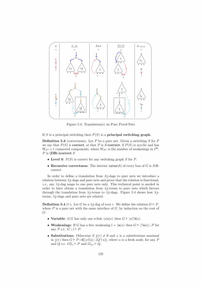
x s1 s2 λx.s t[x/s] tY]x

= = = = =

x

v

@

s2s1

Γ

s

x

λ t

x

s

Γ

j

tY

x

w

x

?d*

⊗*

!*

s2

s1

Γ

s

x

`*

t

x

!*

s

Γ

tY

x

?w*

Figure 5.4: Translation(s) on Pure Proof-Nets

If S is a principal switching then P (S) is a principal switching graph.

Definition 5.3 (correctness). Let P be a pure net. Given a switching S for Pwe say that P (S) is correct, or that P is S-correct, if P (S) is acyclic and hasWP 0 + 1 connected components, where WP 0 is the number of weakenings in P 0.P is (DR-)correct if

• Level 0: P (S) is correct for any switching graph S for P .

• Recursive correctness: The interior inter(b) of every box of G is DR-correct.

In order to define a translation from λj-dags to pure nets we introduce arelation between λj-dags and pure nets and prove that the relation is functional,i.e., any λj-dag maps to one pure nets only. This technical point is needed inorder to later obtain a translation from λj-terms to pure nets which factorsthrough the translation from λj-terms to λj-dags. Figure 5.4 shows how λj-terms, λj-dags and pure nets are related.

Definition 5.4 (). Let G be a λj-dag of root r. We define the relation G P ,where P is a pure net with the same interface of G, by induction on the root ofG:

• Variable: if G has only one v-link 〈u|v|x〉 then G 〈u|?d|x〉.

• Weakenings: If G has a free weakening l = 〈w|x〉 then G 〈?w|x〉 ;P forany P s.t. G \ l P .

• Substitutions: Otherwise if j(r) 6= ∅ and x is a substitutions maximalin j(r) then G P B[〈x|!|u〉 ; (Q † u)], where u is a fresh node, for any Pand Q s.t. G6↑x P and G↓x Q.

125

• Otherwise if the root link l is

– Application: An @-link 〈u|@|v, w〉 thenG 〈u|⊗|v, w′〉;PB[〈w′|!|w〉;Q], with w′ a fresh node, for any P and Q s.t. G↓v P and G↓w Q.

– Abstraction: A λ-link l = 〈u, x|λ|v〉 then G 〈u, x|`|v〉 ;P for anyP s.t. G \ l P .

It is immediate that the abstraction case can equivalently be defined withrespect to any P s.t. G↓v 〈w|x〉 P .

Note that the translation introduces a box for every application and a boxfor every substitution, while jumps are used only for substitutions. This meansthat if there is at least an application then there are less jumps in a λj-dag thanboxes in the corresponding pure net.

Definition 5.5 (Pure Proof-Net). Let P be a pure net. P is a pure proof-netif there is a λj-dag G s.t. G P .

Let us prove that is a functional relation.

Lemma 5.6. Let G be a λj-dag, P,Q pure nets s.t. G P and G Q. ThenP = Q.

Proof. By induction on the number of links in G. The only case which is notimmediate from the i.h. is the following. Suppose j(r) 6= ∅. If G P thenthere exists x maximal in j(r) s.t. P = P1 B[〈x|!|u〉 ; (P2 † u)] and G6↑x P1

and G↓x P2. Similarly, if G Q then there exists y maximal in j(r) s.t.Q = Q1 B[〈y|!|v〉 ; (Q2 † v)] and G6↑y Q1 and G↓y Q2. Then x is maximalin G6↑y so:

G6↑y Q3 B[〈x|!|u〉 ; (Q4 † u)]

With (G6↑y)6↑x Q3 and (G6↑y)↓x Q4. By i.h. we get Q1 = Q3 B[〈x|!|u〉 ; (Q4 †u)] and:

Q = Q3 B[〈x|!|u〉 ; (Q4 † u)] B[〈y|!|v〉 ; (Q2 † v)]

Similarly, y is maximal in G6↑x thus:

G6↑x P3 B[〈y|!|v〉 ; (P4 † v)]

With (G6↑x)6↑y P3 and (G6↑x)↓y P4. By i.h. we get P1 = P3B[〈y|!|v〉;(P4†v)]and:

P = P3 B[〈y|!|v〉 ; (P4 † v)] B[〈x|!|u〉 ; (P2 † u)]

By the nesting lemma G↓x and G↓y are disjoint (because none of them containsthe root link of the other) and since both x and y are maximal by lemma 3.15G can be written as:

(G′ G↓y G↓x) ; 〈rG′ |j|x〉 ; 〈rG′ |j|y〉

Then (G6↑y)↓x = G↓x, (G6↑x)↓y = G↓y and G′ = (G6↑y) 6↑x = (G6↑x) 6↑y. By thei.h. we get Q2 = P4, Q3 = P3 and Q4 = P2, i.e., P = Q.

Then given a λj-dag G we write G for the only pure net s.t. G G.

We can define a translation from λj-terms to Pure Nets.

126

Definition 5.7. Let t be a well-named λj-term. The translation tX

(noted t ifX = ∅) is defined by induction on t as follows:

x = 〈ux|?d|x〉λx.s = 〈x, uλx.s|`|us〉 ; s

x

s1 s2 = 〈us1s2 |⊗|us1 , v〉 ; (s1 B[〈v|!|us2〉 ; s2])

s1 [x/s2] = (s1x B[〈x|!|us2〉 ; s2])

tX]y = t

X 〈?w|y〉

The translation of λj-terms factors through the translation of λj-dags.

Lemma 5.8. Let t be a λj-term. Then tX

= (tX).

Proof. Straightforward induction on the definition of tX

.

We then write t P if t is a λj-term and P is a pure net s.t. tX

= P for aset of variables X.

Lemma 5.9. Let G be a λj-dag. Then G is DR-correct.

Proof. By induction on the translation. If j(r) 6= ∅ then let x be maximal inj(r). We have G = P = P ′ B[〈x|!|u〉 ; (Q † u)] with G6↑x = P ′ and G↓x = Q.

The nesting condition holds because by definition G6↑x and G↓x are disjoint.Let P (S) be a switching graph of P s. t. the switching S never chooses exitsof G↓x if it can. By lemma 3.15 the conclusions of G↓x are conclusions of G sothe !-link l replacing b = B[〈x|!|u〉 ; (Q † u)] contributes to P (S) with a set ofedges s.t. one of their extremities is a leaf of P (S) and the other is the nodex. Removing from P (S) the edges induced by l together with their leaf nodesthe number of connected components does not increases and no cycle is opened.By the choice of S the graph P (S) after the removal of the edges of l can beseen as a switching graph of P ′, which by i.h. is correct, so P (S) is correct.Any other switching graph P (S′) can be obtained from a switching having thesame property of S by switching on the occurrence of l for n nodes x1 . . . , xnamong the exits of G↓x which are the target of some v-link in G6↑x. We proveP (S′) correct by induction on n. The case n = 0 has already been treated. Ifn > 0 then consider the switch S′′ like S′ but for xn. By i.h. P (S′′) is correct.Then P (S′) is correct since the switch only changes the point where a leaf of theforest is attached and so choosing the occurrence of l no cycle can be creatednor the number of connected components can be altered. The interior of boxesare correct by i.h..For the application case the reasoning is analogous, the other cases are trivial.

5.1.1 Sequentialization

The aim of this subsection is to prove a sequentialization theorem of Pure Proof-Nets with respect to λj-dags, even if the terminology is slightly improper, sinceλj-dags are not sequential. By observing that the proof of the sequentializationtheorem requires only a particular kind of switching we shall slightly simplifythe Danos-Regnier criterion (lemma 5.16 at the end of this subsection).

127

To the reader not interested in correctness criterions we suggest to jump tothe next subsection (page 130) where the rewriting rules for Pure Proof-Netsare introduced.

We need some definitions and lemmas. With respect to the previous chapterswe speed up a bit, for instance we avoid the explicit definition of the read-back.

First of all note that the interface condition in the definition of pure netsimposes that the !o-node of a ⊗-link cannot be a conclusion of the net. Thisrequirement is equivalent to ask that there are no exponential axioms in theusual presentation of Pure Proof-Nets, which is part of the usual characterizationof λ-terms in terms of pure nets. This is needed to exclude configurations like:

⊗*

?d*

Which would not correspond to any λj-term/dag, despite being correct andwell-typed. Consequently, any ⊗-link has an associated box on its !o-node.Analogously, any exponential cut involves a box.

The first lemma shows that DR-correctness together with the impositionson the type of the interface implies the existence of exactly one entry node (inthe net not in the switching graphs) of the right kind.

Lemma 5.10. If P is a DR-correct pure net then it has only one entry noder, called the root, which is an o-node. Moreover, in every principal switchinggraph of P there is a path from r to every o-node of P 0.

Proof. Fix a principal switching S and consider P (S). By the shape of a prin-cipal switching graph every node u which is the target of a non-weakening linkl has exactly one incoming edge e defined by l whose other node is a source of l.So for every such node there is a notion of predecessor, and it is unique. ThenP (S) is a directed forest whose roots are weakenings and entry nodes. SinceP (S) has #W + 1 connected components there is exactly one entry node r. Bythe interface condition entry nodes are o-nodes, so r is an o-node.Given an o-node u and reconstructing backwards the path τ from its root wesee that τ passes through o-nodes only, since in P 0 there are no !-links. But ris the only root which is an o-node so τ is a path from r to u.

As for λj-dags we proceed by proving two splitting lemmas, for exponentialcuts and ⊗-links. In λj-dags we used a notion of maximality with respect to thepath order to prove that a substitution was splitting. On pure nets substitutionscorrespond to exponential cuts, and maximality is replaced by being special, aterm due to Regnier [Reg92] (page 43 of his thesis).

Definition 5.11 (special box/cut). Let P be a pure proof-net. A box is specialif it is at level 0 and all its exits are exits of P . An exponential cut is special ifits box is special.

Lemma 5.12 (special cut splitting). If P is a DR-correct pure net with aspecial exponential cut of box b. Then the net P ′ obtained by removing b fromP is DR-correct.

128

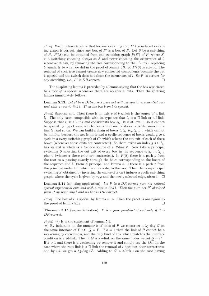
Proof. We only have to show that for any switching S of P ′ the induced switch-ing graph is correct, since any box of P ′ is a box of P . Let S be a switchingof P . P ′(S) can be obtained from one switching graph P (S′) of P , where S′

is a switching choosing always as S and never choosing the occurrence of l,whenever it can, by removing the tree corresponding to the !-link l replacingb, similarly to what we did in the proof of lemma 5.9. So P ′(S) is acyclic. Theremoval of such tree cannot create new connected components because the cutis special and the switch does not chose the occurrence of l. So P ′ is correct forany switching, i.e., P ′ is DR-correct.

The ⊗ splitting lemma is preceded by a lemma saying that the box associatedto a root ⊗ is special whenever there are no special cuts. Then the splittinglemma immediately follows.

Lemma 5.13. Let P be a DR-correct pure net without special exponential cutsand with a root ⊗-link l. Then the box b on l is special.

Proof. Suppose not. Then there is an exit v of b which is the source of a linkl1. The only cases compatible with its type are that l1 is a `-link or a !-link.Suppose that l1 is a !-link and consider its box bl1 . It is at level 0, so it cannotbe special by hypothesis, which means that one of its exits is the source of alink l2, and so on. We can build a chain of boxes b, bl1 , bl2 , bl3 , . . . which cannotbe infinite, because the net is finite and a cyclic sequence of boxes would give acycle in a every switching graph of G0 which selects the cut exit of each of theseboxes (whenever those exits are contracted). So there exists an index j s.t. bljhas an exit u which is a !o-node source of a `-link l′. Now take a principalswitching S selecting the cut exit of every box in the sequence b, bl1 , . . . blj−1

plus u (whenever these exits are contracted). In P (S) there is a path ρ fromthe root to u passing exactly through the holes corresponding to the boxes ofthe sequence and l. From S principal and lemma 5.10 there is a path τ fromthe principal node of l′, which is an o-node, to the root. Then the non-principalswitching S′ obtained by inverting the choice of S on l induces a cyclic switchinggraph, where the cycle is given by τ , ρ and the newly selected edge, absurd.

Lemma 5.14 (splitting application). Let P be a DR-correct pure net withoutspecial exponential cuts and with a root ⊗-link l. Then the pure net P ′ obtainedfrom P by removing l and its box is DR-correct.

Proof. The box of l is special by lemma 5.13. Then the proof is analogous tothe proof of lemma 5.12.

Theorem 5.15 (sequentialization). P is a pure proof-net if and only if it isDR-correct.

Proof. ⇒) It is the statement of lemma 5.9.⇐) By induction on the number k of links of P we construct a λj-dag G onthe same interface of P s.t. G = P . If k = 1 then the link of P cannot be aweakening by correctness, and the only kind of link which matches the interfacecondition is a ?d-link. Then if G is a v-link on the same nodes we get G = P .If k > 1 and there is a weakening we remove it and simply use the i.h.. In thecase where the root link is a `-link the removal of l does not alter correctness,and by i.h. we get a λj-dag G′. Adding to G′ a λ-link i on the root having

129

as variable x the !o-node of l we get a λj-dag, since by correctness of G′ andlemma 3.7 any term node of G′, and thus in particular the occurrences of x, hasa solid path from the root of G′, and so i verifies the scope condition.If P has a special cut l on a !o-node u then remove the involved box b. By lemma5.12 the obtained net P ′ is correct. By i.h. there is a λj-dag G′ translating toP ′ having in particular u as free sharing nodes. The i.h. applied to the interiorQ of the removed box, which is correct by the definition of correctness by levels,gives a λj-dag H mapping to Q. Then we define G as (G′ (H † u)) ; 〈rG′ |j|u〉.The correctness of G′ and H directly implies the rooted dag condition for G,and the scope condition for every jump except the new one. By lemma 3.7 anyterm node of G′, and thus in particular the occurrences of u, has a solid pathfrom the root, so the scope condition for the jump holds. The fact that theremoved cut is special implies that u is a maximal substitution in j(rG), and soG = PThe only case left is that the root link is a ⊗-link l and that there is no specialcut. Then by lemma 5.14 the net P ′ obtained from P by removing l and its boxb is DR-correct. Putting an application on the top of the λj-dags given by thei.h. for P ′ and for the interior of b, we get a λj-structure G whose correctnessimmediately follows from the i.h.. By definition of translation G = P .

In the proof of lemma 5.13 we used almost principal switchings, a very specialform of non-principal switching, having exactly one λ-link in a non-principalposition, as in subsection 2.5.2 (page 43). Since this is the only point wherenon-principal switching are used we get that the DR-criterion can be simplifiedin the case of pure nets, too:

Lemma 5.16. Let G be a λ-structure. G is correct if and only if it is S-correctwith respect to any principal switching and any almost principal switching.

Moreover, we have the following corollary:

Corollary 5.17. If P is a Pure Proof-Net then there exist a λj-term t and aset of variables X s.t. t

X= P .

Proof. By the sequentialization theorems from Pure Proof-Nets to λj-dags andfrom λj-dags to λj-term and the fact that ·

Xis defined as the composition of

the two respective translations.

5.1.2 Dynamics

The reduction rules for Pure Proof-Nets are in figure 5.5. In Regnier’s thesis[Reg92] Pure Proof-Nets are endowed with just one exponential rule, similar tothe meta-substitution we defined for λ-trees, making all the copies of the boxand then opening them (or erasing the box in the case of a weakening). Weprefer a decomposed presentation because it is closer to λj-dags, we commenton our choice at the end of the section.

The rules are the exact analogous of the rules for λj-dags without the jumps.The multiplicative rule is better understood if we also represent a part of itscontext:

130

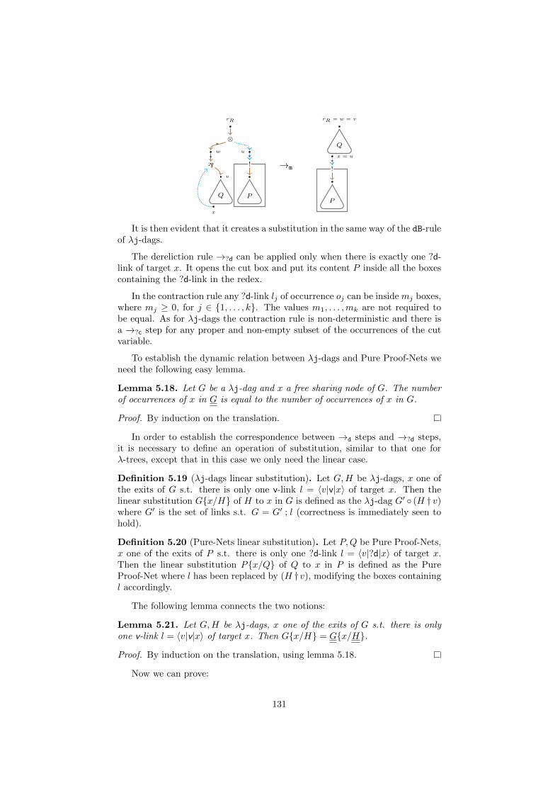
rR

w u

⊗*

!*

P

v

Q

x

`*

→m

rR = w = v

Q

x = u

!*

P

It is then evident that it creates a substitution in the same way of the dB-ruleof λj-dags.

The dereliction rule →?d can be applied only when there is exactly one ?d-link of target x. It opens the cut box and put its content P inside all the boxescontaining the ?d-link in the redex.

In the contraction rule any ?d-link lj of occurrence oj can be inside mj boxes,where mj ≥ 0, for j ∈ 1, . . . , k. The values m1, . . . ,mk are not required tobe equal. As for λj-dags the contraction rule is non-deterministic and there isa →?c step for any proper and non-empty subset of the occurrences of the cutvariable.

To establish the dynamic relation between λj-dags and Pure Proof-Nets weneed the following easy lemma.

Lemma 5.18. Let G be a λj-dag and x a free sharing node of G. The numberof occurrences of x in G is equal to the number of occurrences of x in G.

Proof. By induction on the translation.

In order to establish the correspondence between →d steps and →?d steps,it is necessary to define an operation of substitution, similar to that one forλ-trees, except that in this case we only need the linear case.

Definition 5.19 (λj-dags linear substitution). Let G,H be λj-dags, x one ofthe exits of G s.t. there is only one v-link l = 〈v|v|x〉 of target x. Then thelinear substitution Gx/H of H to x in G is defined as the λj-dag G′ (H † v)where G′ is the set of links s.t. G = G′ ; l (correctness is immediately seen tohold).

Definition 5.20 (Pure-Nets linear substitution). Let P,Q be Pure Proof-Nets,x one of the exits of P s.t. there is only one ?d-link l = 〈v|?d|x〉 of target x.Then the linear substitution Px/Q of Q to x in P is defined as the PureProof-Net where l has been replaced by (H †v), modifying the boxes containingl accordingly.

The following lemma connects the two notions:

Lemma 5.21. Let G,H be λj-dags, x one of the exits of G s.t. there is onlyone v-link l = 〈v|v|x〉 of target x. Then Gx/H = Gx/H.

Proof. By induction on the translation, using lemma 5.18.

Now we can prove:

131

'

&

$

%

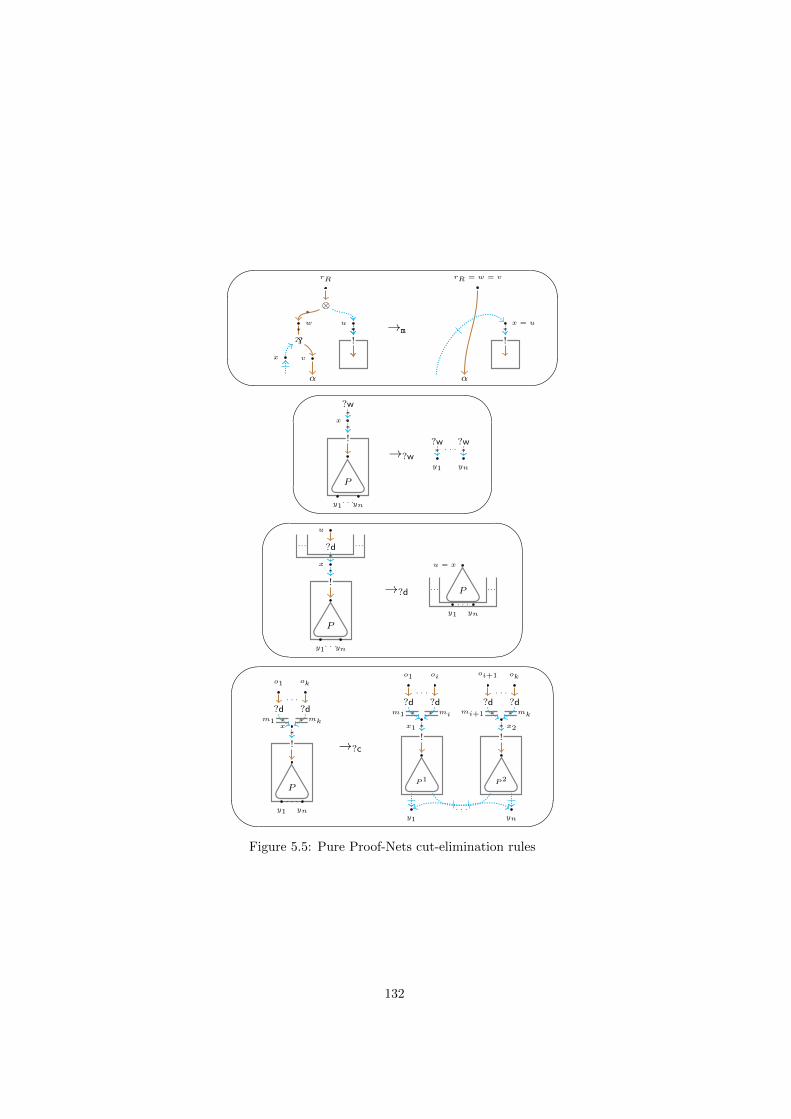
rR

w u

⊗*

!*

v

α

x

`*

!* →m

rR = w = v

x = u

α

!*

'

&

$

%

x

?w*

!*

P

y1 yn. . .

→?wy1 yn

?w*

?w*

. . .

'

&

$

%

u

x

?d*

!*

P

y1 yn. . .

... ...

→?d

u = x

P

y1 yn

. . .

... ...

'

&

$

%

o1 ok

. . .

x

?d*

?d*

!*

P

y1 yn

. . .

m1 mk

→?c

oio1 oi+1 ok

. . . . . .

x1

?d*

?d*

x2

?d*

?d*

!*

!*

P1 P2

y1 yn

. . .

m1 mi mi+1 mk

Figure 5.5: Pure Proof-Nets cut-elimination rules

132

Theorem 5.22 (strong bisimulation). The translation from λj-dags to PureProof-Nets is a full strong bisimulation. Moreover, if G P and G→a G

′ thenthere exists a unique Pure Proof-Net P ′ s.t. G′ P ′.

Proof. The proof is by induction on the translation, along the lines of the proofswe did for λj-trees and λj-dags. For all cases except the→?d /→d one the rulesfor pure proof-nets are exactly the same than those for λj-dags without jumpsand with boxes, and the translation does exactly that: it removes the jumpsand adds the boxes. A look at the rules and the translation is more convincingof the long technical unfolding of the definitions.The→?d /→d case is not difficult, however, it just involves the crossing of someexplicit boxes. It is enough to use the previous linear substitution lemma. Itfollows.Suppose that G is a λj-dag having a maximal substitution x anchored on theroot, target of only one v-link l = 〈v|v|x〉. Then G = G6↑xG↓x ;〈r|j|x〉. The→d

reduct of G is G6↑xx/H. The translation of G is G = G6↑x B[〈x|!|u〉(G↓x †u)],

which reduces to P ′ = G6↑xx/(G↓x†u) = G6↑xx/G↓x, where the last equality

is justified by the fact that the definition of linear substitution changes the rootof the argument of the substitution. By lemma 5.21 we get P ′ = G′.It is easily seen that the only redex not given by the i.h. is the treated one. Theunicity of P ′ is proved as in theorem 3.49 (page 80).

It is easy to see that the strong bisimulation between λj-dags and PureProof-Nets actually enjoys a bijection of one-step reductions, as it was the casefor the relation λ-terms/λ-trees, and in contrast to the relation λj-terms/λj-dags.

Note that we did not prove that correctness of pure-nets is preserved byreduction, but as in the case of λ-terms and λ-trees it follows from the fact thatthe reduct of a Pure Proof-Net can be seen as the translation of a λj-dag andthe fact that the translation of a λj-dag is a correct Pure Net.

Corollary 5.23. The translation from λj-terms to Pure Proof-Nets is a fullstrong bisimulation.

Proof. Simple calculation of the composition of the strong bisimulation betweenλj-terms and λj-dags (prop. 3.49, page 80) with the strong bisimulation be-tween λj-dags and Pure Proof-Nets (theorem 5.22).

Since the relation λj-terms/λj-dags does not enjoy a bijection on one-stepreductions we get that the relation λj-terms/Pure Proof-Nets does not enjoysuch a bijection, too.

Corollary 5.24. Pure Proof-Nets are confluent and enjoy the PSN property.

Proof. Confluence follows by lemma 3.56 (page 85) and the fact that the transla-tion from term to nets is a full strong bisimulation between λj-terms and PureProof-Nets enjoying with the unicity property required by the lemma. FromCorollaries 4.28 (page 108) and 3.54 (page 84) we also get PSN.

Note that the rule of traditional ES-calculi creating substitutions withoutdistance, i.e., (λx.t) u→B t[x/u] can be forced on λj-dags by asking that thereis no jump anchored on the source node of the λ-link, but there is no local way

133

of forcing such rule on pure proof-nets. Indeed, if M = (λx.t)L u then in Mthe explicit boxes corresponding to L are completely delocalized with respect tothe multiplicative cut corresponding to the dB-redex. More precisely, the netswould simulate the B-rule, but that rule does not simulate the multiplicativerule of Pure Proof Nets.

Curiously, in the Proof-Net literature there are mainly two syntaxes forexponentials, paired with two very different operational semantics. The first one,presented in Chapter 8, can be traced back to Girard [Gir87], where boxes canclose on weakenings, there is a commutative box-box rule and duplications aremade one at the time. The second one, introduced by Regnier’s [Reg92] to geta good representation of λ-calculus, uses generalized ?-links grouping togetherweakening, dereliction and contraction, boxes cannot close on weakenings, andthere is only one exponential rule, a big-steps rule making all the copies of thebox at once (and opening them).

The two are very different from an operational point of view. In termsof explicit substitutions Regnier’s operational semantics corresponds to have acalculus with only two rules:

(dB) (λx.t)L u → t[x/u]L(j) t[x/u] → tx/u

While Girard’s syntax would correspond to λj plus two rules,→ab and→sb,representing the box-box rule (this calculus is studied in Chapter 6):

(dB) (λx.t)L u → t[x/u]L(w) t[x/u] → t if |t|x = 0(d) t[x/u] → tx/u if |t|x = 1(c) t[x/u] → t[y]x [x/u][y/u] if |t|x ≥ 2

(ab) (t v)[x/u] → t v[x/u] x /∈ fv(t) & x ∈ fv(v)(sb) t[y/v][x/u] → t[y/v[x/u]] x /∈ fv(t) & x ∈ fv(v)

Actually, this set of rules is not really faithful to Girard’s operational seman-tics, since the rules of λj reduce through box borders (w and d in particular)while in Girard’s syntax it is necessary to go through one box at the time, usingthe rules corresponding to ab and sb. The calculus matching Girard’s semanticsis difficult to formulate, because it uses propagations and distance at the sametime, but the two are not independent.

Regnier’s style syntax is a big-steps cut-elimination semantics without prop-agations (commutative cut-elimination cases). Girard’s style is a small-stepssemantics with propagations. There is a choice in between, a small-steps seman-tics without propagations, the one presented here and corresponding exactly toλj, which seems to have never been considered before, with the partial excep-tion of [MP94] where the authors consider only a specific strategy, linear headreduction, that can be seen as a strategy of our semantics because it is a small-steps strategy that never needs to reduce through box borders, and so it isindependent from the commutative box-box rule.

Let us discuss it.

134

5.1.3 Linear head reduction

We need two definitions.

Definition 5.25 (head variable/context). The head variable occurrencehoc(t) of a λj-term t is defined by induction on t:

• hoc(x) = x;

• hoc(v u) = hoc(v)

• hoc(λx.v) = hoc(v)

• hoc(v[x/u]) = hoc(v)

An head context H[·] is a context where the hole has the position of the headvariable occurrence. A head context is capturing if it can capture the freevariables of what shall replace the hole, otherwise it is non-capturing.

An easy induction on the pure translation shows that hoc(t) is the only vari-able occurrence of t out of all boxes, since boxes are used to code the argumentof applications and the content of substitutions.

The fundamental property of hoc(t) is that it cannot be duplicated norerased, exactly because it is out of all boxes. In particular, since it cannotbe erased, any redex involving hoc(t) is needed, in the sense that it must becontracted in any reduction to normal form. There is an interesting strategy ofpure proof nets, the so-called linear head reduction (introduced by Mascariand Pedicini in [MP94]), which consists in reducing always the redex on thehead variable, if any. It is a deterministic and history-free strategy, since thereis always at most one head variable occurrence and its definition does not dependon the history of the reduction.

Through the strong bisimulation of Pure Proof-Nets with λj we can formu-late linear head reduction using the following root cases, where the head contextH[·] is intended as non-capturing:

If t = (λx.H[x])L v then t 7→hoc H[x][x/v]L.

If t = H[x][x/v] and |H[x]|x = 1 then t 7→hoc H[v].

If t = H[x][x/v] and |H[x]|x > 1 then t 7→hoc H[y][y/v][x/v].

Then the head linear rewriting relation →hoc is the closure of 7→hoc bycapturing head contexts. It is easily seen that this correspond exactly to whathappens in Pure Proof-Nets.

A corollary of PSN for λj is that our formulation →hoc is normalizing onall strong normalizing λ-terms. This is yet another example of useful exchangebetween the theory of explicit substitutions an the theory of Proof-Nets.

Danos and Regnier have studied this strategy in connection to the geometryof interaction and abstract machines [DR96], and together with Hugo Herbelinalso in relation to game semantics [DHR96]. However, their definition [DR04]is sensibly more complex than ours, because they used λ-calculus instead thanλj (that clearly did not exist at that time). We do not formally introduce their

135

notion, just give an example taken from [DR04]. First consider the head linearreduction of δ δ in our formulation:

(λx.x x) λy.y y →hoc (x x)[x/λy.y y] →hoc

(z x)[z/λy.y y][x/λy.y y] →hoc

((λy.y y) x)[x/λy.y y] →hoc

(y y)[y/x][x/λy.y y] →hoc

(z y)[z/x][y/x][x/λy.y y] →hoc . . .

Where the underlinings stress the current redex. Then let us explain howthey dealt with it. Since in λ-calculus there are no explicit substitutions if onewould have something finer than β-reduction is obliged to reduce as follows:

(λx.x x) λy.y y → (λx.(λy.y y) x) λy.y y

Let us explain what happened. The argument of the linear head redex hasbeen copied, and put at the place of the head variable, but the original redexhas not been eliminated. One can continue following this principle:

(λx.x x) λy.y y → (λx.(λy′.y′ y′) x) λy.y y →

(λx.(λy′.x y′) x) λy.y y →

(λx.(λy′.(λy′′.y′′ y′′) y′) x) λy.y y → . . .

Essentially their way of formulating linear head reduction consists in ex-panding explicit substitutions into β-redexes, but the fact that β-redexes arereduced in a way which is not β-reduction implies that this form of linear headreduction is not a reduction of λ-calculus, at least not in the usual sense.

A minor mismatch between nets and the Danos and Regnier reduction con-cerns the use of the arguments. The nets do not always keep a copy of theargument. For instance pure nets would reduce (λx.x) y to y in two steps whileDanos and Regnier linear reduction would reduce such term to (λx.y) y even ifthe argument is then useless. The behavior of their notion more closely corre-sponds to the operational semantics of Milner’s calculus (subsection 3.6.1, page82). However, this is just a detail.

More important, instead, is that Danos and Regnier’s formulation of linearhead reduction requires to define the linear head redex modulo a congruence, theso-called σ-equivalence (which is the subject of the next section). Consequently,Danos and Regnier’s formulation is quite difficult to manage.

Let us conclude by stressing that once more the structural λ-calculus can beused as a tool to study, re-understand and divulge existing notions of the theoryof λ-calculus. We believe that through λj the connection of linear head reduc-tion with game semantics, abstract machines and the geometry of interactionshould be revisited. In their current form these connections are extremely hard

136

to grasp, and we are confident that λj can be used to simplify them. There alsoexists a link between linear head reduction and the call-by-name translation ofλ-calculus into the π-calculus [Maz03], which would probably be interesting torevisit.

Finally, in future work we would like to develop results about linear headnormal forms in analogy to what has been done for head normal forms in λ-calculus.

5.2 σ-equivalence

In the next section we shall characterize the quotients induced on λj-terms andλj-dags by the translation on Pure Proof-Nets. Such quotients can be tracedback to a notion, σ-equivalence, introduced by Regnier [Reg92, Reg94], that weprefer to present before the technical details concerning the characterization ofthe quotients. Through λj we shall reformulate σ-equivalence as an equivalenceon substitutions having better properties than its formulation in the λ-calculus.

One of the nice features of graphical syntaxes is that usually they quotienta sequential language with respect to some permutation of constructors. Unfor-tunately, if Pure Proof-Nets are meant to represent ordinary λ-terms only (i.e.,without explicit substitutions) then the translation is injective, and there is noinduced quotient. This is the exact analogous of what happens with λ-trees.

In our context we can understand Regnier’s σ-equivalence as a way to re-cover a quotient from the translation of λ-terms on Pure Proof-Nets. Sometimesstarting with two nets P and Q corresponding to two different λ-terms and elim-inating the multiplicative cuts only (without reducing the created exponentialcuts) it happens that one gets the same net P ′ = Q′. Actually, in his thesisRegnier defines the translation this way, that is, he takes as translation t∗ of aλ-term t the net resulting from our t after the elimination of all multiplicativecuts. He defines σ-equivalence as the equivalence on λ-terms induced by thismodified translation. The equations defining Regnier’s σ-equivalence are:

(λx.λy.t) u ∼σR1 λy.((λx.t) u) if y /∈ fv(u)

(λx.t v) u ∼σR2 (λx.t) u v if x /∈ fv(v)

Let ≡σR ,≡σR1 ,≡σR2 be the equivalences generated by the context and tran-sitive closure of ∼σR1 ∪ ∼σR2 , ∼σR1 and ∼σR2 , respectively.

Regnier proved that two ≡σR -equivalent terms have essentially the sameoperational behavior: ≡σR is contained in the equational theory generated byβ-reduction, i.e., ≡σR⊂≡β , and if t ≡σR t′ then t and t′ have the same length ofa maximal β-reduction (the so-called Barendregt’s norm), and the same resultabout length of reductions is true with respect to left and head reduction.

For this strong property he calls ≡σR an operational equivalence. One wouldexpect that the result about length of reductions can be reformulated locally asa strong bisimulation, which would mean to have a property of this form:

t → u t → u≡σR ⇒ ≡σR ≡σRt′ t′ → u′

137

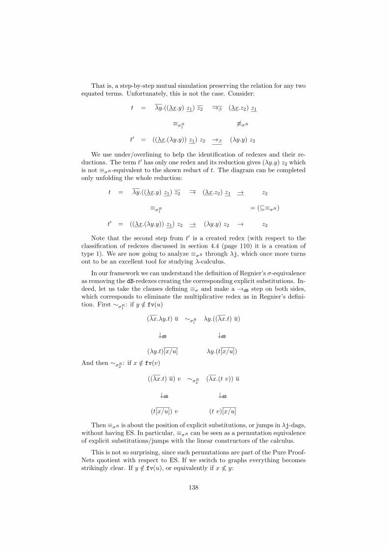
That is, a step-by-step mutual simulation preserving the relation for any twoequated terms. Unfortunately, this is not the case. Consider:

t = λy.((λx.y) z1) z2 →β (λx.z2) z1

≡σR1 6≡σR

t′ = ((λx.(λy.y)) z1) z2 →β (λy.y) z2

We use under/overlining to help the identification of redexes and their re-ductions. The term t′ has only one redex and its reduction gives (λy.y) z2 whichis not ≡σR -equivalent to the shown reduct of t. The diagram can be completedonly unfolding the whole reduction:

t = λy.((λx.y) z1) z2 → (λx.z2) z1 → z2

≡σR1 = (⊆≡σR)

t′ = ((λx.(λy.y)) z1) z2 → (λy.y) z2 → z2

Note that the second step from t′ is a created redex (with respect to theclassification of redexes discussed in section 4.4 (page 110) it is a creation oftype 1). We are now going to analyze ≡σR through λj, which once more turnsout to be an excellent tool for studying λ-calculus.

In our framework we can understand the definition of Regnier’s σ-equivalenceas removing the dB-redexes creating the corresponding explicit substitutions. In-deed, let us take the clauses defining ≡σ and make a →dB step on both sides,which corresponds to eliminate the multiplicative redex as in Regnier’s defini-tion. First ∼σR1 : if y /∈ fv(u)

(λx.λy.t) u ∼σR1 λy.((λx.t) u)

↓dB ↓dB

(λy.t)[x/u] λy.(t[x/u])

And then ∼σR2 : if x /∈ fv(v)

((λx.t) u) v ∼σR2 (λx.(t v)) u

↓dB ↓dB

(t[x/u]) v (t v)[x/u]

Then ≡σR is about the position of explicit substitutions, or jumps in λj-dags,without having ES. In particular, ≡σR can be seen as a permutation equivalenceof explicit substitutions/jumps with the linear constructors of the calculus.

This is not so surprising, since such permutations are part of the Pure Proof-Nets quotient with respect to ES. If we switch to graphs everything becomesstrikingly clear. If y /∈ fv(u), or equivalently if x 66 y:

138

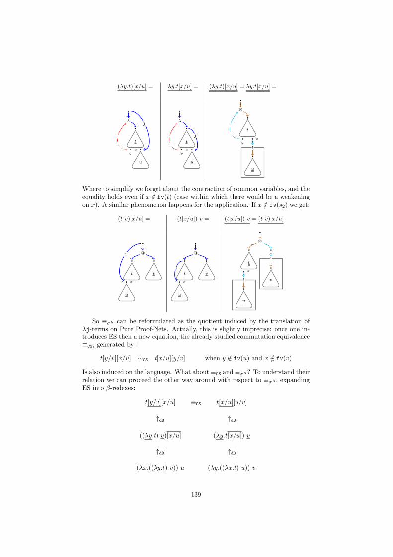
(λy.t)[x/u] = λy.t[x/u] = (λy.t)[x/u] = λy.t[x/u] =

t

y

λ

x

u

j

t

y

λ

x

u

jt

yx

`*

!*

u

Where to simplify we forget about the contraction of common variables, and theequality holds even if x /∈ fv(t) (case within which there would be a weakeningon x). A similar phenomenon happens for the application. If x /∈ fv(s2) we get:

(t v)[x/u] = (t[x/u]) v = (t[x/u]) v = (t v)[x/u]

@

vt

x

u

j @

vt

x

u

j

⊗*

!*

v

t

x

!*

u

So ≡σR can be reformulated as the quotient induced by the translation ofλj-terms on Pure Proof-Nets. Actually, this is slightly imprecise: once one in-troduces ES then a new equation, the already studied commutation equivalence≡CS, generated by :

t[y/v][x/u] ∼CS t[x/u][y/v] when y /∈ fv(u) and x /∈ fv(v)

Is also induced on the language. What about ≡CS and ≡σR? To understand theirrelation we can proceed the other way around with respect to ≡σR , expandingES into β-redexes:

t[y/v][x/u] ≡CS t[x/u][y/v]

↑dB ↑dB

((λy.t) v)[x/u] (λy.t[x/u]) v

↑dB ↑dB

(λx.((λy.t) v)) u (λy.((λx.t) u)) v

139

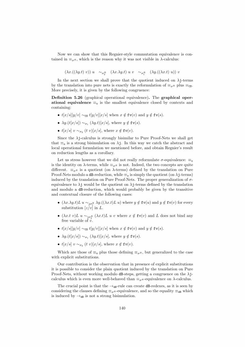
Now we can show that this Regnier-style commutation equivalence is con-tained in ≡σR , which is the reason why it was not visible in λ-calculus:

(λx.((λy.t) v)) u ∼σR2 (λx.λy.t) u v ∼σR1 (λy.((λx.t) u)) v

In the next section we shall prove that the quotient induced on λj-termsby the translation into pure nets is exactly the reformulation of ≡σR plus ≡CS.More precisely, it is given by the following congruence:

Definition 5.26 (graphical operational equivalence). The graphical oper-ational equivalence ≡o is the smallest equivalence closed by contexts andcontaining:

• t[x/s][y/v] ∼CS t[y/v][x/s] when x /∈ fv(v) and y /∈ fv(s).

• λy.(t[x/s]) ∼σ1(λy.t)[x/s], where y /∈ fv(s).

• t[x/s] v ∼σ2(t v)[x/s], where x /∈ fv(v).

Since the λj-calculus is strongly bisimilar to Pure Proof-Nets we shall getthat ≡o is a strong bisimulation on λj. In this way we catch the abstract andlocal operational formulation we mentioned before, and obtain Regnier’s resulton reduction lengths as a corollary.

Let us stress however that we did not really reformulate σ-equivalence: ≡o

is the identity on λ-terms, while ≡σR is not. Indeed, the two concepts are quitedifferent. ≡σR is a quotient (on λ-terms) defined by the translation on PureProof-Nets modulo a dB-reduction, while≡o is simply the quotient (on λj-terms)induced by the translation on Pure Proof-Nets. The proper generalization of σ-equivalence to λj would be the quotient on λj-terms defined by the translationand modulo a dB-reduction, which would probably be given by the transitiveand contextual closure of the following cases:

• (λx.λy.t)L u ∼jσR1λy.((λx.t)L u) where y /∈ fv(u) and y /∈ fv(v) for every

substitution [z/v] in L.

• (λx.t v)L u ∼jσR2(λx.t)L u v where x /∈ fv(v) and L does not bind any

free variable of v.

• t[x/s][y/v] ∼CS t[y/v][x/s] when x /∈ fv(v) and y /∈ fv(s).

• λy.(t[x/s]) ∼σ1(λy.t)[x/s], where y /∈ fv(s).

• t[x/s] v ∼σ2 (t v)[x/s], where x /∈ fv(v).

Which are those of ≡o plus those defining ≡σR , but generalized to the casewith explicit substitutions.

Our contribution is the observation that in presence of explicit substitutionsit is possible to consider the plain quotient induced by the translation on PureProof-Nets, without working modulo dB-steps, getting a congruence on the λj-calculus which is even more well-behaved than ≡σR -equivalence on λ-calculus.

The crucial point is that the →dB-rule can create dB-redexes, as it is seen byconsidering the clauses defining ≡σR -equivalence, and so the equality ≡dB whichis induced by →dB is not a strong bisimulation.

140

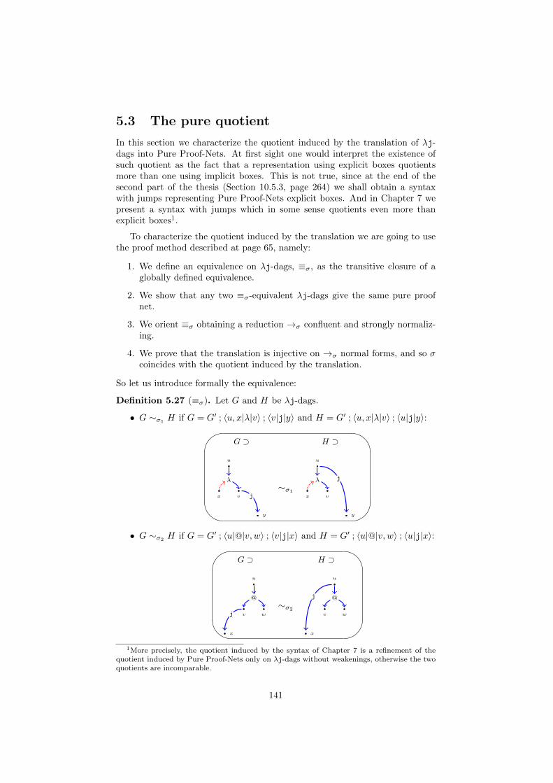
5.3 The pure quotient

In this section we characterize the quotient induced by the translation of λj-dags into Pure Proof-Nets. At first sight one would interpret the existence ofsuch quotient as the fact that a representation using explicit boxes quotientsmore than one using implicit boxes. This is not true, since at the end of thesecond part of the thesis (Section 10.5.3, page 264) we shall obtain a syntaxwith jumps representing Pure Proof-Nets explicit boxes. And in Chapter 7 wepresent a syntax with jumps which in some sense quotients even more thanexplicit boxes1.

To characterize the quotient induced by the translation we are going to usethe proof method described at page 65, namely:

1. We define an equivalence on λj-dags, ≡σ, as the transitive closure of aglobally defined equivalence.

2. We show that any two ≡σ-equivalent λj-dags give the same pure proofnet.

3. We orient ≡σ obtaining a reduction →σ confluent and strongly normaliz-ing.

4. We prove that the translation is injective on →σ normal forms, and so σcoincides with the quotient induced by the translation.

So let us introduce formally the equivalence:

Definition 5.27 (≡σ). Let G and H be λj-dags.

• G ∼σ1H if G = G′ ; 〈u, x|λ|v〉 ; 〈v|j|y〉 and H = G′ ; 〈u, x|λ|v〉 ; 〈u|j|y〉:'

&

$

%

G ⊃ H ⊃

u

x v

λ

y

j∼σ1

u

x v

λ

y

j

• G ∼σ2H if G = G′ ; 〈u|@|v, w〉 ; 〈v|j|x〉 and H = G′ ; 〈u|@|v, w〉 ; 〈u|j|x〉:'

&

$

%

G ⊃ H ⊃

u

v w

@

x

j∼σ2

u

v w

@

x

j

1More precisely, the quotient induced by the syntax of Chapter 7 is a refinement of thequotient induced by Pure Proof-Nets only on λj-dags without weakenings, otherwise the twoquotients are incomparable.

141

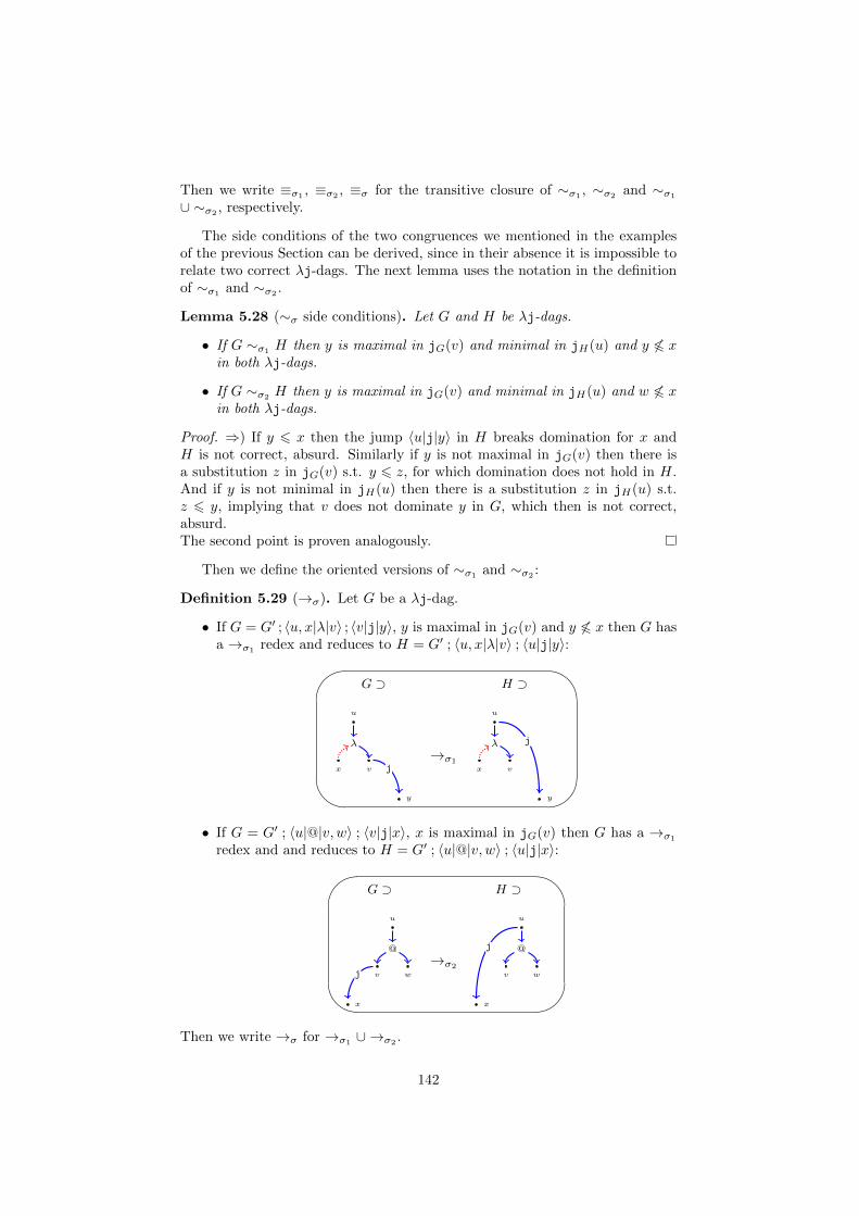
Then we write ≡σ1, ≡σ2

, ≡σ for the transitive closure of ∼σ1, ∼σ2

and ∼σ1

∪ ∼σ2, respectively.

The side conditions of the two congruences we mentioned in the examplesof the previous Section can be derived, since in their absence it is impossible torelate two correct λj-dags. The next lemma uses the notation in the definitionof ∼σ1 and ∼σ2 .

Lemma 5.28 (∼σ side conditions). Let G and H be λj-dags.

• If G ∼σ1 H then y is maximal in jG(v) and minimal in jH(u) and y 66 xin both λj-dags.

• If G ∼σ2H then y is maximal in jG(v) and minimal in jH(u) and w 66 x

in both λj-dags.

Proof. ⇒) If y 6 x then the jump 〈u|j|y〉 in H breaks domination for x andH is not correct, absurd. Similarly if y is not maximal in jG(v) then there isa substitution z in jG(v) s.t. y 6 z, for which domination does not hold in H.And if y is not minimal in jH(u) then there is a substitution z in jH(u) s.t.z 6 y, implying that v does not dominate y in G, which then is not correct,absurd.The second point is proven analogously.

Then we define the oriented versions of ∼σ1and ∼σ2

:

Definition 5.29 (→σ). Let G be a λj-dag.

• If G = G′ ; 〈u, x|λ|v〉 ; 〈v|j|y〉, y is maximal in jG(v) and y 66 x then G hasa →σ1 redex and reduces to H = G′ ; 〈u, x|λ|v〉 ; 〈u|j|y〉:'

&

$

%

G ⊃ H ⊃

u

x v

λ

y

j→σ1

u

x v

λ

y

j

• If G = G′ ; 〈u|@|v, w〉 ; 〈v|j|x〉, x is maximal in jG(v) then G has a →σ1

redex and and reduces to H = G′ ; 〈u|@|v, w〉 ; 〈u|j|x〉:'

&

$

%

G ⊃ H ⊃

u

v w

@

x

j→σ2

u

v w

@

x

j

Then we write →σ for →σ1∪ →σ2

.

142

The reductions →σ1and →σ2

preserve correctness.

Lemma 5.30 (→σ preserve correctness). Let G be a λj-dag. If G→σ H thenH is a λj-dag.

Proof. Root : both rules clearly do not create nor destroy initial nodes.Acyclicity : The new edge in H cannot close a cycle because there is a coinitialand cofinal path in G, and G is acyclic. Then H is acyclic.Scope: We prove it for →σ1

, the other case is analogous. The rule preserves thebinders, so if H does not verify the scope condition then there is a binder l ando an occurrence of its variable z s.t. the binding node of l in G has a solid pathto o, while the binding node of l in H has no solid path to o in H. Such a bindercannot be the moved jump j = 〈v|j|y〉 because for any solid path τ : v 6 o inG there is a solid path τ ′ : u 6 o in H obtained extending τ with the solid edge(u, v). For any other binder the binding node u′ of l in G is left unchanged bythe rule, so that if H is not correct then there is a solid path ν : u′ 6 o in Gand there is no solid path from u′ to o in H. This is possible only if ν usesthe moved jump j = 〈v|j|y〉, and moreover u′ = v, otherwise there would be apath ν′ coinitial and cofinal to ν in G. There are only two possibilities: eitherl is a jump anchored on v or it is the λ-link of the redex and z = x. In bothcases ν plus the dotted edge (o, z) contains a path from y to z which eithercontradicts the hypothesis that y is maximal in jG(v) or the hypothesis thaty 66 x, absurd.

Then we need to show that →σ computes a canonical representant of σ-equivalence classes.

Lemma 5.31. →σ is confluent and strongly normalizing.

Proof. Termination is a straightforward consequence of acyclicity, finiteness ofnets and the fact that jump anchors are moved upwards. Local confluence iseasily checked and we conclude by Newman’s lemma.

In order to prove the injectivity with respect to →σ normal forms we needa lemma characterizing the inverse image by the translation of the special cutsin a pure proof net.

Lemma 5.32. Let G be a λj-dag in →σ-normal form. Then any special ex-ponential cut of G is the image of a substitution anchored on the root r of Gwhich is maximal in jG(r).

Proof. Let x be a special exponential cut of P = G. By definition of thetranslation it comes from a substitution of G. Then suppose that x is anchoredon v 6= r in G. The conclusions of G↓x are conclusions of G, otherwise xwould not be special. Then x is maximal on j(v): suppose not, and choosey ∈ j(v) minimal among the substitutions s.t. x 6 y. Then by lemma 3.35 y isa conclusion of G↓x, and it is substituted, absurd.So x is maximal in j(v) and v 6= r. Consider the solid edge e incoming in v. Ife is induced by

• A λ-link: then we can apply →σ1, since l /∈ G↓x and so if x has a path

to the variable y of l then y is a free sharing node G↓x which is not aconclusion of G, absurd. But G is a →σ-normal form, absurd.

143

• The left edge of an @-link l then x cannot have a path from the righttarget of l, because this would contradict the scope condition for the jumpof target x. So we can apply →σ2

, absurd.

• A jump, or by the right edge of an @-link, then by definition of · we getthat x is in a box in P and so the box of the special cut is not at level 0,absurd.

Thus v = r.

The next step is to use the previous property to prove the injectivity of thetranslation with respect to →σ-normal forms.

Lemma 5.33 (· is injective on →σ-normal forms). Let G,H be λj-dags in→σ-normal form. Then G = H implies G = H.

Proof. By induction on the number of links of P = G.Suppose that P has a special exponential cut x. Then P writes as P ′ B[〈x|!|v〉 ;B[Q]]. By lemma 5.32 x is anchored on the root of both G and H, and inboth dags it is maximal among the substitutions on the root. Then they canbe written as G = G′ G↓x ; 〈r|j|x〉 and H = H ′ H↓x ; 〈r|j|x〉 with G′ andH ′ λj-dags and by definition of the translation we get G′ = H ′ = P ′ andG↓x = H↓x = Q. By the i.h. we get H ′ = G′ and G↓x = H↓x, which allow to

conclude.If P has no special exponential cut then we proceed by induction on the rootlink and simply apply the i.h..

Given a λj-dag G let us note σ(G) the →σ-normal form of G.

Theorem 5.34. Let G,G′ be λj-dags. G = G′ if and only if G ≡σ G′.

Proof. ⇐) By induction on k, where G(∼σ1 ∪ ∼σ2)kG′. For k = 1 a straight-forward induction on the translation shows that both G ∼σ1

G′ and G ∼σ2G′

implies G = G′. The inductive step is immediate.⇒) Let P = G = G′. By definition G ≡σ σ(G) and G′ ≡σ σ(G′). By theprevious direction and the hypothesis we get σ(G) = G = G′ = σ(G′) and so

by lemma 5.33 σ(G) = σ(G′), which gives G ≡σ G′.

Corollary 5.35. ≡σ is a strong bisimulation over λj-dags.

Proof. If G ≡σ G′ we get from theorem 5.34 P = G = G′. Since (·) is a strong

bisimulation if G → H then P → P ′ with H = P ′ and the two reductions areof the corresponding type. But from P → P ′ the strong bisimulation also givesus that there exists H ′ s.t. : G′ → H ′ with H ′ = P ′ and s.t. th two reductionsare of the corresponding type, from which we get H ≡σ H ′. The other part ofthe strong bisimulation is proved exactly in the same way.

Corollary 5.36. λj-dags are Church-Rosser modulo ≡σ.

Proof. By the previous corollary ≡σ is an internal strong bisimulation overλj-dags, and it is an equivalence relation. Thus we are in the hypothesis ofCorollary 3.61 (page 87) which gives us the statement.

144

5.3.1 Pull-back on λj

Now we pull-back ≡σ on λj-terms.

Proposition 5.37. Let G ∼σ1 H by moving a jump of target x, G RB t andH RB t′. Then t ≡CS C[λy.(N [x/M ])] and t′ ≡CS C[(λy.N)[x/M ]], where y /∈fv(M).

Proof. ⇒) By induction on the read-back. Let u be the source node of theλ-link of G ∼σ1

H. Suppose that u is the root of G (and thus of H, too). IfjG(u) = 0 then jH(u) = x and both graphs have a root λ-link l. By definitionof read-back H RB (λy.N)[x/M ] with H↓x RB M and H↓v RB N where v is thetarget node of l. By Corollary 3.38 we get t′ ≡CS (λy.N)[x/M ]. For G theread-back first removes the λ-link. Then it can remove the substitution on xsince by lemma 5.28 it is maximal on the new root, so G RB λy.(N ′[x/M ′])with G↓x RB M ′, and (G↓v)6↑x RB N ′. Applying Corollary 3.38 we obtain t ≡CS

λy.(N ′[x/M ′]). The fact that ∼σ1does not modify the solid paths from x

implies G↓x = H↓x and so by Corollary 3.38 M ≡CS M′, which also proves that

y /∈ fv(M). Similarly, (G↓v) 6↑x = H↓v, since ∼σ1 moves the jump on v in Gupwards, which impliesN ≡CS N

′ and so t ≡CS λy.(N′[x/M ′]) ≡CS λy.(N [x/M ]).

If u is the root of G (and H) and jG(u) ] x = jH(u) then x is minimal injH(u) and maximal in jG(v) (where v is the target node of l), by lemma 5.28.In particular, the path orders 6u in G and H are identical modulo the presenceof x, since ∼σ1 does not modify the existence of paths between variables. Letz 6= x be a maximal substitution in jG(u) and jH(u). There are two read-backss[z/w] and s′[z/w′] of G and H, with G6↑z RB s, H 6↑z RB s′, G↓z RB w andH↓z RB w′. The fact that ∼σ1

does not modify the solid paths from z impliesG↓z = H↓z and so by corollary 3.38 we get w ≡CS w

′ and H reads back tos′[z/w], too. The same corollary gives t ≡CS s[z/w] and t′ ≡CS s

′[z/w]. Theλ-link and the jump on which ∼σ1 acts are in both G 6↑z and H 6↑z, which areboth correct and differ only on the anchor of the jump, since G↓z = H↓z. ThenG6↑z ∼σ1

H 6↑z and by i.h. s ≡CS C′[λy.(N [x/M ])] and s′ ≡CS C

′[(λy.N)[x/M ]]where y /∈ fv(M), and so taking C[·] = C ′[·][z/w] we conclude.The other cases are similar to the inductive case we treated (i.e. u = rG = rHand jG(u) 6= ∅).

The case G ∼σ2H is similar.

Proposition 5.38. If G ∼σ2H by moving a jump of target x, G RB t and

H RB t′. Then t ≡CS C[v[x/s] u] and t′ ≡CS C[(v u)[x/s]] with x /∈ fv(u).

Proof. By induction on the read-back, along the lines of the proof of proposition5.37.

Then we conclude by proving that the following equivalence on λj is thequotient induced by the translation on Pure Proof-Nets.

Definition 5.39 (graphical operational equivalence). The graphical opera-tional equivalence ≡o is the smallest equivalence closed by contexts contain-ing:

• t[x/s][y/v] ∼CS t[y/v][x/s] when x /∈ fv(v) and y /∈ fv(s).

• λy.(t[x/s]) ∼σ1(λy.t)[x/s], where y /∈ fv(s).

145

• t[x/s] v ∼σ2(t v)[x/s], where x /∈ fv(v).

By definition we have ≡CS⊆≡o. We conclude with:

Theorem 5.40 (Pure Proof-Nets quotient). Let t, u be λj-terms, P a namedPure Proof-Net.

1. tX ≡σ t′X as named λj-dags iff t ≡o t′.

2. t P and t′ P iff t ≡o t′.

Proof. 1) ⇒) If tX ≡σ t′X then tX ∼σi1 . . . ∼σik t′X where ij ∈ 1, 2 forj = 1, . . . , k. By induction on k. If k = 1 and i1 = 1 then tX ∼σ1 t′X .By lemma 3.22 t and t′ are read-backs of tX and t′X , respectively, so that byproposition 5.37 we get t ≡o t

′. If i1 = 2 we use proposition 5.38 instead. Theinductive step is straightforward.⇐) The cases defining ≡o translate to ≡σ-equivalent λj-dags, and this is obvi-ously preserved by transitive and context closure.2) Composing point 1 with theorem 5.34.

Corollary 5.41 (≡o is a strong bisimulation). ≡o is a strong bisimulation onλj.

Proof. If t ≡o t′ we get from theorem 5.40 P = t

X= t′

X. If t → s then by

corollary 5.23 P → P ′ and s P ′, and the two reductions are of the corre-sponding kind. Since is a strong bisimulation there exists a reduction t′ → s′

of the same type of P → P ′ and s.t. s′ P ′. Then theorem 3.37 gets s ≡o s′

and the two steps from t and t′ are of the same type. The other direction isidentical.

Being a strong bisimulation is stronger than Regnier’s results on ≡σR . Weget:

Corollary 5.42. In λj the equivalence ≡o enjoys the following properties:

1. →λj is Church-Rosser modulo ≡o.

2. ≡o can be postponed preserving reduction lengths.

3. →λj modulo ≡o enjoys the PSN property.

Proof. 1) By theorem 4.22 λj is confluent, by corollary 5.41 ≡o is an internalstrong bisimulation, and it is an equivalence relation. We conclude by lemma3.61.2) Follows from lemma 3.57.4) Follows from Corollaries 4.28, 3.58 and 5.41.

To actually catch Regnier’s results we should define head and left reductionfor λj-terms and show that ≡o does not alter the length of an head/left re-duction. But how to define these notions in λj is not clear. We defined linearhead reduction for λj-terms, but even if one starts with a λ-term linear headreduction does not correspond to head reduction. However, ≡o preserves linearhead redexes, in the sense that if t ≡o t

′ then t has a linear head redex if andonly if t′ has a linear head redex and if they do reduce, i.e. we have t →hoc uand t′ →hoc u

′, then u ≡o u′. This can be easily proven: if t ≡o t

′ then theymap to the same Pure Proof-Nets and so they have the same head linear redex.The preservation of linear head reduction lengths immediately follows.

146

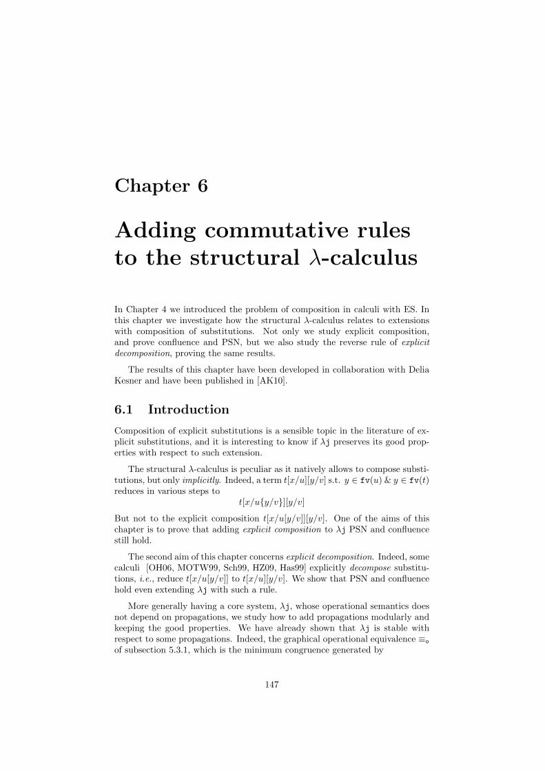
Chapter 6

Adding commutative rulesto the structural λ-calculus

In Chapter 4 we introduced the problem of composition in calculi with ES. Inthis chapter we investigate how the structural λ-calculus relates to extensionswith composition of substitutions. Not only we study explicit composition,and prove confluence and PSN, but we also study the reverse rule of explicitdecomposition, proving the same results.

The results of this chapter have been developed in collaboration with DeliaKesner and have been published in [AK10].

6.1 Introduction

Composition of explicit substitutions is a sensible topic in the literature of ex-plicit substitutions, and it is interesting to know if λj preserves its good prop-erties with respect to such extension.

The structural λ-calculus is peculiar as it natively allows to compose substi-tutions, but only implicitly. Indeed, a term t[x/u][y/v] s.t. y ∈ fv(u) & y ∈ fv(t)reduces in various steps to

t[x/uy/v][y/v]

But not to the explicit composition t[x/u[y/v]][y/v]. One of the aims of thischapter is to prove that adding explicit composition to λj PSN and confluencestill hold.

The second aim of this chapter concerns explicit decomposition. Indeed, somecalculi [OH06, MOTW99, Sch99, HZ09, Has99] explicitly decompose substitu-tions, i.e., reduce t[x/u[y/v]] to t[x/u][y/v]. We show that PSN and confluencehold even extending λj with such a rule.

More generally having a core system, λj, whose operational semantics doesnot depend on propagations, we study how to add propagations modularly andkeeping the good properties. We have already shown that λj is stable withrespect to some propagations. Indeed, the graphical operational equivalence ≡o

of subsection 5.3.1, which is the minimum congruence generated by

147

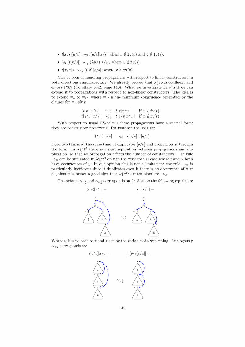
• t[x/s][y/v] ∼CS t[y/v][x/s] when x /∈ fv(v) and y /∈ fv(s).

• λy.(t[x/s]) ∼σ1 (λy.t)[x/s], where y /∈ fv(s).

• t[x/s] v ∼σ2(t v)[x/s], where x /∈ fv(v).

Can be seen as handling propagations with respect to linear constructors inboth directions simultaneously. We already proved that λj/o is confluent andenjoys PSN (Corollary 5.42, page 146). What we investigate here is if we canextend it to propagations with respect to non-linear constructors. The idea isto extend ≡o to ≡f0 , where ≡f0 is the minimum congruence generated by theclauses for ≡o plus:

(t v)[x/u] ∼σ03

t v[x/u] if x /∈ fv(t)

t[y/v][x/u] ∼σ04

t[y/v[x/u]] if x /∈ fv(t)

With respect to usual ES-calculi these propagations have a special form:they are constructor preserving. For instance the λx rule:

(t u)[y/v] →@ t[y/v] u[y/v]

Does two things at the same time, it duplicates [y/v] and propagates it throughthe term. In λj/f0 there is a neat separation between propagations and du-plication, so that no propagation affects the number of constructors. The rule→@ can be simulated in λj/f0 only in the very special case where t and u bothhave occurrences of y. In our opinion this is not a limitation: the rule →@ isparticularly inefficient since it duplicates even if there is no occurrence of y atall, thus it is rather a good sign that λj/f0 cannot simulate →@.

The axioms ∼σ03

and ∼σ04

corresponds on λj-dags to the following equalities:

(t v)[x/u] = t v[x/u] =

r

w

@

vt

x

u

j

∼σ03

r

w

@

vt

x

u

j

Where w has no path to x and x can be the variable of a weakening. Analogously∼σ4

corresponds to:

t[y/v][x/u] = t[y/v[x/u]] =

t

y

v

x

u

j

j

∼σ04

t

y

v

x

u

j

j

148

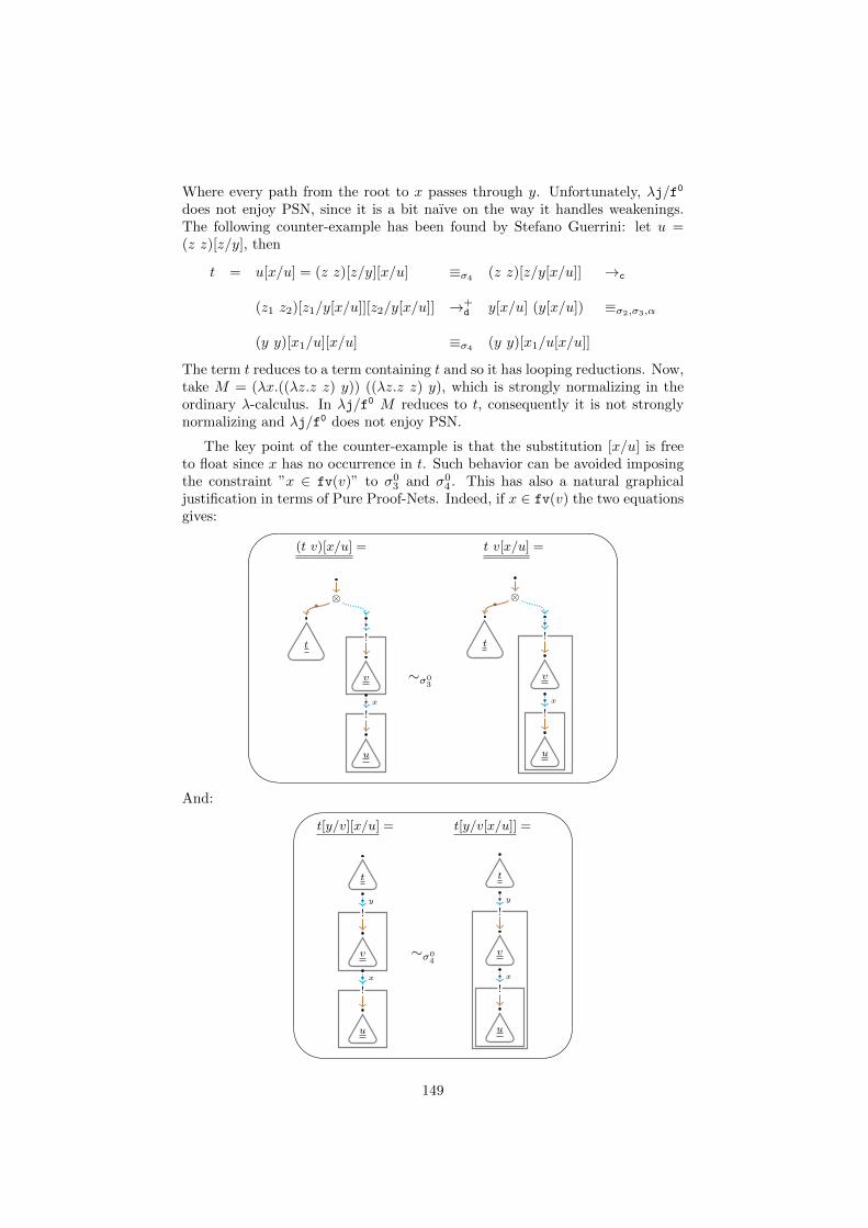
Where every path from the root to x passes through y. Unfortunately, λj/f0

does not enjoy PSN, since it is a bit naıve on the way it handles weakenings.The following counter-example has been found by Stefano Guerrini: let u =(z z)[z/y], then

t = u[x/u] = (z z)[z/y][x/u] ≡σ4(z z)[z/y[x/u]] →c

(z1 z2)[z1/y[x/u]][z2/y[x/u]] →+d y[x/u] (y[x/u]) ≡σ2,σ3,α

(y y)[x1/u][x/u] ≡σ4(y y)[x1/u[x/u]]

The term t reduces to a term containing t and so it has looping reductions. Now,take M = (λx.((λz.z z) y)) ((λz.z z) y), which is strongly normalizing in theordinary λ-calculus. In λj/f0 M reduces to t, consequently it is not stronglynormalizing and λj/f0 does not enjoy PSN.

The key point of the counter-example is that the substitution [x/u] is freeto float since x has no occurrence in t. Such behavior can be avoided imposingthe constraint ”x ∈ fv(v)” to σ0

3 and σ04 . This has also a natural graphical

justification in terms of Pure Proof-Nets. Indeed, if x ∈ fv(v) the two equationsgives: '

&

$

%

(t v)[x/u] = t v[x/u] =

⊗*

!*

v

x

!*

u

t

∼σ03

⊗*

!*

v

x

!*

u

t

And: '

&

$

%

t[y/v][x/u] = t[y/v[x/u]] =

t

y

!*

v

x

!*

u

∼σ04

t

y

!*

v

x

!*

u

149

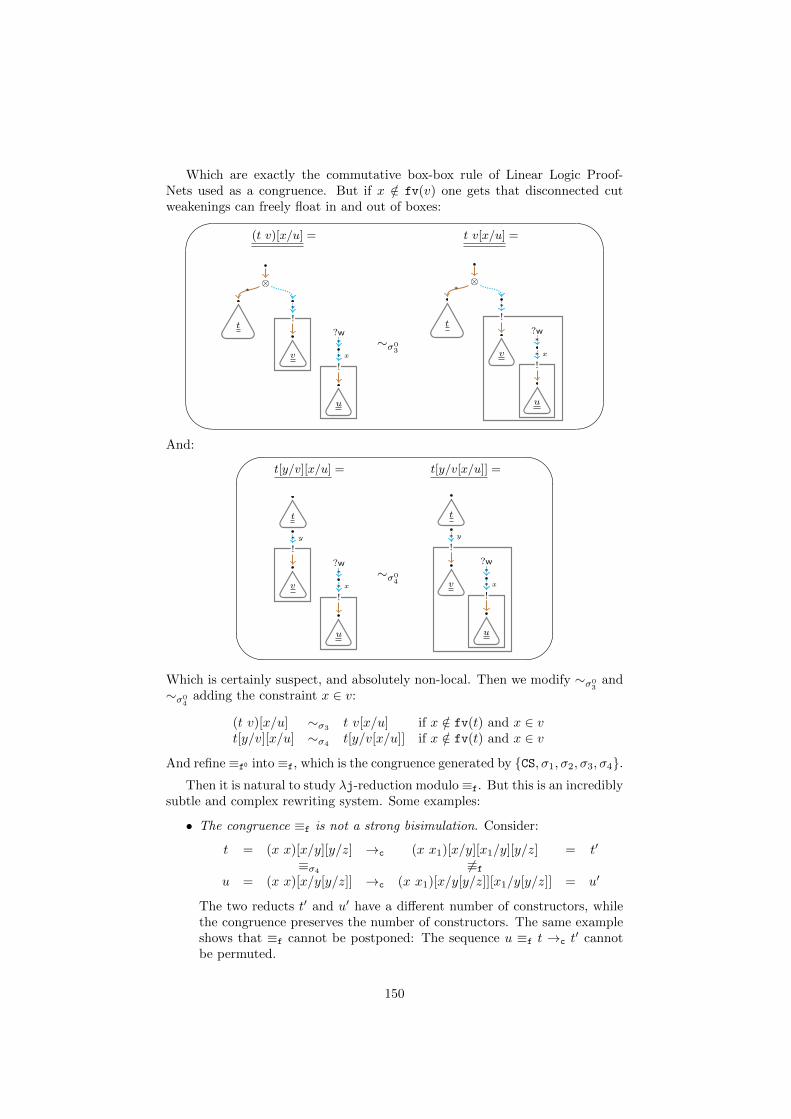
Which are exactly the commutative box-box rule of Linear Logic Proof-Nets used as a congruence. But if x /∈ fv(v) one gets that disconnected cutweakenings can freely float in and out of boxes:'

&

$

%

(t v)[x/u] = t v[x/u] =

⊗*

!*

v x

?w*

!*

u

t

∼σ03

⊗*

!*

v

t

x

?w*

!*

u

And: '

&

$

%

t[y/v][x/u] = t[y/v[x/u]] =

t

y

!*

v x

?w*

!*

u

∼σ04

t

y

!*

v x

?w*

!*

u

Which is certainly suspect, and absolutely non-local. Then we modify ∼σ03

and∼σ0

4adding the constraint x ∈ v:

(t v)[x/u] ∼σ3t v[x/u] if x /∈ fv(t) and x ∈ v

t[y/v][x/u] ∼σ4t[y/v[x/u]] if x /∈ fv(t) and x ∈ v

And refine ≡f0 into ≡f, which is the congruence generated by CS, σ1, σ2, σ3, σ4.Then it is natural to study λj-reduction modulo ≡f. But this is an incredibly

subtle and complex rewriting system. Some examples:

• The congruence ≡f is not a strong bisimulation. Consider:

t = (x x)[x/y][y/z] →c (x x1)[x/y][x1/y][y/z] = t′

≡σ46≡f

u = (x x)[x/y[y/z]] →c (x x1)[x/y[y/z]][x1/y[y/z]] = u′

The two reducts t′ and u′ have a different number of constructors, whilethe congruence preserves the number of constructors. The same exampleshows that ≡f cannot be postponed: The sequence u ≡f t →c t

′ cannotbe permuted.

150

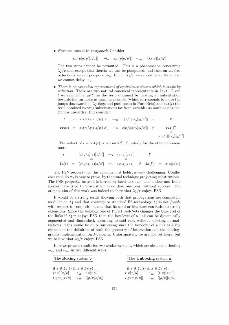
• Erasures cannot be postponed : Consider

λx.(y[y/y′[z/x]]) →w λx.(y[y/y′]) ∼σ1(λx.y)[y/y′]

The two steps cannot be permuted. This is a phenomenon concerningλj/o too, except that therein ≡o can be postponed, and then on ≡o-freereductions we can postpone →w. But in λj/f we cannot delay ≡f and sowe cannot delay →w.

• There is no canonical representant of equivalence classes which is stable byreduction. There are two natural canonical representants in λj/f. Givent we can define in(t) as the term obtained by moving all substitutiontowards the variables as much as possible (which corresponds to move thejumps downwards in λj-dags and pack boxes in Pure Nets) and out(t) theterm obtained moving substitutions far from variables as much as possible(jumps upwards). But consider:

t = x[x/(λy.z[z/y]) x′] →dB x[x/z[z/y][y/x′]] = t′

= =out(t) = x[x/(λy.z[z/y]) x′] →dB x[x/z[z/y][y/x′]] 6= out(t′)

=x[x/z][z/y][y/x′]

The reduct of t = out(t) is not out(t′). Similarly for the other represen-tant:

t = (x[y/z] z)[z/z′] →w (x z)[z/z′] = t′

= =in(t) = (x[y/z] z)[z/z′] →w (x z)[z/z′] 6= in(t′) = x z[z/z′]

The PSN property for this calculus, if it holds, is very challenging. Conflu-ence modulo ≡f is easy to prove, by the usual technique projecting substitutions.The PSN property, instead, is incredibly hard to tame. The author and DeliaKesner have tried to prove it for more than one year, without success. Theoriginal aim of this work was indeed to show that λj/f enjoys PSN.

It would be a strong result showing both that propagations are completelymodular on λj and that contrary to standard ES-technology λj is not fragilewith respect to composition, i.e., that its solid architecture can resist to strongextensions. Since the box-box rule of Pure Proof-Nets changes the box-level ofthe links if λj/f enjoys PSN then the box-level of a link can be dynamicallyaugmented and diminished, according to said rule, without affecting normal-izations. This would be quite surprising since the box-level of a link is a keyelement in the definition of both the geometry of interaction and the sharing-graphs implementation on λ-calculus. Unfortunately, we are not yet there, butwe believe that λj/f enjoys PSN.

Here we present results for two weaker systems, which are obtained orienting∼σ3 and ∼σ4 in two different ways:

The Boxing system b The Unboxing system u

if x /∈ fv(t) & x ∈ fv(v) : if x /∈ fv(t) & x ∈ fv(v) :(t v)[x/u] →ab t v[x/u] t v[x/u] →au (t v)[x/u]t[y/v][x/u] →sb t[y/v[x/u]] t[y/v[x/u]] →su t[y/v][x/u]

151

As we already pointed out these rules correspond to the commutative box-box rule of Linear Logic. The boxing system reflects exactly such rule, theunboxing system is obtained by using the reverse orientation. On terms tworules are needed, because there are two constructs which involve boxes, appli-cations and explicit substitutions. So a further aim of this work is the study ofthe commutative rule of Linear Logic, and the way it affects termination (andtermination proofs).

Switching from (un)boxing as a congruence to (un)boxing as a reduction weshall be able to prove PSN, but the “weaker” systems are still very subtle. Inparticular PSN for the unboxing system, of which we do not know any analogousresult in the literature, is more demanding than PSN for the boxing system (ofwhich there are instead many examples, see [Kes07]), and it brings a furtherstep of complexity in the proof, requiring to develop a non-trivial contextualreasoning.

In Chapter 7 we shall present an experimental graphical syntax which givesan interesting motivation to study propagations of substitutions.

6.1.1 Introducing the technique

We study the boxing and the unboxing system in a way as modular as possiblewith respect to the orientations of ∼σ3

and ∼σ4. From here on we use the letter

p to denote a parameter which represents any of the propagation systemsb, u. For every p ∈ b, u we consider its associated structural reductionsystem λjp, written λjb and λju respectively, defined by the reduction relationdB ∪ j ∪ p modulo the equivalence relation o, a relation which is denoted by→λjp .

Confluence can be proved using the same technique used for λj (Section4.2.3, page 102). So the following theorem holds:

Theorem 6.1 (Confluence Modulo). For all t1, t2 ∈ T , if t1 ≡o t2 andti →∗λjp ui (i = 1, 2), then ∃vi (i = 1, 2) s.t. ui →∗λjp vi (i = 1, 2) and v1 ≡o v2.

To prove PSN for λjb and λju it is sufficient, according to Theorem 4.25,to show the IE property. However, a simple inductive argument like the oneused for λj-reduction relation does no longer work (see the end of section 4.3).Therefore we shall show the IE property by adapting the technique in [Kes07].This has proven a challenging venture, and a very technically proof, despite thegeneral pattern of the proof is simple.

We have to prove that if u ∈ SN λjp and tx/uv1n ∈ SN λjp then t[x/u]v1

n ∈SN λjp . Informally, the proof proceeds as follows:

• We give a special status to [x/u], labeling it as [[x/u]]. This requires toextend the syntax and the rules of the system to labelled substitutions.

• The idea is that the label construct is used to trace reductions on residualsof [x/u].

• The labelled system is defined so that it splits into two quite independentsubsystem, one containing the reduction of and inside labelled substitu-tions and another containing reduction outside labelled substitutions.

152

• We show that under the hypothesis of IE the reduction of and insidelabelled substitutions is strongly normalizing (SN ).

• We show that this implies that t[[x/u]]v1n is SN .

• We show that anything that can be done in the standard system startingfrom t[x/u]v1

n can be lift to the labelled system, so that we get t[x/u]v1n ∈

SN λjp .

The technique is quite heavy because we have to pass through an auxiliarysystem, the labelled one. There are essentially three main steps:

Step 1: The proper definition of the labelled system.

Step 2: The proof that t[[x/u]]v1n is SN under the hypothesis of the IE

property.

Step 3: The simulation of λjp by its labelled variant.

The first step is easy but delicate, because we have to code into the labelledsystem the hypothesis we have on t[[x/u]]v1

n. The difficult step is the second. Itis not so difficult once the needed measures are known, of course the difficultyis in finding them. The third one is essentially an easy check that the definitionof the first step were well-chosen.

To ease the language an explicit substitution is often called a jump. Noambiguity arises, since in this chapter we shall not deal with λj-dags.

The proofs that we are going to present are complex and require manyintermediary lemmas. We omit most of the proofs of the easy lemmas, in orderto improve readability. The important lemmas are proved in the appendixes ofthe chapter.

6.2 Step 1: The Labeled Systems

Definition 6.2 (Labeled Terms). The set T of labeled terms is generatedusing the following grammar:

t ::= x | t t | λx.t | t[x/t] | t[[x/t]]

153

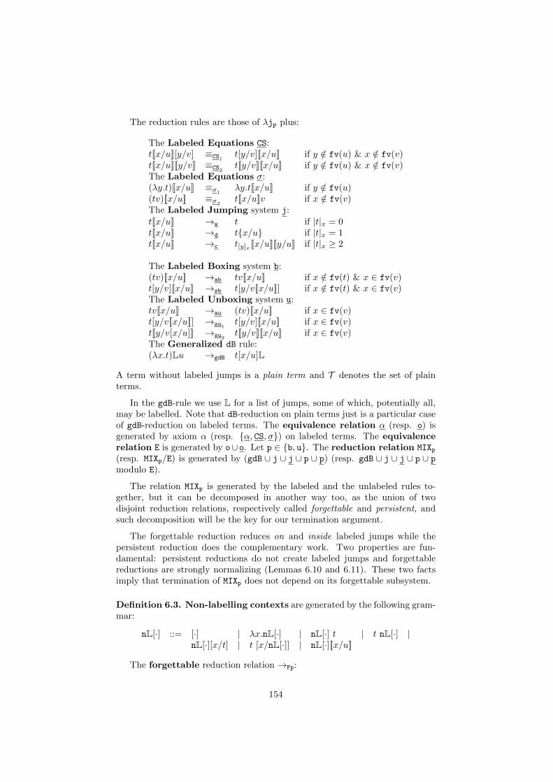
The reduction rules are those of λjp plus:

The Labeled Equations CS:t[[x/u]][y/v] ≡CS1

t[y/v][[x/u]] if y /∈ fv(u) & x /∈ fv(v)t[[x/u]][[y/v]] ≡CS2

t[[y/v]][[x/u]] if y /∈ fv(u) & x /∈ fv(v)The Labeled Equations σ:(λy.t)[[x/u]] ≡σ1

λy.t[[x/u]] if y /∈ fv(u)(tv)[[x/u]] ≡σ2

t[[x/u]]v if x /∈ fv(v)The Labeled Jumping system j:

t[[x/u]] →w t if |t|x = 0t[[x/u]] →d tx/u if |t|x = 1t[[x/u]] →c t[y]x [[x/u]][[y/u]] if |t|x ≥ 2

The Labeled Boxing system b:(tv)[[x/u]] →ab tv[[x/u]] if x /∈ fv(t) & x ∈ fv(v)t[y/v][[x/u]] →sb t[y/v[[x/u]]] if x /∈ fv(t) & x ∈ fv(v)The Labeled Unboxing system u:tv[[x/u]] →au (tv)[[x/u]] if x ∈ fv(v)t[y/v[[x/u]]] →su1

t[y/v][[x/u]] if x ∈ fv(v)t[[y/v[x/u]]] →su2

t[[y/v]][[x/u]] if x ∈ fv(v)The Generalized dB rule:(λx.t)Lu →gdB t[x/u]L

A term without labeled jumps is a plain term and T denotes the set of plainterms.

In the gdB-rule we use L for a list of jumps, some of which, potentially all,may be labelled. Note that dB-reduction on plain terms just is a particular caseof gdB-reduction on labeled terms. The equivalence relation α (resp. o) isgenerated by axiom α (resp. α, CS, σ) on labeled terms. The equivalencerelation E is generated by o∪o. Let p ∈ b, u. The reduction relation MIXp(resp. MIXp/E) is generated by (gdB ∪ j ∪ j ∪ p ∪ p) (resp. gdB ∪ j ∪ j ∪ p ∪ p

modulo E).

The relation MIXp is generated by the labeled and the unlabeled rules to-gether, but it can be decomposed in another way too, as the union of twodisjoint reduction relations, respectively called forgettable and persistent, andsuch decomposition will be the key for our termination argument.

The forgettable reduction reduces on and inside labeled jumps while thepersistent reduction does the complementary work. Two properties are fun-damental: persistent reductions do not create labeled jumps and forgettablereductions are strongly normalizing (Lemmas 6.10 and 6.11). These two factsimply that termination of MIXp does not depend on its forgettable subsystem.

Definition 6.3. Non-labelling contexts are generated by the following gram-mar:

nL[·] ::= [·] | λx.nL[·] | nL[·] t | t nL[·] |nL[·][x/t] | t [x/nL[·]] | nL[·][[x/u]]

The forgettable reduction relation →Fp:

154

Action on labeled jumps: If t→j,p t′, then t→Fp t

′.

Action inside labeled jump: If v →λjp v′, then u[[x/v]]→Fp u[[x/v′]].

Closure by non-labelling contexts: If t→Fp t′, then nL[t]→Fp nL[t′].

The reduction relation generated by the action inside labeled jumps andclosure by non-labelling contexts is called the internal forgettable reduction,and noted →[[Fp]]. The persistent reduction relation →Pp:

Root non-labeled action: If t 7→gdB,j,p t′ (where 7→ denotes root reduction),

then t→Pp t′.

Closure by non-labelling contexts: If t→Pp t′, then nL[t]→Pp nL[t′].

6.2.1 Well-Formed Labeled Terms

We defined a grammar for labeled terms, but we are not interested in whateverlabeled term. Labels have been introduced to study the term in the statementof the IE property and its residuals, and so we need to isolate the correspondinglabeled terms. The term of the statement is the plain term t[x/u]v1

n and thehypothesis of the IE property are that tx/uv1

n and u are strongly normalizingin the plain system. We shall consider M = t[[x/u]]v1

n, where in particular udoes not contain any label. So it is natural to consider the following subset oflabeled terms:

Definition 6.4 (constrained labeled term). A constrained (labeled) termt is a labeled term s.t.:

1. The interior u of a labeled substitution [[x/u]] is a term without labels.

2. u is strongly normalizing.

Unfortunately this is not enough, since constrained terms are not stable byreduction. Consider:

y[[y/x x]][x/λz.(z)z]

Which is a constrained term which reduces to

y[[y/(λz.(z)z) λz.(z)z]]

Which is not a constrained term. Similarly the term:

x[[x/y]][y/z[[z/v]]]

Reduces to:x[[x/z[[z/v]]]]

Which has a labeled jump inside a labeled jump. The idea of tracing down theresiduals of [x/u] using [[x/u]] makes sense only if on such residuals we can use thesame hypothesis that we have on [x/u], so we need the constraints to be stableby reduction. This can be done by defining a predicate of well-formednessWF(t) on constrained terms s.t. if WF(t) is true then whenever t→MIXp t

′ we getthat t′ is constrained and WF(t′) holds. In order to formalize such predicate weneed some definitions. Note that in our examples there is a labeled substitution

155

s.t. the free variable of its content are captured in the term. Hence the notionof free variable contained in a labeled jump is particularly important.

The set of labeled free variables of a constrained term t ∈ T is given by:

Lfv(x) := ∅Lfv(u v) := Lfv(u) ∪ Lfv(v)Lfv(λx.u) := Lfv(u) \ xLfv(u[x/v]) := (Lfv(u) \ x) ∪ Lfv(v)Lfv(u[[x/v]]) := (Lfv(u) \ x) ∪ fv(v)

Note that if u is a plain term then Lfv(u) = ∅. Also Lfv(t) ⊆ fv(t).

From now on any labeled term we shall consider will be a constrained labeledterm.

If we were considering the boxing system only it would not be difficult todefine WF(t). Consider the term M = t[[x/u]]v1

n we are interested in. All thefree variables of u are free variables of M , which assures that no substitutioncan act on u or any of its residuals, since no rule can create a substitutionbinding a variable of u, and thus the counter-example is ruled out. Thus wecould simply say that WF(t) is true if any subterm s[z/w], s[[z/w]] or λz.s of tverifies z /∈ Lfv(s). It is easy to see that for the boxing system if WF(t) holdsthen t→MIXb t

′ implies t′ constrained and WF(t′) holds.

But the unboxing system requires a more sophisticated predicate. The reasonis that the unboxing rule can create substitutions binding variables of u. Moreprecisely if u = u′[z/s], with x ∈ fv(u′), we get:

M = t[[x/u′[z/s]]]v1n →su2

t[[x/u′]][[z/s]]v1n = M ′

Which breaks our predicate. We can remove the requirement that any subterms[[z/w]] verifies z /∈ Lfv(s), but this would not be enough because wrong-formedlabeled terms can be created using labeled jumps only. Consider:

y[[y/x x]][[x/λz.(z)z]]

Which is well-formed but, as before, reduces to a non-well formed labeled term.Consider again M = t[[x/u′[z/s]]]v1

n. The intuition is that its reduct M ′ is well-formed because if the new configuration [[x/u′]][[z/s]] reduces to [[x/u′z/s]],modifying the content of [[x/u′]], we get u′z/s ∈ SN λjp by our hypothesisu = u′[z/s] ∈ SN λjp . Then the idea is to define that WFu(t) holds if it satisfiesthe two constraints on labeled jumps and moreover:

1. Non-labeled binders do not capture labeled free variables: any subterms[z/w] or λz.s in t verifies z /∈ Lfv(s).

2. SN-Stability with respect to labeled substitution from the context : whenevert = C[s[[z/w]]] then recursively substituting the labeled jumps in C[·] in wgets a strongly normalizing term.

The second requirement is complex because we have to consider chains of labeledsubstitutions, not necessarily on the same level. In order to properly formulatethe predicate we need to fix some notations.

156

Notation: we use τ, σ for (meta-level) substitutions, i.e., finite func-tions from variables to terms. We use tσ to denote the application of themeta-level substitution σ to the term t, and we use juxtaposition to denotecomposition of substitutions, so that if τ and σ are meta-level substitutions τσis the substitution given by x(τσ) := (xτ)σ.

Definition 6.5 (SNL(·, γ)). A labeled term t ∈ T is SN-labelled for a(n im-plicit) substitution γ iff SNL(t, γ) holds:

SNL(x, γ) := true

SNL(t u, γ) := SNL(t, γ) & SNL(u, γ)SNL(λx.t, γ) := SNL(t, γ)SNL(t[x/u], γ) := SNL(t, γ) & SNL(u, γ)SNL(t[[x/u]], γ) := SNL(t, x/uγ) & uγ ∈ SN λjp

Finally, we can set:

Definition 6.6 (b, u, p-well-formed terms). A (constrained) labeled term t is

• b-well-formed, written t ∈WFb, iff any subterm s[z/w], s[[z/w]] or λz.sin t verifies z /∈ Lfv(s)

• u-well-formed, written t ∈WFu, iff

1. Any subterm s[z/w] or λz.s in t verifies z /∈ Lfv(s).

2. SNL(t, ∅) holds.

• p-well-formed, written t ∈WFp, if t ∈WFb or t ∈WFu.

Thus for example t0 = (x x)[[x/y]][[y/z]] is not b-well-formed since y is not alabeled free variable of t0, whereas t0 is u-well-formed since z ∈ SN λju . Also,t1 = y[y/x][x/λz.z z] is b and u well-formed but t2 = y[[y/x x]][[x/λz.z z]] isnot. More precisely, x is a labeled free variable of y[[y/x x]] so that t2 is notb-well-formed, and SNL(t2, ∅) does not hold (since (λz.z z)(λz.z z) /∈ SN λju)hence t2 is not u-well-formed.

Now we need to show that well-formed terms are stable by reduction. Forthe boxing systems it is more or less immediate, since no free variable can becaptured during reduction. For the unboxing system, instead, we need to showthat SNL(t, γ) is stable by reduction. For, we need the following lemmas:

Lemma 6.7. Let t ∈WFp.

1. If t0 ≡E t1, then Lfv(t0) = Lfv(t1).2. If t0 →MIXp t1, then Lfv(t0) ⊇ Lfv(t1).

Proof. By induction on t.

We extend the definition of reduction to meta-level substitutions: we noteγ →λju γ

′ if x belongs to the domain of γ, γ(x) = t, t →∗λju t′ and γ′ is the

substitution everywhere equal to γ except for γ′(x) = u′.

Lemma 6.8 (SNL(t, γ) and substitutions). Let t ∈WFu.

1. If SNL(t, γ) and γ →∗λju γ′, then SNL(t, γ′).

157

2. If u ∈ T , then SNL(tx/u, γ) = SNL(t, x/uγ).

3. If |t|x ≥ 2. Then, SNL(t, x/uγ) = SNL(t[y]x , y/ux/uγ).

4. If u ∈ T and x /∈ Lfv(t), then SNL(t, x/uγ) = SNL(t, γ).

Proof. By induction on t.

Then we can prove that SNL is stable by reduction:

Proposition (Stability of SNL). Let t ∈ WFu and SNL(t, γ). If t ≡E t′ ort→MIXp t

′, then SNL(t′, γ).

Proof. By induction on the relations using Lemma 6.8. Details in the appendix(page 171).

Since free variables cannot be captured we get:

Corollary 6.9. Let t ∈WFp. If t ≡E t′ or t→MIXp t

′ then t′ ∈WFp.

6.3 Step 2: Labeled IE

The goal of this subsection is to show the following labeled IE property: ifu ∈ SN λjp and tx/uv1

n ∈ SN λjp then t[[x/u]]v1n ∈ SN λjp .

We assume the following two termination results, for which the predicate onwell-formedness of the previous section is fundamental:

Lemma 6.10 (→Fb/E is SN ). The relation →Fb/E is terminating on b well-formed labeled terms.

Lemma 6.11 (→Fu/E is SN ). The relation →Fu/E is terminating on u well-formed labeled terms.

The proofs of both Lemmas are in Appendix 1, page 162. We postponesuch proofs to improve readability and guide the reader through the technique,hiding some technical details. However, the proofs of the last two lemmas arenon-trivial and clearly the heart of the proof of the two PSN properties.

Consider the following projection function P( ) from labeled terms to terms,which also projects MIXp into the reduction λjp:

P(x) := xP(λx.t) := λx.P(t)P(t u) := P(t) P(u)P(t[x/u]) := P(t)[x/P(u)]P(t[[x/u]]) := P(t)x/u

Note that if u is a plain term then P(u) = u. The next lemma, together withthe termination of →Fp/E, is the reason for the names forgettable an persistent.Indeed, →Pp/E steps persist after P(·) projection, in the sense that t0 →Pp t1implies P(t0)→+

λjpP(t1). On the contrary,→Fp/E steps may not project, i.e., we

only get that t0 →Fp t1 implies P(t0) →∗λjp P(t1). But there cannot be infinite→Fp reductions and so these steps can safely be forgotten.

158

Lemma 6.12. Let t0 ∈ T. Then,

1. t0 ≡E t1 implies P(t0) ≡o P(t1).2. t0 →Fp t1 implies P(t0)→∗λjp P(t1).

3. t0 →Pp t1 implies P(t0)→+λjp

P(t1).

Proof. By induction on labeled terms. The case t0 →su2t1 uses Lemma 4.2.

Lemma 6.13. Let t ∈WFp. If P(t) ∈ SN λjp , then t ∈ SN MIXp/E.

Proof. Since→MIXp=→Fp ∪ →Pp we show that t ∈ SN Fp∪Pp/E by using Lemma 6.12and termination of the forgettable relations (Lemma 6.10 and Lemma 6.11).

Now let p ∈ b, u and consider t, u, v1n ∈ T s.t. u ∈ SN λjp . We immediately

get t[[x/u]]v1n ∈WFp. Using P(t[[x/u]]v1

n) = tx/uv1n we thus conclude:

Corollary 6.14 (labeled IE). Let t, u, v1n ∈ T . If u ∈ SN λjp & tx/uv1

n ∈SN λjp , then t[[x/u]]v1

n ∈ SN MIXp/E.

6.4 Step 3: Unlabelling

The last step of our proof is to show that t[[x/u]]v1n ∈ SN MIXp implies t[x/u]v1

n ∈SN λjp by relating labeled terms and reductions to unlabeled terms and re-ductions. To do that, let us introduce an unlabelling function on labeledterms:

U(x) := xU(t u) := U(t) U(u)U(λx.t) := λx.U(t)U(t[x/u]) := U(t)[x/U(u)]U(t[[x/u]]) := U(t)[x/u]

Remark that if u is a plain term then U(u) = u. Also, fv(t) = fv(U(t)) andU(tx/u) = U(t)x/U(u).

The next proposition is the key connection between the labeled system andthe plain one. It says that unlabelling and reducing in the plain system com-mutes, i.e., that it possible to first reduce in the labeled system and then removethe labels.

Proposition 6.15 (unlabeled steps lift). If t ∈ WFp and U(t) →λjp u, then∃ v ∈WFp s.t. t→MIXp/E v and U(v) = u.

Proof. By induction on →λjp and case analysis. The key point in this proof isthe fact that the following cases are not possible:

• t = u[[y/w[[x/v]]]] for any p.

• t = u[[y/w]][x/v] with x ∈ fv(w) for any p.

• t = u[[y/w]][[x/v]] with x ∈ fv(w) for p = b.

• t = u[[y/w]][[x/v]] with x /∈ fv(u) & x ∈ fv(w) and U(t)→sb t′1 for p = u.

Details are in the appendix, page 173.

159

The last lemma can be used to project an infinite reduction from U(t) in theplain system onto an infinite reduction from t in the labeled system. So we get:

Lemma 6.16 (unlabelling preserves SN). Let t ∈ WFp. If t ∈ SN MIXp/E, thenU(t) ∈ SN λjp .

Proof. We prove U(t) ∈ SN λjp by induction on ηMIXp/E(t). This is done byconsidering all the λjp-reducts of U(t) and using proposition 6.15.

Now let p ∈ b, u and consider t, u, v1n ∈ T s.t. u ∈ SN λjp . We immediately

get t[[x/u]]v1n ∈ WFp, since it has only one labeled jump [[x/u]] and no binder

captures its variables. By the labeled IE property we get t[[x/u]]v1n ∈ SN MIXp/E

and by the previous lemma we get t[x/u]v1n ∈ SN λjp . Hence we proved:

Lemma 6.17 (IE for λjp). For p ∈ b, u, λjp enjoys the IE property.

Theorem 4.25 thus allows us to conclude with the main result of this Chapter:

Corollary 6.18 (PSN for λjp). For p ∈ b, u, λjp enjoys PSN.

6.4.1 Some considerations on ≡o and (un)boxing

The proofs presented in this chapter can probably be re-organized my maskingthe use of congruences, if the (un)boxing rules are reformulated at a distance,so that ≡o becomes a strong bisimulation.

The crucial observation is that in our current formulation the congruence ≡o

is not a strong bisimulation. The problematic point is that it can create someredexes. Consider the following reduction modulo:

(x z)[x/y][z/y] ≡o (x z)[z/y][x/y]→ab (x z[z/y])[x/y]

The →b redex is created by the congruence step. Similarly for unboxing:

x z[z/y][z′/y] ≡o x z[z′/y][z/y]→au (x z[z′/y])[z/y]

Let us starting by reformulating ≡o. This is not strictly necessary, but ithelps to understand. Essentially, ≡o permits to freely move substitutions ina linear level, at the condition of respecting the binding of variables. We canexplicitate this through the notion of linear context.

Definition 6.19 (linear context). A linear context Lin[·] is defined by thefollowing grammar:

Lin[·] ::= [·] | λx.Lin[·] | Lin[·] t | Lin[·][x/t]

Now we can reformulate ≡o:

Definition 6.20 (≡′o). Let ≡′o be the smallest congruence on λj-terms contain-ing:

Lin[t[x/u]] ∼′o Lin[t][x/u] if |Lin[t]|x = |t|x and Lin[·]#u

Where we use Lin[·]#u to say that Lin[·] does not capture any free variable ofu.

160

Let us prove that they are equivalent

Lemma 6.21. t ≡o t′ iff t ≡′o t′.

Proof. ⇐) If M = Lin[t[x/u]] ∼′o Lin[t][x/u] = M ′ then by induction on Lin[·]one shows that M ∼nCS,σ1,σ2

M ′. So that the closure of ∼′o is contained in theclosure of ∼nCS,σ1,σ2

, which is ≡o. ⇒) M ∼CS,σ1,σ2M ′ clearly implies M ∼′o M ′,

which gives ≡o⊆≡′o.

If we re-consider our example of creation:

(x z)[x/y][z/y] ≡o (x z)[z/y][x/y]→b (x z[z/y])[x/y]

Now it is clear that if we allow the boxing rule to act modulo the linear contextLin[·] = [·][x/y] we get:

(x z)[x/y][z/y]→b (x z[z/y])[x/y]

And the redex which was created in the standard formulation now is visiblefrom the beginning. So we need to formulate the (un)boxing rules so that theyact modulo a linear context. Boxing becomes: if |Lin[t v]|x = |v|x > 0

Lin[t v][x/u] →ab′ Lin[t v[x/u]]Lin[t [y/v]][x/u] →sb′ Lin[t [y/v[x/u]]]

For unboxing analogously but simmetrically we get: if |t Lin[v]|x = |v|x > 0,|t [y/Lin[v]]|x = |v|x > 0 and Lin[·]#u

t Lin[v[x/u]] →au′ (t Lin[v])[x/u]t [y/Lin[v[x/u]]] →su′ t [y/Lin[v]][x/u]

Since we are working with contexts we can compact the two rules of each ori-entation by defining a level Lev[·] as

Lev[·] ::= t [·] | t[x/[·]]

Note that the two contexts on the right are base cases, so that this is not aninductive definition. Then we get:

Boxing:

Lin[Lev[v]][x/u] →b′ Lin[Lev[v[x/u]]] If |Lin[Lev[v]]|x = |v|x

Unboxing:

Lev[Lin[v[x/u]]] →u′ Lev[Lin[v][x/u] If |Lev[Lin[v]]|x = |v|xand Lev[Lin[·]]#u

Then one should prove:

Lemma 6.22. ≡o is a strong bisimulation with respect to →p′ , i.e., t ≡o→p′ t′

implies t→p′≡o t′.

We have not proved this lemma, since only towards the end of the redac-tion of the thesis we realized that an alternative formulation was possible andprobably useful. However, its statement is reasonable.

Let λj′p be the system generated by the rules dB, w, d, c and →′p. From thelast lemma the following sequence of corollaries should follow easily:

161

Corollary 6.23. ≡o is a strong bisimulation on λj′p.

By the properties of strong bisimulations (lemma 3.57, page 86) then itwould follow:

Corollary 6.24. t→∗λj′p/o t′ iff t→∗λj′p≡o t

′.

The following lemma is more or less evident (we did not prove it):

Corollary 6.25. t→λjp t′ iff t→λj′p/o

t′.

And from that we would get:

Corollary 6.26. λj′p/o enjoys PSN.

But the interest in having ≡o as a strong bisimulation with respect to boxingand unboxing is that it is possible to procede the other way around. The ideais that PSN for λj′p is easier and more elegant to prove, because ≡o can bepostponed and so we only have to deal with plain rewriting.

The proof of PSN for the (un)boxing systems is very delicate and complex,which is why we have left for future work the careful check that our intuition iscorrect. We presented it nonetheless, since it is an interesting interplay betweenthe themes of the thesis, and it is based on strong intuitions.

Moreover, the proof we presented would not sensibly simplify. Indeed, ≡o

does not really disappear: in the new system(s) it is simply masked, hardcodedinto the (un)boxing rules. The definition of the labeled system does not need la-beled congruences, and the statements of the lemmas are simplified, but modulominor details the proofs stay the same, since the cases of the unboxing rules be-come much longer because they need an induction on the linear context, whichamounts to the congruence cases in our proof. However, it may be that the newsystems, admitting better operational properties allow for different and simplerproofs, or for new intuitions.

6.5 Appendix 1: The Forgettable Systems Ter-minate

The termination proofs for→Fb and→Fu are not really parametric in p, nonethe-less they both make use of potential multiplicities, which are extended to la-beled jumps by adding the following case to the notion given in Subsection 4.2.1(page 97).

Mx(u[[y/v]]) := Mx(u) + max(1, My(u)) · Mx(v)

We first prove that the propagations p preserve potential multiplicities.

Lemma 6.27. Let t0 ∈ T. Then:

• t0 ≡o,o t1 implies Mw(t) = Mw(t′).• t0 →p t1 implies Mw(t) = Mw(t′).

162

Proof. There is a graphical argument: potential multiplicities correspond toskeletal paths in λj-dags (see subsection 4.2.2, page 101), while the (un)boxingrules modifies jumps from non-weakening variables, which are non-skeletal edges,so that potential multiplicities cannot change. However, we show two cases, theothers are similar:

• (t v)[[x/u]]→ab t v[[x/u]], with x /∈ fv(t) and x ∈ fv(v). We get:

Mw((t v)[[x/u]]) =Mw(t v) + max(1, Mx(t v)) · Mw(u) =Mw(t v) + max(1, Mx(v)) · Mw(u) =Mw(t) + Mw(v) + max(1, Mx(v)) · Mw(u) =Mw(t) + Mw(v[[x/u]]) = Mw(t v[[x/u]])

• t[[y/v[x/u]]] →su2t[[y/v]][[x/u]], where x ∈ fv(v). First, let us show that

max(1, My(t)) · Mx(v) = max(1, max(1, My(t)) · Mx(v)). If y ∈ fv(t) then bothexpression are equal to My(t) ·Mx(v), as x ∈ fv(v), otherwise are both equalto Mx(v). Then:

Mw(t[[y/v[x/u]]]) =Mw(t) + max(1, My(t)) · Mw(v[x/u]) =Mw(t) + max(1, My(t)) · (Mw(v) + max(1, Mx(v)) · Mw(u)) =Mw(t) + max(1, My(t)) · (Mw(v) + Mx(v) · Mw(u)) =Mw(t) + max(1, My(t)) · Mw(v) + max(1, My(t)) · Mx(v) · Mw(u) =Mw(t[[y/v]]) + max(1, My(t)) · Mx(v) · Mw(u) =Mw(t[[y/v]]) + max(1, max(1, My(t)) · Mx(v)) · Mw(u) =Mw(t[[y/v]]) + max(1, Mx(t) + max(1, My(t)) · Mx(v)) · Mw(u) =Mw(t[[y/v]]) + max(1, Mx(t[[y/v]])) · Mw(u) =Mw(t[[y/v]][[x/u]])

To relate potential multiplicities and reductions we need two lemmas. Thefirst is used for →c-steps and the second for →w,d-steps. Using easy calculationand inductions one shows:

Lemma 6.28. Let t ∈ T and u ∈ T . Then,

1. If |u|w = 0, then Mw(tx/u) = Mw(t).

2. If |t|x = 1, then Mw(tx/u) = Mw(t) + max(1, Mx(t)) · Mw(u).

3. If |t|x ≥ 2, w 6= x, y and x 6= y then

(a) Mw(t) = Mw(t[y]x)

(b) My(t) = Mx(t[x]y ) + My(t[x]y ).

4. t→j t′ implies Mw(t) ≥ Mw(t′)

And also:

Lemma 6.29. Let t ∈WFp s.t. w /∈ Lfv(t). If t→[[Fp]] t′, then Mw(t) = Mw(t′).

163

Proof. By induction on t→[[Fp]] t′.

Potential multiplicities can be altered only by w, w and gdB-steps. In thefirst two cases they can decrease, in the last one they can be both increased ordecreased. Consider t0 = (λy.x)z[z/w] →gdB x[y/z[z/w]] = t1. Then Mw(t0) =1, while Mw(t1) = 0. Instead for t2 = (λy.yy)z[z/w] →gdB yy[y/z[z/w]] = t3 weget Mw(t2) = 1 and Mw(t3) = 2.

6.5.1 Termination of →Fb

The forgettable system contains the j-rules, the b-rule and reduction insidelabeled substitutions.

Let us start by considering the j-rules. We reason on the plain version butwhat we say is valid for labeled substitutions, too. We know that multisets ofpotential multiplicities are a terminating measure for the j-rules (see section 4.2,page 96). But we need to consider boxing steps, too. Potential multiplicitiesare invariant for boxing steps, and since the boxing reduction alone is stronglynormalizing and it does not create j-redexes, we can forget the boxing, usingabstract theorem 6.36, which guarantees that a subsystem with such propertiescan be safely be forgetten without altering termination. So we get terminationof j ∪ b, or rather j ∪ b.

But to prove the termination of the forgettable boxing reductions we needto take into account also the content of labeled substitutions. This can easilybe done by combining multisets of multiplicities with the maximal length ofreductions for such terms, which are SN by hypothesis, thus taking multisetsof pairs.

We use 〈x, y〉 for the ordered pair of x and y, and n · 〈x, y〉 to denote thepair 〈x, n · y〉. The operation n · 〈x, y〉 is extended to multisets in the followingway: if M is a multiset of pairs of integers then n · M is the multiset [n ·〈x, y〉 | 〈x, y〉 ∈ M ]. Moreover, to improve readability, we write M t 〈x, y〉rather than M t [〈x, y〉].

The boxing measure of t ∈WFb, written dep(t), is given by:

dep(x) := ∅dep(tu) := dep(t) t dep(u)dep(λx.t) := dep(t)dep(t[x/u]) := dep(t) t max(1, Mx(t)) · dep(u)dep(t[[x/u]]) := dep(t) t 〈ηλjb(u), Mx(t)〉

Remark that for every non-labeled term u we have dep(u) = ∅. We needtwo preliminary and elementary lemmas.

Lemma 6.30. Let u ∈ T , t ∈WFb and x /∈ Lfv(t). Then dep(t) = dep(tx/u).

Proof. By induction on t using Lemma 6.28 to deal with the jump case.

Lemma 6.31. If |t|x ≥ 2, then dep(t) = dep(t[y]x).

Proof. By induction on t.

164

The next lemma gives the exact relation between the boxing measure, thereductions and the equivalences.

Lemma 6.32. Let t0 ∈WFb. Then:

1. If t0 ≡o,o t1 , then dep(t0) = dep(t1).2. If t0 →p t1 , then dep(t0) = dep(t1).

3. If t0 →j t1, then dep(t0) > dep(t1).

4. If t0 →[[Fp]] t1, then dep(t0) > dep(t1).

Proof. By induction on the relations. We only show the the interesting cases.

• t0 = (tv)[[x/u]]→au tv[[x/u]] = t1 with x /∈ fv(t) and x ∈ fv(v). Then

dep((tv)[[x/u]]) =dep(t) t dep(v) t 〈η(u), Mx(v)〉 =dep(tv[[x/u]])

• t0 = t[y/v][[x/u]] →Comp t[y/v[[x/u]]] = t1 with x /∈ fv(t) and x ∈ fv(v).Then

dep(t[y/v][[x/u]]) =dep(t) t max(1, My(t)) · dep(v) t 〈η(u), Mx(t[y/v])〉 =dep(t) t max(1, My(t)) · dep(v) t max(1, My(t)) · 〈η(u), Mx(v)〉 =dep(t) t max(1, My(t)) · (dep(v) t 〈η(u), Mx(v)〉) =dep(t) t max(1, My(t)) · dep(v[[x/u]]) =dep(t[y/v[[x/u]]])

• t0 = t[[x/u]]→w t = t1 with |t|x = 0. Then

dep(t[[x/u]]) =dep(t) t 〈η(u), Mx(t)〉 >dep(t)

• t0 = t[[x/u]]→d tx/u = t1 with |t|x = 1.

dep(t[[x/u]]) =dep(t) t 〈η(u), Mx(t)〉 >dep(t) =L. 6.30

dep(tx/u)

• t0 = t[[x/u]]→c t[y]x [[x/u]][[y/u]] = t1 with |t|x > 1.

dep(t[[x/u]]) =dep(t) t 〈η(u), Mx(t)〉 >L. 6.28

dep(t[y]x) t 〈η(u), Mx(t[y]x)〉 t 〈η(u), My(t[y]x)〉 =L. 6.31

dep(t[y]x [[x/u]][[y/u]])

• t0 = t[[x/u]]→[[Fp]] t[[x/u′]] = t1. We have dep(t0) = dep(t)t〈η(u), Mx(t)〉 >

dep(t) t 〈η(u′), Mx(t)〉.

165

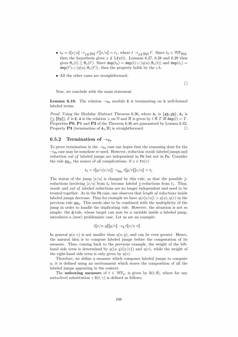
• t0 = t[[x/u]]→j,p,[[Fp]] t′[[x/u]] = t1, where t→j,p,[[Fp]] t

′. Since t0 ∈WF[[Fp]],

then the hypothesis gives x /∈ Lfv(t). Lemmas 6.27, 6.28 and 6.29 thengives Mx(t) ≥ Mx(t′). Since dep(t0) = dep(t) t 〈η(u), Mx(t)〉 and dep(t1) =dep(t′) t 〈η(u), Mx(t′)〉, then the property holds by the i.h.

• All the other cases are straightforward.

Now, we conclude with the main statement.

Lemma 6.10. The relation →Fb modulo E is terminating on b well-formedlabeled terms.

Proof. Using the Modular Abstract Theorem 6.36, where A1 is ab, sb, A2 isj, [[Fp]], E is E, A is the relation > on N and R is given by t R T iff dep(t) = T .Properties P0, P1 and P2 of the Theorem 6.36 are guaranteed by Lemma 6.32,Property P3 (termination of A1/E) is straightforward.

6.5.2 Termination of →Fu

To prove termination in the→Fu case one hopes that the reasoning done for the→Fb case may be somehow re-used. However, reduction inside labeled jumps andreduction out of labeled jumps are independent in Fb but not in Fu. Considerthe rule su2, the source of all complications: if x ∈ fv(v)

t0 = t[[y/v[x/u]]]→su2t[[y/v]][[x/u]] = t1

The status of the jump [x/u] is changed by this rule, so that the possible j-reductions involving [x/u] from t0 become labeled j-reductions from t1. Thus,inside and out of labeled reductions are no longer independent and need to betreated together. As in the Fb case, one observes that length of reductions insidelabeled jumps decrease. Thus for example we have η(v[x/u]) > η(u), η(v) in theprevious rule su2. This needs also to be combined with the multiplicity of thejump in order to handle the duplicating rule. However, the situation is not sosimple: the d-rule, whose target can now be a variable inside a labeled jump,introduces a (new) problematic case. Let us see an example:

t[[x/u y]][[y/v]]→d t[[x/u v]]

In general η(u v) is not smaller than η(u y), and can be even greater. Hence,the natural idea is to compose labeled jumps before the computation of itsmeasure. Thus, coming back to the previous example, the weight of the left-hand side term is determined by η((u y)x/v) and η(v), while the weight ofthe right-hand side term is only given by η(v).

Therefore, we define a measure which composes labeled jumps to computeη, it is defined using an environment which stores the composition of all thelabeled jumps appearing in the context.

The unboxing measure of t ∈ WFu, is given by D(t, ∅), where for anymeta-level substitution γ D(t, γ) is defined as follows:

166

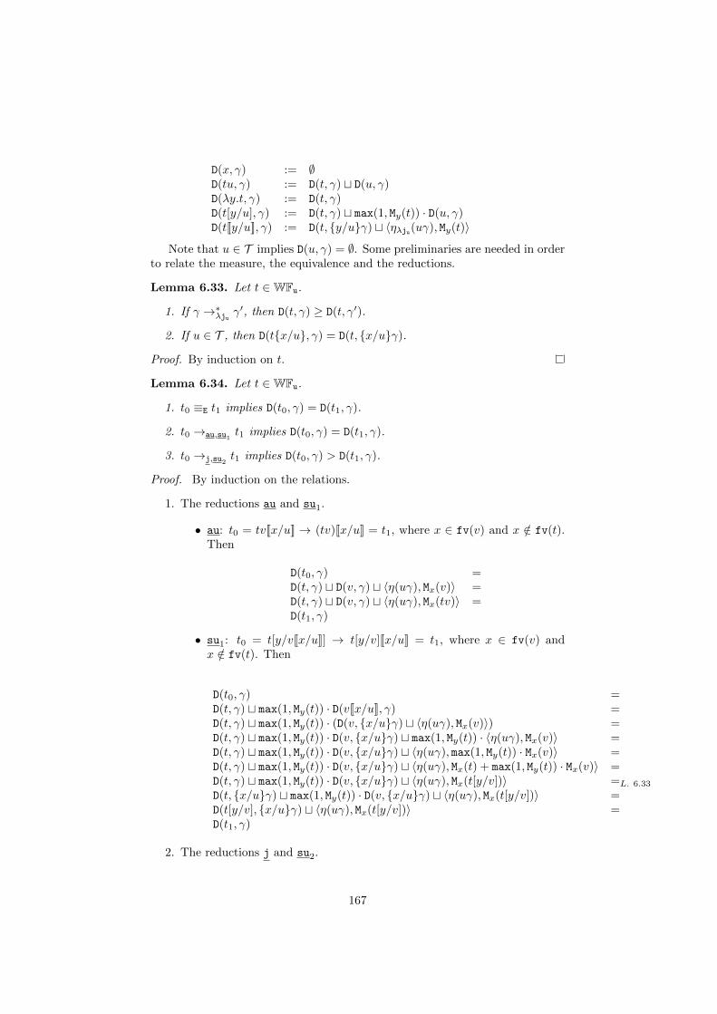
D(x, γ) := ∅D(tu, γ) := D(t, γ) t D(u, γ)D(λy.t, γ) := D(t, γ)D(t[y/u], γ) := D(t, γ) t max(1, My(t)) · D(u, γ)D(t[[y/u]], γ) := D(t, y/uγ) t 〈ηλju(uγ), My(t)〉

Note that u ∈ T implies D(u, γ) = ∅. Some preliminaries are needed in orderto relate the measure, the equivalence and the reductions.

Lemma 6.33. Let t ∈WFu.

1. If γ →∗λju γ′, then D(t, γ) ≥ D(t, γ′).

2. If u ∈ T , then D(tx/u, γ) = D(t, x/uγ).

Proof. By induction on t.

Lemma 6.34. Let t ∈WFu.

1. t0 ≡E t1 implies D(t0, γ) = D(t1, γ).

2. t0 →au,su1t1 implies D(t0, γ) = D(t1, γ).

3. t0 →j,su2t1 implies D(t0, γ) > D(t1, γ).

Proof. By induction on the relations.

1. The reductions au and su1.

• au: t0 = tv[[x/u]] → (tv)[[x/u]] = t1, where x ∈ fv(v) and x /∈ fv(t).Then

D(t0, γ) =D(t, γ) t D(v, γ) t 〈η(uγ), Mx(v)〉 =D(t, γ) t D(v, γ) t 〈η(uγ), Mx(tv)〉 =D(t1, γ)

• su1: t0 = t[y/v[[x/u]]] → t[y/v][[x/u]] = t1, where x ∈ fv(v) andx /∈ fv(t). Then

D(t0, γ) =D(t, γ) t max(1, My(t)) · D(v[[x/u]], γ) =D(t, γ) t max(1, My(t)) · (D(v, x/uγ) t 〈η(uγ), Mx(v)〉) =D(t, γ) t max(1, My(t)) · D(v, x/uγ) t max(1, My(t)) · 〈η(uγ), Mx(v)〉 =D(t, γ) t max(1, My(t)) · D(v, x/uγ) t 〈η(uγ), max(1, My(t)) · Mx(v)〉 =D(t, γ) t max(1, My(t)) · D(v, x/uγ) t 〈η(uγ), Mx(t) + max(1, My(t)) · Mx(v)〉 =D(t, γ) t max(1, My(t)) · D(v, x/uγ) t 〈η(uγ), Mx(t[y/v])〉 =L. 6.33

D(t, x/uγ) t max(1, My(t)) · D(v, x/uγ) t 〈η(uγ), Mx(t[y/v])〉 =D(t[y/v], x/uγ) t 〈η(uγ), Mx(t[y/v])〉 =D(t1, γ)

2. The reductions j and su2.

167

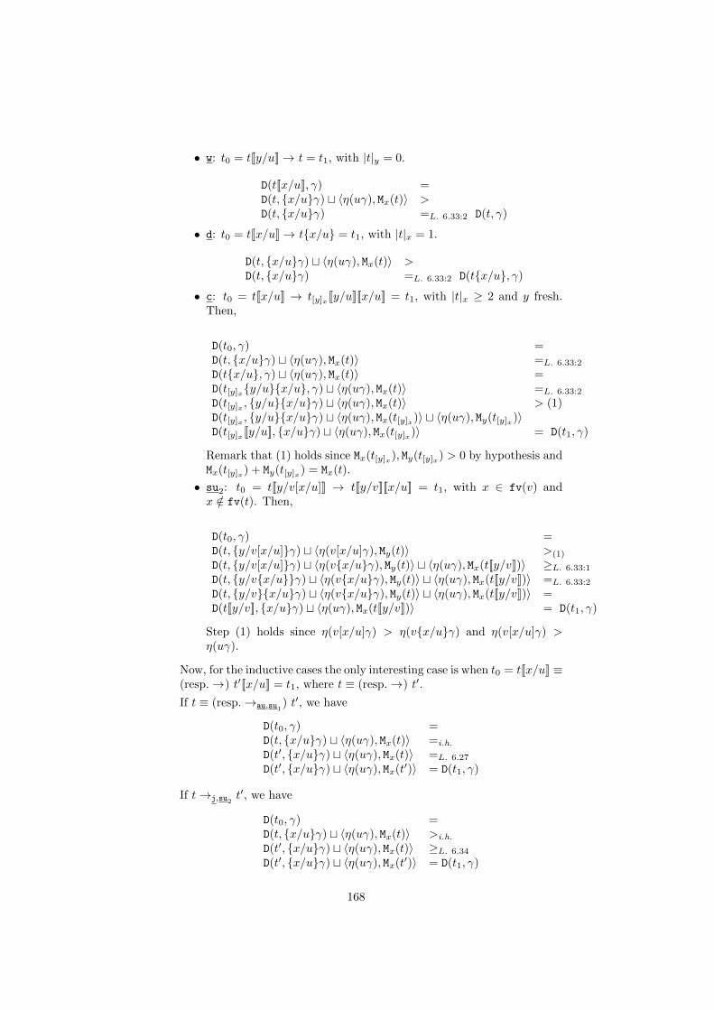
• w: t0 = t[[y/u]]→ t = t1, with |t|y = 0.

D(t[[x/u]], γ) =D(t, x/uγ) t 〈η(uγ), Mx(t)〉 >D(t, x/uγ) =L. 6.33:2 D(t, γ)

• d: t0 = t[[x/u]]→ tx/u = t1, with |t|x = 1.

D(t, x/uγ) t 〈η(uγ), Mx(t)〉 >D(t, x/uγ) =L. 6.33:2 D(tx/u, γ)

• c: t0 = t[[x/u]] → t[y]x [[y/u]][[x/u]] = t1, with |t|x ≥ 2 and y fresh.Then,

D(t0, γ) =D(t, x/uγ) t 〈η(uγ), Mx(t)〉 =L. 6.33:2

D(tx/u, γ) t 〈η(uγ), Mx(t)〉 =D(t[y]xy/ux/u, γ) t 〈η(uγ), Mx(t)〉 =L. 6.33:2

D(t[y]x , y/ux/uγ) t 〈η(uγ), Mx(t)〉 > (1)D(t[y]x , y/ux/uγ) t 〈η(uγ), Mx(t[y]x)〉 t 〈η(uγ), My(t[y]x)〉D(t[y]x [[y/u]], x/uγ) t 〈η(uγ), Mx(t[y]x)〉 = D(t1, γ)

Remark that (1) holds since Mx(t[y]x), My(t[y]x) > 0 by hypothesis andMx(t[y]x) + My(t[y]x) = Mx(t).

• su2: t0 = t[[y/v[x/u]]] → t[[y/v]][[x/u]] = t1, with x ∈ fv(v) andx /∈ fv(t). Then,

D(t0, γ) =D(t, y/v[x/u]γ) t 〈η(v[x/u]γ), My(t)〉 >(1)

D(t, y/v[x/u]γ) t 〈η(vx/uγ), My(t)〉 t 〈η(uγ), Mx(t[[y/v]])〉 ≥L. 6.33:1

D(t, y/vx/uγ) t 〈η(vx/uγ), My(t)〉 t 〈η(uγ), Mx(t[[y/v]])〉 =L. 6.33:2

D(t, y/vx/uγ) t 〈η(vx/uγ), My(t)〉 t 〈η(uγ), Mx(t[[y/v]])〉 =D(t[[y/v]], x/uγ) t 〈η(uγ), Mx(t[[y/v]])〉 = D(t1, γ)

Step (1) holds since η(v[x/u]γ) > η(vx/uγ) and η(v[x/u]γ) >η(uγ).

Now, for the inductive cases the only interesting case is when t0 = t[[x/u]] ≡(resp.→) t′[[x/u]] = t1, where t ≡ (resp.→) t′.

If t ≡ (resp.→au,su1) t′, we have

D(t0, γ) =D(t, x/uγ) t 〈η(uγ), Mx(t)〉 =i.h.

D(t′, x/uγ) t 〈η(uγ), Mx(t)〉 =L. 6.27

D(t′, x/uγ) t 〈η(uγ), Mx(t′)〉 = D(t1, γ)

If t→j,su2t′, we have

D(t0, γ) =D(t, x/uγ) t 〈η(uγ), Mx(t)〉 >i.h.

D(t′, x/uγ) t 〈η(uγ), Mx(t)〉 ≥L. 6.34

D(t′, x/uγ) t 〈η(uγ), Mx(t′)〉 = D(t1, γ)

168

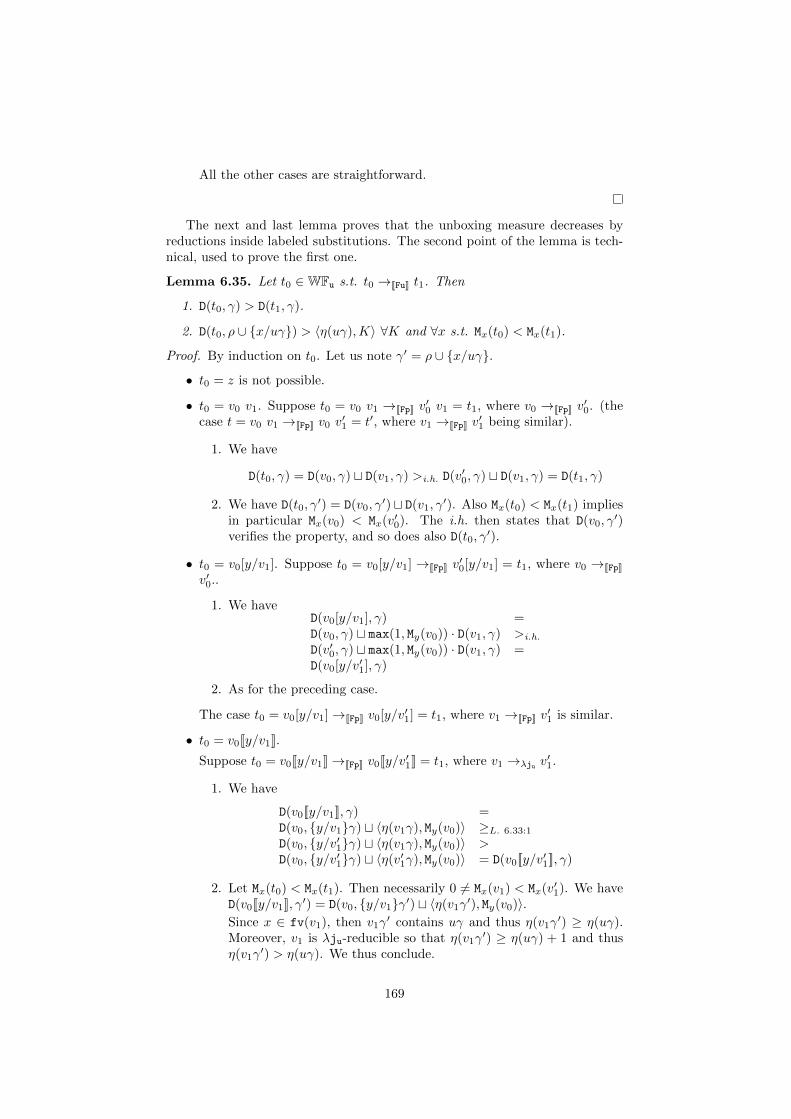
All the other cases are straightforward.

The next and last lemma proves that the unboxing measure decreases byreductions inside labeled substitutions. The second point of the lemma is tech-nical, used to prove the first one.

Lemma 6.35. Let t0 ∈WFu s.t. t0 →[[Fu]] t1. Then

1. D(t0, γ) > D(t1, γ).

2. D(t0, ρ ∪ x/uγ) > 〈η(uγ),K〉 ∀K and ∀x s.t. Mx(t0) < Mx(t1).

Proof. By induction on t0. Let us note γ′ = ρ ∪ x/uγ.

• t0 = z is not possible.

• t0 = v0 v1. Suppose t0 = v0 v1 →[[Fp]] v′0 v1 = t1, where v0 →[[Fp]] v

′0. (the

case t = v0 v1 →[[Fp]] v0 v′1 = t′, where v1 →[[Fp]] v

′1 being similar).

1. We have

D(t0, γ) = D(v0, γ) t D(v1, γ) >i.h. D(v′0, γ) t D(v1, γ) = D(t1, γ)

2. We have D(t0, γ′) = D(v0, γ

′) t D(v1, γ′). Also Mx(t0) < Mx(t1) implies

in particular Mx(v0) < Mx(v′0). The i.h. then states that D(v0, γ′)

verifies the property, and so does also D(t0, γ′).

• t0 = v0[y/v1]. Suppose t0 = v0[y/v1] →[[Fp]] v′0[y/v1] = t1, where v0 →[[Fp]]

v′0..

1. We haveD(v0[y/v1], γ) =D(v0, γ) t max(1, My(v0)) · D(v1, γ) >i.h.

D(v′0, γ) t max(1, My(v0)) · D(v1, γ) =D(v0[y/v′1], γ)

2. As for the preceding case.

The case t0 = v0[y/v1]→[[Fp]] v0[y/v′1] = t1, where v1 →[[Fp]] v′1 is similar.

• t0 = v0[[y/v1]].

Suppose t0 = v0[[y/v1]]→[[Fp]] v0[[y/v′1]] = t1, where v1 →λju v′1.

1. We have

D(v0[[y/v1]], γ) =D(v0, y/v1γ) t 〈η(v1γ), My(v0)〉 ≥L. 6.33:1

D(v0, y/v′1γ) t 〈η(v1γ), My(v0)〉 >D(v0, y/v′1γ) t 〈η(v′1γ), My(v0)〉 = D(v0[[y/v′1]], γ)

2. Let Mx(t0) < Mx(t1). Then necessarily 0 6= Mx(v1) < Mx(v′1). We haveD(v0[[y/v1]], γ′) = D(v0, y/v1γ′) t 〈η(v1γ

′), My(v0)〉.Since x ∈ fv(v1), then v1γ

′ contains uγ and thus η(v1γ′) ≥ η(uγ).

Moreover, v1 is λju-reducible so that η(v1γ′) ≥ η(uγ) + 1 and thus

η(v1γ′) > η(uγ). We thus conclude.

169

Suppose t0 = v0[[y/v1]]→[[Fp]] v′0[[y/v1]] = t1, where v0 →[[Fp]] v

′0.

1. We have D(v0[[y/v1]], γ) = D(v0, y/v1γ) t 〈η(v1γ), My(v0)〉 andD(v′0[[y/v1]], γ) = D(v′0, y/v1γ) t 〈η(v1γ), My(v′0)〉. Also,D(v0, y/v1γ) >i.h. (1) D(v′0, y/v1γ).

If My(v0) ≥ My(v′0), then 〈η(v1γ), My(v0)〉 ≥ 〈η(v1γ), My(v′0)〉 and weconclude.

If My(v0) < My(v′0), then D(v0, y/v1γ) >i.h. (2) 〈η(v1γ), My(v′0)〉 andwe also conclude.

• All the other cases are straightforward.

Lemma 6.11. The relation →Fu modulo E is terminating on u well-formedlabeled terms.

Proof. Using the Modular Abstract Theorem 6.36, where A1 is au, su1, A2 isj, su2, [[Fp]], E is E, A is the relation > on N and R is given by t R T iffD(t, ∅) = T . Properties P0, P1 and P2 of the Theorem 6.36 are guaranteed byLemmas 6.34 and 6.35, Property P3 (termination of A1/E) is straightforward.

6.6 Appendix 2: two lemmas and one theorem

The following theorem is used in most termination proofs of the chapter. It isformulated abstractly.

Theorem 6.36 (Modular Abstract Strong Normalisation). Let A1 and A2 (resp.E) be two reduction (resp. equivalence) relations on s. Let A be a reductionrelation on S and let consider a relation R ⊆ s× S. Suppose that forall u, v, U

(P0) u R U & u E v imply ∃V s.t. v R V & U = V .

(P1) u R U & u A1 v imply ∃V s.t. v R V & U A∗ V .

(P2) u R U & u A2 v imply ∃V s.t. v R V & U A+ V .

(P3) The relation A1 modulo E is well-founded.

Then, t R T & T ∈ SN A imply t ∈ SN (A1∪A2)/E .

Proof. Suppose t /∈ SN A1∪A2/E . Then, there is an infinite A1 ∪ A2/E reductionstarting at t, and since A1 modulo E is a well-founded relation by (P3), thisreduction has necessarily the form:

t →∗A1/E t1 →+A2/E t2 →∗A1/E t3 →+

A2/E t4 →∗A1/E . . .

And can be projected by (P0), (P1) and (P2) into an infinite A reductionsequence as follows:

t →∗A1/E t1 →+A2/E t2 →∗A1/E t3 →+

A2/E t4 →∗A1/E . . .

R R R R RT →∗A T1 →+

A T2 →∗A T3 →+A T4 →∗A . . .

But T ∈ SN A, absurd.

170

Then we show the proof of two of the lemmas in the chapter.

Proposition (6.2.1, page 158, Stability of SNL). Let t0 ∈WFu and SNL(t0, γ).If t0 ≡E t1 or t0 →MIXp t1, then SNL(t1, γ).

Proof. By induction on the reduction relations.

• d: t0 = t[y/u]→ ty/u = t1, where |t|y = 1.

Then, SNL(t0, γ) iff SNL(t, γ) and SNL(u, γ).

By Lemma 6.8 SNL(ty/u, γ) = SNL(t, y/uγ). But from t0 ∈ WFu weget that y /∈ Lfv(t) and by Lemma 6.8:4 we get SNL(t, y/uγ) = SNL(t, γ)which concludes this case.

• CS: t0 = t[x/u][y/v] ≡ t[y/v][x/u] = t1 if y /∈ fv(u) and x /∈ fv(v).

Then, SNL(t0, γ) iff SNL(t, γ) and SNL(u, γ) and SNL(v, γ) so that we con-clude SNL(t1, γ).

• CS1: t0 = t[[x/u]][y/v] ≡ t[y/v][[x/u]] = t1 if y /∈ fv(u) and x /∈ fv(v).

Then, SNL(t0, γ) iff SNL(t, x/uγ) and SNL(v, γ) and uγ ∈ SN λjp . Wealso haveSNL(v, γ) =L. 6.8:2 SNL(v, x/uγ). We thus conclude SNL(t1, γ).

• CS2: t0 = t[[x/u]][[y/v]] ≡ t[[y/v]][[x/u]] = t1 if y /∈ fv(u) and x /∈ fv(v).

Observe that the hypothesis implies uy/vγ = uγ and vx/uγ = vγ andx/uy/vγ = y/vx/uγ. Then, SNL(t0, γ) iff SNL(t, x/uy/vγ)and uγ, vγ ∈ SN λjp . Thus we conclude also SNL(t1, γ).

• σ1: t0 = (λy.t)[x/u] ≡ λy.t[x/u] = t1 if y /∈ fv(u).

Then, SNL(t0, γ) iff SNL(t, γ) and SNL(u, γ) so that SNL(t1, γ) is immedi-ate.

• σ1: t0 = (λy.t)[[x/u]] ≡ λy.t[[x/u]] = t1 if y /∈ fv(u).

Then, SNL(t0, γ) iff SNL(t, x/uγ) and uγ ∈ SN λjp so that SNL(t1, γ) isimmediate.

• σ2: t0 = (tv)[x/u] ≡ t[x/u]v = t1 if x /∈ fv(v) and x ∈ fv(t).

Then, SNL(t0, γ) iff SNL(t, γ) and SNL(v, γ) and SNL(u, γ) so that SNL(t1, γ)is immediate.

• σ2: t0 = t[[x/u]]v ≡ (tv)[[x/u]] = t1 if x /∈ fv(v).

Then, SNL(t0, γ) iff SNL(t, x/uγ) and SNL(v, x/uγ) and uγ ∈ SN λjp .We have SNL(v, x/uγ) =L. 6.8:2 SNL(v, γ) so that we conclude SNL(t1, γ).

• w: t0 = t[[y/u]]→ t = t1, where |t|y = 0.

Then, SNL(t0, γ) iff SNL(t, y/uγ) and uγ ∈ SN λjp .

By Lemma 6.8:2 SNL(t, γ) so that we conclude.

• d: t0 = t[[y/u]]→ ty/u = t1, where |t|y = 1.

Then, SNL(t0, γ) iff SNL(t, y/uγ) and uγ ∈ SN λjp .

By Lemma 6.8 SNL(ty/u, γ) which concludes this case.

171

• c: t0 = t[[x/u]]→ t[y]x [[y/u]][[x/u]] = t1, where |t|x ≥ 2 and y is fresh.

Then SNL(t0, γ) iff SNL(t, x/uγ) and uγ ∈ SN λjp .

On the other hand SNL(t1, γ) = SNL(t[y]x , y/ux/uγ) and uγ ∈ SN λjp .

Since SNL(t, x/uγ) =L 6.8:2 SNL(t[y]x , y/ux/uγ) then we conclude.

• ab: t0 = (tv)[[x/u]]→ tv[[x/u]] = t1, where x ∈ fv(v) and x /∈ fv(t).

Then, SNL(t0, γ) iff SNL(t, x/uγ) =L. 6.8:2 SNL(t, γ) and SNL(v, x/uγ)and uγ ∈ SN λjb . We thus conclude SNL(t1, γ).

• sb: t0 = t[y/v][[x/u]]→ t[y/v[[x/u]]] = t1, where x ∈ fv(v) and x /∈ fv(t).

Then, SNL(t0, γ) iff SNL(t, x/uγ) =L. 6.8:2 SNL(t, γ) and SNL(v, x/uγ)and uγ ∈ SN λju . We thus conclude SNL(t1, γ).

• au: t0 = tv[[x/u]]→ (tv)[[x/u]] = t1, where x ∈ fv(v) and x /∈ fv(t).

Then, SNL(t0, γ) iff SNL(t, γ) =L. 6.8:2 SNL(t, x/uγ) and SNL(v, x/uγ)and uγ ∈ SN λju . We thus conclude SNL(t1, γ).

• su1: t0 = t[y/v[[x/u]]]→ t[y/v][[x/u]] = t1, where x ∈ fv(v).

Then, SNL(t0, γ) iff SNL(t, γ) =L. 6.8:2 SNL(t, x/uγ) and SNL(v, x/uγ)and uγ ∈ SN λju . We thus conclude SNL(t1, γ).

• su2: t0 = t[[y/v[x/u]]]→ t[[y/v]][[x/u]] = t1, where x ∈ fv(v) and x /∈ fv(t).

Then, SNL(t0, γ) iff SNL(t, y/v[x/u]γ) and v[x/u]γ ∈ SN λju . To showSNL(t1, γ) we need uγ, vx/uγ ∈ SN λju and SNL(t, ρ), for ρ = y/vx/uγ.

Since uγ ∈ v[x/u]γ, then uγ ∈ SN λju . Since v[x/u]γ → vx/uγ, thenvx/uγ ∈ SN λju . Finally, y/v[x/u]γ →∗ y/vx/uγ = ρ′ so thatSNL(t, ρ′) holds by Lemma 6.8: 1. We conclude SNL(t1, γ).

• gdB: t0 = (λx.t)Lu→ t[x/u]L = t1. We can reason by induction on L.

If L is empty, then SNL(t0, γ) iff SNL(u, γ) and SNL(t, γ), which impliesSNL(t0, γ).

If L = [y/v], then it is straightforward. If L = [[y/v]], then SNL(t0, γ) iffSNL(u, γ) and SNL(t, y/vγ) and vγ ∈ SN λjp . Since y /∈ fv(u), thenLemma 6.8:2 gives SNL(u, y/vγ) so that we conclude SNL(t1, γ).

If L has more than one substitution, the proof is straightforward by thei.h.

• The inductive cases. We only show the interesting cases. Let t0 =t[[x/u]] ≡ t′[[x/u]] = t1 (resp. t0 = t[[x/u]] → t′[[x/u]] = t1). Then,SNL(t0, γ) iff SNL(t, x/uγ) and uγ ∈ SN λjp . The i.h. gives SNL(t′, x/uγ)so that SNL(t1, γ).

Let t0 = t[[x/u]] ≡ t[[x/u′]] = t1 or t0 = t[[x/u]] → t[[x/u′]] = t1. Then,SNL(t0, γ) iff SNL(t, x/uγ) and uγ ∈ SN λjp . We have uγ ≡ u′γ (resp.uγ →∗ u′γ) so that u′γ ∈ SN λjp . Lemma 6.8:1 gives SNL(t, x/u′γ) sothat we conclude SNL(t1, γ).

All the other cases are straightforward.

172

Proposition (6.15, page 159). If t ∈ WFp and U(t) →λjp u, then ∃ v ∈ WFp

s.t. t→MIXp/E v and U(v) = u.

Proof. By induction on →λjp and case analysis. We only show the interestingcases of root equivalence/reduction.

1. The congruence ≡o.

• t = u[x/v][[y/w]] with y /∈ fv(v) & x /∈ fv(w) and

U(u[x/v][[y/w]]) =U(u)[x/U(v)][y/w] ≡CS

U(u)[y/w][x/U(v)] = U(u[[y/w]][x/v]) = t′1

We then let t1 = u[[y/w]][x/v] so that U(t1) = t′1 and t ≡CS t1.

• t = u[[x/v]][y/w] with y /∈ fv(v) & x /∈ fv(w) and

U(u[[x/v]][y/w]) =U(u)[x/v][y/U(w)] ≡CS

U(u)[y/U(w)][x/v] = U(u[y/w][[x/v]]) = t′1

We then let t1 = u[y/w][[x/v]] so that U(t1) = t′1 and t ≡CS t1.

• t = u[[x/v]][[y/w]] with y /∈ fv(v) & x /∈ fv(w) and

U(u[[x/v]][[y/w]]) =U(u)[x/v][y/w] ≡CS

U(u)[y/w][x/v] = U(u[[y/w]][[x/v]]) = t′1

We then let t1 = u[[y/w]][[x/v]] so that U(t1) = t′1 and t ≡CS t1.

• t = λy.u[[x/v]] with y /∈ fv(v) and

U(λy.u[[x/v]]) =λy.U(u)[x/v] ≡SL

(λy.U(u))[x/v] = U((λy.u)[[x/v]]) = t′1

We then let t1 = (λy.u)[[x/v]] so that U(t1) = t′1 and t ≡SL t1.

• t = u[[x/v]]w and

U(u[[x/v]]w) =U(u)[x/v]U(w) ≡SAL

(U(u)U(w))[x/v] = U((uw)[[x/v]]) = t′1

We then let t1 = (uw)[[x/v]] so that U(t1) = t′1 and t ≡SALt1.

• All the other cases are straightforward.

2. The reduction relation →j.

• t = u[[x/v]] with |u|x = 0 and

U(u[[x/v]]) =U(u)[x/v] →w U(u) = t′1

We then let t1 = u so that U(t1) = t′1 and t→w t1.

173

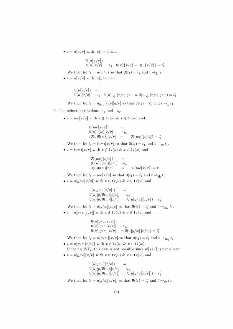
• t = u[[x/v]] with |u|x = 1 and

U(u[[x/v]]) =U(u)[x/v] →d U(u)x/v = U(ux/v) = t′1

We then let t1 = ux/v so that U(t1) = t′1 and t→d t1.

• t = u[[x/v]] with |u|x > 1 and

U(u[[x/v]]) =U(u)[x/v] →c U(u)[y]x [x/v][y/v] = U(u[y]x [x/v][y/v]) = t′1

We then let t1 = u[y]x [x/v][y/v] so that U(t1) = t′1 and t→c t1.

3. The reduction relations →b and →u.

• t = uw[[x/v]] with x /∈ fv(u) & x ∈ fv(w) and

U(uw[[x/v]]) =U(u)U(w)[x/v] →au

(U(u)U(w))[x/v] = U((uw)[[x/v]]) = t′1

We then let t1 = (uw)[[x/v]] so that U(t1) = t′1 and t→au t1.

• t = (uw)[[x/v]] with x /∈ fv(u) & x ∈ fv(w) and

U((uw)[[x/v]]) =(U(u)U(w))[x/v] →ab

U(u)U(w)[x/v] = U(uw[[x/v]]) = t′1

We then let t1 = uw[[x/v]] so that U(t1) = t′1 and t→ab t1.

• t = u[y/w[[x/v]]] with x /∈ fv(u) & x ∈ fv(w) and

U(u[y/w[[x/v]]]) =U(u)[y/U(w)[x/v]] →su

U(u)[y/U(w)][x/v] = U(u[y/w][[x/v]]) = t′1

We then let t1 = u[y/w][[x/v]] so that U(t1) = t′1 and t→su1t1.

• t = u[[y/w[x/v]]] with x /∈ fv(u) & x ∈ fv(w) and .

U(u[[y/w[x/v]]]) =U(u)[y/w[x/v]] →su

U(u)[y/w][x/v] = U(u[[y/w]][[x/v]]) = t′1

We then let t1 = u[[y/w]][[x/v]] so that U(t1) = t′1 and t→su2t1.

• t = u[[y/w[[x/v]]]] with x /∈ fv(u) & x ∈ fv(w).

Since t ∈WFp, this case is not possible since w[[x/v]] is not a term.

• t = u[y/w][[x/v]] with x /∈ fv(u) & x ∈ fv(w) and

U(u[y/w][[x/v]]) =U(u)[y/U(w)][x/v] →sb

U(u)[y/U(w)[x/v]] = U(u[y/w[[x/v]]]) = t′1

We then let t1 = u[y/w[[x/v]]] so that U(t1) = t′1 and t→sb t1.

174

• t = u[[y/w]][x/v] with x /∈ fv(u) & x ∈ fv(w). But t ∈WFp, so thatx /∈ Lfv(u[[y/w]]), which implies in particular x /∈ fv(w). This caseis not then possible.

• t = u[[y/w]][[x/v]] with x /∈ fv(u) & x ∈ fv(w). If t ∈ WFb, thenx /∈ fv(w) as before. This case is not then possible.

If t ∈WFu, then →sb does not hold in the u-system.

4. The reduction relation →gdB.

Consider t = (λx.u)Lv. Let L be the list containing all the unlabellingsubstitutions of the list L. Then,

U(t) =(λx.U(u))LU(v) →dB

U(u)[x/U(v)]L = U(u[x/v]L) = t′1

We then let t1 = u[x/v]L so that U(t1) = t′1 and t→gdB t1.

5. All the other cases are straightforward.

175

Chapter 7

An experiment

In this short chapter we ask ourself: is the way we use jumps minimal? Can weremove some jumps and still get a correctness criterion? We sketch an answerto these questions which can be seen as a motivation for the work in Chapter 6.

The necessary jumps are those on empty substitutions, which are thosesubstitutions with no occurrence, i.e., whose sharing node is the target of aweakening. The correctness criterion we used for λj-dags, in its dominationform (see Subsection 3.2.4, page 61), works. It simplifies, actually, as there isno longer need of asking domination for jumps.

In this framework for any given node u there may be many different correctsubnets rooted in u, so it is no longer clear how to define reductions. Weprove that from the point of view of correctness this is not a problem: anycorrect and connected subnet rooted in a substitution node can be used as abox, preserving correctness. Then we characterize the biggest subnet for a givennode, its empire, and give an example of empire reduction.

This material is experimental and requires further work. We decided toinclude it in this thesis because we think that it is quite intriguing. It hasbeen inspired by discussions with Stefano Guerrini but developed by the authoralone.

7.1 Static

Definition 7.1 (mλj-structure). A minimal λj-structureG, or mλj-structure,is a λj-structure satisfying the j-disjoint targets and the j-anchor conditionsplus the following minimal form of the j-source kind condition:

minimal j-sources kind: all and only the empty substitution nodes are targetsof jumps.

The translation ·X is refined to ·mX by changing the explicit substitutioncase as follows:

t [x/s]m

=

(tm ; 〈w|x〉) (sm † x) ; 〈ut|j|x〉 if x /∈ fv(s)

tm (sm † x) if x ∈ fv(s)

176

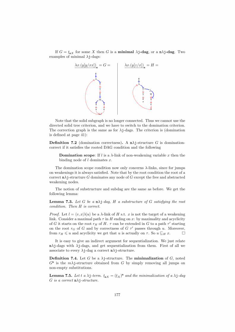
If G = tmX for some X then G is a minimal λj-dag, or a mλj-dag. Twoexamples of minimal λj-dags:

λx.(y[y/xx])m

= G = λx.(y[z/x])m

= H =

v

@

vv

λ

y

v w

v

λ

j

Note that the solid subgraph is no longer connected. Thus we cannot use thedirected solid tree criterion, and we have to switch to the domination criterion.The correction graph is the same as for λj-dags. The criterion is (dominationis defined at page 41):

Definition 7.2 (domination correctness). A mλj-structure G is domination-correct if it satisfies the rooted DAG condition and the following

Domination scope: If l is a λ-link of non-weakening variable x then thebinding node of l dominates x.

The domination scope condition now only concerns λ-links, since for jumpson weakenings it is always satisfied. Note that by the root condition the root of acorrect mλj-structure G dominates any node of G except the free and abstractedweakening nodes.

The notion of substructure and subdag are the same as before. We get thefollowing lemma:

Lemma 7.3. Let G be a mλj-dag, H a substructure of G satisfying the rootcondition. Then H is correct.

Proof. Let l = 〈v, x|λ|u〉 be a λ-link of H s.t. x is not the target of a weakeninglink. Consider a maximal path τ in H ending on x: by maximality and acyclicityof G it starts on the root rH of H. τ can be extended in G to a path τ ′ startingon the root rG of G and by correctness of G τ ′ passes through u. Moreover,from rH 6 u and acyclicity we get that u is actually on τ . So u vH x.

It is easy to give an indirect argument for sequentialization. We just relatemλj-dags with λj-dags, and get sequentialization from them. First of all weassociate to every λj-dag a correct mλj-structure.

Definition 7.4. Let G be a λj-structure. The minimalization of G, notedGm is the mλj-structure obtained from G by simply removing all jumps onnon-empty substitutions.

Lemma 7.5. Let t a λj-term. tmX = (tX)m and the minimalization of a λj-dagG is a correct mλj-structure.

177

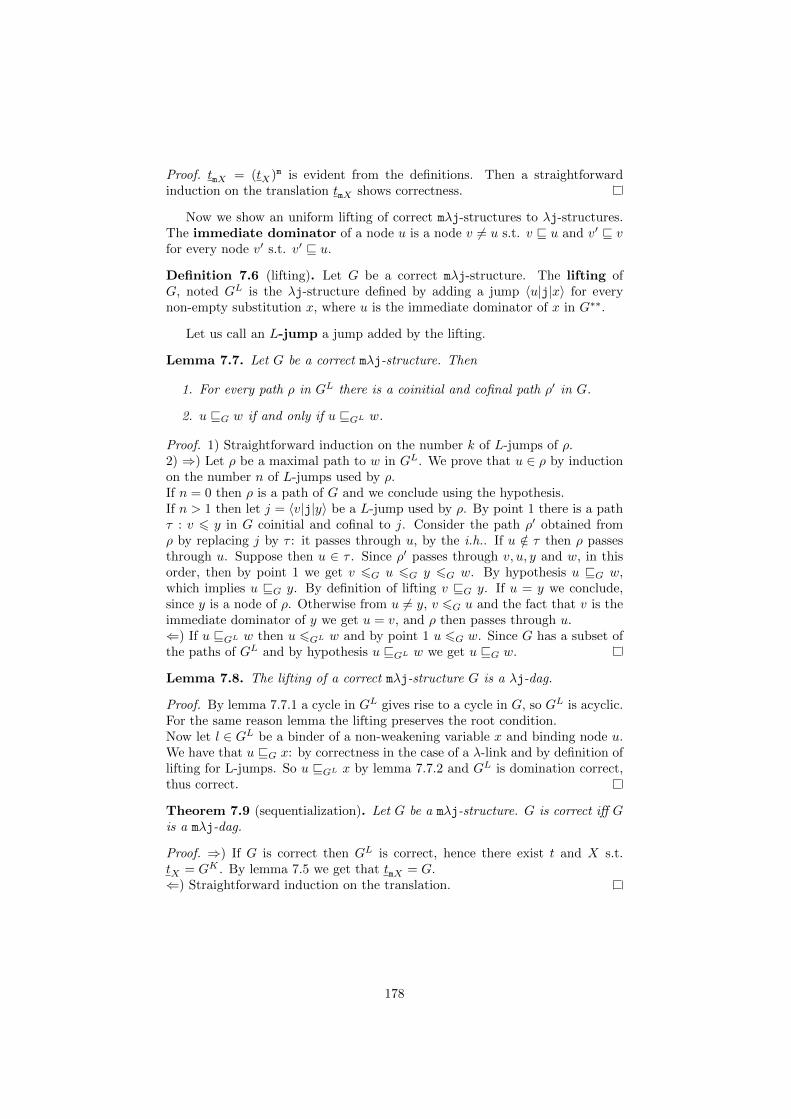
Proof. tmX = (tX)m is evident from the definitions. Then a straightforwardinduction on the translation tmX shows correctness.

Now we show an uniform lifting of correct mλj-structures to λj-structures.The immediate dominator of a node u is a node v 6= u s.t. v v u and v′ v vfor every node v′ s.t. v′ v u.

Definition 7.6 (lifting). Let G be a correct mλj-structure. The lifting ofG, noted GL is the λj-structure defined by adding a jump 〈u|j|x〉 for everynon-empty substitution x, where u is the immediate dominator of x in G∗∗.

Let us call an L-jump a jump added by the lifting.

Lemma 7.7. Let G be a correct mλj-structure. Then

1. For every path ρ in GL there is a coinitial and cofinal path ρ′ in G.

2. u vG w if and only if u vGL w.

Proof. 1) Straightforward induction on the number k of L-jumps of ρ.2) ⇒) Let ρ be a maximal path to w in GL. We prove that u ∈ ρ by inductionon the number n of L-jumps used by ρ.If n = 0 then ρ is a path of G and we conclude using the hypothesis.If n > 1 then let j = 〈v|j|y〉 be a L-jump used by ρ. By point 1 there is a pathτ : v 6 y in G coinitial and cofinal to j. Consider the path ρ′ obtained fromρ by replacing j by τ : it passes through u, by the i.h.. If u /∈ τ then ρ passesthrough u. Suppose then u ∈ τ . Since ρ′ passes through v, u, y and w, in thisorder, then by point 1 we get v 6G u 6G y 6G w. By hypothesis u vG w,which implies u vG y. By definition of lifting v vG y. If u = y we conclude,since y is a node of ρ. Otherwise from u 6= y, v 6G u and the fact that v is theimmediate dominator of y we get u = v, and ρ then passes through u.⇐) If u vGL w then u 6GL w and by point 1 u 6G w. Since G has a subset ofthe paths of GL and by hypothesis u vGL w we get u vG w.

Lemma 7.8. The lifting of a correct mλj-structure G is a λj-dag.

Proof. By lemma 7.7.1 a cycle in GL gives rise to a cycle in G, so GL is acyclic.For the same reason lemma the lifting preserves the root condition.Now let l ∈ GL be a binder of a non-weakening variable x and binding node u.We have that u vG x: by correctness in the case of a λ-link and by definition oflifting for L-jumps. So u vGL x by lemma 7.7.2 and GL is domination correct,thus correct.

Theorem 7.9 (sequentialization). Let G be a mλj-structure. G is correct iff Gis a mλj-dag.

Proof. ⇒) If G is correct then GL is correct, hence there exist t and X s.t.tX = GK . By lemma 7.5 we get that tmX = G.⇐) Straightforward induction on the translation.

178

'

&

$

%

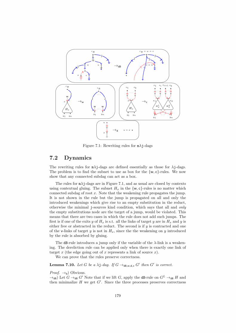
rR

j

w u

@

vx

λ

j →dB

rR = w = v

j

x = u

j j

'

&

$

%

rR

x

w

Hx

y1 yn

. . .

j

→w

rR

. . .

y1 yn

w w. . .

j j

'

&

$

%

o1 ok

. . .

x

v v

Hx

y1 yn

. . .

→c

o1 oi oi+1 ok

. . . . . .

x1

v v

x2

v v

H1x H2

x

y1 yn

. . .

u

x

v →d u = x

Figure 7.1: Rewriting rules for mλj-dags

7.2 Dynamics

The rewriting rules for mλj-dags are defined essentially as those for λj-dags.The problem is to find the subnet to use as box for the w, c-rules. We nowshow that any connected subdag can act as a box.

The rules for mλj-dags are in Figure 7.1, and as usual are closed by contextsusing contextual gluing. The subnet Hx in the w, c-rules is no matter whichconnected subdag of root x. Note that the weakening rule propagates the jump.It is not shown in the rule but the jump is propagated on all and only theintroduced weakenings which give rise to an empty substitution in the reduct,otherwise the minimal j-sources kind condition, which says that all and onlythe empty substitutions node are the target of a jump, would be violated. Thismeans that there are two cases in which the rule does not add such jumps. Thefirst is if one of the exits y of Hx is s.t. all the links of target y are in Hx and y iseither free or abstracted in the reduct. The second is if y is contracted and oneof the v-links of target y is not in Hx, since the the weakening on y introducedby the rule is absorbed by gluing.

The dB-rule introduces a jump only if the variable of the λ-link is a weaken-ing. The dereliction rule can be applied only when there is exactly one link oftarget x (the edge going out of x represents a link of source x).

We can prove that the rules preserve correctness.

Lemma 7.10. Let G be a λj-dag. If G→dB,w,d,c G′ then G′ is correct.

Proof. →d) Obvious.→dB) Let G→dB G

′ Note that if we lift G, apply the dB-rule on GL →dB H andthen minimalize H we get G′. Since the three processes preserves correctness

179

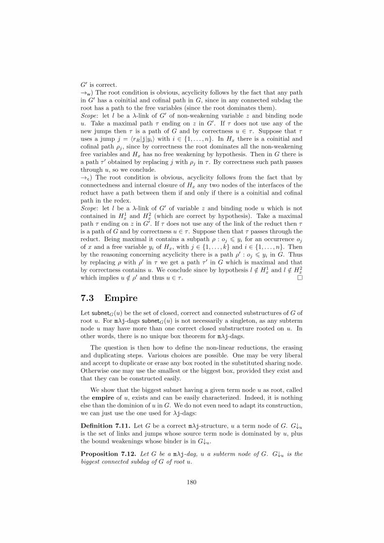
G′ is correct.→w) The root condition is obvious, acyclicity follows by the fact that any pathin G′ has a coinitial and cofinal path in G, since in any connected subdag theroot has a path to the free variables (since the root dominates them).Scope: let l be a λ-link of G′ of non-weakening variable z and binding nodeu. Take a maximal path τ ending on z in G′. If τ does not use any of thenew jumps then τ is a path of G and by correctness u ∈ τ . Suppose that τuses a jump j = 〈rR|j|yi〉 with i ∈ 1, . . . , n. In Hx there is a coinitial andcofinal path ρj , since by correctness the root dominates all the non-weakeningfree variables and Hx has no free weakening by hypothesis. Then in G there isa path τ ′ obtained by replacing j with ρj in τ . By correctness such path passesthrough u, so we conclude.→c) The root condition is obvious, acyclicity follows from the fact that byconnectedness and internal closure of Hx any two nodes of the interfaces of thereduct have a path between them if and only if there is a coinitial and cofinalpath in the redex.Scope: let l be a λ-link of G′ of variable z and binding node u which is notcontained in H1

x and H2x (which are correct by hypothesis). Take a maximal

path τ ending on z in G′. If τ does not use any of the link of the reduct then τis a path of G and by correctness u ∈ τ . Suppose then that τ passes through thereduct. Being maximal it contains a subpath ρ : oj 6 yi for an occurrence ojof x and a free variable yi of Hx, with j ∈ 1, . . . , k and i ∈ 1, . . . , n. Thenby the reasoning concerning acyclicity there is a path ρ′ : oj 6 yi in G. Thusby replacing ρ with ρ′ in τ we get a path τ ′ in G which is maximal and thatby correctness contains u. We conclude since by hypothesis l /∈ H1

x and l /∈ H2x

which implies u /∈ ρ′ and thus u ∈ τ .

7.3 Empire

Let subnetG(u) be the set of closed, correct and connected substructures of G ofroot u. For mλj-dags subnetG(u) is not necessarily a singleton, as any subtermnode u may have more than one correct closed substructure rooted on u. Inother words, there is no unique box theorem for mλj-dags.

The question is then how to define the non-linear reductions, the erasingand duplicating steps. Various choices are possible. One may be very liberaland accept to duplicate or erase any box rooted in the substituted sharing node.Otherwise one may use the smallest or the biggest box, provided they exist andthat they can be constructed easily.

We show that the biggest subnet having a given term node u as root, calledthe empire of u, exists and can be easily characterized. Indeed, it is nothingelse than the dominion of u in G. We do not even need to adapt its construction,we can just use the one used for λj-dags:

Definition 7.11. Let G be a correct mλj-structure, u a term node of G. G↓uis the set of links and jumps whose source term node is dominated by u, plusthe bound weakenings whose binder is in G↓u.

Proposition 7.12. Let G be a mλj-dag, u a subterm node of G. G↓u is thebiggest connected subdag of G of root u.

180

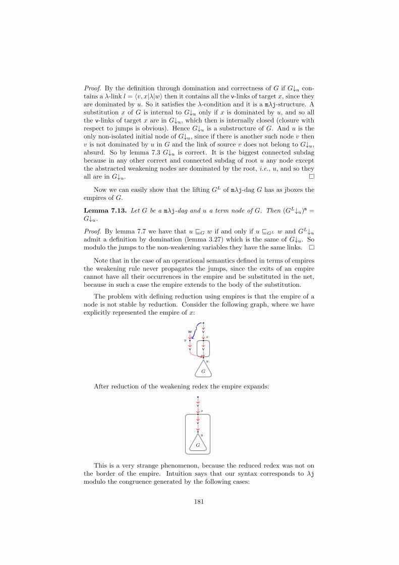
Proof. By the definition through domination and correctness of G if G↓u con-tains a λ-link l = 〈v, x|λ|w〉 then it contains all the v-links of target x, since theyare dominated by u. So it satisfies the λ-condition and it is a mλj-structure. Asubstitution x of G is internal to G↓u only if x is dominated by u, and so allthe v-links of target x are in G↓u, which then is internally closed (closure withrespect to jumps is obvious). Hence G↓u is a substructure of G. And u is theonly non-isolated initial node of G↓u, since if there is another such node v thenv is not dominated by u in G and the link of source v does not belong to G↓u,absurd. So by lemma 7.3 G↓u is correct. It is the biggest connected subdagbecause in any other correct and connected subdag of root u any node exceptthe abstracted weakening nodes are dominated by the root, i.e., u, and so theyall are in G↓u.

Now we can easily show that the lifting GL of mλj-dag G has as jboxes theempires of G.

Lemma 7.13. Let G be a mλj-dag and u a term node of G. Then (GL↓u)m =G↓u.

Proof. By lemma 7.7 we have that u vG w if and only if u vGL w and GL↓uadmit a definition by domination (lemma 3.27) which is the same of G↓u. Somodulo the jumps to the non-weakening variables they have the same links.

Note that in the case of an operational semantics defined in terms of empiresthe weakening rule never propagates the jumps, since the exits of an empirecannot have all their occurrences in the empire and be substituted in the net,because in such a case the empire extends to the body of the substitution.

The problem with defining reduction using empires is that the empire of anode is not stable by reduction. Consider the following graph, where we haveexplicitly represented the empire of x:

x

v

y

v

y

wj

v

G

After reduction of the weakening redex the empire expands:

x

v

y

v

G

This is a very strange phenomenon, because the reduced redex was not onthe border of the empire. Intuition says that our syntax corresponds to λjmodulo the congruence generated by the following cases:

181

t[x/u][y/v] ∼CS t[y/v][x/u] if x /∈ fv(v) and y /∈ fv(u)(λy.t)[x/u] ∼′σ1

λy.(t[x/u]) if x ∈ fv(t) and y /∈ fv(u)(t v)[x/u] ∼′σ2

t[x/u] v if x ∈ fv(t) and x /∈ fv(v)(t v)[x/u] ∼σ3

t v[x/u] if x /∈ fv(t) and x ∈ vt[y/v][x/u] ∼σ4

t[y/v[x/u]] if x /∈ fv(t) and x ∈ v

Which is not exactly λj/f because empty substitutions cannot move in ∼′σ1

and ∼′σ2, which corresponds to the fact that there are jumps on substituted

weakenings.

In this syntax the empire reduction can be seen to correspond to the followingvery special strategy to reduce a substitution [y/u] in a term t:

1. First consider the term in(t) obtained from t by taking the normal formwith respect to the orientation from left to right of ∼′σ1

, ∼′σ2, ∼σ3

and∼σ4 , which is unique modulo ≡CS;

2. Then reduce [y/u′] in in(t).

Let us reconsider our graphical example in a sequential form. It can beseen as the term t = x[x/y][z/y][y/v], where the term v corresponds to G,which is s.t. in(t) = t. The reduction we have considered corresponds to:t = x[x/y][z/y][y/v] →w x[x/y][y/v] = t′ Now the situation has changed sincein(t′) = x[x/y[y/v]] 6= t′, but x[x/y[y/v]] is exactly the empire-boxing of thereduct graph.

Thus another motivation for studying propagations is that their in-normalform describes empire reductions in mλj-dags. And the general case of reducingno matter which connected subdag would correspond to work modulo the fiveaxioms we showed. The opposite normal form of the propagations can be usedto represent a kingdom-based reduction, but we have omitted the descriptionof the kingdom, since it is considerably more complicated than that one of theempire.

Thus the confluence and PSN results of Chapter 6 can be seen as resultabout kingdom and empire reductions in minimal λj-dags. We did not provethe exact relation between the graphs and the terms, so this should taken as asuggestion rather than a fact. But as a quite strong suggestion, however.

182

Part II

Logic

183

In this second part of the thesis we turn to the other side of the Curry-Howardcorrespondence, Logic. Our object of study is Linear Logic. The choice isnatural for various reasons: there is a wide literature on geometrical syntaxes(Proof-Nets) for Linear Logic, it is the field where correctness criterions werefirst used, such syntaxes use explicit boxes, and various forms of λ-calculi admittranslations and simulation on Linear Logic. We shall start by consideringsubnets for Multiplicative Linear Logic, a fragment of Linear Logic, for whichwe discuss at length the notion of subnet and the possibility of a local andimplicit notion of box. The discussion shall lead us to consider Olivier Laurent’sMultiplicative and Exponential Polarized Linear Logic (MELLP), that will beour main object of study. Our main result is a notion of Proof-Nets with jumpsfor a slight variation of MELLP, enjoying implicit boxes, strong normalizationand confluence.

184

Chapter 8

Paralleliminars:Proof-Nets, Kingdoms,Empires and Polarity

This chapter introduces Proof-Nets from the very beginning and tries to explainsome of their features. It does not contain new results (some new observations,maybe), only a long discussion about correctness criterions and subnets in Mul-tiplicative Linear Logic first and in Polarized Linear Logic then.

The aim is to find a notion of implicit box which may substitute the explicitbox needed for the promotion rule of Linear Logic. For, we need to studysubnets. Before to really approach the promotion rule, and thus the exponentialfragment of Linear Logic, we need to understand subnets for its multiplicativesubsystem.

To that aim we recall the theory of subnets for Multiplicative Linear LogicProof-Nets without units (MLL¬1,⊥). We shall discuss at length the propertiesof the smallest and of the largest subnet for a given formula, notions calledKingdom and Empire, respectively, which are the two natural candidatesfor implicit boxes. Then we shall consider the addition of the multiplicativeunits. Last, we shall introduce Multiplicative and Exponential Polarized Logic(MELLP), which will be the system under study in the next chapters.

The real aim of the discussion, however, is rather to show that in orderto get a purely local notion of box it is necessary to switch to a polarizedlogical framework. In the next chapters we will study implicit boxes in polarizedsystems not just because it is easier, but because it seems that there is noalternative: standard Linear Logic cannot admit a purely local notion of box,as we shall try to argue.

What are we looking for. For our notion of implicit box we have fourrequirements:

1. Correctness: a box must be a correct subnet. The reason is ratherobvious: a box contains a sub-proof, hence it has to be correct.

185

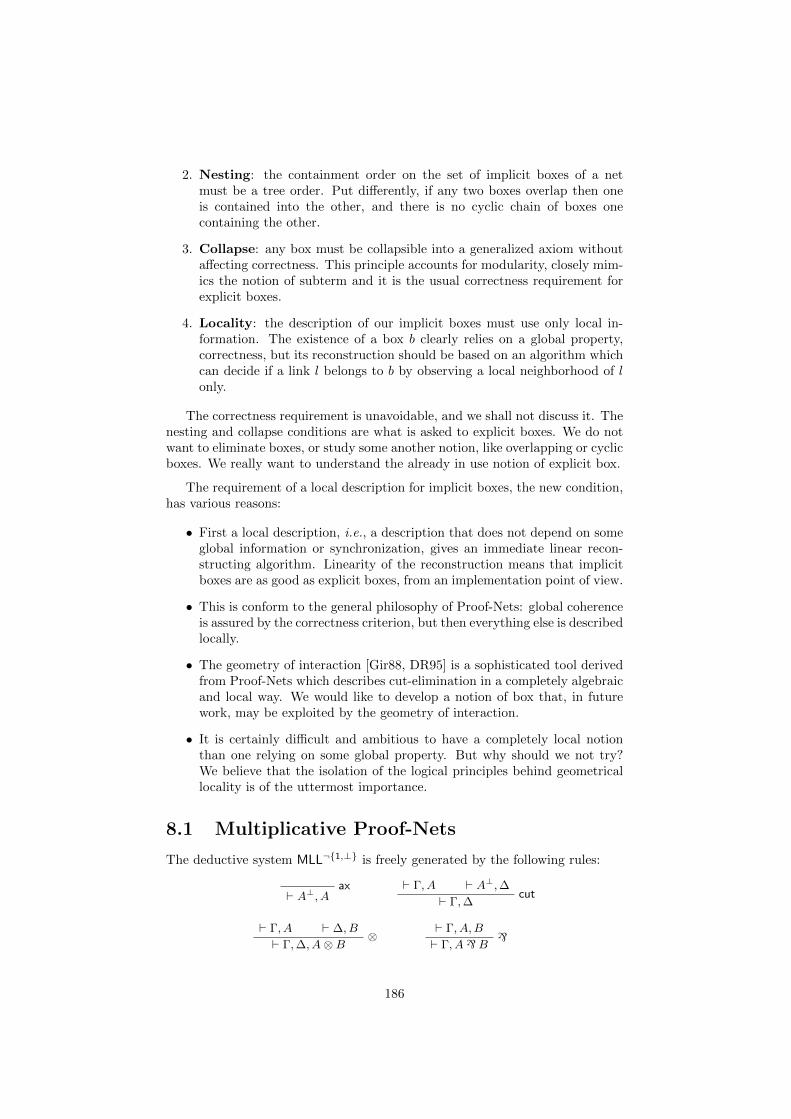
2. Nesting: the containment order on the set of implicit boxes of a netmust be a tree order. Put differently, if any two boxes overlap then oneis contained into the other, and there is no cyclic chain of boxes onecontaining the other.

3. Collapse: any box must be collapsible into a generalized axiom withoutaffecting correctness. This principle accounts for modularity, closely mim-ics the notion of subterm and it is the usual correctness requirement forexplicit boxes.

4. Locality: the description of our implicit boxes must use only local in-formation. The existence of a box b clearly relies on a global property,correctness, but its reconstruction should be based on an algorithm whichcan decide if a link l belongs to b by observing a local neighborhood of lonly.

The correctness requirement is unavoidable, and we shall not discuss it. Thenesting and collapse conditions are what is asked to explicit boxes. We do notwant to eliminate boxes, or study some another notion, like overlapping or cyclicboxes. We really want to understand the already in use notion of explicit box.

The requirement of a local description for implicit boxes, the new condition,has various reasons:

• First a local description, i.e., a description that does not depend on someglobal information or synchronization, gives an immediate linear recon-structing algorithm. Linearity of the reconstruction means that implicitboxes are as good as explicit boxes, from an implementation point of view.

• This is conform to the general philosophy of Proof-Nets: global coherenceis assured by the correctness criterion, but then everything else is describedlocally.

• The geometry of interaction [Gir88, DR95] is a sophisticated tool derivedfrom Proof-Nets which describes cut-elimination in a completely algebraicand local way. We would like to develop a notion of box that, in futurework, may be exploited by the geometry of interaction.

• It is certainly difficult and ambitious to have a completely local notionthan one relying on some global property. But why should we not try?We believe that the isolation of the logical principles behind geometricallocality is of the uttermost importance.

8.1 Multiplicative Proof-Nets

The deductive system MLL¬1,⊥ is freely generated by the following rules:

ax` A⊥, A

` Γ, A ` A⊥,∆cut` Γ,∆

` Γ, A ` ∆, B⊗

` Γ,∆, A⊗B` Γ, A,B

`` Γ, A`B

186

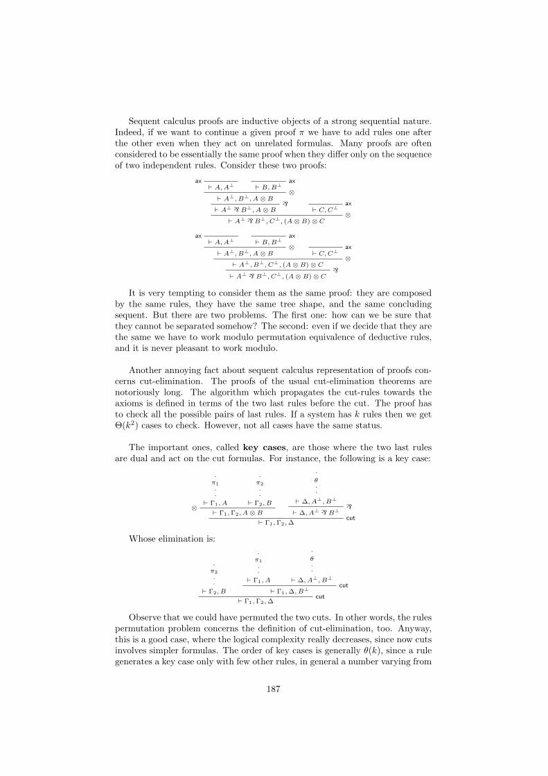
Sequent calculus proofs are inductive objects of a strong sequential nature.Indeed, if we want to continue a given proof π we have to add rules one afterthe other even when they act on unrelated formulas. Many proofs are oftenconsidered to be essentially the same proof when they differ only on the sequenceof two independent rules. Consider these two proofs:

ax` A,A⊥

ax` B,B⊥

⊗` A⊥, B⊥, A⊗ B

`` A⊥ ` B⊥, A⊗ B

ax` C,C⊥

⊗` A⊥ ` B⊥, C⊥, (A⊗ B)⊗ C

ax` A,A⊥

ax` B,B⊥

⊗` A⊥, B⊥, A⊗ B

ax` C,C⊥

⊗` A⊥, B⊥, C⊥, (A⊗ B)⊗ C

`` A⊥ ` B⊥, C⊥, (A⊗ B)⊗ C

It is very tempting to consider them as the same proof: they are composedby the same rules, they have the same tree shape, and the same concludingsequent. But there are two problems. The first one: how can we be sure thatthey cannot be separated somehow? The second: even if we decide that they arethe same we have to work modulo permutation equivalence of deductive rules,and it is never pleasant to work modulo.

Another annoying fact about sequent calculus representation of proofs con-cerns cut-elimination. The proofs of the usual cut-elimination theorems arenotoriously long. The algorithm which propagates the cut-rules towards theaxioms is defined in terms of the two last rules before the cut. The proof hasto check all the possible pairs of last rules. If a system has k rules then we getΘ(k2) cases to check. However, not all cases have the same status.

The important ones, called key cases, are those where the two last rulesare dual and act on the cut formulas. For instance, the following is a key case:

.π1..

` Γ1, A

.π2..

` Γ2, B⊗` Γ1,Γ2, A⊗ B

.

θ..

` ∆, A⊥, B⊥

`` ∆, A⊥ ` B⊥

cut` Γ1,Γ2,∆

Whose elimination is:

.π2..

` Γ2, B

.π1..

` Γ1, A

.

θ..

` ∆, A⊥, B⊥cut

` Γ1,∆, B⊥

cut` Γ1,Γ2,∆

Observe that we could have permuted the two cuts. In other words, the rulespermutation problem concerns the definition of cut-elimination, too. Anyway,this is a good case, where the logical complexity really decreases, since now cutsinvolves simpler formulas. The order of key cases is generally θ(k), since a rulegenerates a key case only with few other rules, in general a number varying from

187

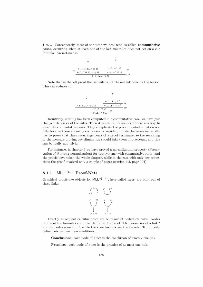
1 to 3. Consequently, most of the time we deal with so-called commutativecases, occurring when at least one of the last two rules does not act on a cutformula. An instance is:

.π..

` Γ, C,D,A⊗ B` ` Γ, C `D,A⊗ B

.

θ..

` ∆, A⊥, B⊥

`` ∆, A⊥ ` B⊥

cut` Γ,∆, C `D

Note that in the left proof the last rule is not the one introducing the tensor.This cut reduces to:

.π..

` Γ, C,D,A⊗ B

.

θ..

` ∆, A⊥, B⊥

`` ∆, A⊥ ` B⊥

cut` Γ,∆, C,D

`` Γ,∆, C `D

Intuitively, nothing has been computed in a commutative case, we have justchanged the order of the rules. Then it is natural to wonder if there is a way toavoid the commutative cases. They complicate the proof of cut-elimination notonly because there are many such cases to consider, but also because one usuallyhas to prove that these re-arrangements of a proof terminate, so the reasoningor the measure proving cut-elimination should take them into account, and thiscan be really non-trivial.

For instance, in chapter 6 we have proved a normalization property (Preser-vation of β-strong normalization) for two systems with commutative rules, andthe proofs have taken the whole chapter, while in the case with only key reduc-tions the proof involved only a couple of pages (section 4.3, page 104).

8.1.1 MLL¬1,⊥ Proof-Nets

Graphical proofs-like objects for MLL¬1,⊥, here called nets, are built out ofthese links:

P⊥ P

axP P⊥

cut

P ⊗ Q

P Q

⊗

N `M

N M

`

Exactly as sequent calculus proof are built out of deduction rules. Nodesrepresent the formulas and links the rules of a proof. The premises of a link lare the nodes source of l, while the conclusions are the targets. To properlydefine nets we need two conditions:

Conclusions: each node of a net is the conclusion of exactly one link.

Premises: each node of a net is the premise of at most one link.

188

'

&

$

%

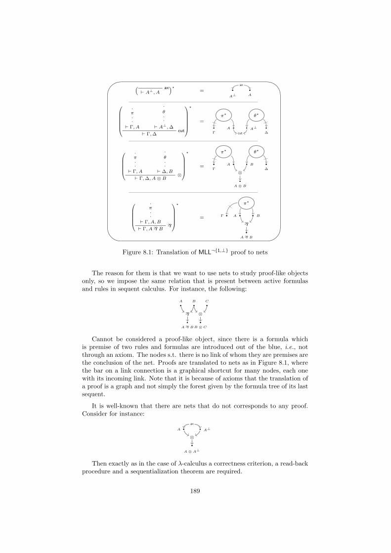
( ax` A⊥, A

)?=

A⊥ A

ax

.π..

` Γ, A

.

θ..

` A⊥,∆cut

` Γ,∆

?

=π?

Γ

A

θ?

∆A⊥

cut

.π..

` Γ, A

.

θ..

` ∆, B⊗

` Γ,∆, A⊗ B

?

=

π?

Γ

A

θ?

∆

B

A ⊗ B

⊗

.π..

` Γ, A,B`` Γ, A` B

?

=

π?

BA

A ` B

`

Γ

Figure 8.1: Translation of MLL¬1,⊥ proof to nets

The reason for them is that we want to use nets to study proof-like objectsonly, so we impose the same relation that is present between active formulasand rules in sequent calculus. For instance, the following:

A B

A ` B

C

B ⊗ C

` ⊗

Cannot be considered a proof-like object, since there is a formula whichis premise of two rules and formulas are introduced out of the blue, i.e., notthrough an axiom. The nodes s.t. there is no link of whom they are premises arethe conclusion of the net. Proofs are translated to nets as in Figure 8.1, wherethe bar on a link connection is a graphical shortcut for many nodes, each onewith its incoming link. Note that it is because of axioms that the translation ofa proof is a graph and not simply the forest given by the formula tree of its lastsequent.

It is well-known that there are nets that do not corresponds to any proof.Consider for instance:

A A⊥

A ⊗ A⊥

ax

⊗

Then exactly as in the case of λ-calculus a correctness criterion, a read-backprocedure and a sequentialization theorem are required.

189

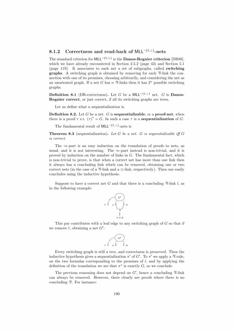
8.1.2 Correctness and read-back of MLL¬1,⊥-nets

The standard criterion for MLL¬1,⊥ is the Danos-Regnier criterion [DR89],which we have already encountered in Section 2.5.2 (page 43) and Section 5.1(page 119). It associates to each net a set of subgraphs, called switchinggraphs. A switching graph is obtained by removing for each `-link the con-nection with one of its premises, choosing arbitrarily, and considering the net asan unoriented graph. If a net G has n `-links then it has 2n possible switchinggraphs.

Definition 8.1 (DR-correctness). Let G be a MLL¬1,⊥ net. G is Danos-Regnier correct, or just correct, if all its switching graphs are trees.

Let us define what a sequentialization is.

Definition 8.2. Let G be a net. G is sequentializable, or a proof-net, whenthere is a proof τ s.t. (τ)

?= G. In such a case τ is a sequentialization of G.

The fundamental result of MLL¬1,⊥-nets is

Theorem 8.3 (sequentialization). Let G be a net. G is sequentializable iff Gis correct.

The ⇒-part is an easy induction on the translation of proofs to nets, asusual, and it is not interesting. The ⇐-part instead is non-trivial, and it isproved by induction on the number of links in G. The fundamental fact, whichis non-trivial to prove, is that when a correct net has more than one link thenit always has a concluding link which can be removed, obtaining one or twocorrect nets (in the case of a `-link and a ⊗-link, respectively). Then one easilyconcludes using the inductive hypothesis.

Suppose to have a correct net G and that there is a concluding `-link l, asin the following example:

G′

BA

A ` B

`

Γ

This par contributes with a leaf edge to any switching graph of G so that ifwe remove l, obtaining a net G′:

G′

BAΓ

Every switching graph is still a tree, and correctness is preserved. Then theinductive hypothesis gives a sequentialization π′ of G′. To π′ we apply a `-rule,on the two formulas corresponding to the premises of l, and by applying thedefinition of the translation we see that π? is exactly G, so we conclude.

The previous reasoning does not depend on G′, hence a concluding `-linkcan always be removed. However, there clearly are proofs where there is noconcluding `. For instance:

190

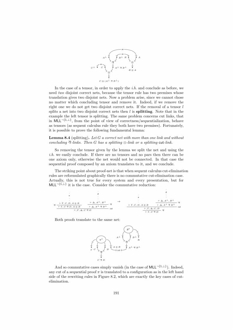
B⊥A⊥

A⊥ ` B⊥

`

B A

B ⊗ A

⊗

ax

ax

CC⊥

C ⊗ (A⊥ ` B⊥)

⊗

ax

In the case of a tensor, in order to apply the i.h. and conclude as before, weneed two disjoint correct nets, because the tensor rule has two premises whosetranslation gives two disjoint nets. Now a problem arise, since we cannot choseno matter which concluding tensor and remove it. Indeed, if we remove theright one we do not get two disjoint correct nets. If the removal of a tensor lsplits a net into two disjoint correct nets then l is splitting. Note that in theexample the left tensor is splitting. The same problem concerns cut links, thatin MLL¬1,⊥, from the point of view of correctness/sequentialization, behaveas tensors (as sequent calculus rule they both have two premises). Fortunately,it is possible to prove the following fundamental lemma:

Lemma 8.4 (splitting). Let G a correct net with more than one link and withoutconcluding `-links. Then G has a splitting ⊗-link or a splitting cut-link.

So removing the tensor given by the lemma we split the net and using thei.h. we easily conclude. If there are no tensors and no pars then there can beone axiom only, otherwise the net would not be connected. In that case thesequential proof composed by an axiom translates to it, and we conclude.

The striking point about proof-net is that when sequent calculus cut-eliminationrules are reformulated graphically there is no commutative cut-elimination case.Actually, this is not true for every system and every presentation, but forMLL¬1,⊥ it is the case. Consider the commutative reduction:

.

π..

` Γ, C,D,A ⊗ B`` Γ, C `D,A ⊗ B

.

θ..

` ∆, A⊥, B⊥`

` ∆, A⊥ ` B⊥cut

`,Γ,∆, C `D

→

.

π..

` Γ, C,D,A ⊗ B

.

θ..

` ∆, A⊥, B⊥`

` ∆, A⊥ ` B⊥cut

`,Γ,∆, C,D`

` Γ, C `D

Both proofs translate to the same net:

π?

Γ

A ⊗ BC D

C `D

`

A⊥ ` B⊥

B⊥A⊥

`

θ?

∆

cut

And so commutative cases simply vanish (in the case of MLL¬1,⊥). Indeed,any cut of a sequential proof π is translated to a configuration as in the left handside of the rewriting rules in Figure 8.2, which are exactly the key cases of cut-elimination.

191

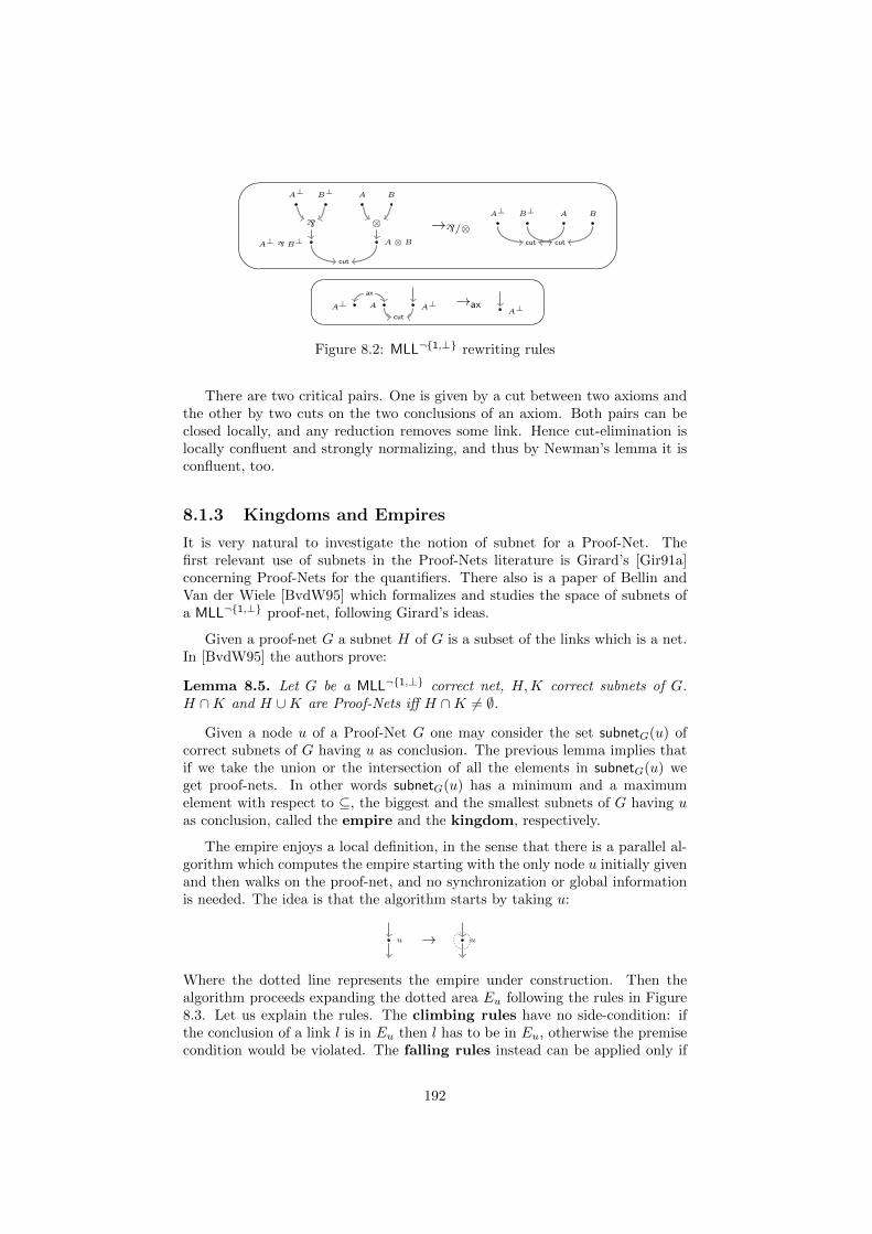
A ⊗ B

A B

⊗

A⊥ ` B⊥

A⊥ B⊥

`

cut

→`/⊗A BB⊥A⊥

cut cut

A⊥AA⊥

ax

cut

→axA⊥

Figure 8.2: MLL¬1,⊥ rewriting rules

There are two critical pairs. One is given by a cut between two axioms andthe other by two cuts on the two conclusions of an axiom. Both pairs can beclosed locally, and any reduction removes some link. Hence cut-elimination islocally confluent and strongly normalizing, and thus by Newman’s lemma it isconfluent, too.

8.1.3 Kingdoms and Empires

It is very natural to investigate the notion of subnet for a Proof-Net. Thefirst relevant use of subnets in the Proof-Nets literature is Girard’s [Gir91a]concerning Proof-Nets for the quantifiers. There also is a paper of Bellin andVan der Wiele [BvdW95] which formalizes and studies the space of subnets ofa MLL¬1,⊥ proof-net, following Girard’s ideas.

Given a proof-net G a subnet H of G is a subset of the links which is a net.In [BvdW95] the authors prove:

Lemma 8.5. Let G be a MLL¬1,⊥ correct net, H,K correct subnets of G.H ∩K and H ∪K are Proof-Nets iff H ∩K 6= ∅.

Given a node u of a Proof-Net G one may consider the set subnetG(u) ofcorrect subnets of G having u as conclusion. The previous lemma implies thatif we take the union or the intersection of all the elements in subnetG(u) weget proof-nets. In other words subnetG(u) has a minimum and a maximumelement with respect to ⊆, the biggest and the smallest subnets of G having uas conclusion, called the empire and the kingdom, respectively.

The empire enjoys a local definition, in the sense that there is a parallel al-gorithm which computes the empire starting with the only node u initially givenand then walks on the proof-net, and no synchronization or global informationis needed. The idea is that the algorithm starts by taking u:

u → u

Where the dotted line represents the empire under construction. Then thealgorithm proceeds expanding the dotted area Eu following the rules in Figure8.3. Let us explain the rules. The climbing rules have no side-condition: ifthe conclusion of a link l is in Eu then l has to be in Eu, otherwise the premisecondition would be violated. The falling rules instead can be applied only if

192

'

&

$

%

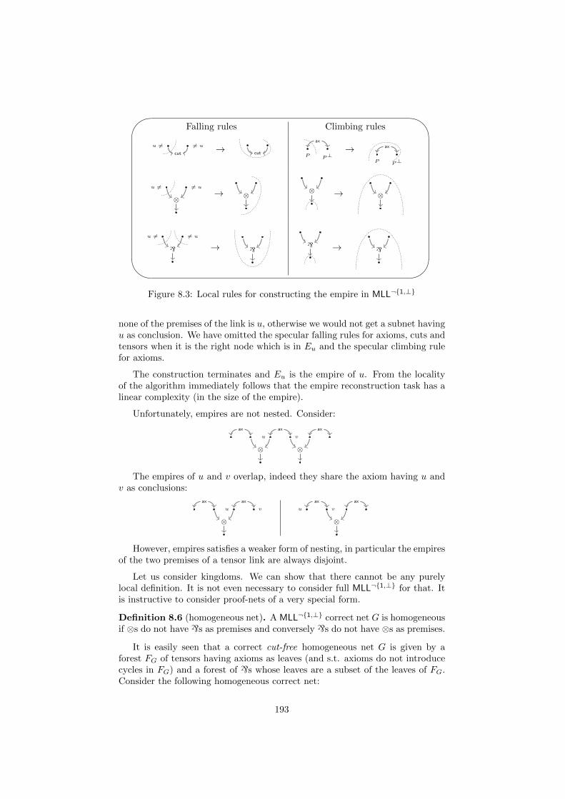
Falling rules Climbing rules

u 6= 6= u

cut→ cut

P P⊥

ax

→P P⊥

ax

u 6= 6= u

⊗→ ⊗

⊗ → ⊗

u 6= 6= u

` → `` → `

Figure 8.3: Local rules for constructing the empire in MLL¬1,⊥

none of the premises of the link is u, otherwise we would not get a subnet havingu as conclusion. We have omitted the specular falling rules for axioms, cuts andtensors when it is the right node which is in Eu and the specular climbing rulefor axioms.

The construction terminates and Eu is the empire of u. From the localityof the algorithm immediately follows that the empire reconstruction task has alinear complexity (in the size of the empire).

Unfortunately, empires are not nested. Consider:

ax

u v

ax ax

⊗ ⊗

The empires of u and v overlap, indeed they share the axiom having u andv as conclusions:

ax

u v

ax

⊗

u v

ax ax

⊗

However, empires satisfies a weaker form of nesting, in particular the empiresof the two premises of a tensor link are always disjoint.

Let us consider kingdoms. We can show that there cannot be any purelylocal definition. It is not even necessary to consider full MLL¬1,⊥ for that. Itis instructive to consider proof-nets of a very special form.

Definition 8.6 (homogeneous net). A MLL¬1,⊥ correct net G is homogeneousif ⊗s do not have `s as premises and conversely `s do not have ⊗s as premises.

It is easily seen that a correct cut-free homogeneous net G is given by aforest FG of tensors having axioms as leaves (and s.t. axioms do not introducecycles in FG) and a forest of `s whose leaves are a subset of the leaves of FG.Consider the following homogeneous correct net:

193

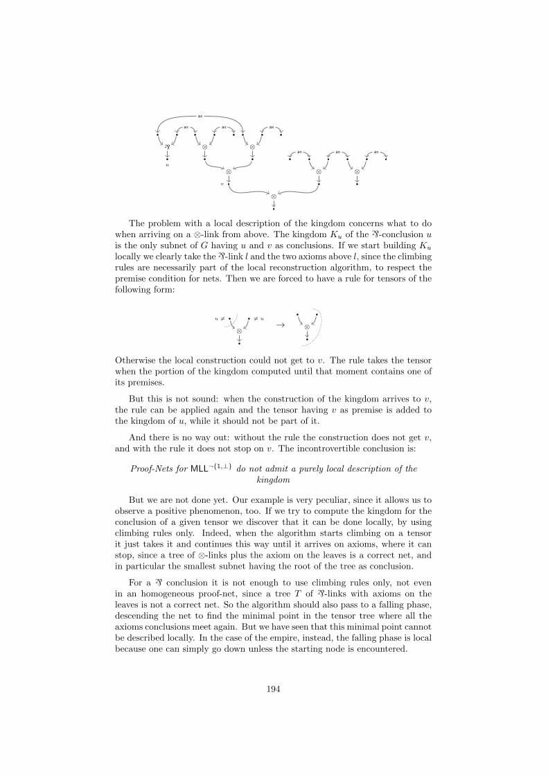
axax

ax

v

⊗ ⊗

⊗⊗

⊗

ax

u

`

⊗

ax

ax

ax

The problem with a local description of the kingdom concerns what to dowhen arriving on a ⊗-link from above. The kingdom Ku of the `-conclusion uis the only subnet of G having u and v as conclusions. If we start building Ku

locally we clearly take the`-link l and the two axioms above l, since the climbingrules are necessarily part of the local reconstruction algorithm, to respect thepremise condition for nets. Then we are forced to have a rule for tensors of thefollowing form:

u 6= 6= u

⊗→ ⊗

Otherwise the local construction could not get to v. The rule takes the tensorwhen the portion of the kingdom computed until that moment contains one ofits premises.

But this is not sound: when the construction of the kingdom arrives to v,the rule can be applied again and the tensor having v as premise is added tothe kingdom of u, while it should not be part of it.

And there is no way out: without the rule the construction does not get v,and with the rule it does not stop on v. The incontrovertible conclusion is:

Proof-Nets for MLL¬1,⊥ do not admit a purely local description of thekingdom

But we are not done yet. Our example is very peculiar, since it allows us toobserve a positive phenomenon, too. If we try to compute the kingdom for theconclusion of a given tensor we discover that it can be done locally, by usingclimbing rules only. Indeed, when the algorithm starts climbing on a tensorit just takes it and continues this way until it arrives on axioms, where it canstop, since a tree of ⊗-links plus the axiom on the leaves is a correct net, andin particular the smallest subnet having the root of the tree as conclusion.

For a ` conclusion it is not enough to use climbing rules only, not evenin an homogeneous proof-net, since a tree T of `-links with axioms on theleaves is not a correct net. So the algorithm should also pass to a falling phase,descending the net to find the minimal point in the tensor tree where all theaxioms conclusions meet again. But we have seen that this minimal point cannotbe described locally. In the case of the empire, instead, the falling phase is localbecause one can simply go down unless the starting node is encountered.

194

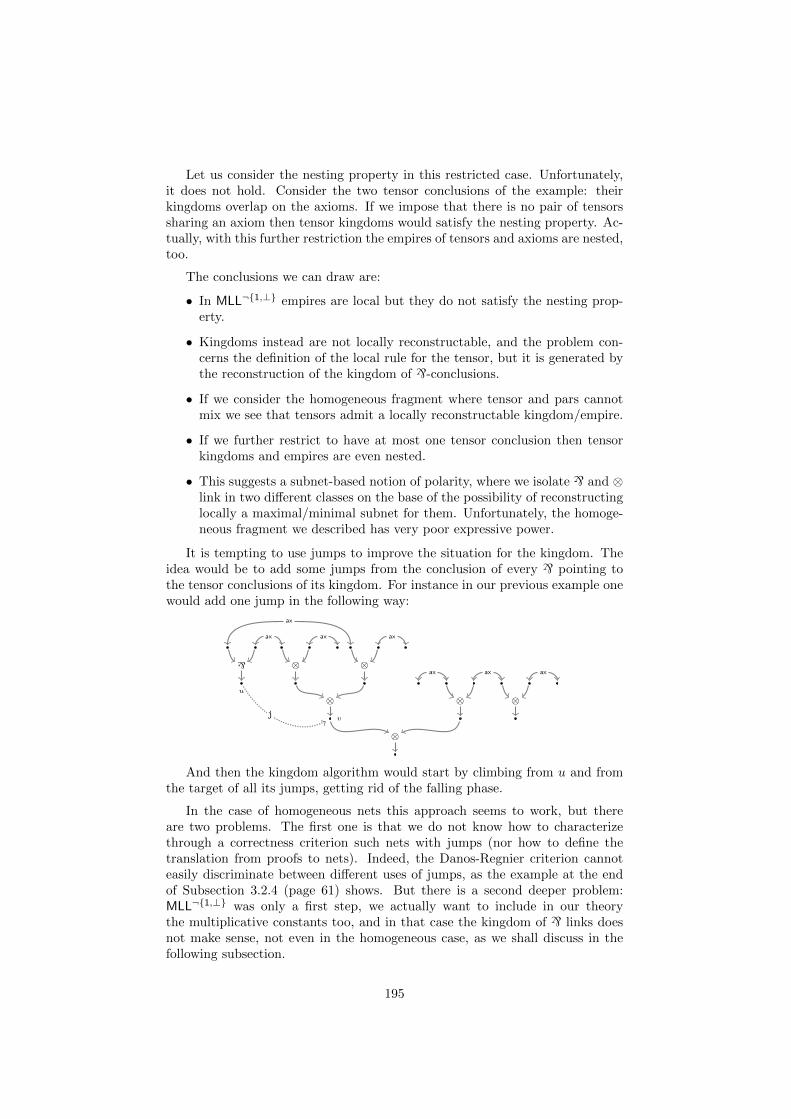
Let us consider the nesting property in this restricted case. Unfortunately,it does not hold. Consider the two tensor conclusions of the example: theirkingdoms overlap on the axioms. If we impose that there is no pair of tensorssharing an axiom then tensor kingdoms would satisfy the nesting property. Ac-tually, with this further restriction the empires of tensors and axioms are nested,too.

The conclusions we can draw are:

• In MLL¬1,⊥ empires are local but they do not satisfy the nesting prop-erty.

• Kingdoms instead are not locally reconstructable, and the problem con-cerns the definition of the local rule for the tensor, but it is generated bythe reconstruction of the kingdom of `-conclusions.

• If we consider the homogeneous fragment where tensor and pars cannotmix we see that tensors admit a locally reconstructable kingdom/empire.

• If we further restrict to have at most one tensor conclusion then tensorkingdoms and empires are even nested.

• This suggests a subnet-based notion of polarity, where we isolate ` and ⊗link in two different classes on the base of the possibility of reconstructinglocally a maximal/minimal subnet for them. Unfortunately, the homoge-neous fragment we described has very poor expressive power.

It is tempting to use jumps to improve the situation for the kingdom. Theidea would be to add some jumps from the conclusion of every ` pointing tothe tensor conclusions of its kingdom. For instance in our previous example onewould add one jump in the following way:

axax

ax

v

⊗ ⊗

⊗⊗

⊗

ax

u

`

⊗

ax

ax

ax

j

And then the kingdom algorithm would start by climbing from u and fromthe target of all its jumps, getting rid of the falling phase.

In the case of homogeneous nets this approach seems to work, but thereare two problems. The first one is that we do not know how to characterizethrough a correctness criterion such nets with jumps (nor how to define thetranslation from proofs to nets). Indeed, the Danos-Regnier criterion cannoteasily discriminate between different uses of jumps, as the example at the endof Subsection 3.2.4 (page 61) shows. But there is a second deeper problem:MLL¬1,⊥ was only a first step, we actually want to include in our theorythe multiplicative constants too, and in that case the kingdom of ` links doesnot make sense, not even in the homogeneous case, as we shall discuss in thefollowing subsection.

195

(

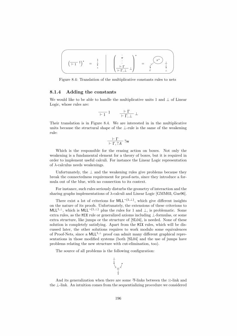
1` 1

)?=

1

1

.π..

` Γ ⊥` Γ,⊥

?

=π?

Γ ⊥

⊥

Figure 8.4: Translation of the multiplicative constants rules to nets

8.1.4 Adding the constants

We would like to be able to handle the multiplicative units 1 and ⊥ of LinearLogic, whose rules are:

1` 1` Γ ⊥` Γ,⊥

Their translation is in Figure 8.4. We are interested in in the multiplicativeunits because the structural shape of the ⊥-rule is the same of the weakeningrule:

` Γ?w` Γ, ?A

Which is the responsible for the erasing action on boxes. Not only theweakening is a fundamental element for a theory of boxes, but it is required inorder to implement useful calculi. For instance the Linear Logic representationof λ-calculus needs weakenings.

Unfortunately, the ⊥ and the weakening rules give problems because theybreak the connectedness requirement for proof-nets, since they introduce a for-mula out of the blue, with no connection to its context.

For instance, such rules seriously disturbs the geometry of interaction and thesharing graphs implementations of λ-calculi and Linear Logic [GMM03, Gue96].

There exist a lot of criterions for MLL¬1,⊥, which give different insightson the nature of its proofs. Unfortunately, the extensions of these criterions toMLL1,⊥, which is MLL¬1,⊥ plus the rules for 1 and ⊥, is problematic. Someextra rules, as the MIX rule or generalized axioms including ⊥-formulas, or someextra structure, like jumps or the structure of [SL04], is needed. None of thesesolution is completely satisfying. Apart from the MIX rules, which will be dis-cussed later, the other solutions requires to work modulo some equivalencesof Proof-Nets, since a MLL1,⊥ proof can admit many different graphical repre-sentations in those modified systems (both [SL04] and the use of jumps haveproblems relating the new structure with cut-elimination, too).

The source of all problems is the following configuration:

⊗

⊥

And its generalization when there are some `-links between the ⊗-link andthe ⊥-link. An intuition comes from the sequentializing procedure we considered

196

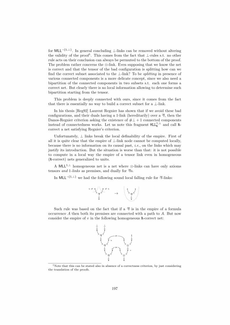
for MLL¬1,⊥. In general concluding ⊥-links can be removed without alteringthe validity of the proof1. This comes from the fact that ⊥-rules s.t. no otherrule acts on their conclusion can always be permuted to the bottom of the proof.The problem rather concerns the ⊗-link. Even supposing that we know the netis correct and that the tensor of the bad configuration is splitting how can wefind the correct subnet associated to the ⊥-link? To be splitting in presence ofvarious connected components is a more delicate concept, since we also need abipartition of the connected components in two subsets s.t. each one forms acorrect net. But clearly there is no local information allowing to determine suchbipartition starting from the tensor.

This problem is deeply connected with ours, since it comes from the factthat there is essentially no way to build a correct subnet for a ⊥-link.

In his thesis [Reg92] Laurent Regnier has shown that if we avoid these badconfigurations, and their duals having a 1-link (hereditarily) over a `, then theDanos-Regnier criterion asking the existence of #⊥+ 1 connected componentsinstead of connectedness works. Let us note this fragment MLL

1,⊥R and call R-

correct a net satisfying Regnier’s criterion.

Unfortunately, ⊥ links break the local definability of the empire. First ofall it is quite clear that the empire of ⊥-link node cannot be computed locally,because there is no information on its causal past, i.e., on the links which mayjustify its introduction. But the situation is worse than that: it is not possibleto compute in a local way the empire of a tensor link even in homogeneous(R-correct) nets generalized to units.

A MLL1,⊥ homogeneous net is a net where ⊗-links can have only axiomstensors and 1-links as premises, and dually for `s.

In MLL¬1,⊥ we had the following sound local falling rule for `-links:

u 6= 6= u

` → `

Such rule was based on the fact that if a ` is in the empire of a formulaoccurrence A then both its premises are connected with a path to A. But nowconsider the empire of v in the following homogeneous R-correct net:

`

⊥ ⊥

u

`

`

ax

v

⊗

⊗

1ax

1Note that this can be stated also in absence of a correctness criterion, by just consideringthe translation of the proofs.

197

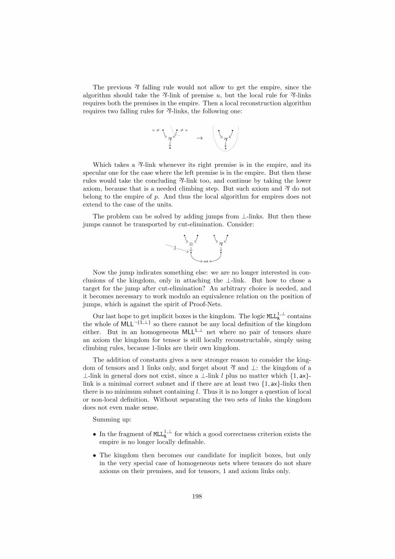
The previous ` falling rule would not allow to get the empire, since thealgorithm should take the `-link of premise u, but the local rule for `-linksrequires both the premises in the empire. Then a local reconstruction algorithmrequires two falling rules for `-links, the following one:

u 6= 6= u

` → `

Which takes a `-link whenever its right premise is in the empire, and itsspecular one for the case where the left premise is in the empire. But then theserules would take the concluding `-link too, and continue by taking the loweraxiom, because that is a needed climbing step. But such axiom and ` do notbelong to the empire of p. And thus the local algorithm for empires does notextend to the case of the units.

The problem can be solved by adding jumps from ⊥-links. But then thesejumps cannot be transported by cut-elimination. Consider:

`⊗

cut

j

Now the jump indicates something else: we are no longer interested in con-clusions of the kingdom, only in attaching the ⊥-link. But how to chose atarget for the jump after cut-elimination? An arbitrary choice is needed, andit becomes necessary to work modulo an equivalence relation on the position ofjumps, which is against the spirit of Proof-Nets.

Our last hope to get implicit boxes is the kingdom. The logic MLL1,⊥R contains

the whole of MLL¬1,⊥ so there cannot be any local definition of the kingdomeither. But in an homogeneous MLL1,⊥ net where no pair of tensors sharean axiom the kingdom for tensor is still locally reconstructable, simply usingclimbing rules, because 1-links are their own kingdom.

The addition of constants gives a new stronger reason to consider the king-dom of tensors and 1 links only, and forget about ` and ⊥: the kingdom of a⊥-link in general does not exist, since a ⊥-link l plus no matter which 1, ax-link is a minimal correct subnet and if there are at least two 1, ax-links thenthere is no minimum subnet containing l. Thus it is no longer a question of localor non-local definition. Without separating the two sets of links the kingdomdoes not even make sense.

Summing up:

• In the fragment of MLL1,⊥R for which a good correctness criterion exists the

empire is no longer locally definable.

• The kingdom then becomes our candidate for implicit boxes, but onlyin the very special case of homogeneous nets where tensors do not shareaxioms on their premises, and for tensors, 1 and axiom links only.

198

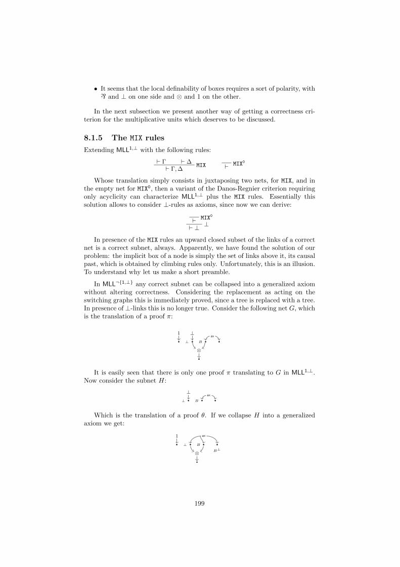
• It seems that the local definability of boxes requires a sort of polarity, with` and ⊥ on one side and ⊗ and 1 on the other.

In the next subsection we present another way of getting a correctness cri-terion for the multiplicative units which deserves to be discussed.

8.1.5 The MIX rules

Extending MLL1,⊥ with the following rules:

` Γ ` ∆MIX` Γ,∆

MIX0`

Whose translation simply consists in juxtaposing two nets, for MIX, and inthe empty net for MIX0, then a variant of the Danos-Regnier criterion requiringonly acyclicity can characterize MLL1,⊥ plus the MIX rules. Essentially thissolution allows to consider ⊥-rules as axioms, since now we can derive:

MIX0` ⊥` ⊥

In presence of the MIX rules an upward closed subset of the links of a correctnet is a correct subnet, always. Apparently, we have found the solution of ourproblem: the implicit box of a node is simply the set of links above it, its causalpast, which is obtained by climbing rules only. Unfortunately, this is an illusion.To understand why let us make a short preamble.

In MLL¬1,⊥ any correct subnet can be collapsed into a generalized axiomwithout altering correctness. Considering the replacement as acting on theswitching graphs this is immediately proved, since a tree is replaced with a tree.In presence of ⊥-links this is no longer true. Consider the following net G, whichis the translation of a proof π:

B

ax

⊥

⊥1

⊗

It is easily seen that there is only one proof π translating to G in MLL1,⊥.Now consider the subnet H:

B

ax

⊥

⊥

Which is the translation of a proof θ. If we collapse H into a generalizedaxiom we get:

B

B⊥⊥

1 ax

⊗

199

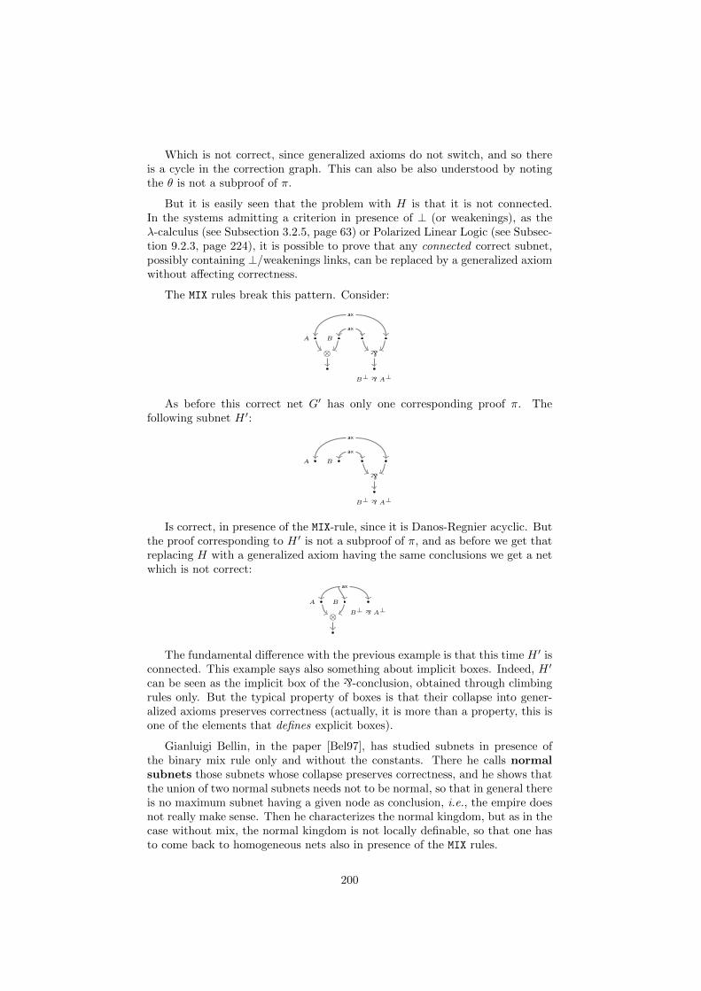
Which is not correct, since generalized axioms do not switch, and so thereis a cycle in the correction graph. This can also be also understood by notingthe θ is not a subproof of π.

But it is easily seen that the problem with H is that it is not connected.In the systems admitting a criterion in presence of ⊥ (or weakenings), as theλ-calculus (see Subsection 3.2.5, page 63) or Polarized Linear Logic (see Subsec-tion 9.2.3, page 224), it is possible to prove that any connected correct subnet,possibly containing ⊥/weakenings links, can be replaced by a generalized axiomwithout affecting correctness.

The MIX rules break this pattern. Consider:

B

ax

A

ax

B⊥ ` A⊥

`⊗

As before this correct net G′ has only one corresponding proof π. Thefollowing subnet H ′:

B

ax

A

ax

B⊥ ` A⊥

`

Is correct, in presence of the MIX-rule, since it is Danos-Regnier acyclic. Butthe proof corresponding to H ′ is not a subproof of π, and as before we get thatreplacing H with a generalized axiom having the same conclusions we get a netwhich is not correct:

B

B⊥ ` A⊥A

ax

⊗

The fundamental difference with the previous example is that this time H ′ isconnected. This example says also something about implicit boxes. Indeed, H ′

can be seen as the implicit box of the `-conclusion, obtained through climbingrules only. But the typical property of boxes is that their collapse into gener-alized axioms preserves correctness (actually, it is more than a property, this isone of the elements that defines explicit boxes).

Gianluigi Bellin, in the paper [Bel97], has studied subnets in presence ofthe binary mix rule only and without the constants. There he calls normalsubnets those subnets whose collapse preserves correctness, and he shows thatthe union of two normal subnets needs not to be normal, so that in general thereis no maximum subnet having a given node as conclusion, i.e., the empire doesnot really make sense. Then he characterizes the normal kingdom, but as in thecase without mix, the normal kingdom is not locally definable, so that one hasto come back to homogeneous nets also in presence of the MIX rules.

200

To sum up the MIX-rules give a correctness criterion but they do not changethe fact that to have an implicit and local notion of box we need to considerconstrained homogeneous nets. But as far as homogeneous nets are consideredit is possible to use Regnier’s criterion, and there is no need of the MIX-rules.

This property of being collapsible preserving correctness is a further impor-tant requirement for implicit boxes. It is a topological property which accountsfor modularity.

To conclude, it seems that in presence of the units there is no possibletheory of local implicit boxes unless one reduces to consider the separation ofconnectives at work in the homogeneous fragment.

This fragment is very weak, since there is no way of mixing ⊥,`-linkswith 1,⊗-links except than through cuts. But fortunately it is contained in alogic with exponentials, Multiplicative and Exponential Polarized Linear Logic(MELLP), where expressivity is recovered by introducing both the exponentialconnectives and a rigid way of mixing the two set of connectives.

8.2 MELLP

Multiplicative and Exponential Polarized Linear Logic (MELLP) has been intro-duced and studied in depth by Olivier Laurent [Lau02]. The original motivationbehind this system have nothing to do with the reconstruction of boxes. Indeed,it rather came out as a proof theoretical by-product of Jean-Yves Girard’s in-vestigation of Classical Logic through Linear Logic [Gir91b]. The main resultof this second part of the thesis is that MELLP Proof-Nets can be reformulatedso that positive formula nodes enjoy implicit boxes.

We shall proceed gradually. In this section we introduce the Laurent’s pre-sentation of MELLP and the corresponding Proof-Nets, which use explicit boxes.In the next two chapters we shall revisit MELLP proof nets in order to get im-plicit boxes.

For a more comprehensive presentation and study of MELLP we refer thereader to Laurent’s PhD thesis [Lau02].

8.2.1 The system

In MELLP the restrictions separating tensors and 1s with respect to `s and ⊥s,and the fact that tensors do not share the eventual axioms on their premiseare hardcoded into the proof system through a notion of polarity. The systemincludes the exponentials so it is much more expressive of what we have consid-ered so far, indeed there are translation of the λ-calculus and of the λµ-calculusin MELLP [Lau02].

The formulas of MELLP are given by two mutually defined sets, positiveand negative formulas, denoted respectively with P,Q and N,M :

P,Q ::= X | 1 | P ⊗Q | !NN,M ::= X⊥ | ⊥ | N `M | ?P

The positive formulas contain those for which we have a notion of implicitbox, while the negative ones contain the dual formulas. But there also is a

201

'

&

$

%

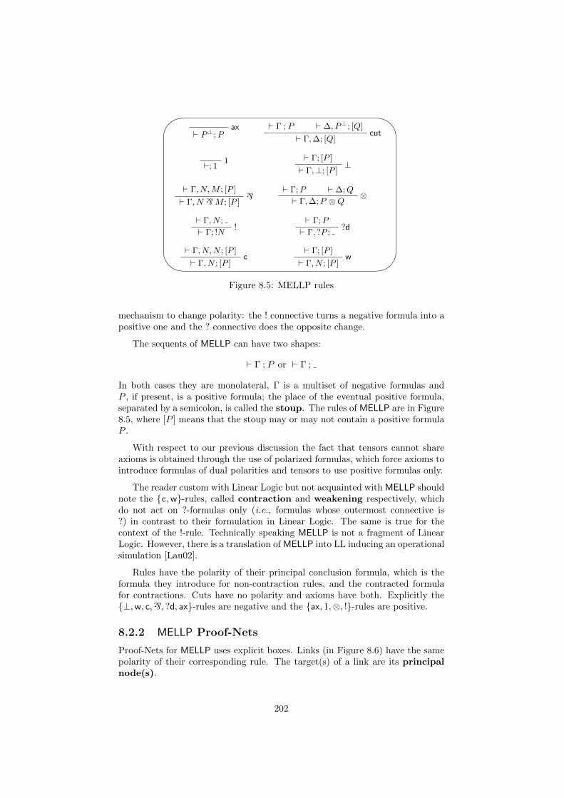
ax` P⊥;P

` Γ ; P ` ∆, P⊥; [Q]cut

` Γ,∆; [Q]

1`; 1` Γ; [P ]

⊥` Γ,⊥; [P ]

` Γ, N,M ; [P ]`` Γ, N `M ; [P ]

` Γ;P ` ∆;Q⊗

` Γ,∆;P ⊗Q

` Γ, N ;!` Γ; !N

` Γ;P?d` Γ, ?P ;

` Γ, N,N ; [P ]c

` Γ, N ; [P ]

` Γ; [P ]w

` Γ, N ; [P ]

Figure 8.5: MELLP rules

mechanism to change polarity: the ! connective turns a negative formula into apositive one and the ? connective does the opposite change.

The sequents of MELLP can have two shapes:

` Γ ; P or ` Γ ;

In both cases they are monolateral, Γ is a multiset of negative formulas andP , if present, is a positive formula; the place of the eventual positive formula,separated by a semicolon, is called the stoup. The rules of MELLP are in Figure8.5, where [P ] means that the stoup may or may not contain a positive formulaP .

With respect to our previous discussion the fact that tensors cannot shareaxioms is obtained through the use of polarized formulas, which force axioms tointroduce formulas of dual polarities and tensors to use positive formulas only.

The reader custom with Linear Logic but not acquainted with MELLP shouldnote the c,w-rules, called contraction and weakening respectively, whichdo not act on ?-formulas only (i.e., formulas whose outermost connective is?) in contrast to their formulation in Linear Logic. The same is true for thecontext of the !-rule. Technically speaking MELLP is not a fragment of LinearLogic. However, there is a translation of MELLP into LL inducing an operationalsimulation [Lau02].

Rules have the polarity of their principal conclusion formula, which is theformula they introduce for non-contraction rules, and the contracted formulafor contractions. Cuts have no polarity and axioms have both. Explicitly the⊥,w, c,`, ?d, ax-rules are negative and the ax, 1,⊗, !-rules are positive.

8.2.2 MELLP Proof-Nets

Proof-Nets for MELLP uses explicit boxes. Links (in Figure 8.6) have the samepolarity of their corresponding rule. The target(s) of a link are its principalnode(s).

202

'

&

$

%

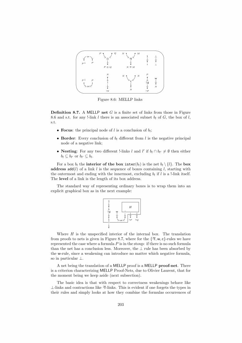
P⊥ P

ax

P ⊗ Q

P Q

⊗

N `M

N M

`1

1

⊥

⊥

P⊥ P

cut

!N

N

!

N

N N

c

?P

P

?d

N

w

Figure 8.6: MELLP links

Definition 8.7. A MELLP net G is a finite set of links from those in Figure8.6 and s.t. for any !-link l there is an associated subnet bl of G, the box of l,s.t.

• Focus: the principal node of l is a conclusion of bl;

• Border: Every conclusion of bl different from l is the negative principalnode of a negative link;

• Nesting: For any two different !-links l and l′ if bl ∩ bl′ 6= ∅ then eitherbl ⊆ bl′ or bl′ ⊆ bl.

For a box bl the interior of the box inter(bl) is the net bl \ l. The boxaddress add(l) of a link l is the sequence of boxes containing l, starting withthe outermost and ending with the innermost, excluding bl if l is a !-link itself.The level of a link is the length of its box address.

The standard way of representing ordinary boxes is to wrap them into anexplicit graphical box as in the next example:

w

1

?d !

?Q?P

H

!cut

Where H is the unspecified interior of the internal box. The translationfrom proofs to nets is given in Figure 8.7, where for the `,w, c-rules we haverepresented the case where a formula P is in the stoup: if there is no such formulathan the net has a conclusion less. Moreover, the ⊥ rule has been absorbed bythe w-rule, since a weakening can introduce no matter which negative formula,so in particular ⊥.

A net being the translation of a MELLP proof is a MELLP proof-net. Thereis a criterion characterizing MELLP Proof-Nets, due to Olivier Laurent, that forthe moment being we keep aside (next subsection).

The basic idea is that with respect to correctness weakenings behave like⊥-links and contractions like `-links. This is evident if one forgets the types intheir rules and simply looks at how they combine the formulas occurrences of

203

'

&

$

%

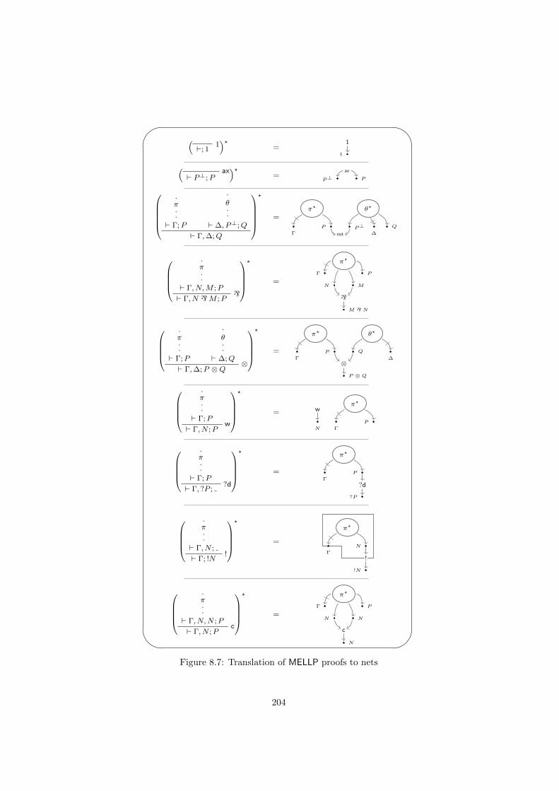
(1`; 1

)?=

1

1

(ax

` P⊥;P

)?=

P⊥ P

ax

.π..

` Γ;P

.

θ..

` ∆, P⊥;Q

` Γ,∆;Q

?

=π?

Γ

P

θ?

P⊥∆

Q

cut

.π..

` Γ, N,M ;P`` Γ, N `M ;P

?

=

π?

MN

Γ P

M ` N

`

.π..

` Γ;P

.

θ..

` ∆;Q⊗

` Γ,∆;P ⊗Q

?

=

π?

Γ

P

θ?

∆

Q

P ⊗ Q

⊗

.π..

` Γ;Pw

` Γ, N ;P

?

=π?

Γ

P

N

w

.π..

` Γ;P?d` Γ, ?P ;

?

=

π?

Γ

P

?P

?d

.π..

` Γ, N ;!` Γ; !N

?

=

π?

Γ

N

!N

!

.π..

` Γ, N,N ;Pc

` Γ, N ;P

?

=

π?

NN

Γ P

N

c

Figure 8.7: Translation of MELLP proofs to nets

204

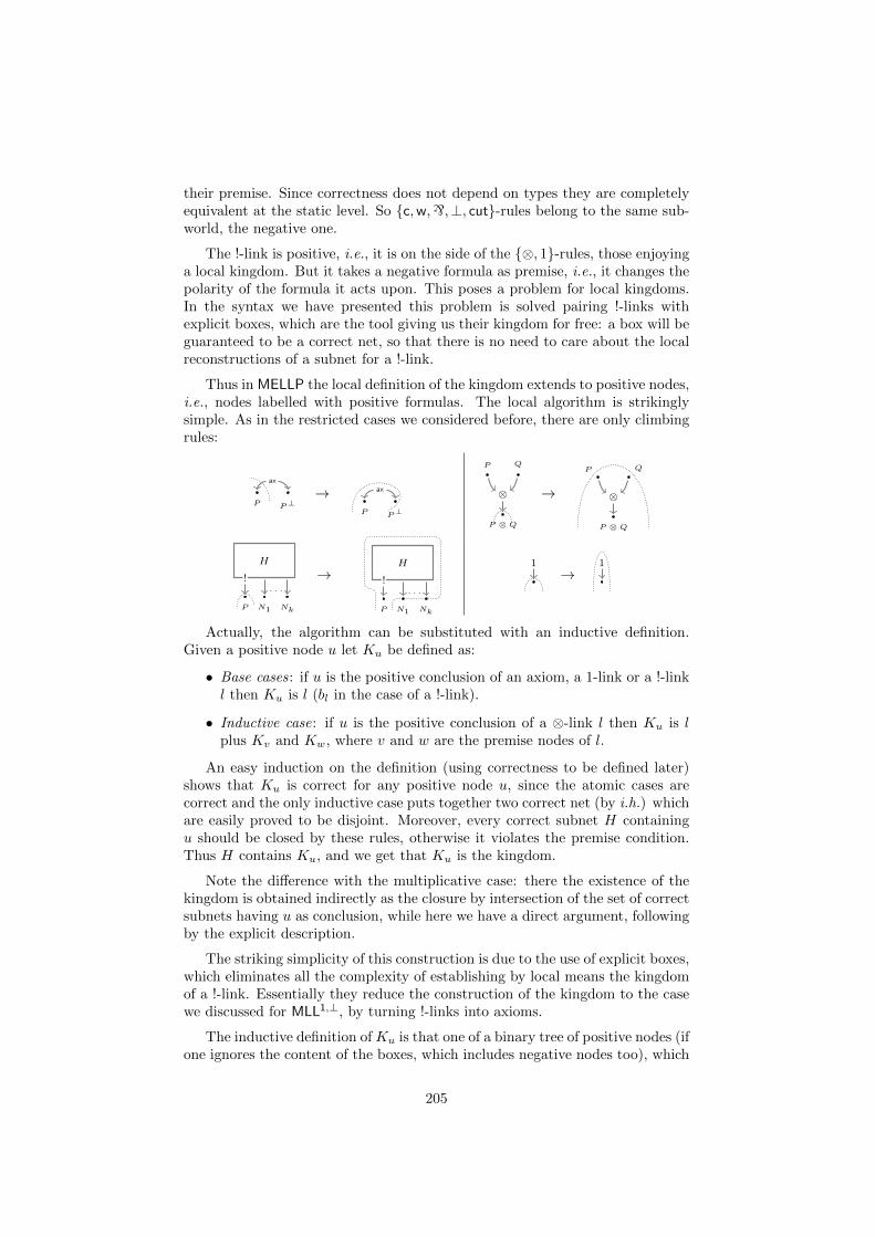
their premise. Since correctness does not depend on types they are completelyequivalent at the static level. So c,w,`,⊥, cut-rules belong to the same sub-world, the negative one.

The !-link is positive, i.e., it is on the side of the ⊗, 1-rules, those enjoyinga local kingdom. But it takes a negative formula as premise, i.e., it changes thepolarity of the formula it acts upon. This poses a problem for local kingdoms.In the syntax we have presented this problem is solved pairing !-links withexplicit boxes, which are the tool giving us their kingdom for free: a box will beguaranteed to be a correct net, so that there is no need to care about the localreconstructions of a subnet for a !-link.

Thus in MELLP the local definition of the kingdom extends to positive nodes,i.e., nodes labelled with positive formulas. The local algorithm is strikinglysimple. As in the restricted cases we considered before, there are only climbingrules:

P P⊥

ax

→P P⊥

ax

P Q

P ⊗ Q

⊗ →

P Q

P ⊗ Q

⊗

P

!

NkN1

H

. . .

→

P

!

NkN1

H

. . .

1

→1

Actually, the algorithm can be substituted with an inductive definition.Given a positive node u let Ku be defined as:

• Base cases: if u is the positive conclusion of an axiom, a 1-link or a !-linkl then Ku is l (bl in the case of a !-link).

• Inductive case: if u is the positive conclusion of a ⊗-link l then Ku is lplus Kv and Kw, where v and w are the premise nodes of l.

An easy induction on the definition (using correctness to be defined later)shows that Ku is correct for any positive node u, since the atomic cases arecorrect and the only inductive case puts together two correct net (by i.h.) whichare easily proved to be disjoint. Moreover, every correct subnet H containingu should be closed by these rules, otherwise it violates the premise condition.Thus H contains Ku, and we get that Ku is the kingdom.

Note the difference with the multiplicative case: there the existence of thekingdom is obtained indirectly as the closure by intersection of the set of correctsubnets having u as conclusion, while here we have a direct argument, followingby the explicit description.

The striking simplicity of this construction is due to the use of explicit boxes,which eliminates all the complexity of establishing by local means the kingdomof a !-link. Essentially they reduce the construction of the kingdom to the casewe discussed for MLL1,⊥, by turning !-links into axioms.

The inductive definition of Ku is that one of a binary tree of positive nodes (ifone ignores the content of the boxes, which includes negative nodes too), which

205

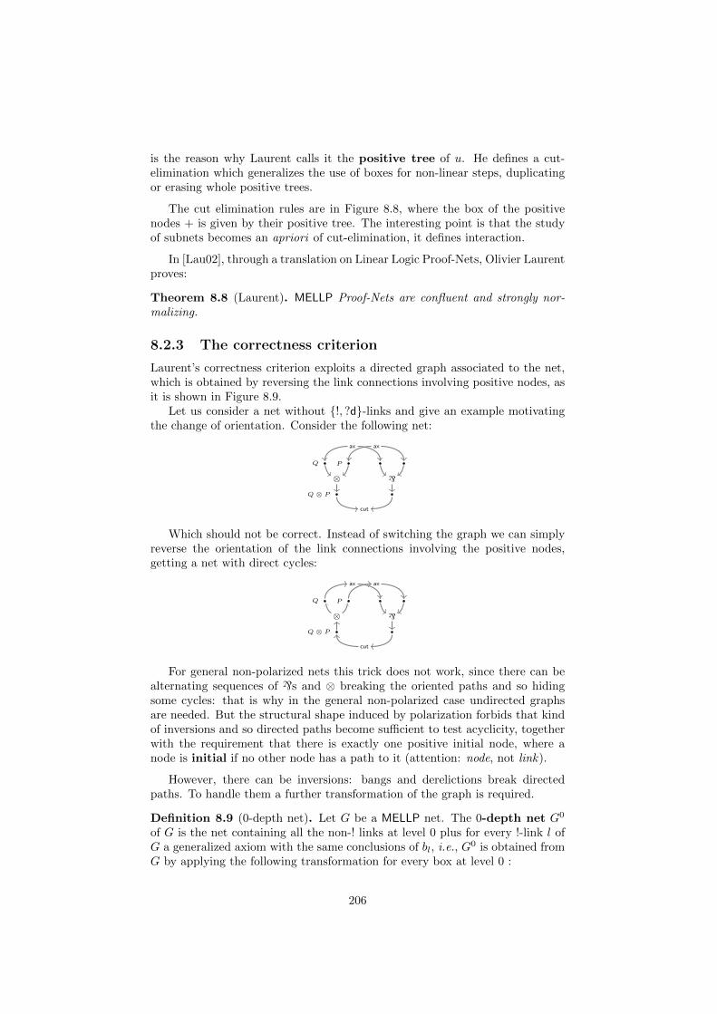
is the reason why Laurent calls it the positive tree of u. He defines a cut-elimination which generalizes the use of boxes for non-linear steps, duplicatingor erasing whole positive trees.

The cut elimination rules are in Figure 8.8, where the box of the positivenodes + is given by their positive tree. The interesting point is that the studyof subnets becomes an apriori of cut-elimination, it defines interaction.

In [Lau02], through a translation on Linear Logic Proof-Nets, Olivier Laurentproves:

Theorem 8.8 (Laurent). MELLP Proof-Nets are confluent and strongly nor-malizing.

8.2.3 The correctness criterion

Laurent’s correctness criterion exploits a directed graph associated to the net,which is obtained by reversing the link connections involving positive nodes, asit is shown in Figure 8.9.

Let us consider a net without !, ?d-links and give an example motivatingthe change of orientation. Consider the following net:

PQ

axax

`Q ⊗ P

⊗

cut

Which should not be correct. Instead of switching the graph we can simplyreverse the orientation of the link connections involving the positive nodes,getting a net with direct cycles:

PQ

axax

`Q ⊗ P

⊗

cut

For general non-polarized nets this trick does not work, since there can bealternating sequences of `s and ⊗ breaking the oriented paths and so hidingsome cycles: that is why in the general non-polarized case undirected graphsare needed. But the structural shape induced by polarization forbids that kindof inversions and so directed paths become sufficient to test acyclicity, togetherwith the requirement that there is exactly one positive initial node, where anode is initial if no other node has a path to it (attention: node, not link).

However, there can be inversions: bangs and derelictions break directedpaths. To handle them a further transformation of the graph is required.

Definition 8.9 (0-depth net). Let G be a MELLP net. The 0-depth net G0

of G is the net containing all the non-! links at level 0 plus for every !-link l ofG a generalized axiom with the same conclusions of bl, i.e., G0 is obtained fromG by applying the following transformation for every box at level 0 :

206

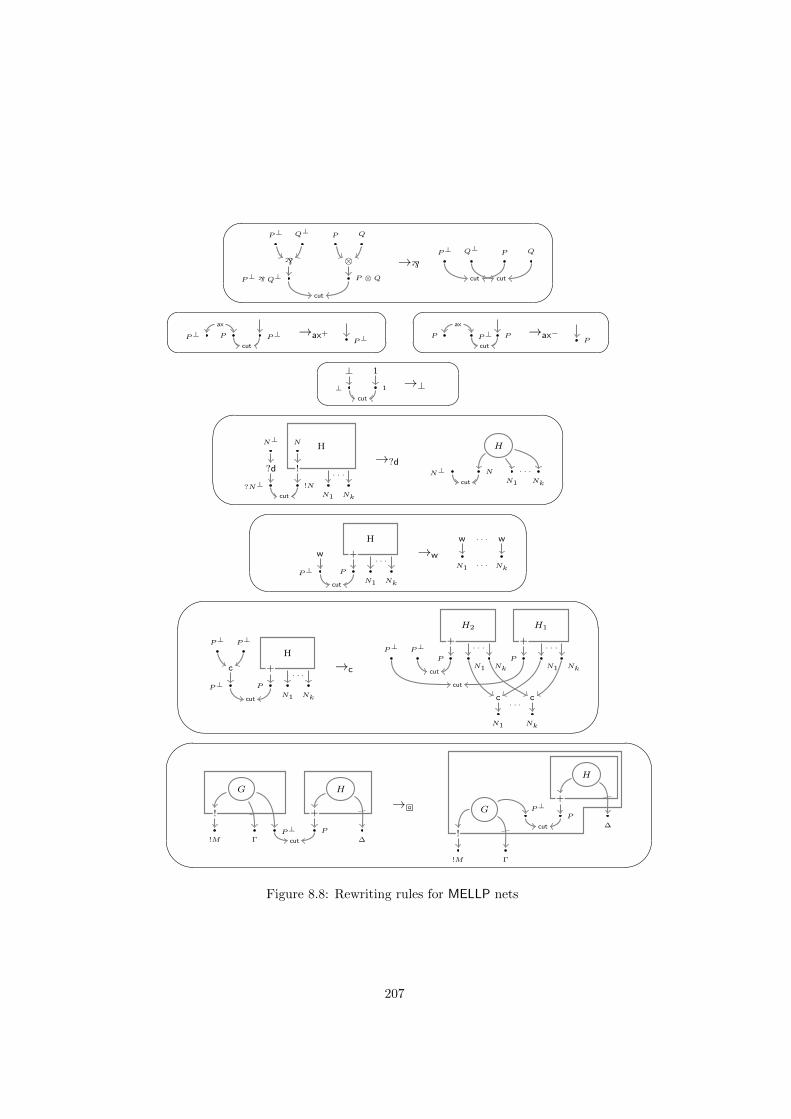
P ⊗ Q

P Q

⊗

P⊥ ` Q⊥

P⊥ Q⊥

`

cut

→`P QQ⊥P⊥

cut cut

P⊥PP⊥

ax

cut

→ax+P⊥

PP⊥P

ax

cut

→ax−P

1

1

⊥

⊥

cut

→⊥

!N

N

!

NkN1

. . .

H

?N⊥

N⊥

?d

cut

→?d

H

N

N1 Nk

. . .N⊥

cut

P⊥

w

P

+

NkN1

H

. . .

cut

→wN1 Nk

w w. . .

. . .

'

&

$

%P⊥

P⊥ P⊥

c

P

+

H

NkN1

. . .

cut

→c

P⊥ P⊥

P

+

H2

NkN1

. . .

cut

P

+

H1

NkN1

. . .

N1 Nk

. . .c c

cut

'

&

$

%!M

!

Γ

G

P⊥ P

+

∆

H

cut

→

!M

!

Γ

G P⊥P

+

∆

H

cut

Figure 8.8: Rewriting rules for MELLP nets

207

'

&

$

%

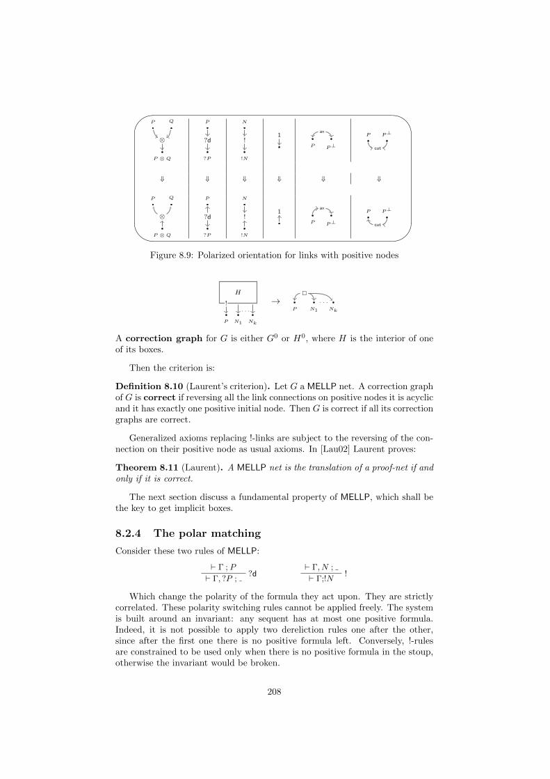
P ⊗ Q

P Q

⊗

P

?P

?d

N

!N

!1

P P⊥

axP P⊥

cut

⇓ ⇓ ⇓ ⇓ ⇓ ⇓

P ⊗ Q

P Q

⊗

P

?P

?d

N

!N

!1

P P⊥

axP P⊥

cut

Figure 8.9: Polarized orientation for links with positive nodes

P

!

NkN1

H

. . .

→NkN1P

. . .

A correction graph for G is either G0 or H0, where H is the interior of oneof its boxes.

Then the criterion is:

Definition 8.10 (Laurent’s criterion). Let G a MELLP net. A correction graphof G is correct if reversing all the link connections on positive nodes it is acyclicand it has exactly one positive initial node. Then G is correct if all its correctiongraphs are correct.

Generalized axioms replacing !-links are subject to the reversing of the con-nection on their positive node as usual axioms. In [Lau02] Laurent proves:

Theorem 8.11 (Laurent). A MELLP net is the translation of a proof-net if andonly if it is correct.

The next section discuss a fundamental property of MELLP, which shall bethe key to get implicit boxes.

8.2.4 The polar matching

Consider these two rules of MELLP:

` Γ ; P?d` Γ, ?P ;

` Γ, N ;!` Γ;!N

Which change the polarity of the formula they act upon. They are strictlycorrelated. These polarity switching rules cannot be applied freely. The systemis built around an invariant: any sequent has at most one positive formula.Indeed, it is not possible to apply two dereliction rules one after the other,since after the first one there is no positive formula left. Conversely, !-rulesare constrained to be used only when there is no positive formula in the stoup,otherwise the invariant would be broken.

208

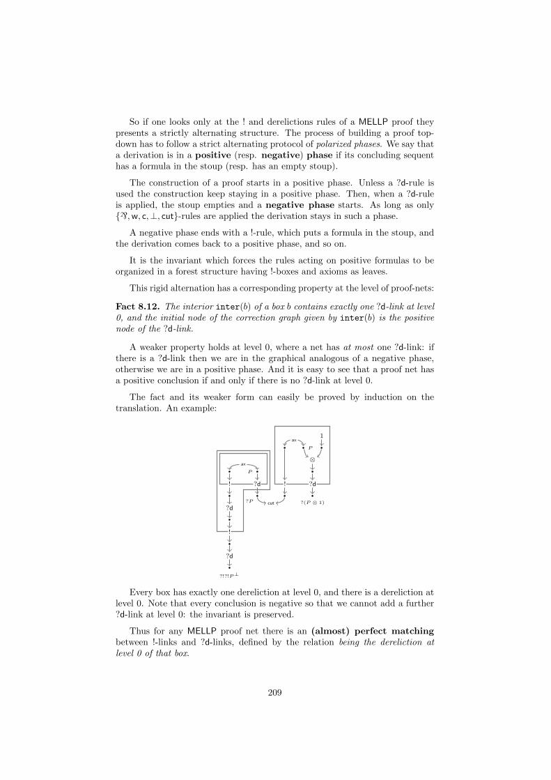
So if one looks only at the ! and derelictions rules of a MELLP proof theypresents a strictly alternating structure. The process of building a proof top-down has to follow a strict alternating protocol of polarized phases. We say thata derivation is in a positive (resp. negative) phase if its concluding sequenthas a formula in the stoup (resp. has an empty stoup).

The construction of a proof starts in a positive phase. Unless a ?d-rule isused the construction keep staying in a positive phase. Then, when a ?d-ruleis applied, the stoup empties and a negative phase starts. As long as only`,w, c,⊥, cut-rules are applied the derivation stays in such a phase.

A negative phase ends with a !-rule, which puts a formula in the stoup, andthe derivation comes back to a positive phase, and so on.

It is the invariant which forces the rules acting on positive formulas to beorganized in a forest structure having !-boxes and axioms as leaves.

This rigid alternation has a corresponding property at the level of proof-nets:

Fact 8.12. The interior inter(b) of a box b contains exactly one ?d-link at level0, and the initial node of the correction graph given by inter(b) is the positivenode of the ?d-link.

A weaker property holds at level 0, where a net has at most one ?d-link: ifthere is a ?d-link then we are in the graphical analogous of a negative phase,otherwise we are in a positive phase. And it is easy to see that a proof net hasa positive conclusion if and only if there is no ?d-link at level 0.

The fact and its weaker form can easily be proved by induction on thetranslation. An example:

P

ax

?P

! ?d

!

?dcut ?(P ⊗ 1)

?d

P

⊗

1ax

!

?!?!P⊥

?d

Every box has exactly one dereliction at level 0, and there is a dereliction atlevel 0. Note that every conclusion is negative so that we cannot add a further?d-link at level 0: the invariant is preserved.

Thus for any MELLP proof net there is an (almost) perfect matchingbetween !-links and ?d-links, defined by the relation being the dereliction atlevel 0 of that box.

209

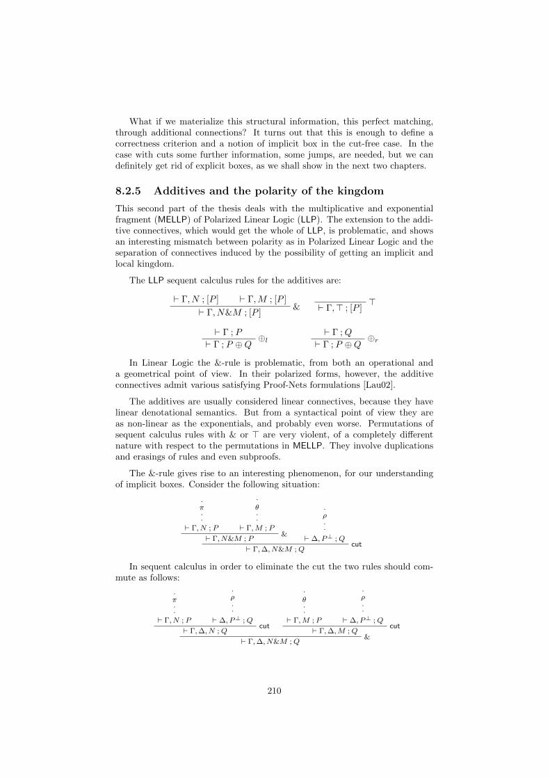
What if we materialize this structural information, this perfect matching,through additional connections? It turns out that this is enough to define acorrectness criterion and a notion of implicit box in the cut-free case. In thecase with cuts some further information, some jumps, are needed, but we candefinitely get rid of explicit boxes, as we shall show in the next two chapters.

8.2.5 Additives and the polarity of the kingdom

This second part of the thesis deals with the multiplicative and exponentialfragment (MELLP) of Polarized Linear Logic (LLP). The extension to the addi-tive connectives, which would get the whole of LLP, is problematic, and showsan interesting mismatch between polarity as in Polarized Linear Logic and theseparation of connectives induced by the possibility of getting an implicit andlocal kingdom.

The LLP sequent calculus rules for the additives are:

` Γ, N ; [P ] ` Γ,M ; [P ]&` Γ, N&M ; [P ]

>` Γ,> ; [P ]

` Γ ; P ⊕l` Γ ; P ⊕Q` Γ ;Q ⊕r` Γ ; P ⊕Q

In Linear Logic the &-rule is problematic, from both an operational anda geometrical point of view. In their polarized forms, however, the additiveconnectives admit various satisfying Proof-Nets formulations [Lau02].

The additives are usually considered linear connectives, because they havelinear denotational semantics. But from a syntactical point of view they areas non-linear as the exponentials, and probably even worse. Permutations ofsequent calculus rules with & or > are very violent, of a completely differentnature with respect to the permutations in MELLP. They involve duplicationsand erasings of rules and even subproofs.

The &-rule gives rise to an interesting phenomenon, for our understandingof implicit boxes. Consider the following situation:

.π..

` Γ, N ; P

.

θ..

` Γ,M ; P&` Γ, N&M ; P

.ρ..

` ∆, P⊥ ;Qcut

` Γ,∆, N&M ;Q

In sequent calculus in order to eliminate the cut the two rules should com-mute as follows:

.π..

` Γ, N ; P

.ρ..

` ∆, P⊥ ;Qcut

` Γ,∆, N ;Q

.

θ..

` Γ,M ; P

.ρ..

` ∆, P⊥ ;Qcut

` Γ,∆,M ;Q&` Γ,∆, N&M ;Q

210

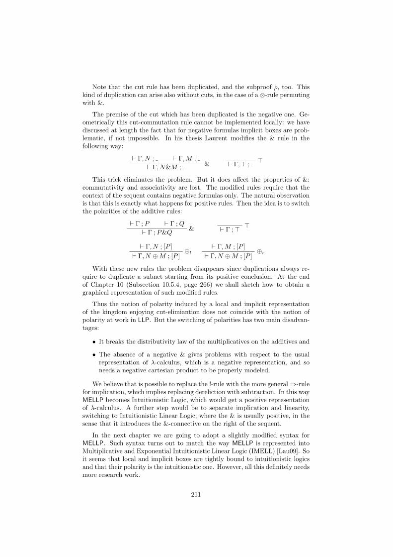
Note that the cut rule has been duplicated, and the subproof ρ, too. Thiskind of duplication can arise also without cuts, in the case of a ⊗-rule permutingwith &.

The premise of the cut which has been duplicated is the negative one. Ge-ometrically this cut-commutation rule cannot be implemented locally: we havediscussed at length the fact that for negative formulas implicit boxes are prob-lematic, if not impossible. In his thesis Laurent modifies the & rule in thefollowing way:

` Γ, N ; ` Γ,M ;&` Γ, N&M ;

>` Γ,> ;

This trick eliminates the problem. But it does affect the properties of &:commutativity and associativity are lost. The modified rules require that thecontext of the sequent contains negative formulas only. The natural observationis that this is exactly what happens for positive rules. Then the idea is to switchthe polarities of the additive rules:

` Γ ; P ` Γ ;Q&` Γ ; P&Q

>` Γ ;>

` Γ, N ; [P ]⊕l` Γ, N ⊕M ; [P ]

` Γ,M ; [P ]⊕r` Γ, N ⊕M ; [P ]

With these new rules the problem disappears since duplications always re-quire to duplicate a subnet starting from its positive conclusion. At the endof Chapter 10 (Subsection 10.5.4, page 266) we shall sketch how to obtain agraphical representation of such modified rules.

Thus the notion of polarity induced by a local and implicit representationof the kingdom enjoying cut-elimiantion does not coincide with the notion ofpolarity at work in LLP. But the switching of polarities has two main disadvan-tages:

• It breaks the distributivity law of the multiplicatives on the additives and

• The absence of a negative & gives problems with respect to the usualrepresentation of λ-calculus, which is a negative representation, and soneeds a negative cartesian product to be properly modeled.

We believe that is possible to replace the !-rule with the more general⇒-rulefor implication, which implies replacing dereliction with subtraction. In this wayMELLP becomes Intuitionistic Logic, which would get a positive representationof λ-calculus. A further step would be to separate implication and linearity,switching to Intuitionistic Linear Logic, where the & is usually positive, in thesense that it introduces the &-connective on the right of the sequent.

In the next chapter we are going to adopt a slightly modified syntax forMELLP. Such syntax turns out to match the way MELLP is represented intoMultiplicative and Exponential Intuitionistic Linear Logic (IMELL) [Lau09]. Soit seems that local and implicit boxes are tightly bound to intuitionistic logicsand that their polarity is the intuitionistic one. However, all this definitely needsmore research work.

211

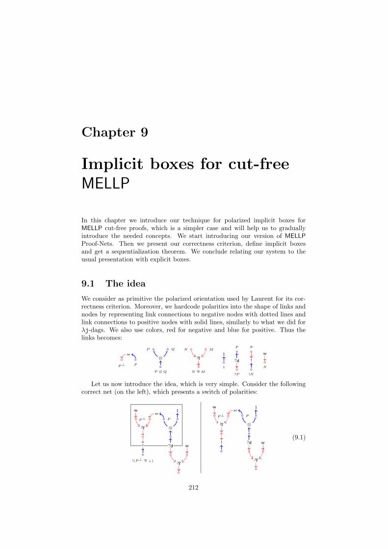
Chapter 9

Implicit boxes for cut-freeMELLP

In this chapter we introduce our technique for polarized implicit boxes forMELLP cut-free proofs, which is a simpler case and will help us to graduallyintroduce the needed concepts. We start introducing our version of MELLPProof-Nets. Then we present our correctness criterion, define implicit boxesand get a sequentialization theorem. We conclude relating our system to theusual presentation with explicit boxes.

9.1 The idea

We consider as primitive the polarized orientation used by Laurent for its cor-rectness criterion. Moreover, we hardcode polarities into the shape of links andnodes by representing link connections to negative nodes with dotted lines andlink connections to positive nodes with solid lines, similarly to what we did forλj-dags. We also use colors, red for negative and blue for positive. Thus thelinks becomes:

P⊥ P

ax

P ⊗ Q

P Q

⊗

N `M

N M

`

1

1

?P

P

?d

!N

N

!

N

w

Let us now introduce the idea, which is very simple. Consider the followingcorrect net (on the left), which presents a switch of polarities:

P⊥ P

ax1w

` ⊗

?d w

`!(P⊥ ` ⊥)

!

P⊥ P

ax1w

` ⊗

?d! w

`

(9.1)

212

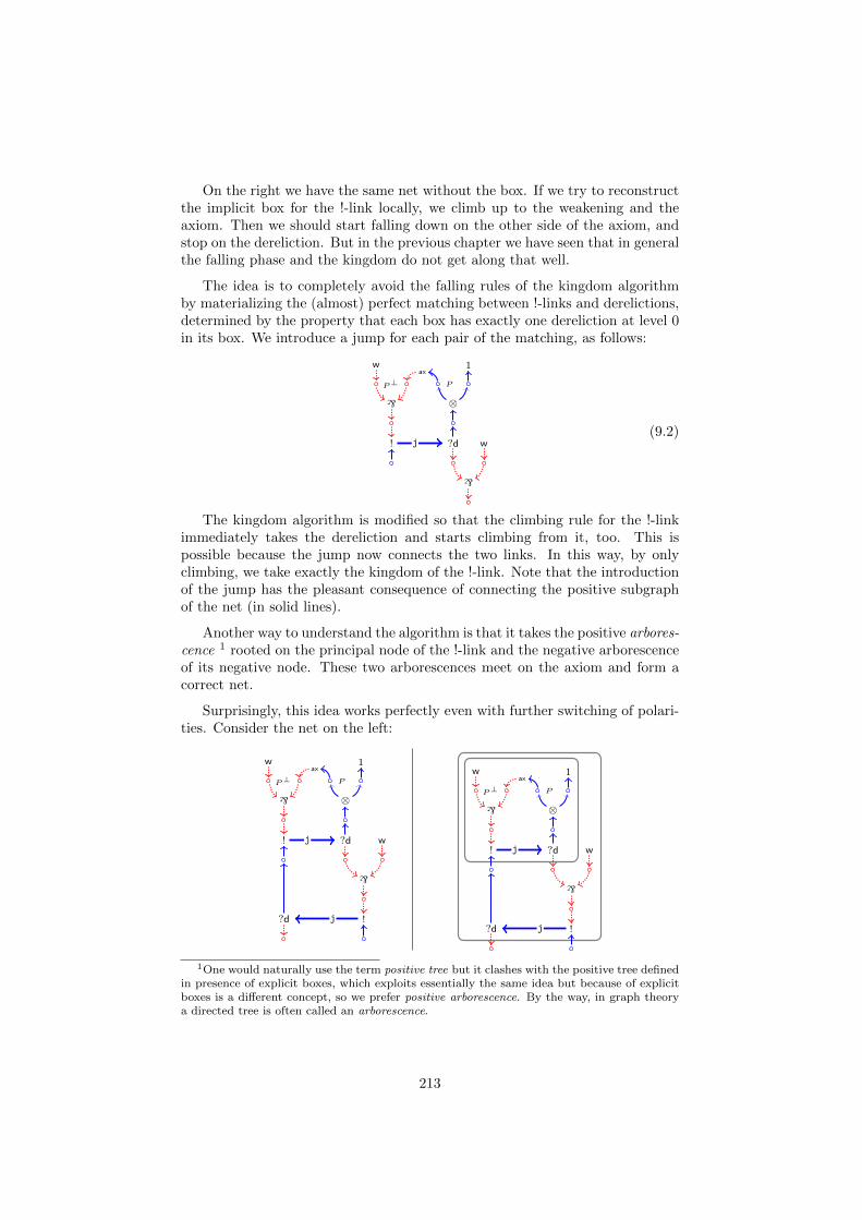
On the right we have the same net without the box. If we try to reconstructthe implicit box for the !-link locally, we climb up to the weakening and theaxiom. Then we should start falling down on the other side of the axiom, andstop on the dereliction. But in the previous chapter we have seen that in generalthe falling phase and the kingdom do not get along that well.

The idea is to completely avoid the falling rules of the kingdom algorithmby materializing the (almost) perfect matching between !-links and derelictions,determined by the property that each box has exactly one dereliction at level 0in its box. We introduce a jump for each pair of the matching, as follows:

P⊥ P

ax1w

` ⊗

?d! w

`

j(9.2)

The kingdom algorithm is modified so that the climbing rule for the !-linkimmediately takes the dereliction and starts climbing from it, too. This ispossible because the jump now connects the two links. In this way, by onlyclimbing, we take exactly the kingdom of the !-link. Note that the introductionof the jump has the pleasant consequence of connecting the positive subgraphof the net (in solid lines).

Another way to understand the algorithm is that it takes the positive arbores-cence 1 rooted on the principal node of the !-link and the negative arborescenceof its negative node. These two arborescences meet on the axiom and form acorrect net.

Surprisingly, this idea works perfectly even with further switching of polari-ties. Consider the net on the left:

P⊥ P

ax1w

` ⊗

?d! j w

`

!?d j

P⊥ P

ax1w

` ⊗

?d! j w

`

!?d j

1One would naturally use the term positive tree but it clashes with the positive tree definedin presence of explicit boxes, which exploits essentially the same idea but because of explicitboxes is a different concept, so we prefer positive arborescence. By the way, in graph theorya directed tree is often called an arborescence.

213

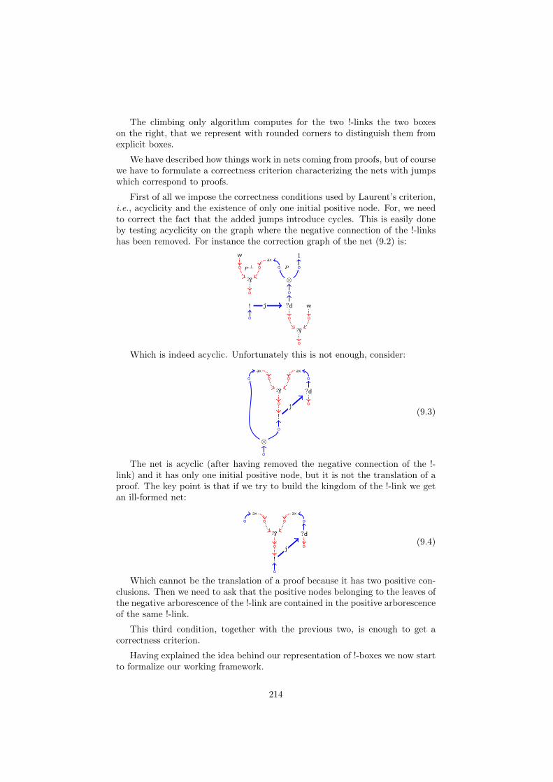
The climbing only algorithm computes for the two !-links the two boxeson the right, that we represent with rounded corners to distinguish them fromexplicit boxes.

We have described how things work in nets coming from proofs, but of coursewe have to formulate a correctness criterion characterizing the nets with jumpswhich correspond to proofs.

First of all we impose the correctness conditions used by Laurent’s criterion,i.e., acyclicity and the existence of only one initial positive node. For, we needto correct the fact that the added jumps introduce cycles. This is easily doneby testing acyclicity on the graph where the negative connection of the !-linkshas been removed. For instance the correction graph of the net (9.2) is:

P⊥ P

ax1w

` ⊗

?d! w

`

j

Which is indeed acyclic. Unfortunately this is not enough, consider:

axax

` ?d

!

j

⊗

(9.3)

The net is acyclic (after having removed the negative connection of the !-link) and it has only one initial positive node, but it is not the translation of aproof. The key point is that if we try to build the kingdom of the !-link we getan ill-formed net:

axax

` ?d

!

j(9.4)

Which cannot be the translation of a proof because it has two positive con-clusions. Then we need to ask that the positive nodes belonging to the leaves ofthe negative arborescence of the !-link are contained in the positive arborescenceof the same !-link.

This third condition, together with the previous two, is enough to get acorrectness criterion.

Having explained the idea behind our representation of !-boxes we now startto formalize our working framework.

214

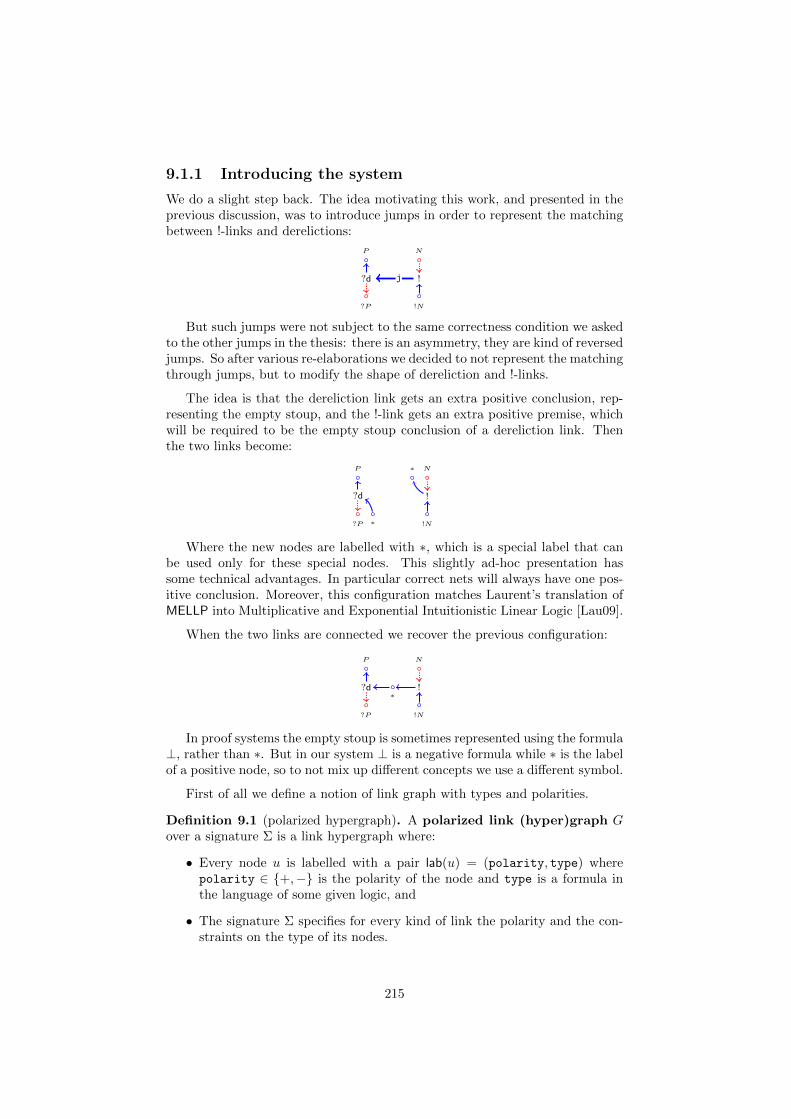
9.1.1 Introducing the system

We do a slight step back. The idea motivating this work, and presented in theprevious discussion, was to introduce jumps in order to represent the matchingbetween !-links and derelictions:

?P

P

?d

!N

N

!j

But such jumps were not subject to the same correctness condition we askedto the other jumps in the thesis: there is an asymmetry, they are kind of reversedjumps. So after various re-elaborations we decided to not represent the matchingthrough jumps, but to modify the shape of dereliction and !-links.

The idea is that the dereliction link gets an extra positive conclusion, rep-resenting the empty stoup, and the !-link gets an extra positive premise, whichwill be required to be the empty stoup conclusion of a dereliction link. Thenthe two links become:

?P

P

∗

?d

!N

N∗

!

Where the new nodes are labelled with ∗, which is a special label that canbe used only for these special nodes. This slightly ad-hoc presentation hassome technical advantages. In particular correct nets will always have one pos-itive conclusion. Moreover, this configuration matches Laurent’s translation ofMELLP into Multiplicative and Exponential Intuitionistic Linear Logic [Lau09].

When the two links are connected we recover the previous configuration:

?P

P

?d

!N

N

!∗

In proof systems the empty stoup is sometimes represented using the formula⊥, rather than ∗. But in our system ⊥ is a negative formula while ∗ is the labelof a positive node, so to not mix up different concepts we use a different symbol.

First of all we define a notion of link graph with types and polarities.

Definition 9.1 (polarized hypergraph). A polarized link (hyper)graph Gover a signature Σ is a link hypergraph where:

• Every node u is labelled with a pair lab(u) = (polarity, type) wherepolarity ∈ +,− is the polarity of the node and type is a formula inthe language of some given logic, and

• The signature Σ specifies for every kind of link the polarity and the con-straints on the type of its nodes.

215

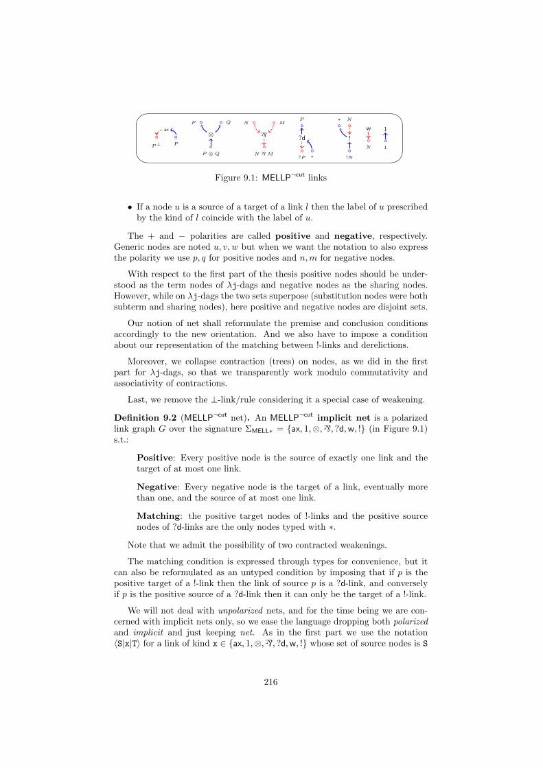
P⊥ P

ax

P ⊗ Q

P Q

⊗

N `M

N M

`

?P

P

∗

?d

!N

N∗

!

N

w

1

1

Figure 9.1: MELLP¬cut links

• If a node u is a source of a target of a link l then the label of u prescribedby the kind of l coincide with the label of u.

The + and − polarities are called positive and negative, respectively.Generic nodes are noted u, v, w but when we want the notation to also expressthe polarity we use p, q for positive nodes and n,m for negative nodes.

With respect to the first part of the thesis positive nodes should be under-stood as the term nodes of λj-dags and negative nodes as the sharing nodes.However, while on λj-dags the two sets superpose (substitution nodes were bothsubterm and sharing nodes), here positive and negative nodes are disjoint sets.

Our notion of net shall reformulate the premise and conclusion conditionsaccordingly to the new orientation. And we also have to impose a conditionabout our representation of the matching between !-links and derelictions.

Moreover, we collapse contraction (trees) on nodes, as we did in the firstpart for λj-dags, so that we transparently work modulo commutativity andassociativity of contractions.

Last, we remove the ⊥-link/rule considering it a special case of weakening.

Definition 9.2 (MELLP¬cut net). An MELLP¬cut implicit net is a polarizedlink graph G over the signature ΣMELL∗ = ax, 1,⊗,`, ?d,w, ! (in Figure 9.1)s.t.:

Positive: Every positive node is the source of exactly one link and thetarget of at most one link.

Negative: Every negative node is the target of a link, eventually morethan one, and the source of at most one link.

Matching: the positive target nodes of !-links and the positive sourcenodes of ?d-links are the only nodes typed with ∗.

Note that we admit the possibility of two contracted weakenings.

The matching condition is expressed through types for convenience, but itcan also be reformulated as an untyped condition by imposing that if p is thepositive target of a !-link then the link of source p is a ?d-link, and converselyif p is the positive source of a ?d-link then it can only be the target of a !-link.

We will not deal with unpolarized nets, and for the time being we are con-cerned with implicit nets only, so we ease the language dropping both polarizedand implicit and just keeping net. As in the first part we use the notation〈S|x|T〉 for a link of kind x ∈ ax, 1,⊗,`, ?d,w, ! whose set of source nodes is S

216

'

&

$

%

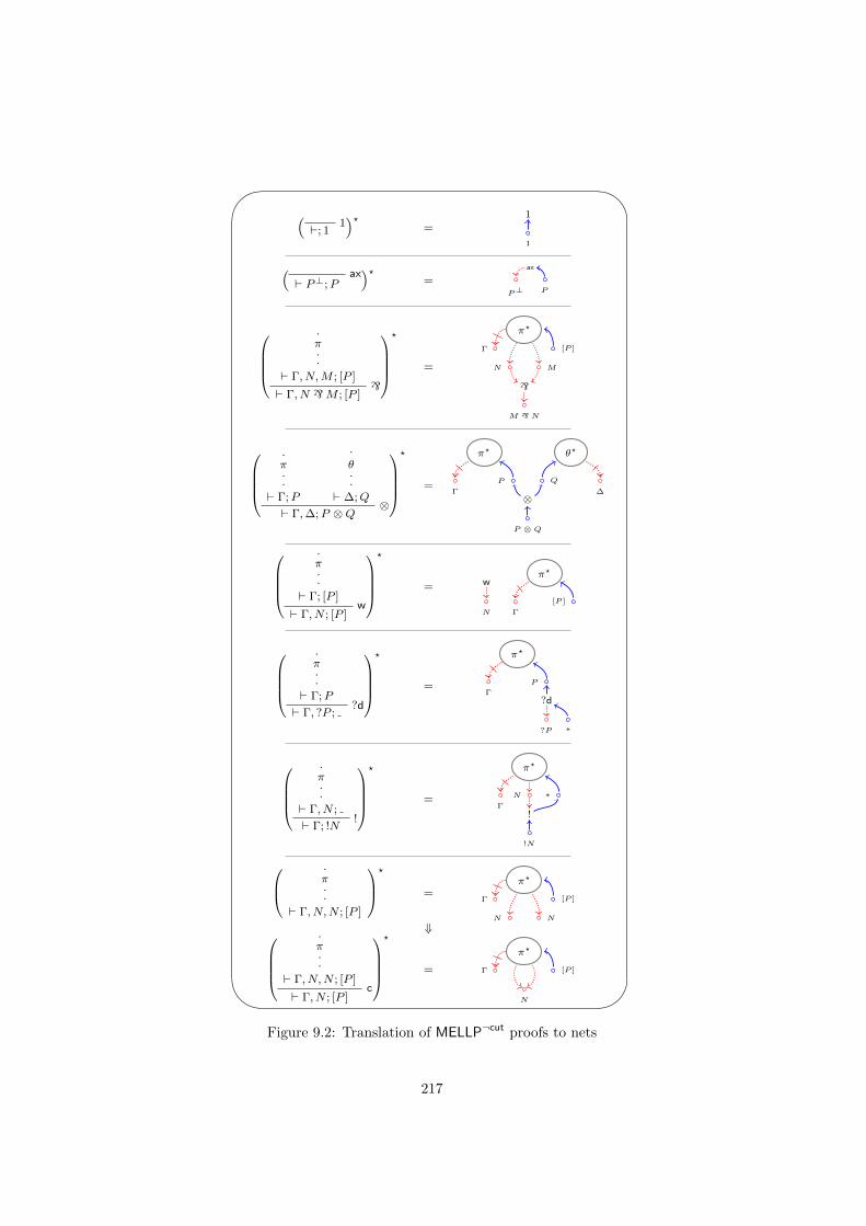
(1`; 1

)?=

1

1

(ax

` P⊥;P

)?=

P⊥ P

ax

.π..

` Γ, N,M ; [P ]`` Γ, N `M ; [P ]

?

=

π?

MN

Γ [P ]

M ` N

`

.π..

` Γ;P

.

θ..

` ∆;Q⊗

` Γ,∆;P ⊗Q

?

=

π?

Γ

P

θ?

∆

Q

P ⊗ Q

⊗

.π..

` Γ; [P ]w

` Γ, N ; [P ]

?

=π?

Γ

[P ]

N

w

.π..

` Γ;P?d` Γ, ?P ;

?

=

π?

Γ

P

?P ∗

?d

.π..

` Γ, N ;!` Γ; !N

?

=

π?

Γ

∗N

!N

!

.π..

` Γ, N,N ; [P ]

?

=π?

NN

Γ [P ]

⇓.π..

` Γ, N,N ; [P ]c

` Γ, N ; [P ]

?

=

π?

N

Γ [P ]

Figure 9.2: Translation of MELLP¬cut proofs to nets

217

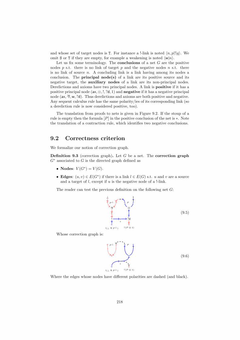
and whose set of target nodes is T. For instance a !-link is noted 〈n, p|!|q〉. Weomit S or T if they are empty, for example a weakening is noted 〈w|n〉.

Let us fix some terminology. The conclusions of a net G are the positivenodes p s.t. there is no link of target p and the negative nodes n s.t. thereis no link of source n. A concluding link is a link having among its nodes aconclusion. The principal node(s) of a link are its positive source and itsnegative target, the auxiliary nodes of a link are its non-principal nodes.Derelictions and axioms have two principal nodes. A link is positive if it has apositive principal node (ax,⊗, !, ?d, 1) and negative if it has a negative principalnode (ax,`,w, ?d). Thus derelictions and axioms are both positive and negative.Any sequent calculus rule has the same polarity/ies of its corresponding link (soa dereliction rule is now considered positive, too).

The translation from proofs to nets is given in Figure 9.2. If the stoup of arule is empty then the formula [P ] in the positive conclusion of the net is ∗. Notethe translation of a contraction rule, which identifies two negative conclusions.

9.2 Correctness criterion

We formalize our notion of correction graph.

Definition 9.3 (correction graph). Let G be a net. The correction graphG∗ associated to G is the directed graph defined as

• Nodes: V (G∗) = V (G).

• Edges: (u, v) ∈ E(G∗) if there is a link l ∈ E(G) s.t. u and v are a sourceand a target of l, except if u is the negative node of a !-link.

The reader can test the previous definition on the following net G:

P⊥ P

ax1⊥

` ⊗

?(P ⊗ 1)

∗?d

!(⊥ ` P⊥)

!

(9.5)

Whose correction graph is:

P⊥ P

?(P ⊗ 1)

∗

!(⊥ ` P⊥)

(9.6)

Where the edges whose nodes have different polarities are dashed (and black).

218

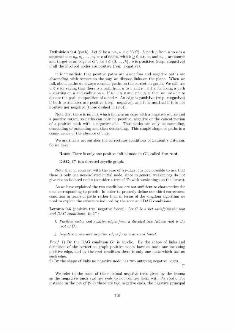
Definition 9.4 (path). Let G be a net, u, v ∈ V (G). A path ρ from u to v is asequence u = u0, u1, . . . , uk = v of nodes, with k ≥ 0, s.t. ui and ui+1 are sourceand target of an edge of G∗, for i ∈ 0, . . . , k. ρ is positive (resp. negative)if all the involved nodes are positive (resp. negative).

It is immediate that positive paths are ascending and negative paths aredescending, with respect to the way we dispose links on the plane. When wetalk about paths we always consider paths on the correction graph. We still useu 6 v for saying that there is a path from u to v and ν : u 6 v for fixing a pathν starting on u and ending on v. If ν : u 6 v and τ : v 6 w then we use ν ; τ todenote the path composition of ν and τ . An edge is positive (resp. negative)if both extremities are positive (resp. negative), and it is neutral if it is notpositive nor negative (those dashed in (9.6)).

Note that there is no link which induces an edge with a negative source anda positive target, so paths can only be positive, negative or the concatenationof a positive path with a negative one. Thus paths can only be ascending,descending or ascending and then descending. This simple shape of paths is aconsequence of the absence of cuts.

We ask that a net satisfies the correctness conditions of Laurent’s criterion.So we have:

Root: There is only one positive initial node in G∗, called the root.

DAG: G∗ is a directed acyclic graph.

Note that in contrast with the case of λj-dags it is not possible to ask thatthere is only one non-isolated initial node, since in general weakenings do notgive rise to isolated nodes (consider a tree of `s with weakenings on the leaves).

As we have explained the two conditions are not sufficient to characterize thenets corresponding to proofs. In order to properly define our third correctnesscondition in terms of paths rather than in terms of the kingdom algorithm weneed to exploit the structure induced by the root and DAG conditions.

Lemma 9.5 (positive tree, negative forest). Let G be a net satisfying the rootand DAG conditions. In G∗:

1. Positive nodes and positive edges form a directed tree (whose root is theroot of G).

2. Negative nodes and negative edges form a directed forest.

Proof. 1) By the DAG condition G∗ is acyclic. By the shape of links anddefinition of the correction graph positive nodes have at most one incomingpositive edge, and by the root condition there is only one node which has nosuch edge.2) By the shape of links no negative node has two outgoing negative edges.

We refer to the roots of the maximal negative trees given by the lemmaas the negative ends (we use ends to not confuse them with the root). Forinstance in the net of (9.5) there are two negative ends, the negative principal

219

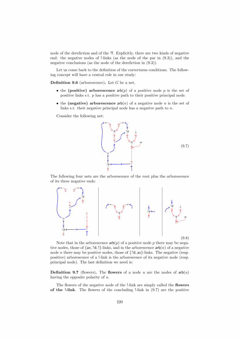
node of the dereliction and of the `. Explicitly, there are two kinds of negativeend: the negative nodes of !-links (as the node of the par in (9.3)), and thenegative conclusions (as the node of the dereliction in (9.3)).

Let us come back to the definition of the correctness conditions. The follow-ing concept will have a central role in our study:

Definition 9.6 (arborescence). Let G be a net.

• the (positive) arborescence arb(p) of a positive node p is the set ofpositive links s.t. p has a positive path to their positive principal node.

• the (negative) arborescence arb(n) of a negative node n is the set oflinks s.t. their negative principal node has a negative path to n.

Consider the following net:

axax

` ?d

!

⊗

⊥

` w

!?d

(9.7)

The following four nets are the arborescence of the root plus the arborescenceof its three negative ends:

axax

?d

!

⊗

!?d

axax

` ?d

?d ⊥

` w

(9.8)Note that in the arborescence arb(p) of a positive node p there may be nega-

tive nodes, those of ax, ?d, !-links, and in the arborescence arb(n) of a negativenode n there may be positive nodes, those of ?d, ax-links. The negative (resp.positive) arborescence of a !-link is the arborescence of its negative node (resp.principal node). The last definition we need is:

Definition 9.7 (flowers). The flowers of a node u are the nodes of arb(u)having the opposite polarity of u.

The flowers of the negative node of the !-link are simply called the flowersof the !-link. The flowers of the concluding !-link in (9.7) are the positive

220

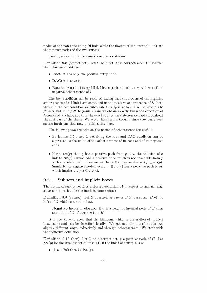
nodes of the non-concluding ?d-link, while the flowers of the internal !-link arethe positive nodes of the two axioms.

Finally, we can formulate our correctness criterion:

Definition 9.8 (correct net). Let G be a net. G is correct when G∗ satisfiesthe following conditions:

• Root: it has only one positive entry node.

• DAG: it is acyclic.

• Box: the ∗-node of every !-link l has a positive path to every flower of thenegative arborescence of l.

The box condition can be restated saying that the flowers of the negativearborescence of a !-link l are contained in the positive arborescence of l. Notethat if in the box condition we substitute binding node to ∗ node, occurrences toflowers and solid path to positive path we obtain exactly the scope condition ofλ-trees and λj-dags, and thus the exact copy of the criterion we used throughoutthe first part of the thesis. We avoid those terms, though, since they carry verystrong intuitions that may be misleading here.

The following two remarks on the notion of arborescence are useful:

• By lemma 9.5 a net G satisfying the root and DAG condition can beexpressed as the union of the arborescences of its root and of its negativeends.

• If q ∈ arb(p) then q has a positive path from p, i.e., the addition of alink to arb(p) cannot add a positive node which is not reachable from pwith a positive path. Then we get that q ∈ arb(p) implies arb(q) ⊆ arb(p).Similarly, for negative nodes: every m ∈ arb(n) has a negative path to m,which implies arb(m) ⊆ arb(n).

9.2.1 Subnets and implicit boxes

The notion of subnet requires a closure condition with respect to internal neg-ative nodes, to handle the implicit contractions:

Definition 9.9 (subnet). Let G be a net. A subnet of G is a subset H of thelinks of G which is a net and s.t.

Negative internal closure: if n is a negative internal node of H thenany link l of G of target n is in H.

It is now time to show that the kingdom, which is our notion of implicitbox, exists and can be described locally. We can actually describe it in twoslightly different ways, inductively and through arborescences. We start withthe inductive definition.

Definition 9.10 (box). Let G be a correct net, p a positive node of G. Letbox(p) be the smallest set of links s.t. if the link l of source p is a:

• 1, ax-link then l ∈ box(p).

221

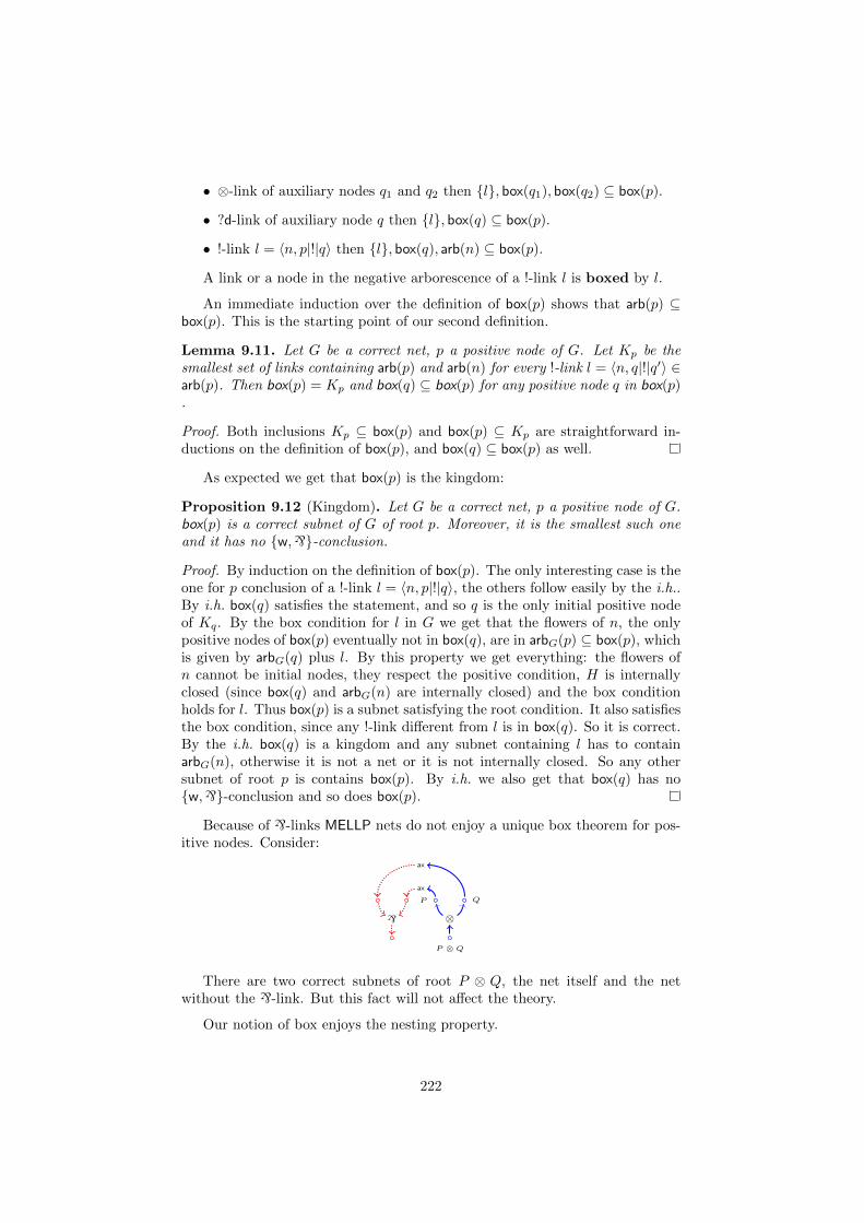
• ⊗-link of auxiliary nodes q1 and q2 then l, box(q1), box(q2) ⊆ box(p).

• ?d-link of auxiliary node q then l, box(q) ⊆ box(p).

• !-link l = 〈n, p|!|q〉 then l, box(q), arb(n) ⊆ box(p).

A link or a node in the negative arborescence of a !-link l is boxed by l.

An immediate induction over the definition of box(p) shows that arb(p) ⊆box(p). This is the starting point of our second definition.

Lemma 9.11. Let G be a correct net, p a positive node of G. Let Kp be thesmallest set of links containing arb(p) and arb(n) for every !-link l = 〈n, q|!|q′〉 ∈arb(p). Then box(p) = Kp and box(q) ⊆ box(p) for any positive node q in box(p).

Proof. Both inclusions Kp ⊆ box(p) and box(p) ⊆ Kp are straightforward in-ductions on the definition of box(p), and box(q) ⊆ box(p) as well.

As expected we get that box(p) is the kingdom:

Proposition 9.12 (Kingdom). Let G be a correct net, p a positive node of G.box(p) is a correct subnet of G of root p. Moreover, it is the smallest such oneand it has no w,`-conclusion.

Proof. By induction on the definition of box(p). The only interesting case is theone for p conclusion of a !-link l = 〈n, p|!|q〉, the others follow easily by the i.h..By i.h. box(q) satisfies the statement, and so q is the only initial positive nodeof Kq. By the box condition for l in G we get that the flowers of n, the onlypositive nodes of box(p) eventually not in box(q), are in arbG(p) ⊆ box(p), whichis given by arbG(q) plus l. By this property we get everything: the flowers ofn cannot be initial nodes, they respect the positive condition, H is internallyclosed (since box(q) and arbG(n) are internally closed) and the box conditionholds for l. Thus box(p) is a subnet satisfying the root condition. It also satisfiesthe box condition, since any !-link different from l is in box(q). So it is correct.By the i.h. box(q) is a kingdom and any subnet containing l has to containarbG(n), otherwise it is not a net or it is not internally closed. So any othersubnet of root p is contains box(p). By i.h. we also get that box(q) has now,`-conclusion and so does box(p).

Because of `-links MELLP nets do not enjoy a unique box theorem for pos-itive nodes. Consider:

P ⊗ Q

P Q

⊗`

ax

ax

There are two correct subnets of root P ⊗ Q, the net itself and the netwithout the `-link. But this fact will not affect the theory.

Our notion of box enjoys the nesting property.

222

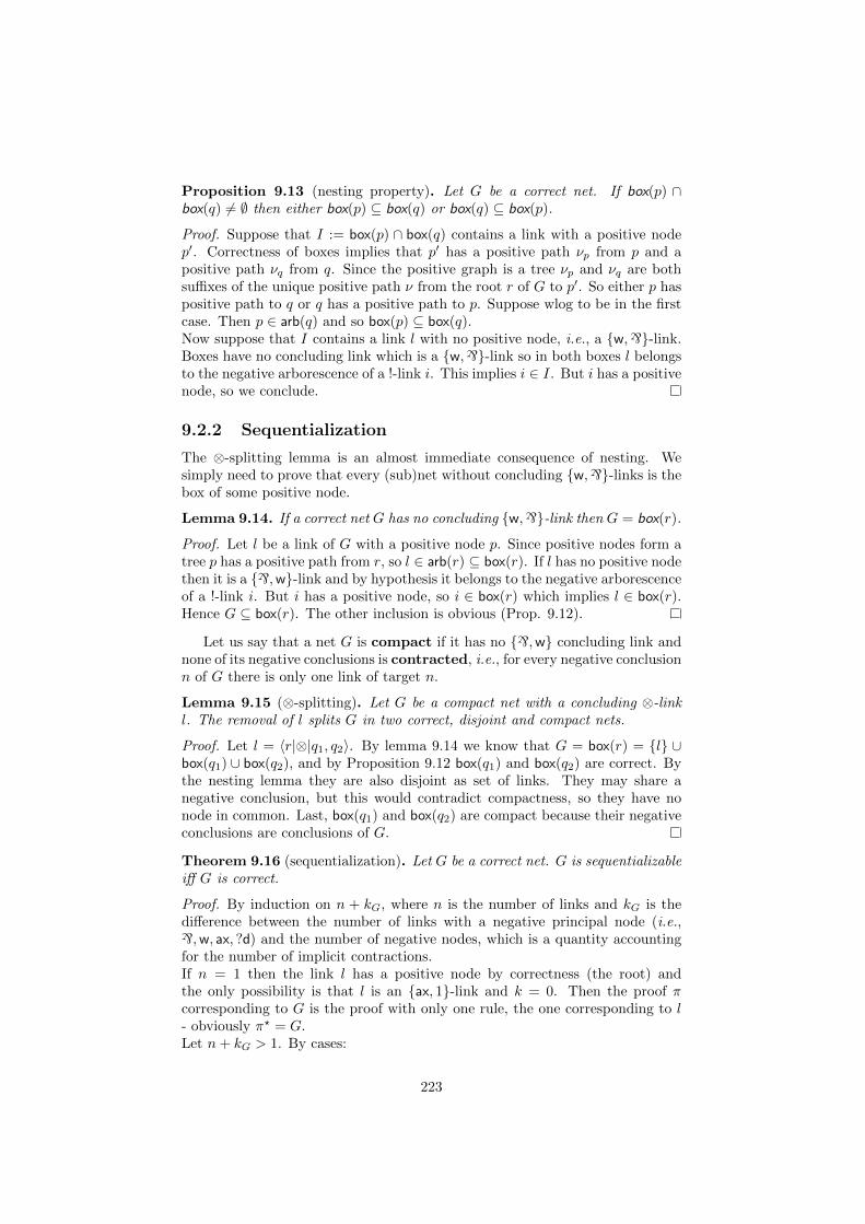
Proposition 9.13 (nesting property). Let G be a correct net. If box(p) ∩box(q) 6= ∅ then either box(p) ⊆ box(q) or box(q) ⊆ box(p).

Proof. Suppose that I := box(p) ∩ box(q) contains a link with a positive nodep′. Correctness of boxes implies that p′ has a positive path νp from p and apositive path νq from q. Since the positive graph is a tree νp and νq are bothsuffixes of the unique positive path ν from the root r of G to p′. So either p haspositive path to q or q has a positive path to p. Suppose wlog to be in the firstcase. Then p ∈ arb(q) and so box(p) ⊆ box(q).Now suppose that I contains a link l with no positive node, i.e., a w,`-link.Boxes have no concluding link which is a w,`-link so in both boxes l belongsto the negative arborescence of a !-link i. This implies i ∈ I. But i has a positivenode, so we conclude.

9.2.2 Sequentialization

The ⊗-splitting lemma is an almost immediate consequence of nesting. Wesimply need to prove that every (sub)net without concluding w,`-links is thebox of some positive node.

Lemma 9.14. If a correct net G has no concluding w,`-link then G = box(r).

Proof. Let l be a link of G with a positive node p. Since positive nodes form atree p has a positive path from r, so l ∈ arb(r) ⊆ box(r). If l has no positive nodethen it is a `,w-link and by hypothesis it belongs to the negative arborescenceof a !-link i. But i has a positive node, so i ∈ box(r) which implies l ∈ box(r).Hence G ⊆ box(r). The other inclusion is obvious (Prop. 9.12).

Let us say that a net G is compact if it has no `,w concluding link andnone of its negative conclusions is contracted, i.e., for every negative conclusionn of G there is only one link of target n.

Lemma 9.15 (⊗-splitting). Let G be a compact net with a concluding ⊗-linkl. The removal of l splits G in two correct, disjoint and compact nets.

Proof. Let l = 〈r|⊗|q1, q2〉. By lemma 9.14 we know that G = box(r) = l ∪box(q1) ∪ box(q2), and by Proposition 9.12 box(q1) and box(q2) are correct. Bythe nesting lemma they are also disjoint as set of links. They may share anegative conclusion, but this would contradict compactness, so they have nonode in common. Last, box(q1) and box(q2) are compact because their negativeconclusions are conclusions of G.

Theorem 9.16 (sequentialization). Let G be a correct net. G is sequentializableiff G is correct.

Proof. By induction on n + kG, where n is the number of links and kG is thedifference between the number of links with a negative principal node (i.e.,`,w, ax, ?d) and the number of negative nodes, which is a quantity accountingfor the number of implicit contractions.If n = 1 then the link l has a positive node by correctness (the root) andthe only possibility is that l is an ax, 1-link and k = 0. Then the proof πcorresponding to G is the proof with only one rule, the one corresponding to l- obviously π? = G.Let n+ kG > 1. By cases:

223

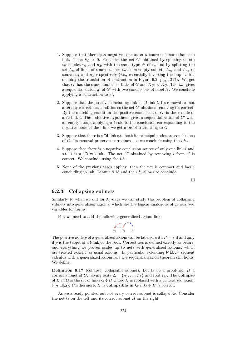
1. Suppose that there is a negative conclusion n source of more than onelink. Then kG > 0. Consider the net G′ obtained by splitting n intotwo nodes n1 and n2, with the same type N of n, and by splitting theset Ln of links of source n into two non-empty subsets Ln1 and Ln2 ofsource n1 and n2 respectively (i.e., essentially inverting the implicationdefining the translation of contraction in Figure 9.2, page 217). We getthat G′ has the same number of links of G and KG′ < KG. The i.h. givesa sequentialization π′ of G′ with two conclusions of label N . We concludeapplying a contraction to π′.

2. Suppose that the positive concluding link is a !-link l. Its removal cannotalter any correctness condition so the net G′ obtained removing l is correct.By the matching condition the positive conclusion of G′ is the ∗ node ofa ?d-link i. The inductive hypothesis gives a sequentialization of G′ withan empty stoup, applying a !-rule to the conclusion corresponding to thenegative node of the !-link we get a proof translating to G.

3. Suppose that there is a ?d-link s.t. both its principal nodes are conclusionsof G. Its removal preserves correctness, so we conclude using the i.h..

4. Suppose that there is a negative conclusion source of only one link l ands.t. l is a `,w-link. The net G′ obtained by removing l from G iscorrect. We conclude using the i.h..

5. None of the previous cases applies: then the net is compact and has aconcluding ⊗-link. Lemma 9.15 and the i.h. allows to conclude.

9.2.3 Collapsing subnets

Similarly to what we did for λj-dags we can study the problem of collapsingsubnets into generalized axioms, which are the logical analogous of generalizedvariables for terms.

For, we need to add the following generalized axiom link:

N1 Nk P

. . .

The positive node p of a generalized axiom can be labeled with P = ∗ if and onlyif p is the target of a !-link or the root. Correctness is defined exactly as before,and everything we proved scales up to nets with generalized axioms, whichare treated exactly as usual axioms. In particular extending MELLP sequentcalculus with a generalized axiom rule the sequentialization theorem still holds.We define:

Definition 9.17 (collapse, collapsible subnet). Let G be a proof-net, H acorrect subnet of G, having exits ∆ = n1, . . . , nk and root rH . The collapseof H in G is the set of links G÷H where H is replaced with a generalized axiom〈rH ||∆〉. Furthermore, H is collapsible in G if G÷H is correct.

As we already pointed out not every correct subnet is collapsible. Considerthe net G on the left and its correct subnet H on the right:

224

⊗

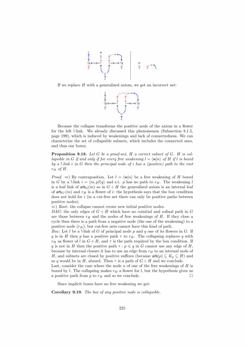
ax

?d!

1 w

?d !ax

w

If we replace H with a generalized axiom, we get an incorrect net:

⊗

ax

?d!

1

?d !

Because the collapse transforms the positive node of the axiom in a flowerfor the left !-link. We already discussed this phenomenon (Subsection 8.1.5,page 199), which is induced by weakenings and lack of connectedness. We cancharacterize the set of collapsible subnets, which includes the connected ones,and thus our boxes.

Proposition 9.18. Let G be a proof-net, H a correct subnet of G. H is col-lapsible in G if and only if for every free weakening l = 〈w|n〉 of H if l is boxedby a !-link i in G then the principal node of i has a (positive) path to the rootrH of H.

Proof. ⇒) By contraposition. Let l = 〈w|n〉 be a free weakening of H boxedin G by a !-link i = 〈m, p|!|q〉 and s.t. p has no path to rH . The weakening lis a leaf link of arbG(m) so in G ÷H the generalized axiom is an internal leafof arbG′(m) and rH is a flower of i: the hypothesis says that the box conditiondoes not hold for i (in a cut-free net there can only be positive paths betweenpositive nodes).⇐) Root : the collapse cannot create new initial positive nodes.DAG : the only edges of G ÷ H which have no coinitial and cofinal path in Gare those between rH and the nodes of free weakenings of H. If they close acycle then there is a path from a negative node (the one of the weakening) to apositive node (rH), but cut-free nets cannot have this kind of path.Box : Let l be a !-link of G of principal node p and q one of its flowers in G. Ifq is in H then p has a positive path τ to rH . The collapsing replaces q withrH as flower of l in G÷H, and τ is the path required by the box condition. Ifq is not in H then the positive path τ : p 6 q in G cannot use any edge of H,because by internal closure it has to use an edge from rH to an internal node ofH, and subnets are closed by positive suffixes (because arb(p) ⊆ Kp ⊆ H) andso q would be in H, absurd. Then τ is a path of G÷H and we conclude.Last, consider the case where the node n of one of the free weakenings of H isboxed by l. The collapsing makes rH a flower for l, but the hypothesis gives usa positive path from p to rH and so we conclude.

Since implicit boxes have no free weakening we get:

Corollary 9.19. The box of any positive node is collapsible.

225

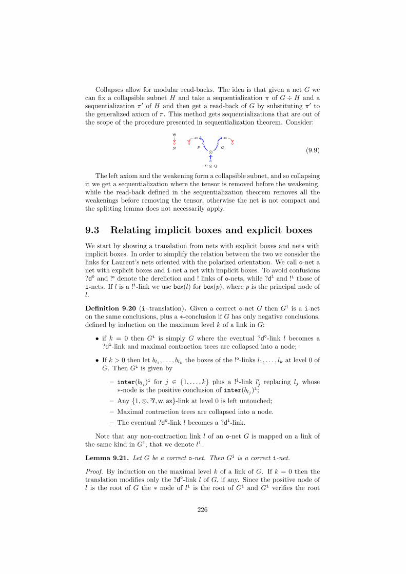
Collapses allow for modular read-backs. The idea is that given a net G wecan fix a collapsible subnet H and take a sequentialization π of G ÷ H and asequentialization π′ of H and then get a read-back of G by substituting π′ tothe generalized axiom of π. This method gets sequentializations that are out ofthe scope of the procedure presented in sequentialization theorem. Consider:

P

ax

Q

ax

P ⊗ Q

⊗N

w

(9.9)

The left axiom and the weakening form a collapsible subnet, and so collapsingit we get a sequentialization where the tensor is removed before the weakening,while the read-back defined in the sequentialization theorem removes all theweakenings before removing the tensor, otherwise the net is not compact andthe splitting lemma does not necessarily apply.

9.3 Relating implicit boxes and explicit boxes

We start by showing a translation from nets with explicit boxes and nets withimplicit boxes. In order to simplify the relation between the two we consider thelinks for Laurent’s nets oriented with the polarized orientation. We call o-net anet with explicit boxes and i-net a net with implicit boxes. To avoid confusions?do and !o denote the dereliction and ! links of o-nets, while ?di and !i those ofi-nets. If l is a !i-link we use box(l) for box(p), where p is the principal node ofl.

Definition 9.20 (i·-translation). Given a correct o-net G then Gi is a i-neton the same conclusions, plus a ∗-conclusion if G has only negative conclusions,defined by induction on the maximum level k of a link in G:

• if k = 0 then Gi is simply G where the eventual ?do-link l becomes a?di-link and maximal contraction trees are collapsed into a node;

• If k > 0 then let bl1 , . . . , blk the boxes of the !o-links l1, . . . , lk at level 0 ofG. Then Gi is given by

– inter(blj )i for j ∈ 1, . . . , k plus a !i-link l′j replacing lj whose

∗-node is the positive conclusion of inter(blj )i;

– Any 1,⊗,`,w, ax-link at level 0 is left untouched;

– Maximal contraction trees are collapsed into a node.

– The eventual ?do-link l becomes a ?di-link.

Note that any non-contraction link l of an o-net G is mapped on a link ofthe same kind in Gi, that we denote li.

Lemma 9.21. Let G be a correct o-net. Then Gi is a correct i-net.

Proof. By induction on the maximal level k of a link of G. If k = 0 then thetranslation modifies only the ?do-link l of G, if any. Since the positive node ofl is the root of G the ∗ node of li is the root of Gi and Gi verifies the root

226

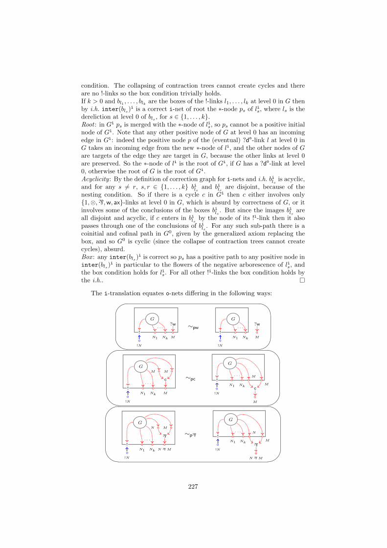
condition. The collapsing of contraction trees cannot create cycles and thereare no !-links so the box condition trivially holds.If k > 0 and bl1 , . . . , blk are the boxes of the !-links l1, . . . , lk at level 0 in G thenby i.h. inter(bls)

i is a correct i-net of root the ∗-node ps of lis, where ls is thedereliction at level 0 of bls , for s ∈ 1, . . . , k.Root : in Gi ps is merged with the ∗-node of lis, so ps cannot be a positive initialnode of Gi. Note that any other positive node of G at level 0 has an incomingedge in Gi: indeed the positive node p of the (eventual) ?do-link l at level 0 inG takes an incoming edge from the new ∗-node of li, and the other nodes of Gare targets of the edge they are target in G, because the other links at level 0are preserved. So the ∗-node of li is the root of Gi, if G has a ?do-link at level0, otherwise the root of G is the root of Gi.Acyclicity : By the definition of correction graph for i-nets and i.h. bils is acyclic,and for any s 6= r, s, r ∈ 1, . . . , k bils and bilr are disjoint, because of thenesting condition. So if there is a cycle c in Gi then c either involves only1,⊗,`,w, ax-links at level 0 in G, which is absurd by correctness of G, or itinvolves some of the conclusions of the boxes bils . But since the images bils areall disjoint and acyclic, if c enters in bils by the node of its !i-link then it alsopasses through one of the conclusions of bils . For any such sub-path there is acoinitial and cofinal path in G0, given by the generalized axiom replacing thebox, and so G0 is cyclic (since the collapse of contraction trees cannot createcycles), absurd.Box : any inter(bls)

i is correct so ps has a positive path to any positive node ininter(bls)

i in particular to the flowers of the negative arborescence of lis, andthe box condition holds for lis. For all other !i-links the box condition holds bythe i.h..

The i-translation equates o-nets differing in the following ways:#

"

!!N

!NkN1

. . .

G

M

?w ∼pw

!N

!NkN1

. . .

G

M

?w

'

&

$

%!N

!NkN1

. . .

G

M

MM

c ∼pc

!N

!NkN1

. . .

G

M

M

M

c

'

&

$

%!N

!NkN1

. . .

G

N `M

MN

` ∼p`

!N

!NkN1

. . .

G

N

M

N `M

`

227

'

&

$

%

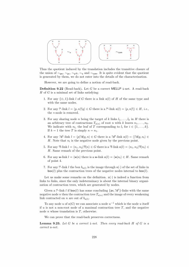
N N

cN

N

c

∼a

N N

cN

N

c

N N

N

c ∼com

N N

N

c

Thus the quotient induced by the translation includes the transitive closure ofthe union of ∼pw, ∼pc, ∼p`, ∼a and ∼com. It is quite evident that the quotientis generated by them, we do not enter into the details of the characterization.

However, we are going to define a notion of read-back.

Definition 9.22 (Read-back). Let G be a correct MELLP i-net. A read-backH of G is a minimal set of links satisfying:

1. For any ⊗, 1-link l of G there is a link o(l) of H of the same type andwith the same nodes.

2. For any !i-link l = 〈p, n|!|q〉 ∈ G there is a !o-link o(l) = 〈p, n|!|〉 ∈ H, i.e.,the ∗-node is removed.

3. For any sharing node n being the target of k links l1, . . . , lk in H there isan arbitrary tree of contractions To(n) of root n with k leaves n1, . . . , nk.We indicate with nli the leaf of T corresponding to li for i ∈ 1, . . . , k.If k = 1 the tree T is simply n = n1.

4. For any ?di-link l = 〈p|?d|q, n〉 ∈ G there is a ?do-link o(l) = 〈|?d|q, nl〉 ∈H. Note that nl is the negative node given by the previous point.

5. For any`-link l = 〈n1, n2|`|n〉 ∈ G there is a`-link o(l) = 〈n1, n2|`|nl〉 ∈H. Same remark of the previous point.

6. For any w-link l = 〈w|n〉 there is a w-link o(l) = 〈w|nl〉 ∈ H. Same remarkof point 4.

7. For any !i-link l the box bo(l) is the image through o(·) of the set of links inbox(l) plus the contraction trees of the negative nodes internal to box(l).

Let us make some remarks on the definition. o(·) is indeed a function fromlinks to links, since the only indeterminacy is about the internal binary organi-zation of contraction trees, which are generated by nodes.

Given a !i-link l if box(l) has some concluding ax, ?di-links with the samenegative node n then the contraction tree To(n) and the image of every weakeninglink contracted on n are out of bo(l).

To any node u of o(G) we can associate a node u−1 which is the node u itselfif u is not a non-root node of a maximal contraction tree T , and the negativenode n whose translation is T , otherwise.

We can prove that the read-back preserves correctness.

Lemma 9.23. Let G be a correct i-net. Then every read-back H of G is acorrect o-net.

228

Proof. H is a o-net by the fact that G is a i-net and the nesting lemma fori-nets.We prove that if G is correct then H0, the correction graph at level 0 of H,is correct. This implies correctness, because implicit boxes are correct, theirinteriors, too, and so by the definition of the translation the other correctiongraphs of H are the correction graph at level 0 of some correct i-net.Any implicit box, being connected, is collapsible and so its replacement witha generalized axiom preserves correctness (corollary 9.19). If we replace anyimplicit box at level 0 we get a net G0 which is correct and with no !-link. Theonly differences between G0 and H0 then are 1) that in G0 the contraction treesof H0 are collapsed into a node and 2) that if there is a dereliction then it hasa conclusion more in G0. It is immediate that these differences cannot alternor acyclicity nor the existence of exactly one positive initial node, so H0 iscorrect.

It is more or less evident that the translation of the read-back is the net westarted with, we do not enter into the details of a formal proof.

229

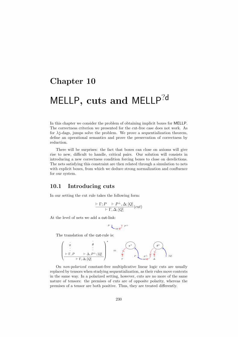
Chapter 10

MELLP, cuts and MELLP?d

In this chapter we consider the problem of obtaining implicit boxes for MELLP.The correctness criterion we presented for the cut-free case does not work. Asfor λj-dags, jumps solve the problem. We prove a sequentialization theorem,define an operational semantics and prove the preservation of correctness byreduction.

There will be surprises: the fact that boxes can close on axioms will giverise to new, difficult to handle, critical pairs. Our solution will consists inintroducing a new correctness condition forcing boxes to close on derelictions.The nets satisfying this constraint are then related through a simulation to netswith explicit boxes, from which we deduce strong normalization and confluencefor our system.

10.1 Introducing cuts

In our setting the cut rule takes the following form:

` Γ;P ` P⊥,∆; [Q]

` Γ,∆; [Q](cut)

At the level of nets we add a cut-link:

P P⊥

cut

The translation of the cut-rule is:.π..

` Γ, P

.

θ..

` ∆, P⊥; [Q]

` Γ,∆; [Q]

?

=

π?

Γ

P

θ?

P⊥∆

[Q]

cut

On non-polarized constant-free multiplicative linear logic cuts are usuallyreplaced by tensors when studying sequentialization, as their rules move contextsin the same way. In a polarized setting, however, cuts are no more of the samenature of tensors: the premises of cuts are of opposite polarity, whereas thepremises of a tensor are both positive. Thus, they are treated differently.

230

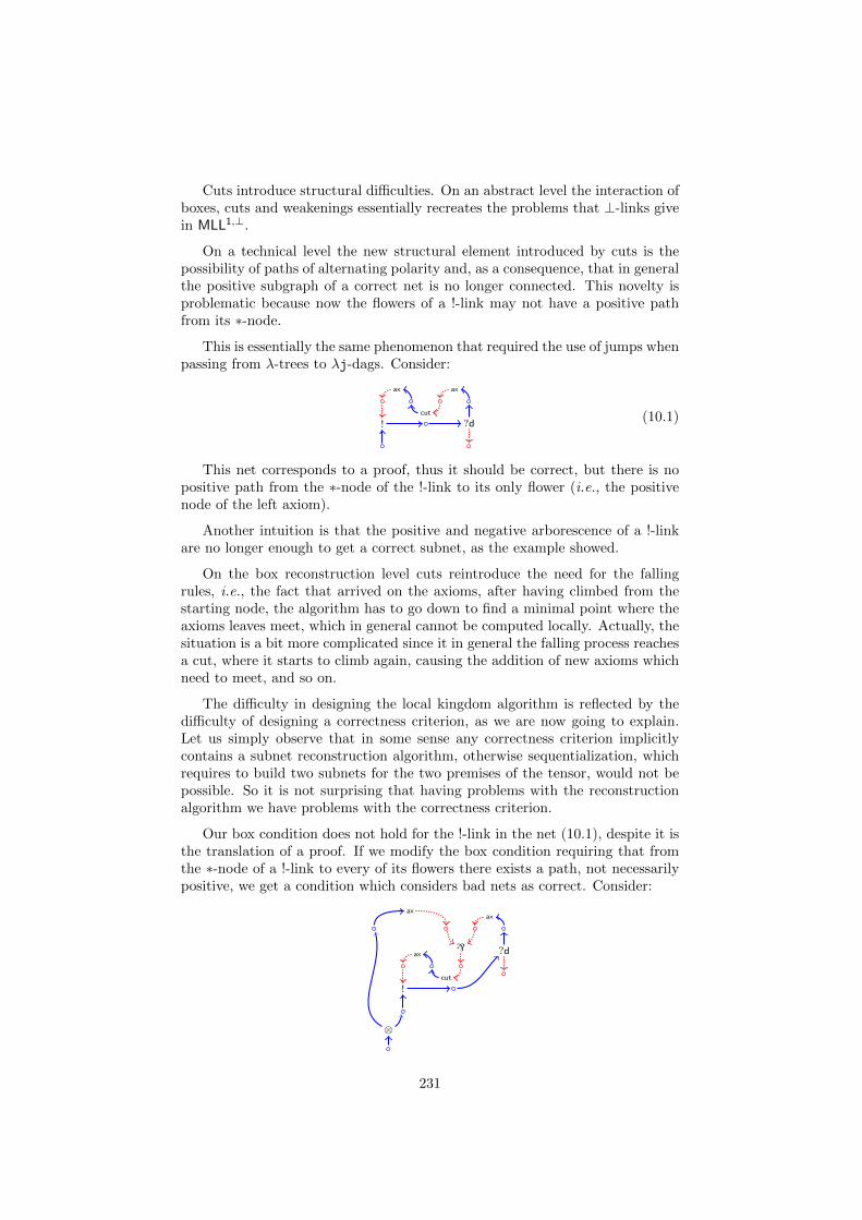
Cuts introduce structural difficulties. On an abstract level the interaction ofboxes, cuts and weakenings essentially recreates the problems that ⊥-links givein MLL1,⊥.

On a technical level the new structural element introduced by cuts is thepossibility of paths of alternating polarity and, as a consequence, that in generalthe positive subgraph of a correct net is no longer connected. This novelty isproblematic because now the flowers of a !-link may not have a positive pathfrom its ∗-node.

This is essentially the same phenomenon that required the use of jumps whenpassing from λ-trees to λj-dags. Consider:

ax

cut

ax

! ?d(10.1)

This net corresponds to a proof, thus it should be correct, but there is nopositive path from the ∗-node of the !-link to its only flower (i.e., the positivenode of the left axiom).

Another intuition is that the positive and negative arborescence of a !-linkare no longer enough to get a correct subnet, as the example showed.

On the box reconstruction level cuts reintroduce the need for the fallingrules, i.e., the fact that arrived on the axioms, after having climbed from thestarting node, the algorithm has to go down to find a minimal point where theaxioms leaves meet, which in general cannot be computed locally. Actually, thesituation is a bit more complicated since it in general the falling process reachesa cut, where it starts to climb again, causing the addition of new axioms whichneed to meet, and so on.

The difficulty in designing the local kingdom algorithm is reflected by thedifficulty of designing a correctness criterion, as we are now going to explain.Let us simply observe that in some sense any correctness criterion implicitlycontains a subnet reconstruction algorithm, otherwise sequentialization, whichrequires to build two subnets for the two premises of the tensor, would not bepossible. So it is not surprising that having problems with the reconstructionalgorithm we have problems with the correctness criterion.

Our box condition does not hold for the !-link in the net (10.1), despite it isthe translation of a proof. If we modify the box condition requiring that fromthe ∗-node of a !-link to every of its flowers there exists a path, not necessarilypositive, we get a condition which considers bad nets as correct. Consider:

ax

cut

`

axax

!

?d

⊗

231

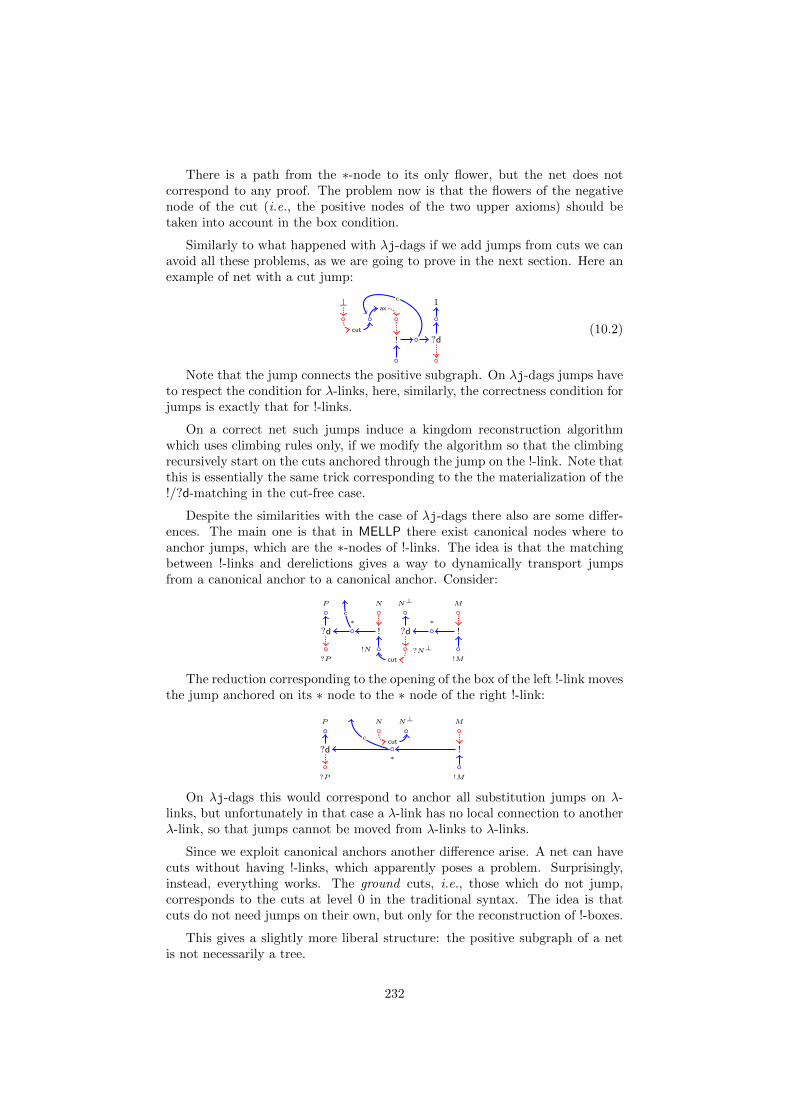
There is a path from the ∗-node to its only flower, but the net does notcorrespond to any proof. The problem now is that the flowers of the negativenode of the cut (i.e., the positive nodes of the two upper axioms) should betaken into account in the box condition.

Similarly to what happened with λj-dags if we add jumps from cuts we canavoid all these problems, as we are going to prove in the next section. Here anexample of net with a cut jump:

ax⊥

cut

1

! ?d

c

(10.2)

Note that the jump connects the positive subgraph. On λj-dags jumps haveto respect the condition for λ-links, here, similarly, the correctness condition forjumps is exactly that for !-links.

On a correct net such jumps induce a kingdom reconstruction algorithmwhich uses climbing rules only, if we modify the algorithm so that the climbingrecursively start on the cuts anchored through the jump on the !-link. Note thatthis is essentially the same trick corresponding to the the materialization of the!/?d-matching in the cut-free case.

Despite the similarities with the case of λj-dags there also are some differ-ences. The main one is that in MELLP there exist canonical nodes where toanchor jumps, which are the ∗-nodes of !-links. The idea is that the matchingbetween !-links and derelictions gives a way to dynamically transport jumpsfrom a canonical anchor to a canonical anchor. Consider:

?P

P

?d

!N

N

!∗

?N⊥

N⊥

?d

!M

M

!∗

cut

c

The reduction corresponding to the opening of the box of the left !-link movesthe jump anchored on its ∗ node to the ∗ node of the right !-link:

?P

P

?d

N N⊥

!M

M

!∗

cutc

On λj-dags this would correspond to anchor all substitution jumps on λ-links, but unfortunately in that case a λ-link has no local connection to anotherλ-link, so that jumps cannot be moved from λ-links to λ-links.

Since we exploit canonical anchors another difference arise. A net can havecuts without having !-links, which apparently poses a problem. Surprisingly,instead, everything works. The ground cuts, i.e., those which do not jump,corresponds to the cuts at level 0 in the traditional syntax. The idea is thatcuts do not need jumps on their own, but only for the reconstruction of !-boxes.

This gives a slightly more liberal structure: the positive subgraph of a netis not necessarily a tree.

232

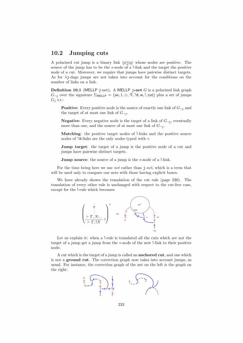
10.2 Jumping cuts

A polarized cut jump is a binary link 〈p|j|q〉 whose nodes are positive. Thesource of the jump has to be the ∗-node of a !-link and the target the positivenode of a cut. Moreover, we require that jumps have pairwise distinct targets.As for λj-dags jumps are not taken into account for the conditions on thenumber of links on a link.

Definition 10.1 (MELLP j-net). A MELLP j-net G is a polarized link graphG¬j over the signature ΣMELLP = ax, 1,⊗,`, ?d,w, !, cut plus a set of jumpsGj s.t.:

Positive: Every positive node is the source of exactly one link of G¬j andthe target of at most one link of G¬j.

Negative: Every negative node is the target of a link of G¬j, eventuallymore than one, and the source of at most one link of G¬j.

Matching: the positive target nodes of !-links and the positive sourcenodes of ?d-links are the only nodes typed with ∗.

Jump target: the target of a jump is the positive node of a cut andjumps have pairwise distinct targets.

Jump source: the source of a jump is the ∗-node of a !-link.

For the time being here we use net rather than j-net, which is a term thatwill be used only to compare our nets with those having explicit boxes.

We have already shown the translation of the cut rule (page 230). Thetranslation of every other rule is unchanged with respect to the cut-free case,except for the !-rule which becomes:

.π..

` Γ, N ;!` Γ; !N

?

=

π?

∗ N

Γ

cuts

!N

!

c

Let us explain it: when a !-rule is translated all the cuts which are not thetarget of a jump get a jump from the ∗-node of the new !-link to their positivenode.

A cut which is the target of a jump is called an anchored cut, and one whichis not a ground cut. The correction graph now takes into account jumps, asusual. For instance, the correction graph of the net on the left is the graph onthe right:

ax⊥

cut

1

! ?d

c

233

The dashed edges are those whose node have different polarity. Note thatjumps induces positive edges. The root and the DAG condition are defined asbefore. We get:

Lemma 10.2 (forest structure). Let G be a net satisfying the root and DAGconditions. In G∗:

1. Positive nodes and positive paths form a directed forest.

2. Negative nodes and negative paths form a directed forest.

Proof. 1) By the DAG condition G∗ is acyclic. By the shape of links anddefinition of the correction graph positive nodes have at most one incomingpositive edge.2) By the shape of links no negative node has two outgoing negative edges.

A simple inspection of the shape of the links and the conditions on netsshows that the roots of the maximal negative trees, i.e., the negative ends,now can be the negative conclusions of a net, the negative node of a !-link andthe negative node of a cut. The third case is the new one. The roots of thepositive trees, called positive starts, are the positive nodes of ground cuts andthe root of the net.

The arborescence of a negative node is defined as before. That one of apositive node now also includes the jumps. More precisely, we establish thatthe principal node of a jump is its source node and then use essentially the samedefinition as before, namely:

Definition 10.3 (arborescence). Let G be a net. The arborescence arb(p) ofa positive node p is the set of positive links and jumps s.t. p has a positive pathto their positive principal node.

Flowers are defined as in the cut-free case. Jumps for cuts and !-links aresubject to the same correctness condition, so we treat them compactly. !-linksand anchored cuts are boxing links. Every boxing link has an associatedboxing node: for a !-link is its ∗-node and for an anchored cut link l is the∗-node of the !-link jumping on l. Note that the boxing node of an anchored cutl is not a node of l, but it is next to it. A node/link in the negative arborescenceof a boxing link l is boxed by l, or boxed by p if p is the boxing node of l, orsimply boxed.

Definition 10.4 (correct net). Let G be a net. G is correct when G∗ satisfiesthe following conditions:

• Root: there is only one positive entry node.

• DAG: it is acyclic.

• Box: for every boxing link l the flowers of its negative arborescence havea positive path from the boxing node of l.

234

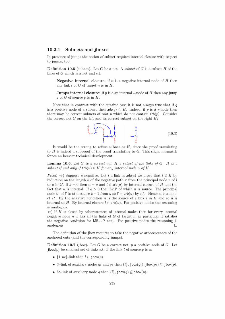
10.2.1 Subnets and jboxes

In presence of jumps the notion of subnet requires internal closure with respectto jumps, too:

Definition 10.5 (subnet). Let G be a net. A subnet of G is a subset H of thelinks of G which is a net and s.t.

Negative internal closure: if n is a negative internal node of H thenany link l of G of target n is in H.

Jumps internal closure: if p is a an internal ∗-node of H then any jumpj of G of source p is in H.

Note that in contrast with the cut-free case it is not always true that if qis a positive node of a subnet then arb(q) ⊆ H. Indeed, if p is a ∗-node thenthere may be correct subnets of root p which do not contain arb(p). Considerthe correct net G on the left and its correct subnet on the right H:

ax⊥

cut

1

! ?d

c 1

?d(10.3)

It would be too strong to refuse subnet as H, since the proof translatingto H is indeed a subproof of the proof translating to G. This slight mismatchforces an heavier technical development.

Lemma 10.6. Let G be a correct net, H a subset of the links of G. H is asubnet if and only if arb(u) ∈ H for any internal node u of H.

Proof. ⇒) Suppose u negative. Let l a link in arb(u) we prove that l ∈ H byinduction on the length k of the negative path τ from the principal node n of lto u in G. If k = 0 then n = u and l ∈ arb(u) by internal closure of H and thefact that u is internal. If k > 0 the link l′ of which n is source. The principalnode n′ of l′ is at distance k− 1 from u so l′ ∈ arb(u) by i.h.. Hence n is a nodeof H. By the negative condition n is the source of a link i in H and so n isinternal to H. By internal closure l ∈ arb(u). For positive nodes the reasoningis analogous.⇐) If H is closed by arborescences of internal nodes then for every internalnegative node n it has all the links of G of target n, in particular it satisfiesthe negative condition for MELLP nets. For positive nodes the reasoning isanalogous.

The definition of the jbox requires to take the negative arborescences of theanchored cuts (and the corresponding jumps).

Definition 10.7 (jbox). Let G be a correct net, p a positive node of G. Letjbox(p) be smallest set of links s.t. if the link l of source p is a:

• 1, ax-link then l ∈ jbox(p).

• ⊗-link of auxiliary nodes q1 and q2 then l, jbox(q1), jbox(q2) ⊆ jbox(p).

• ?d-link of auxiliary node q then l, jbox(q) ⊆ jbox(p).

235

• !-link l = 〈n, p|!|q〉 with h jumps ji from q to h cuts li = 〈mi|cut|qi〉, withi ∈ 1, . . . , h, then l, jbox(q), arbG(n) ⊆ jbox(p) and li, ji, arbG(mi) ⊆jbox(p).

Jboxes are subject to the same slight technical inconvenient of general sub-nets, that is, it is no longer true that arb(q) ⊆ jbox(p) for any positive nodeq in jbox(p). It certainly holds for the internal nodes, as we will prove thatjbox(p) is a subnet, but if p is a ∗-node which is the anchor of some jump thenarb(p) ⊆ jbox(p) does not hold (example (10.3)). However, when p is not a∗-node we get arb(p) ⊆ jbox(p). The next lemma formalize this:

Lemma 10.8 (positive paths and jboxes). Let G be a correct net, p a positivenode of G.

1. Every positive node q in jbox(p) has a positive path from p and jbox(q) ⊆jbox(p).

2. If p is not a ∗-node or it is a positive start of G then arb(p) ⊆ jbox(p).

Proof. We prove both points together by induction on the definition of jbox(p).If p is the principal node of a:

• 1, ax-link l: then the only positive node of jbox(p) is p.

• ?d-link l of positive target q: all the positive nodes of jbox(p) are thoseof jbox(q) plus p. By i.h. any positive node q′ in jbox(q) has a positivepath from q and jbox(q′) ⊆ jbox(q). We get point 1 since p has a positiveedge to q and jbox(q) ⊆ jbox(p) by definition. Point 2: by i.h. arb(q) ⊆jbox(q) since q cannot be a ∗ node. If p is the root then there are nojumps anchored on it, because it cannot be the node of a !-link, andits arborescence is given by arb(q) and l, so arb(p) ⊆ jbox(p). By thematching condition p cannot be a positive start of G.

• ⊗-link l of targets q1 and q2: the first point uses the i.h., as in the previouscase. Point 2: by the matching condition q1 and q2 cannot be ∗-nodes, soby i.h. arb(qi) ⊆ jbox(qi) for i = 1, 2, and thus arb(p) ⊆ jbox(p).

• !-link l = 〈n, p|!|q〉. Let q1, . . . , qk the positive nodes of cut links l1, . . . , lktarget of jumps j1, . . . , jk from q and let S = q, q1, . . . , qk. By i.h.jbox(x) satisfies point 1 for x ∈ S, and p, having a positive path to everyx ∈ S, has a positive path to every positive node q′ in

⋃x∈S jbox(x).

Moreover jbox(q′) ⊆ jbox(p), and⋃x∈S jbox(x) ⊆ jbox(p) by definition.

The only positive nodes of jbox(p) which may not be in⋃x∈S jbox(x) are

the flowers of the negative nodes of l, l1, . . . , lk. By correctness of G we getthat these flowers have a positive path from q, which is the boxing nodeof l, l1, . . . , lk, and thus a positive path from p and their jbox is containedin jbox(p).Point 2: for all nodes x in S \ q we get arb(x) ⊆ jbox(x). Thus jbox(p)takes all the jumps from q and all the positive arborescences of theirtargets, so that arb(q) ⊆ jbox(p), and so arb(p) ⊆ jbox(p).

From the previous lemma we easily get:

236

Proposition 10.9 (kingdom). Let G be a correct net, p a positive node of G.jbox(p) is a correct subnet of G of root p. Moreover, it is the smallest such one,it has no w,`-conclusion and no ground cut.

Modulo the presence of jumps this proof is essentially as in the cut-free case.

Proof. By induction on the definition of jbox(p). The only interesting case isthe one for p conclusion of a !-link l = 〈n, p|!|q〉. By lemma 10.8 we get thatjbox(p) satisfies the root condition. Let q1, . . . , qk the positive nodes of cut linksl1, . . . , lk target of jumps j1, . . . , jk from q and let S = q, q1, . . . , qk. By i.h.jbox(x) is a subnet for x ∈ S so it is internally closed. And arborescences areinternally closed sets of links. By the definition of jbox jbox(p) contains all thejumps from the ∗-node q of l so it is internally closed. Moreover, by lemma 10.8any positive node respects the positive condition. The negative nodes respectthe negative condition because they belong either to jbox(x) for some x ∈ S orto some arborescence. So jbox(p) is a subnet of G. The boxing links l, l1, . . . , lksatisfy the box condition, since they all have q as boxing node and by lemma10.8 all the flowers of their negative arborescences have a path from p, and thusfrom q. Any other boxing link is in jbox(x) for some x ∈ S, and so the boxcondition holds for it by the i.h.. Hence jbox(p) satisfies the box condition, andit is correct.By i.h. jbox(x) is the kingdom of x ∈ S so jbox(p) is the kingdom of p, becauseany other correct subnet not containing jbox(y) for some y ∈ S would notbe internally closed with respect to q, which is an internal node of any subnetcontaining l. By i.h. no w,`-conclusion nor ground cut belongs to any jbox(x)and they are not added in the !-case.

And:

Proposition 10.10 (nesting property). Let G be a correct net. If jbox(p) ∩jbox(q) 6= ∅ then either jbox(p) ⊆ jbox(q) or jbox(q) ⊆ jbox(p).

This proof is essentially as that one in the cut-free case, too.

Proof. Suppose that I := jbox(p)∩jbox(q) contains a link with a positive nodep′. Lemma 10.8 implies that p′ has a positive path νp from p and a positivepath νq from q. Since the positive graph is a forest νp and νq are both suffixesof the unique positive path ν from a positive start of G to p′. So either q is onνp or p on νq. Suppose wlog to be in the first case. Then q ∈ jbox(p) and bylemma 10.8 we get jbox(q) ⊆ jbox(p).Now suppose that I contains a link l with no positive node, i.e., a w,`-link.Boxes have no concluding link which is a w,`-link so in both boxes l belongsto the negative arborescence a boxing link i. This implies i ∈ I. But i has apositive node, so we conclude.

10.2.2 Sequentialization

Sequentialization in presence of cuts is slightly more elaborated than in the cut-free case, and it is essentially as for λj-dags. We have to understand when it issafe to remove cuts, i.e., when the removal of a cut splits the net in two disjointcorrect nets. The role played by the jumps anchored on the root in the case ofλj-dags is here played by the ground cuts, i.e., those without a jump on them.

237

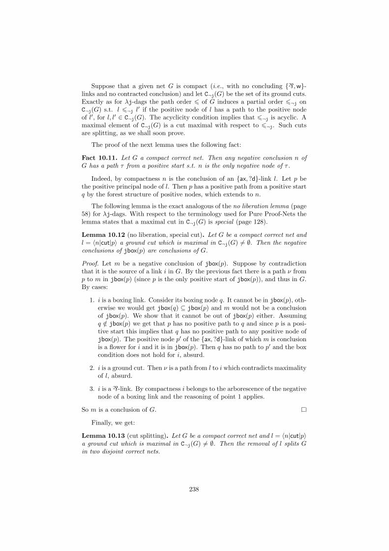
Suppose that a given net G is compact (i.e., with no concluding `,w-links and no contracted conclusion) and let C¬j(G) be the set of its ground cuts.Exactly as for λj-dags the path order 6 of G induces a partial order 6¬j onC¬j(G) s.t. l 6¬j l′ if the positive node of l has a path to the positive nodeof l′, for l, l′ ∈ C¬j(G). The acyclicity condition implies that 6¬j is acyclic. Amaximal element of C¬j(G) is a cut maximal with respect to 6¬j. Such cutsare splitting, as we shall soon prove.

The proof of the next lemma uses the following fact:

Fact 10.11. Let G a compact correct net. Then any negative conclusion n ofG has a path τ from a positive start s.t. n is the only negative node of τ .

Indeed, by compactness n is the conclusion of an ax, ?d-link l. Let p bethe positive principal node of l. Then p has a positive path from a positive startq by the forest structure of positive nodes, which extends to n.

The following lemma is the exact analogous of the no liberation lemma (page58) for λj-dags. With respect to the terminology used for Pure Proof-Nets thelemma states that a maximal cut in C¬j(G) is special (page 128).

Lemma 10.12 (no liberation, special cut). Let G be a compact correct net andl = 〈n|cut|p〉 a ground cut which is maximal in C¬j(G) 6= ∅. Then the negativeconclusions of jbox(p) are conclusions of G.

Proof. Let m be a negative conclusion of jbox(p). Suppose by contradictionthat it is the source of a link i in G. By the previous fact there is a path ν fromp to m in jbox(p) (since p is the only positive start of jbox(p)), and thus in G.By cases:

1. i is a boxing link. Consider its boxing node q. It cannot be in jbox(p), oth-erwise we would get jbox(q) ⊆ jbox(p) and m would not be a conclusionof jbox(p). We show that it cannot be out of jbox(p) either. Assumingq /∈ jbox(p) we get that p has no positive path to q and since p is a posi-tive start this implies that q has no positive path to any positive node ofjbox(p). The positive node p′ of the ax, ?d-link of which m is conclusionis a flower for i and it is in jbox(p). Then q has no path to p′ and the boxcondition does not hold for i, absurd.

2. i is a ground cut. Then ν is a path from l to i which contradicts maximalityof l, absurd.

3. i is a `-link. By compactness i belongs to the arborescence of the negativenode of a boxing link and the reasoning of point 1 applies.

So m is a conclusion of G.

Finally, we get:

Lemma 10.13 (cut splitting). Let G be a compact correct net and l = 〈n|cut|p〉a ground cut which is maximal in C¬j(G) 6= ∅. Then the removal of l splits Gin two disjoint correct nets.

238

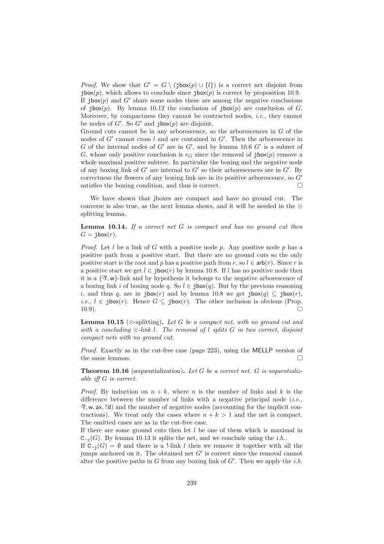
Proof. We show that G′ = G \ (jbox(p) ∪ l) is a correct net disjoint fromjbox(p), which allows to conclude since jbox(p) is correct by proposition 10.9.If jbox(p) and G′ share some nodes these are among the negative conclusionsof jbox(p). By lemma 10.12 the conclusion of jbox(p) are conclusion of G.Moreover, by compactness they cannot be contracted nodes, i.e., they cannotbe nodes of G′. So G′ and jbox(p) are disjoint.Ground cuts cannot be in any arborescence, so the arborescences in G of thenodes of G′ cannot cross l and are contained in G′. Then the arborescence inG of the internal nodes of G′ are in G′, and by lemma 10.6 G′ is a subnet ofG, whose only positive conclusion is rG since the removal of jbox(p) remove awhole maximal positive subtree. In particular the boxing and the negative nodeof any boxing link of G′ are internal to G′ so their arborescences are in G′. Bycorrectness the flowers of any boxing link are in its positive arborescence, so G′

satisfies the boxing condition, and thus is correct.

We have shown that jboxes are compact and have no ground cut. Theconverse is also true, as the next lemma shows, and it will be needed in the ⊗splitting lemma.

Lemma 10.14. If a correct net G is compact and has no ground cut thenG = jbox(r).

Proof. Let l be a link of G with a positive node p. Any positive node p has apositive path from a positive start. But there are no ground cuts so the onlypositive start is the root and p has a positive path from r, so l ∈ arb(r). Since r isa positive start we get l ∈ jbox(r) by lemma 10.8. If l has no positive node thenit is a `,w-link and by hypothesis it belongs to the negative arborescence ofa boxing link i of boxing node q. So l ∈ jbox(q). But by the previous reasoningi, and thus q, are in jbox(r) and by lemma 10.8 we get jbox(q) ⊆ jbox(r),i.e., l ∈ jbox(r). Hence G ⊆ jbox(r). The other inclusion is obvious (Prop.10.9).

Lemma 10.15 (⊗-splitting). Let G be a compact net, with no ground cut andwith a concluding ⊗-link l. The removal of l splits G in two correct, disjointcompact nets with no ground cut.

Proof. Exactly as in the cut-free case (page 223), using the MELLP version ofthe same lemmas.

Theorem 10.16 (sequentialization). Let G be a correct net. G is sequentializ-able iff G is correct.

Proof. By induction on n + k, where n is the number of links and k is thedifference between the number of links with a negative principal node (i.e.,`,w, ax, ?d) and the number of negative nodes (accounting for the implicit con-tractions). We treat only the cases where n + k > 1 and the net is compact.The omitted cases are as in the cut-free case.If there are some ground cuts then let l be one of them which is maximal inC¬j(G). By lemma 10.13 it splits the net, and we conclude using the i.h..If C¬j(G) = ∅ and there is a !-link l then we remove it together with all thejumps anchored on it. The obtained net G′ is correct since the removal cannotalter the positive paths in G from any boxing link of G′. Then we apply the i.h.

239

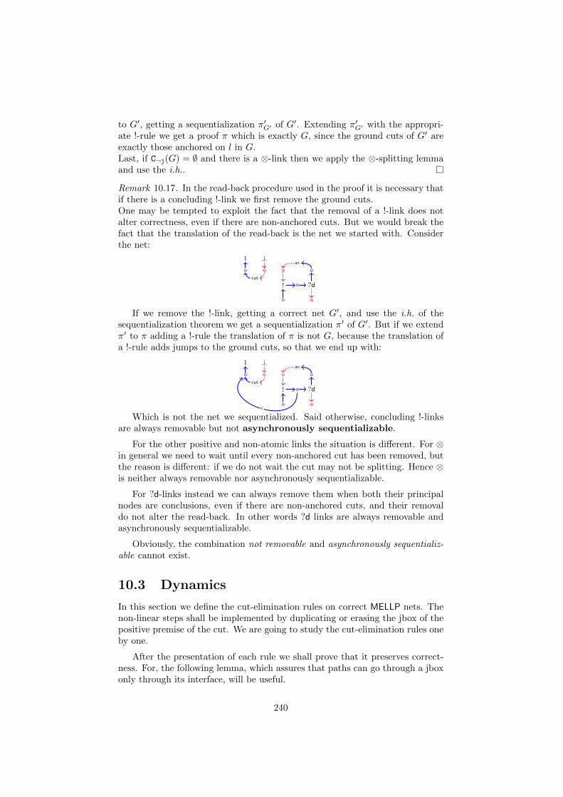
to G′, getting a sequentialization π′G′ of G′. Extending π′G′ with the appropri-ate !-rule we get a proof π which is exactly G, since the ground cuts of G′ areexactly those anchored on l in G.Last, if C¬j(G) = ∅ and there is a ⊗-link then we apply the ⊗-splitting lemmaand use the i.h..

Remark 10.17. In the read-back procedure used in the proof it is necessary thatif there is a concluding !-link we first remove the ground cuts.One may be tempted to exploit the fact that the removal of a !-link does notalter correctness, even if there are non-anchored cuts. But we would break thefact that the translation of the read-back is the net we started with. Considerthe net:

ax

! ?d

⊥1

cut

If we remove the !-link, getting a correct net G′, and use the i.h. of thesequentialization theorem we get a sequentialization π′ of G′. But if we extendπ′ to π adding a !-rule the translation of π is not G, because the translation ofa !-rule adds jumps to the ground cuts, so that we end up with:

ax

! ?d

⊥1

cut

c

Which is not the net we sequentialized. Said otherwise, concluding !-linksare always removable but not asynchronously sequentializable.

For the other positive and non-atomic links the situation is different. For ⊗in general we need to wait until every non-anchored cut has been removed, butthe reason is different: if we do not wait the cut may not be splitting. Hence ⊗is neither always removable nor asynchronously sequentializable.

For ?d-links instead we can always remove them when both their principalnodes are conclusions, even if there are non-anchored cuts, and their removaldo not alter the read-back. In other words ?d links are always removable andasynchronously sequentializable.

Obviously, the combination not removable and asynchronously sequentializ-able cannot exist.

10.3 Dynamics

In this section we define the cut-elimination rules on correct MELLP nets. Thenon-linear steps shall be implemented by duplicating or erasing the jbox of thepositive premise of the cut. We are going to study the cut-elimination rules oneby one.

After the presentation of each rule we shall prove that it preserves correct-ness. For, the following lemma, which assures that paths can go through a jboxonly through its interface, will be useful.

240

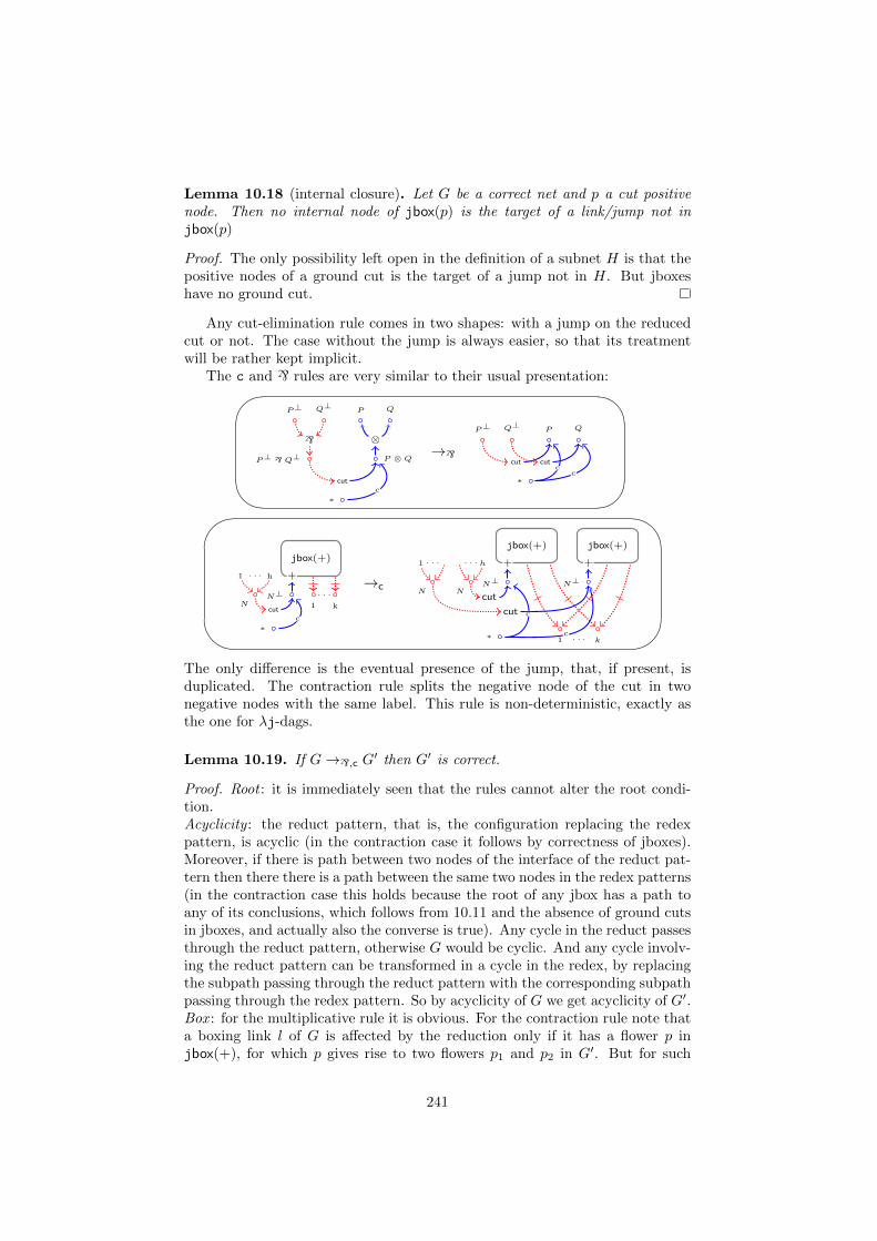
Lemma 10.18 (internal closure). Let G be a correct net and p a cut positivenode. Then no internal node of jbox(p) is the target of a link/jump not injbox(p)

Proof. The only possibility left open in the definition of a subnet H is that thepositive nodes of a ground cut is the target of a jump not in H. But jboxeshave no ground cut.

Any cut-elimination rule comes in two shapes: with a jump on the reducedcut or not. The case without the jump is always easier, so that its treatmentwill be rather kept implicit.

The c and ` rules are very similar to their usual presentation:#

"

!P ⊗ Q

P Q

⊗

P⊥ ` Q⊥

P⊥ Q⊥

`

cut

∗c

→`

P QQ⊥P⊥

cut cut

∗

cc

'

&

$

%N

1 h. . .

N⊥

+

k1

jbox(+)

. . .

cut

∗c

→cN

1 . . .

N

h. . .

N⊥

+

jbox(+)

cut

N⊥

+

jbox(+)

1 k. . .

cut

∗

c

c

The only difference is the eventual presence of the jump, that, if present, isduplicated. The contraction rule splits the negative node of the cut in twonegative nodes with the same label. This rule is non-deterministic, exactly asthe one for λj-dags.

Lemma 10.19. If G→`,c G′ then G′ is correct.

Proof. Root : it is immediately seen that the rules cannot alter the root condi-tion.Acyclicity : the reduct pattern, that is, the configuration replacing the redexpattern, is acyclic (in the contraction case it follows by correctness of jboxes).Moreover, if there is path between two nodes of the interface of the reduct pat-tern then there there is a path between the same two nodes in the redex patterns(in the contraction case this holds because the root of any jbox has a path toany of its conclusions, which follows from 10.11 and the absence of ground cutsin jboxes, and actually also the converse is true). Any cycle in the reduct passesthrough the reduct pattern, otherwise G would be cyclic. And any cycle involv-ing the reduct pattern can be transformed in a cycle in the redex, by replacingthe subpath passing through the reduct pattern with the corresponding subpathpassing through the redex pattern. So by acyclicity of G we get acyclicity of G′.Box : for the multiplicative rule it is obvious. For the contraction rule note thata boxing link l of G is affected by the reduction only if it has a flower p injbox(+), for which p gives rise to two flowers p1 and p2 in G′. But for such

241

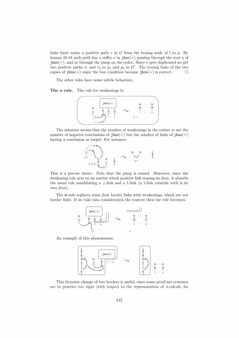
links there exists a positive path τ in G from the boxing node of l to p. Bylemma 10.18 such path has a suffix ν in jbox(+) passing through the root q ofjbox(+), and so through the jump on the redex. Since ν gets duplicated we gettwo positive paths τ1 and τ2 to p1 and p2 in G′. The boxing links of the twocopies of jbox(+) enjoy the box condition because jbox(+) is correct.

The other rules have some subtle behaviors.

The w rule. The rule for weakenings is:#

"

!w +

k1

jbox(+)

cut

∗c

→w1 k

w w. . .

. . .

∗

The notation means that the number of weakenings in the reduct is not thenumber of negative conclusions of jbox(+) but the number of links of jbox(+)having a conclusion as target. For instance:

P ⊗ P

⊗P⊥

ax

ax

w

cut

1→w

P⊥

w w 1

This is a precise choice. Note that the jump is erased. Moreover, since theweakening rule acts on no matter which positive link erasing its jbox, it absorbsthe usual rule annihilating a ⊥-link and a 1-link (a 1-link coincide with is itsown jbox).

The w-rule replaces some jbox border links with weakenings, which are notborder links. If we take into consideration the context then the rule becomes:

w +

k1

jbox(+)

cut

...

c

→w

1 k

w w. . .

. . .

...

An example of this phenomenon:

w

1

?d !k1 . . .

jbox(!)

!cut

c

→w

1

?d

!1 k

w w. . .

. . .

This dynamic change of box borders is useful, since some proof net syntaxesare in practice too rigid (with respect to the representation of λ-calculi, for

242

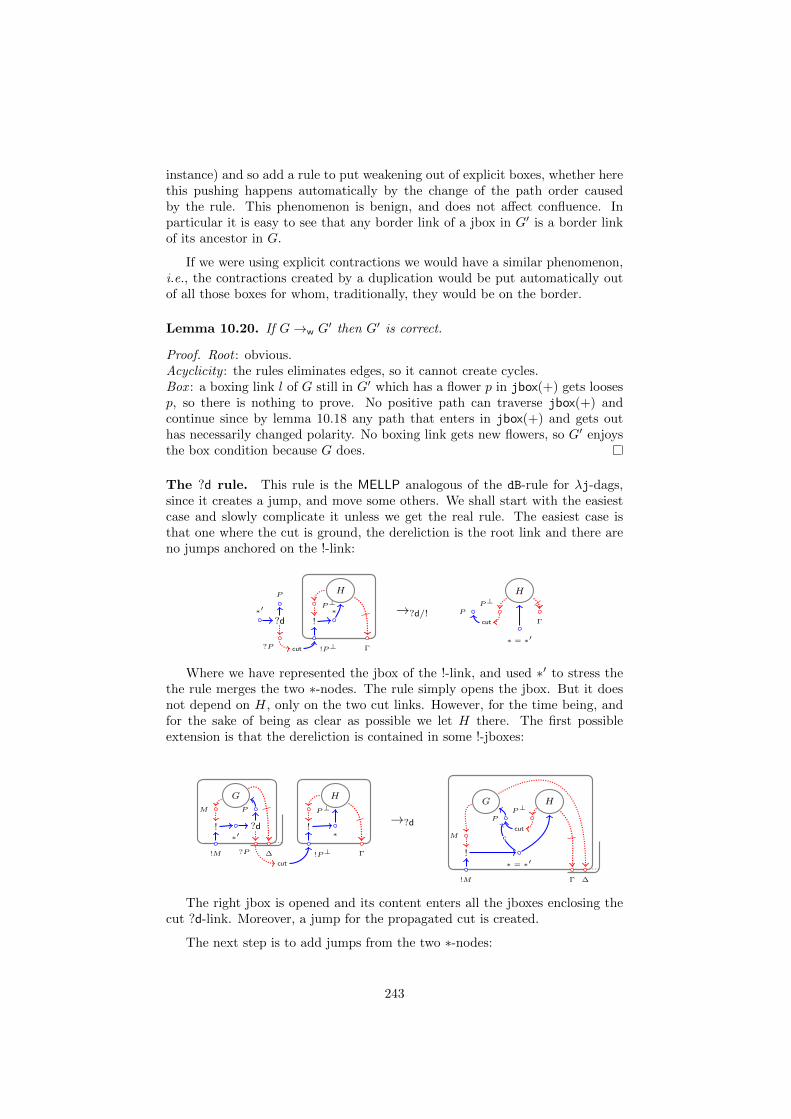
instance) and so add a rule to put weakening out of explicit boxes, whether herethis pushing happens automatically by the change of the path order causedby the rule. This phenomenon is benign, and does not affect confluence. Inparticular it is easy to see that any border link of a jbox in G′ is a border linkof its ancestor in G.

If we were using explicit contractions we would have a similar phenomenon,i.e., the contractions created by a duplication would be put automatically outof all those boxes for whom, traditionally, they would be on the border.

Lemma 10.20. If G→w G′ then G′ is correct.

Proof. Root : obvious.Acyclicity : the rules eliminates edges, so it cannot create cycles.Box : a boxing link l of G still in G′ which has a flower p in jbox(+) gets loosesp, so there is nothing to prove. No positive path can traverse jbox(+) andcontinue since by lemma 10.18 any path that enters in jbox(+) and gets outhas necessarily changed polarity. No boxing link gets new flowers, so G′ enjoysthe box condition because G does.

The ?d rule. This rule is the MELLP analogous of the dB-rule for λj-dags,since it creates a jump, and move some others. We shall start with the easiestcase and slowly complicate it unless we get the real rule. The easiest case isthat one where the cut is ground, the dereliction is the root link and there areno jumps anchored on the !-link:

?P

P

∗′

?d

!P⊥

P⊥∗

!

cut Γ

H

→?d/! PP⊥

cut

∗ = ∗′

H

Γ

Where we have represented the jbox of the !-link, and used ∗′ to stress thethe rule merges the two ∗-nodes. The rule simply opens the jbox. But it doesnot depend on H, only on the two cut links. However, for the time being, andfor the sake of being as clear as possible we let H there. The first possibleextension is that the dereliction is contained in some !-jboxes:

?P

P

∗′?d

!P⊥

P⊥

∗!

cut

M

!M

!

Γ

HG

∆

...

→?dP

P⊥

cutM

!M

!∗ = ∗′

c

G

Γ ∆

...

H

The right jbox is opened and its content enters all the jboxes enclosing thecut ?d-link. Moreover, a jump for the propagated cut is created.

The next step is to add jumps from the two ∗-nodes:

243

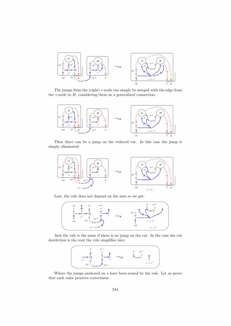
?P

P

∗′?d

!P⊥

P⊥

∗!

cut

M

!M

!

Γ

H

c

G

c

∆

...

→?dP

P⊥

cutM

!M

!∗ = ∗′

c

G

c

Γ ∆

...

H

c

The jumps from the (right) ∗-node can simply be merged with the edge fromthe ∗-node to H, considering them as a generalized connection:

?P

P

∗′?d

!P⊥

P⊥

∗!

cut

M

!M

!

Γ

HG

c

∆

...

→?dP

P⊥

cutM

!M

!∗ = ∗′

c

G

c

Γ ∆

...

H

Then there can be a jump on the reduced cut. In this case the jump issimply eliminated:

?P

P

∗′?d

!P⊥

P⊥

∗!

cut

∗′′c

M

!M

!

Γ

HG

c

∆

...

→?dP

P⊥

cutM

!M

! ∗ = ∗′

∗′′

c

G

c

Γ ∆

...

H

Last, the rule does not depend on the nets so we get:#

"

!?P

P

?d

!P⊥

P⊥

∗!

cut

∗′′c

M

!M

!∗′

c

→?d

P P⊥

cutM

!M

!∗ = ∗′

cc

∗′′

And the rule is the same if there is no jump on the cut. In the case the cutdereliction is the root the rule simplifies into:

?P

P

?d

!P⊥

P⊥

∗!

cut

∗′→?d′

P P⊥

cut

∗ = ∗′

Where the jumps anchored on ∗ have been erased by the rule. Let us provethat such rules preserve correctness.

244

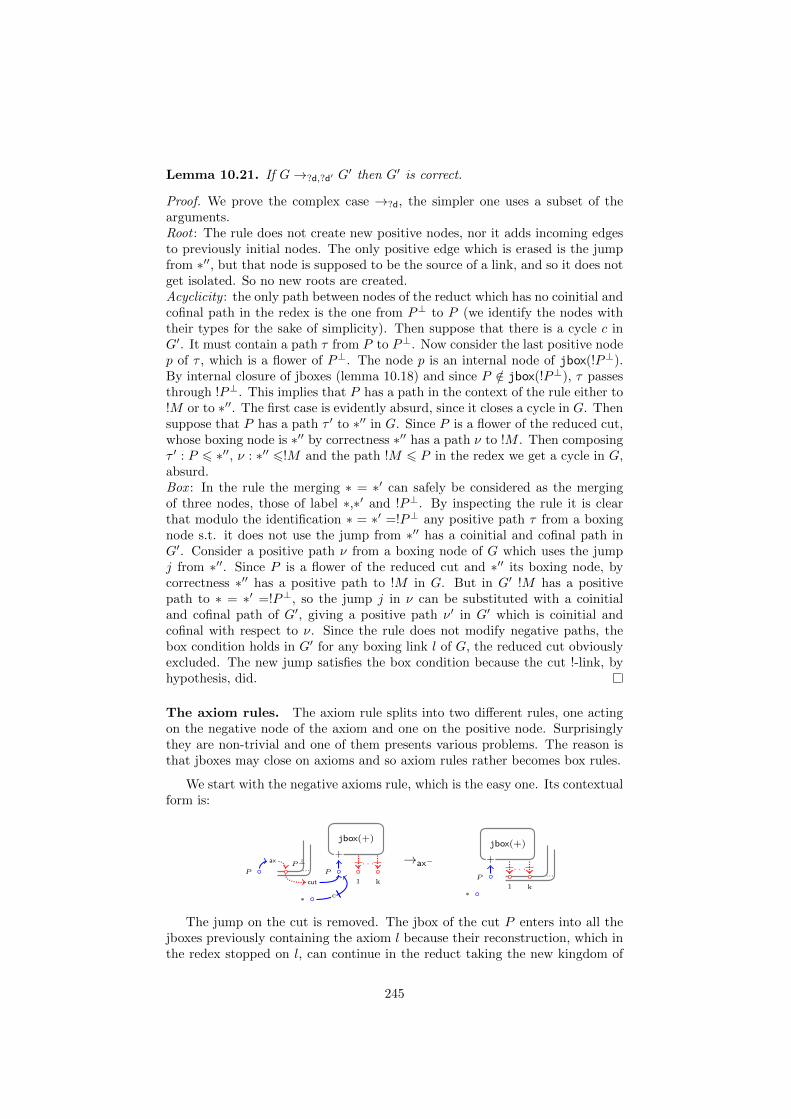
Lemma 10.21. If G→?d,?d′ G′ then G′ is correct.

Proof. We prove the complex case →?d, the simpler one uses a subset of thearguments.Root : The rule does not create new positive nodes, nor it adds incoming edgesto previously initial nodes. The only positive edge which is erased is the jumpfrom ∗′′, but that node is supposed to be the source of a link, and so it does notget isolated. So no new roots are created.Acyclicity : the only path between nodes of the reduct which has no coinitial andcofinal path in the redex is the one from P⊥ to P (we identify the nodes withtheir types for the sake of simplicity). Then suppose that there is a cycle c inG′. It must contain a path τ from P to P⊥. Now consider the last positive nodep of τ , which is a flower of P⊥. The node p is an internal node of jbox(!P⊥).By internal closure of jboxes (lemma 10.18) and since P /∈ jbox(!P⊥), τ passesthrough !P⊥. This implies that P has a path in the context of the rule either to!M or to ∗′′. The first case is evidently absurd, since it closes a cycle in G. Thensuppose that P has a path τ ′ to ∗′′ in G. Since P is a flower of the reduced cut,whose boxing node is ∗′′ by correctness ∗′′ has a path ν to !M . Then composingτ ′ : P 6 ∗′′, ν : ∗′′ 6!M and the path !M 6 P in the redex we get a cycle in G,absurd.Box : In the rule the merging ∗ = ∗′ can safely be considered as the mergingof three nodes, those of label ∗,∗′ and !P⊥. By inspecting the rule it is clearthat modulo the identification ∗ = ∗′ =!P⊥ any positive path τ from a boxingnode s.t. it does not use the jump from ∗′′ has a coinitial and cofinal path inG′. Consider a positive path ν from a boxing node of G which uses the jumpj from ∗′′. Since P is a flower of the reduced cut and ∗′′ its boxing node, bycorrectness ∗′′ has a positive path to !M in G. But in G′ !M has a positivepath to ∗ = ∗′ =!P⊥, so the jump j in ν can be substituted with a coinitialand cofinal path of G′, giving a positive path ν′ in G′ which is coinitial andcofinal with respect to ν. Since the rule does not modify negative paths, thebox condition holds in G′ for any boxing link l of G, the reduced cut obviouslyexcluded. The new jump satisfies the box condition because the cut !-link, byhypothesis, did.

The axiom rules. The axiom rule splits into two different rules, one actingon the negative node of the axiom and one on the positive node. Surprisinglythey are non-trivial and one of them presents various problems. The reason isthat jboxes may close on axioms and so axiom rules rather becomes box rules.

We start with the negative axioms rule, which is the easy one. Its contextualform is:

P

+

k1

jbox(+)

. . .P⊥P

ax

cut

∗ c

...→ax−

P

+

k1

jbox(+)

.... . .

∗

The jump on the cut is removed. The jbox of the cut P enters into all thejboxes previously containing the axiom l because their reconstruction, which inthe redex stopped on l, can continue in the reduct taking the new kingdom of

245

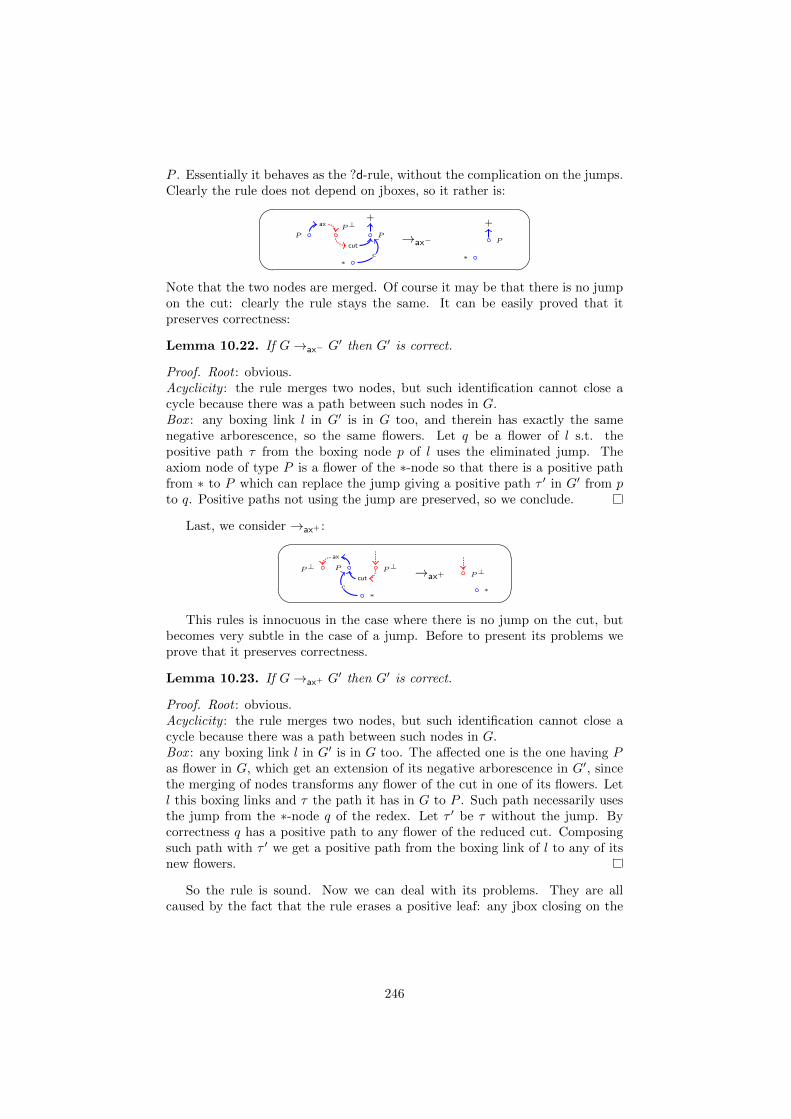
P . Essentially it behaves as the ?d-rule, without the complication on the jumps.Clearly the rule does not depend on jboxes, so it rather is:

P

+P⊥

P

ax

cut

∗c

→ax− P

+

∗

Note that the two nodes are merged. Of course it may be that there is no jumpon the cut: clearly the rule stays the same. It can be easily proved that itpreserves correctness:

Lemma 10.22. If G→ax− G′ then G′ is correct.

Proof. Root : obvious.Acyclicity : the rule merges two nodes, but such identification cannot close acycle because there was a path between such nodes in G.Box : any boxing link l in G′ is in G too, and therein has exactly the samenegative arborescence, so the same flowers. Let q be a flower of l s.t. thepositive path τ from the boxing node p of l uses the eliminated jump. Theaxiom node of type P is a flower of the ∗-node so that there is a positive pathfrom ∗ to P which can replace the jump giving a positive path τ ′ in G′ from pto q. Positive paths not using the jump are preserved, so we conclude.

Last, we consider →ax+ :

P⊥PP⊥ax

cut

∗c

→ax+ P⊥

∗

This rules is innocuous in the case where there is no jump on the cut, butbecomes very subtle in the case of a jump. Before to present its problems weprove that it preserves correctness.

Lemma 10.23. If G→ax+ G′ then G′ is correct.

Proof. Root : obvious.Acyclicity : the rule merges two nodes, but such identification cannot close acycle because there was a path between such nodes in G.Box : any boxing link l in G′ is in G too. The affected one is the one having Pas flower in G, which get an extension of its negative arborescence in G′, sincethe merging of nodes transforms any flower of the cut in one of its flowers. Letl this boxing links and τ the path it has in G to P . Such path necessarily usesthe jump from the ∗-node q of the redex. Let τ ′ be τ without the jump. Bycorrectness q has a positive path to any flower of the reduced cut. Composingsuch path with τ ′ we get a positive path from the boxing link of l to any of itsnew flowers.

So the rule is sound. Now we can deal with its problems. They are allcaused by the fact that the rule erases a positive leaf: any jbox closing on the

246

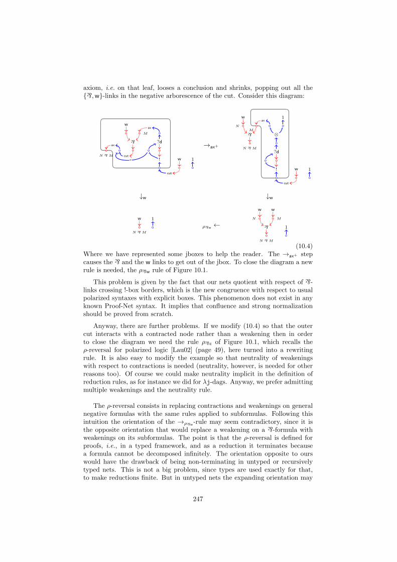
axiom, i.e. on that leaf, looses a conclusion and shrinks, popping out all the`,w-links in the negative arborescence of the cut. Consider this diagram:

M

wax

`

N `M

ax

cut!

?d

w

cut

1c

→ax+

⊗M

N

wax

1

N `M

`

!

?d

w

cut

1

↓w ↓w

N `M

w 1

ρ`w←

N

w

M

w

N `M

` 1

(10.4)Where we have represented some jboxes to help the reader. The →ax+ stepcauses the ` and the w links to get out of the jbox. To close the diagram a newrule is needed, the ρ`w rule of Figure 10.1.

This problem is given by the fact that our nets quotient with respect of `-links crossing !-box borders, which is the new congruence with respect to usualpolarized syntaxes with explicit boxes. This phenomenon does not exist in anyknown Proof-Net syntax. It implies that confluence and strong normalizationshould be proved from scratch.

Anyway, there are further problems. If we modify (10.4) so that the outercut interacts with a contracted node rather than a weakening then in orderto close the diagram we need the rule ρ`c of Figure 10.1, which recalls theρ-reversal for polarized logic [Lau02] (page 49), here turned into a rewritingrule. It is also easy to modify the example so that neutrality of weakeningswith respect to contractions is needed (neutrality, however, is needed for otherreasons too). Of course we could make neutrality implicit in the definition ofreduction rules, as for instance we did for λj-dags. Anyway, we prefer admittingmultiple weakenings and the neutrality rule.

The ρ-reversal consists in replacing contractions and weakenings on generalnegative formulas with the same rules applied to subformulas. Following thisintuition the orientation of the →ρ`w

-rule may seem contradictory, since it isthe opposite orientation that would replace a weakening on a `-formula withweakenings on its subformulas. The point is that the ρ-reversal is defined forproofs, i.e., in a typed framework, and as a reduction it terminates becausea formula cannot be decomposed infinitely. The orientation opposite to ourswould have the drawback of being non-terminating in untyped or recursivelytyped nets. This is not a big problem, since types are used exactly for that,to make reductions finite. But in untyped nets the expanding orientation may

247

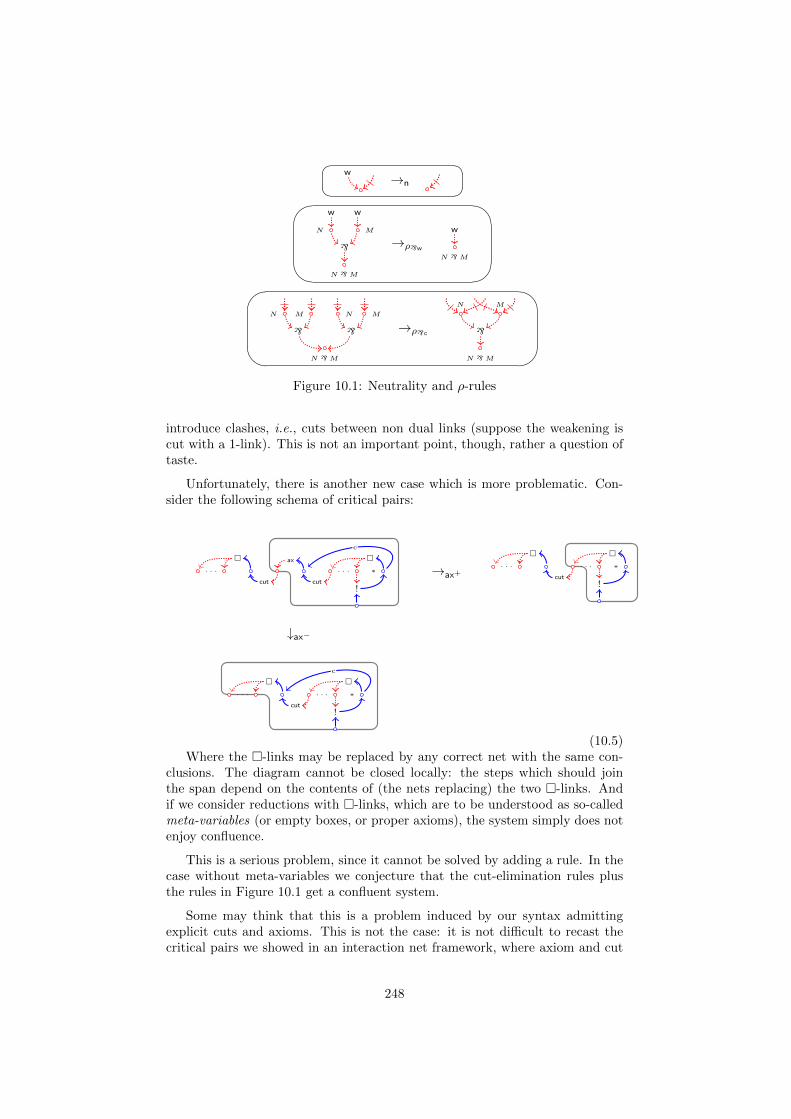
w →n

N `M

N M

`

w w

→ρ`w

N `M

w

N `M

` `

N M N M

→ρ`c

N `M

N M

`

Figure 10.1: Neutrality and ρ-rules

introduce clashes, i.e., cuts between non dual links (suppose the weakening iscut with a 1-link). This is not an important point, though, rather a question oftaste.

Unfortunately, there is another new case which is more problematic. Con-sider the following schema of critical pairs:

∗

. . .

!cut

ax

cut

. . .

c

→ax+∗

. . .

!cut

. . .

↓ax−

∗

. . .

!cut

. . .

c

(10.5)Where the -links may be replaced by any correct net with the same con-

clusions. The diagram cannot be closed locally: the steps which should jointhe span depend on the contents of (the nets replacing) the two -links. Andif we consider reductions with -links, which are to be understood as so-calledmeta-variables (or empty boxes, or proper axioms), the system simply does notenjoy confluence.

This is a serious problem, since it cannot be solved by adding a rule. In thecase without meta-variables we conjecture that the cut-elimination rules plusthe rules in Figure 10.1 get a confluent system.

Some may think that this is a problem induced by our syntax admittingexplicit cuts and axioms. This is not the case: it is not difficult to recast thecritical pairs we showed in an interaction net framework, where axiom and cut

248

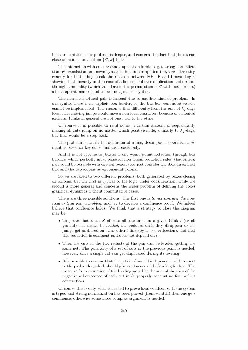
links are omitted. The problem is deeper, and concerns the fact that jboxes canclose on axioms but not on `,w-links.

The interaction with erasures and duplication forbid to get strong normaliza-tion by translation on known syntaxes, but in our opinion they are interestingexactly for that: they break the relation between MELLP and Linear Logic,showing that linearity in the sense of a fine control over duplication and erasurethrough a modality (which would avoid the permutation of ` with box borders)affects operational semantics too, not just the syntax.

The non-local critical pair is instead due to another kind of problem. Inour syntax there is no explicit box border, so the box-box commutative rulecannot be implemented. The reason is that differently from the case of λj-dagslocal rules moving jumps would have a non-local character, because of canonicalanchors: !-links in general are not one next to the other.

Of course it is possible to reintroduce a certain amount of sequentialitymaking all cuts jump on no matter which positive node, similarly to λj-dags,but that would be a step back.

The problem concerns the definition of a fine, decomposed operational se-mantics based on key cut-elimination cases only.

And it is not specific to jboxes: if one would admit reduction through boxborders, which perfectly make sense for non-axiom reduction rules, that criticalpair could be possible with explicit boxes, too: just consider the jbox an explicitbox and the two axioms as exponential axioms.

So we are faced to two different problems, both generated by boxes closingon axioms, but the first is typical of the logic under consideration, while thesecond is more general and concerns the wider problem of defining the boxesgraphical dynamics without commutative cases.

There are three possible solutions. The first one is to not consider the non-local critical pair a problem and try to develop a confluence proof. We indeedbelieve that confluence holds. We think that a strategy to close the diagrammay be:

• To prove that a set S of cuts all anchored on a given !-link l (or allground) can always be leveled, i.e., reduced until they disappear or thejumps get anchored on some other !-link (by a →?d reduction), and thatthis reduction is confluent and does not depend on l.

• Then the cuts in the two reducts of the pair can be leveled getting thesame net. The generality of a set of cuts in the previous point is needed,however, since a single cut can get duplicated during its leveling.

• It is possible to assume that the cuts in S are all independent with respectto the path order, which should give confluence of the leveling for free. Themeasure for termination of the leveling would be the sum of the sizes of thenegative arborescence of each cut in S, properly accounting for implicitcontractions.

Of course this is only what is needed to prove local confluence. If the systemis typed and strong normalization has been proved (from scratch) then one getsconfluence, otherwise some more complex argument is needed.

249

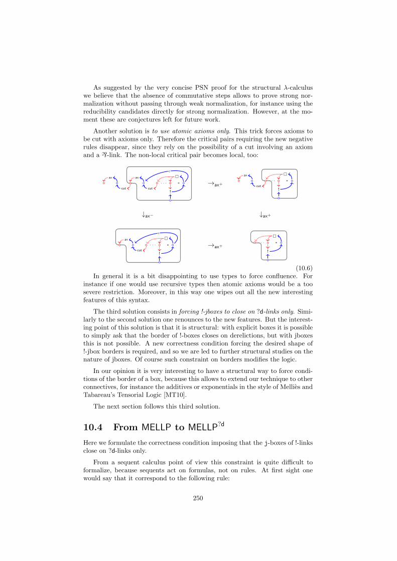
As suggested by the very concise PSN proof for the structural λ-calculuswe believe that the absence of commutative steps allows to prove strong nor-malization without passing through weak normalization, for instance using thereducibility candidates directly for strong normalization. However, at the mo-ment these are conjectures left for future work.

Another solution is to use atomic axioms only. This trick forces axioms tobe cut with axioms only. Therefore the critical pairs requiring the new negativerules disappear, since they rely on the possibility of a cut involving an axiomand a `-link. The non-local critical pair becomes local, too:

∗

. . .

!cut

ax

cut

ax

c

→ax+∗

. . .

!cut

ax

↓ax− ↓ax+

∗

. . .

!cut

ax

c

→ax+∗

. . .

!

(10.6)In general it is a bit disappointing to use types to force confluence. For

instance if one would use recursive types then atomic axioms would be a toosevere restriction. Moreover, in this way one wipes out all the new interestingfeatures of this syntax.

The third solution consists in forcing !-jboxes to close on ?d-links only. Simi-larly to the second solution one renounces to the new features. But the interest-ing point of this solution is that it is structural: with explicit boxes it is possibleto simply ask that the border of !-boxes closes on derelictions, but with jboxesthis is not possible. A new correctness condition forcing the desired shape of!-jbox borders is required, and so we are led to further structural studies on thenature of jboxes. Of course such constraint on borders modifies the logic.

In our opinion it is very interesting to have a structural way to force condi-tions of the border of a box, because this allows to extend our technique to otherconnectives, for instance the additives or exponentials in the style of Mellies andTabareau’s Tensorial Logic [MT10].

The next section follows this third solution.

10.4 From MELLP to MELLP?d

Here we formulate the correctness condition imposing that the j-boxes of !-linksclose on ?d-links only.

From a sequent calculus point of view this constraint is quite difficult toformalize, because sequents act on formulas, not on rules. At first sight onewould say that it correspond to the following rule:

250

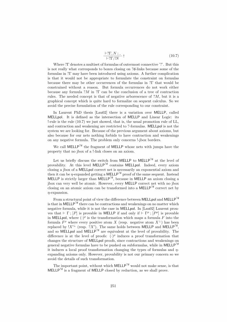
`?Γ, N ;!`?Γ; !N

(10.7)

Where ?Γ denotes a multiset of formulas of outermost connective ’?’. But thisis not really what corresponds to boxes closing on ?d-links because some of theformulas in ?Γ may have been introduced using axioms. A further complicationis that it would not be appropriate to formulate the constraint on formulasbecause there may be other occurrences of the formulas in ?Γ that would beconstrained without a reason. But formula occurrences do not work eitherbecause any formula ?M in ?Γ can be the conclusion of a tree of contractionrules. The needed concept is that of negative arborescence of ?M , but it is agraphical concept which is quite hard to formalize on sequent calculus. So weavoid the precise formulation of the rule corresponding to our constraint.

In Laurent PhD thesis [Lau02] there is a variation over MELLP, calledMELLpol. It is defined as the intersection of MELLP and Linear Logic: its!-rule is the rule (10.7) we just showed, that is, the usual promotion rule of LL,and contraction and weakening are restricted to ?-formulas. MELLpol is not thesystem we are looking for. Because of the previous argument about axioms, butalso because for our nets nothing forbids to have contraction and weakeningson any negative formula. The problem only concerns !-jbox borders.

We call MELLP?d the fragment of MELLP whose nets with jumps have theproperty that no jbox of a !-link closes on an axiom.

Let us briefly discuss the switch from MELLP to MELLP?d at the level ofprovability. At this level MELLP?d contains MELLpol. Indeed, every axiomclosing a jbox of a MELLpol correct net is necessarily an exponential axiom andthen it can be η-expanded getting a MELLP?d proof of the same sequent. InsteadMELLP is strictly larger than MELLP?d, because in MELLP an axiom closing ajbox can very well be atomic. However, every MELLP correct net with no jboxclosing on an atomic axiom can be transformed into a MELLP?d correct net byη-expansion.

From a structural point of view the difference between MELLpol and MELLP?d

is that in MELLP?d there can be contractions and weakenings on no matter whichnegative formula, while it is not the case in MELLpol. In [Lau02] Laurent prou-ves that ` Γ ; [P ] is provable in MELLP if and only if ` Γρ ; [P ρ] is provablein MELLpol, where (·)ρ is the transformation which maps a formula F into theformula F ρ where every positive atom X (resp. negative atom X⊥) has beenreplaced by !X ′⊥ (resp. ?X ′). The same holds between MELLP and MELLP?d,and so MELLpol and MELLP?d are equivalent at the level of provability. Thedifference is at the level of proofs: (·)ρ induces a proof transformation thatchanges the structure of MELLpol proofs, since contractions and weakenings ongeneral negative formulas have to be pushed on subformulas, while in MELLP?d

it induces a local proof transformation changing the types of formulas and η-expanding axioms only. However, provability is not our primary concern so weavoid the details of such transformation.

The important point, without which MELLP?d would not make sense, is thatMELLP?d is a fragment of MELLP closed by reduction, as we shall prove.

251

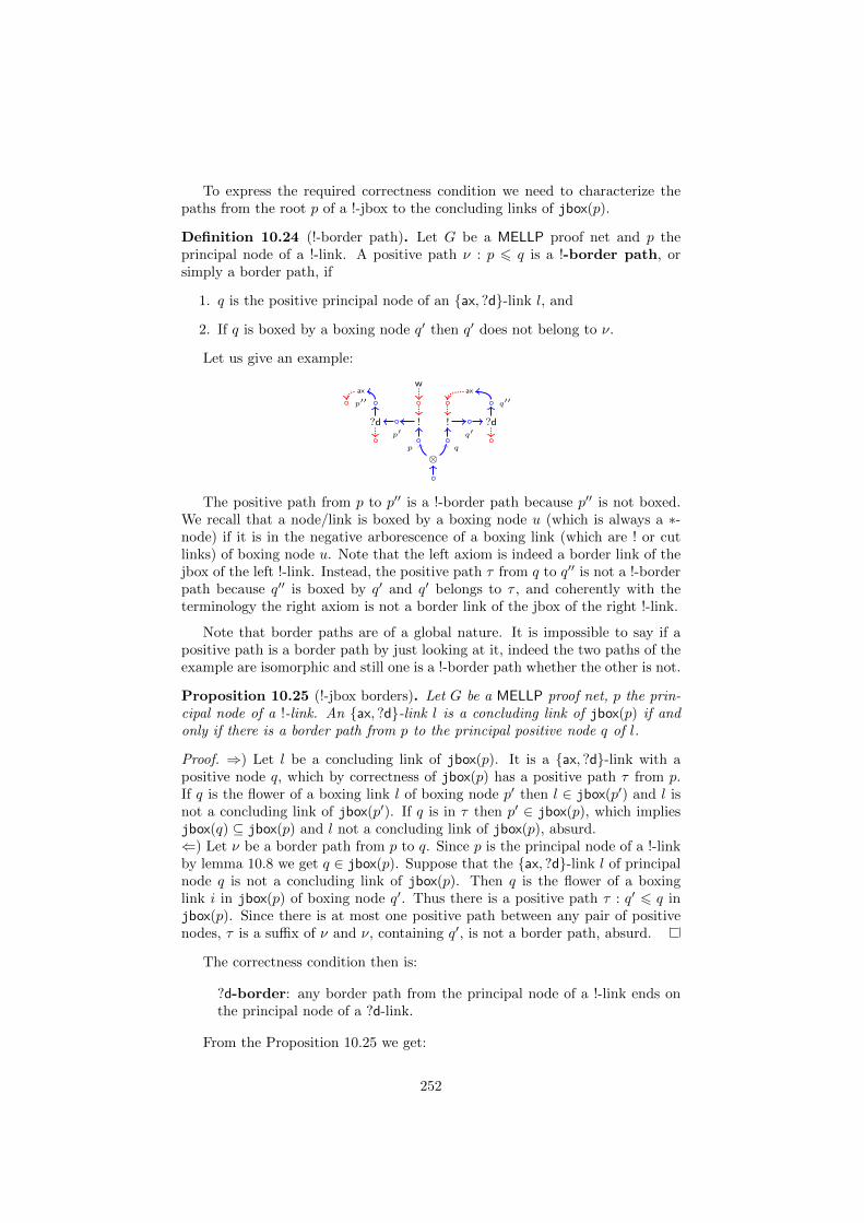
To express the required correctness condition we need to characterize thepaths from the root p of a !-jbox to the concluding links of jbox(p).

Definition 10.24 (!-border path). Let G be a MELLP proof net and p theprincipal node of a !-link. A positive path ν : p 6 q is a !-border path, orsimply a border path, if

1. q is the positive principal node of an ax, ?d-link l, and

2. If q is boxed by a boxing node q′ then q′ does not belong to ν.

Let us give an example:

p q

⊗

q′′ax

?d!q′

p′′ax

w

?d !p′

The positive path from p to p′′ is a !-border path because p′′ is not boxed.We recall that a node/link is boxed by a boxing node u (which is always a ∗-node) if it is in the negative arborescence of a boxing link (which are ! or cutlinks) of boxing node u. Note that the left axiom is indeed a border link of thejbox of the left !-link. Instead, the positive path τ from q to q′′ is not a !-borderpath because q′′ is boxed by q′ and q′ belongs to τ , and coherently with theterminology the right axiom is not a border link of the jbox of the right !-link.

Note that border paths are of a global nature. It is impossible to say if apositive path is a border path by just looking at it, indeed the two paths of theexample are isomorphic and still one is a !-border path whether the other is not.

Proposition 10.25 (!-jbox borders). Let G be a MELLP proof net, p the prin-cipal node of a !-link. An ax, ?d-link l is a concluding link of jbox(p) if andonly if there is a border path from p to the principal positive node q of l.

Proof. ⇒) Let l be a concluding link of jbox(p). It is a ax, ?d-link with apositive node q, which by correctness of jbox(p) has a positive path τ from p.If q is the flower of a boxing link l of boxing node p′ then l ∈ jbox(p′) and l isnot a concluding link of jbox(p′). If q is in τ then p′ ∈ jbox(p), which impliesjbox(q) ⊆ jbox(p) and l not a concluding link of jbox(p), absurd.⇐) Let ν be a border path from p to q. Since p is the principal node of a !-linkby lemma 10.8 we get q ∈ jbox(p). Suppose that the ax, ?d-link l of principalnode q is not a concluding link of jbox(p). Then q is the flower of a boxinglink i in jbox(p) of boxing node q′. Thus there is a positive path τ : q′ 6 q injbox(p). Since there is at most one positive path between any pair of positivenodes, τ is a suffix of ν and ν, containing q′, is not a border path, absurd.

The correctness condition then is:

?d-border: any border path from the principal node of a !-link ends onthe principal node of a ?d-link.

From the Proposition 10.25 we get:

252

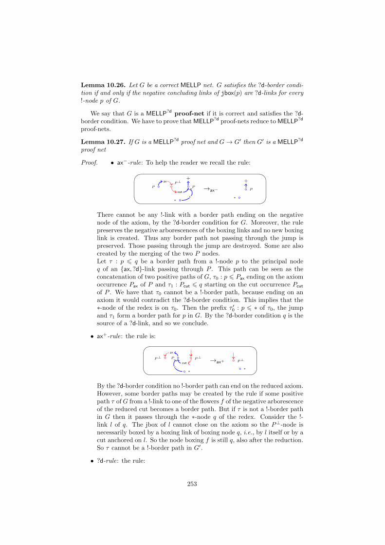
Lemma 10.26. Let G be a correct MELLP net. G satisfies the ?d-border condi-tion if and only if the negative concluding links of jbox(p) are ?d-links for every!-node p of G.

We say that G is a MELLP?d proof-net if it is correct and satisfies the ?d-border condition. We have to prove that MELLP?d proof-nets reduce to MELLP?d

proof-nets.

Lemma 10.27. If G is a MELLP?d proof net and G→ G′ then G′ is a MELLP?d

proof net

Proof. • ax−-rule: To help the reader we recall the rule:

P

+P⊥

P

ax

cut

∗c

→ax− P

+

∗

There cannot be any !-link with a border path ending on the negativenode of the axiom, by the ?d-border condition for G. Moreover, the rulepreserves the negative arborescences of the boxing links and no new boxinglink is created. Thus any border path not passing through the jump ispreserved. Those passing through the jump are destroyed. Some are alsocreated by the merging of the two P nodes.Let τ : p 6 q be a border path from a !-node p to the principal nodeq of an ax, ?d-link passing through P . This path can be seen as theconcatenation of two positive paths of G, τ0 : p 6 Pax ending on the axiomoccurrence Pax of P and τ1 : Pcut 6 q starting on the cut occurrence Pcut

of P . We have that τ0 cannot be a !-border path, because ending on anaxiom it would contradict the ?d-border condition. This implies that the∗-node of the redex is on τ0. Then the prefix τ ′0 : p 6 ∗ of τ0, the jumpand τ1 form a border path for p in G. By the ?d-border condition q is thesource of a ?d-link, and so we conclude.

• ax+-rule: the rule is:

P⊥PP⊥ax

cut

∗c

→ax+ P⊥

∗

By the ?d-border condition no !-border path can end on the reduced axiom.However, some border paths may be created by the rule if some positivepath τ ofG from a !-link to one of the flowers f of the negative arborescenceof the reduced cut becomes a border path. But if τ is not a !-border pathin G then it passes through the ∗-node q of the redex. Consider the !-link l of q. The jbox of l cannot close on the axiom so the P⊥-node isnecessarily boxed by a boxing link of boxing node q, i.e., by l itself or by acut anchored on l. So the node boxing f is still q, also after the reduction.So τ cannot be a !-border path in G′.

• ?d-rule: the rule:

253

#

"

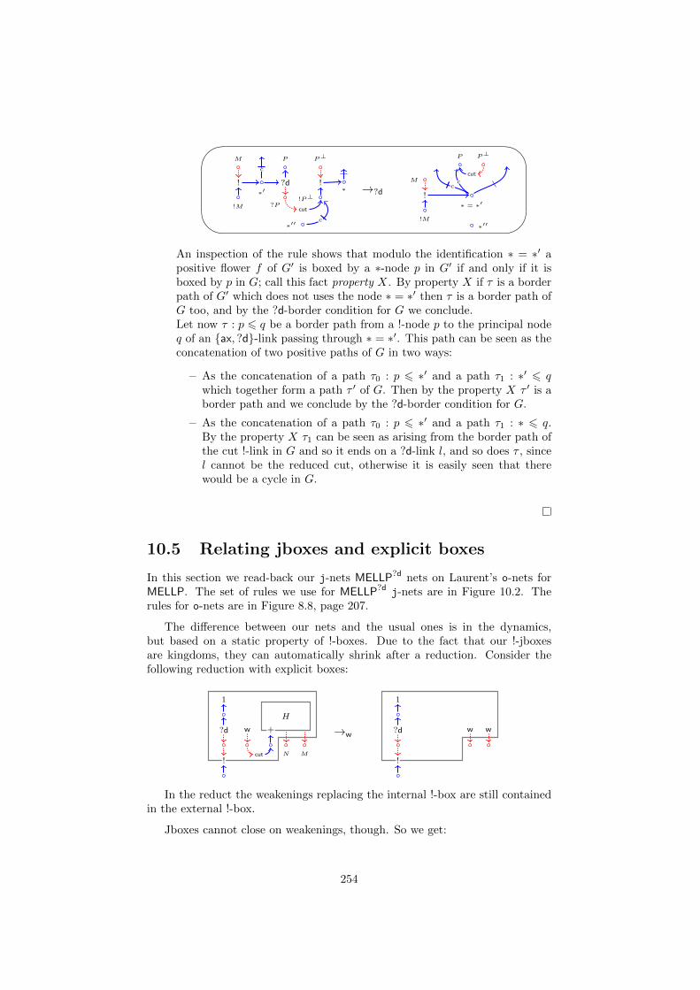
!?P

P

?d

!P⊥

P⊥

∗!

cut

∗′′c

M

!M

!∗′

c

→?d

P P⊥

cutM

!M

!∗ = ∗′

cc

∗′′

An inspection of the rule shows that modulo the identification ∗ = ∗′ apositive flower f of G′ is boxed by a ∗-node p in G′ if and only if it isboxed by p in G; call this fact property X. By property X if τ is a borderpath of G′ which does not uses the node ∗ = ∗′ then τ is a border path ofG too, and by the ?d-border condition for G we conclude.Let now τ : p 6 q be a border path from a !-node p to the principal nodeq of an ax, ?d-link passing through ∗ = ∗′. This path can be seen as theconcatenation of two positive paths of G in two ways:

– As the concatenation of a path τ0 : p 6 ∗′ and a path τ1 : ∗′ 6 qwhich together form a path τ ′ of G. Then by the property X τ ′ is aborder path and we conclude by the ?d-border condition for G.

– As the concatenation of a path τ0 : p 6 ∗′ and a path τ1 : ∗ 6 q.By the property X τ1 can be seen as arising from the border path ofthe cut !-link in G and so it ends on a ?d-link l, and so does τ , sincel cannot be the reduced cut, otherwise it is easily seen that therewould be a cycle in G.

10.5 Relating jboxes and explicit boxes

In this section we read-back our j-nets MELLP?d nets on Laurent’s o-nets forMELLP. The set of rules we use for MELLP?d j-nets are in Figure 10.2. Therules for o-nets are in Figure 8.8, page 207.

The difference between our nets and the usual ones is in the dynamics,but based on a static property of !-boxes. Due to the fact that our !-jboxesare kingdoms, they can automatically shrink after a reduction. Consider thefollowing reduction with explicit boxes:

w

1

?d +

MN

H

!cut

→w

1

?d ww

!

In the reduct the weakenings replacing the internal !-box are still containedin the external !-box.

Jboxes cannot close on weakenings, though. So we get:

254

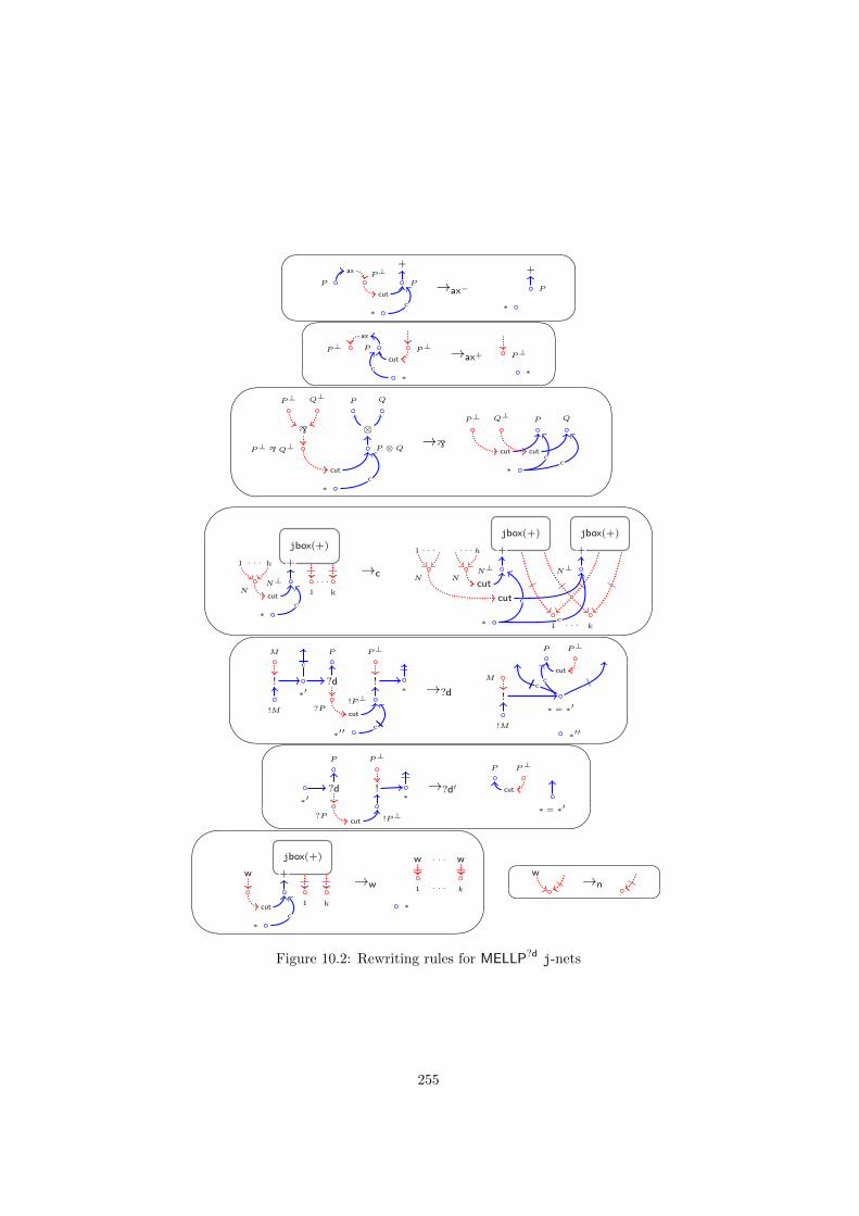
P

+P⊥

P

ax

cut

∗c

→ax− P

+

∗

P⊥PP⊥ax

cut

∗c

→ax+ P⊥

∗#

"

!P ⊗ Q

P Q

⊗

P⊥ ` Q⊥

P⊥ Q⊥

`

cut

∗c

→`

P QQ⊥P⊥

cut cut

∗

cc

'

&

$

%N

1 h. . .

N⊥

+

k1

jbox(+)

. . .

cut

∗c

→cN

1 . . .

N

h. . .

N⊥

+

jbox(+)

cut

N⊥

+

jbox(+)

1 k. . .

cut

∗

c

c#

"

!?P

P

?d

!P⊥

P⊥

∗!

cut

∗′′c

M

!M

!∗′

c

→?d

P P⊥

cutM

!M

!∗ = ∗′

cc

∗′′

?P

P

?d

!P⊥

P⊥

∗!

cut

∗′→?d′

P P⊥

cut

∗ = ∗′#

"

!w +

k1

jbox(+)

cut

∗c

→w1 k

w w. . .

. . .

∗

w →n

Figure 10.2: Rewriting rules for MELLP?d j-nets

255

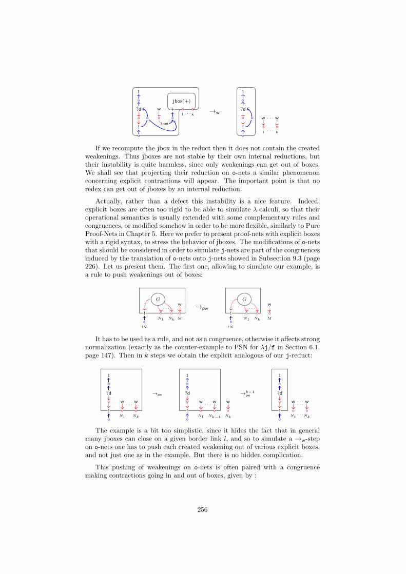
w

1

?d +k1 . . .

jbox(+)

!cut

c

→w

1

?d

!1 k

w w. . .

. . .

If we recompute the jbox in the reduct then it does not contain the createdweakenings. Thus jboxes are not stable by their own internal reductions, buttheir instability is quite harmless, since only weakenings can get out of boxes.We shall see that projecting their reduction on o-nets a similar phenomenonconcerning explicit contractions will appear. The important point is that noredex can get out of jboxes by an internal reduction.

Actually, rather than a defect this instability is a nice feature. Indeed,explicit boxes are often too rigid to be able to simulate λ-calculi, so that theiroperational semantics is usually extended with some complementary rules andcongruences, or modified somehow in order to be more flexible, similarly to PureProof-Nets in Chapter 5. Here we prefer to present proof-nets with explicit boxeswith a rigid syntax, to stress the behavior of jboxes. The modifications of o-netsthat should be considered in order to simulate j-nets are part of the congruencesinduced by the translation of o-nets onto j-nets showed in Subsection 9.3 (page226). Let us present them. The first one, allowing to simulate our example, isa rule to push weakenings out of boxes:

!N

!NkN1

. . .

G

M

w →pw

!N

!NkN1

. . .

G

M

w

It has to be used as a rule, and not as a congruence, otherwise it affects strongnormalization (exactly as the counter-example to PSN for λj/f in Section 6.1,page 147). Then in k steps we obtain the explicit analogous of our j-reduct:

1

?d

!N1 Nk

. . .w w

→pw

1

?d

!N1 Nk−1

. . .w w

Nk

w

→k−1pw

1

?d

!N1 Nk

. . .w w. . .

. . .

The example is a bit too simplistic, since it hides the fact that in generalmany jboxes can close on a given border link l, and so to simulate a →w-stepon o-nets one has to push each created weakening out of various explicit boxes,and not just one as in the example. But there is no hidden complication.

This pushing of weakenings on o-nets is often paired with a congruencemaking contractions going in and out of boxes, given by :

256

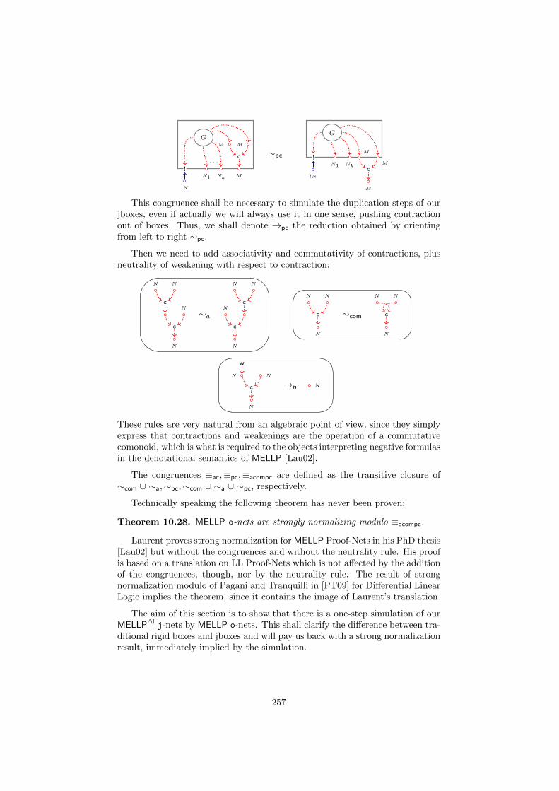
!N

!NkN1

. . .

G

M

MM

c ∼pc

!N

!NkN1

. . .

G

M

M

M

c

This congruence shall be necessary to simulate the duplication steps of ourjboxes, even if actually we will always use it in one sense, pushing contractionout of boxes. Thus, we shall denote →pc the reduction obtained by orientingfrom left to right ∼pc.

Then we need to add associativity and commutativity of contractions, plusneutrality of weakening with respect to contraction:'

&

$

%

N N

cN

N

c

∼a

N N

cN

N

c

N N

N

c ∼com

N N

N

c

N

w

N

N

c →n N

These rules are very natural from an algebraic point of view, since they simplyexpress that contractions and weakenings are the operation of a commutativecomonoid, which is what is required to the objects interpreting negative formulasin the denotational semantics of MELLP [Lau02].

The congruences ≡ac,≡pc,≡acompc are defined as the transitive closure of∼com ∪ ∼a,∼pc,∼com ∪ ∼a ∪ ∼pc, respectively.

Technically speaking the following theorem has never been proven:

Theorem 10.28. MELLP o-nets are strongly normalizing modulo ≡acompc.

Laurent proves strong normalization for MELLP Proof-Nets in his PhD thesis[Lau02] but without the congruences and without the neutrality rule. His proofis based on a translation on LL Proof-Nets which is not affected by the additionof the congruences, though, nor by the neutrality rule. The result of strongnormalization modulo of Pagani and Tranquilli in [PT09] for Differential LinearLogic implies the theorem, since it contains the image of Laurent’s translation.

The aim of this section is to show that there is a one-step simulation of ourMELLP?d j-nets by MELLP o-nets. This shall clarify the difference between tra-ditional rigid boxes and jboxes and will pay us back with a strong normalizationresult, immediately implied by the simulation.

257

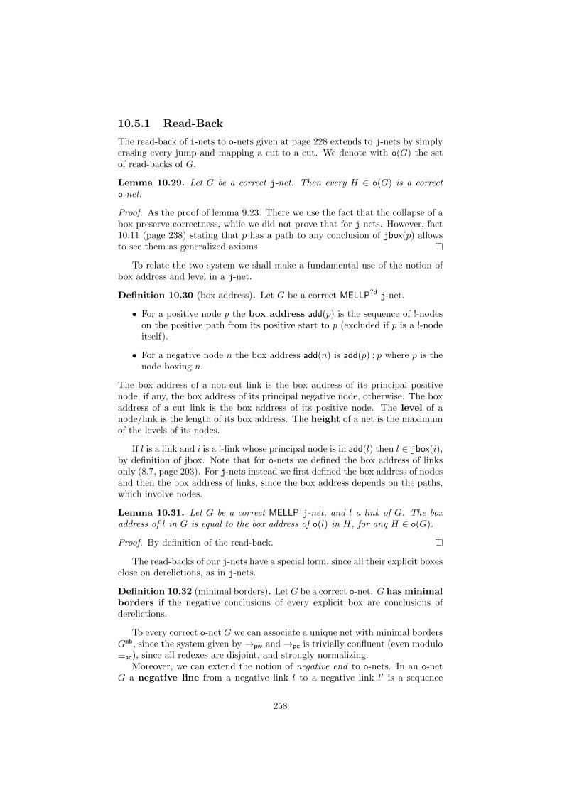
10.5.1 Read-Back

The read-back of i-nets to o-nets given at page 228 extends to j-nets by simplyerasing every jump and mapping a cut to a cut. We denote with o(G) the setof read-backs of G.

Lemma 10.29. Let G be a correct j-net. Then every H ∈ o(G) is a correcto-net.

Proof. As the proof of lemma 9.23. There we use the fact that the collapse of abox preserve correctness, while we did not prove that for j-nets. However, fact10.11 (page 238) stating that p has a path to any conclusion of jbox(p) allowsto see them as generalized axioms.

To relate the two system we shall make a fundamental use of the notion ofbox address and level in a j-net.

Definition 10.30 (box address). Let G be a correct MELLP?d j-net.

• For a positive node p the box address add(p) is the sequence of !-nodeson the positive path from its positive start to p (excluded if p is a !-nodeitself).

• For a negative node n the box address add(n) is add(p) ; p where p is thenode boxing n.

The box address of a non-cut link is the box address of its principal positivenode, if any, the box address of its principal negative node, otherwise. The boxaddress of a cut link is the box address of its positive node. The level of anode/link is the length of its box address. The height of a net is the maximumof the levels of its nodes.

If l is a link and i is a !-link whose principal node is in add(l) then l ∈ jbox(i),by definition of jbox. Note that for o-nets we defined the box address of linksonly (8.7, page 203). For j-nets instead we first defined the box address of nodesand then the box address of links, since the box address depends on the paths,which involve nodes.

Lemma 10.31. Let G be a correct MELLP j-net, and l a link of G. The boxaddress of l in G is equal to the box address of o(l) in H, for any H ∈ o(G).

Proof. By definition of the read-back.

The read-backs of our j-nets have a special form, since all their explicit boxesclose on derelictions, as in j-nets.

Definition 10.32 (minimal borders). LetG be a correct o-net. G has minimalborders if the negative conclusions of every explicit box are conclusions ofderelictions.

To every correct o-net G we can associate a unique net with minimal bordersGmb, since the system given by→pw and→pc is trivially confluent (even modulo≡ac), since all redexes are disjoint, and strongly normalizing.

Moreover, we can extend the notion of negative end to o-nets. In an o-netG a negative line from a negative link l to a negative link l′ is a sequence

258

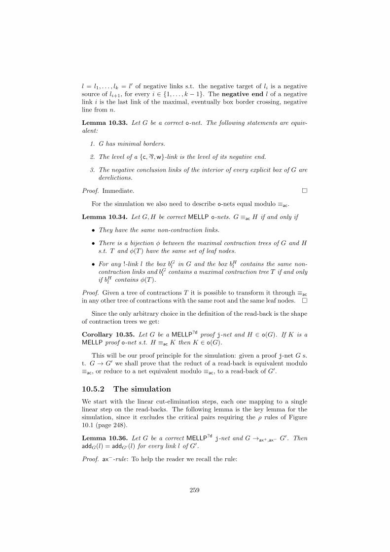
l = l1, . . . , lk = l′ of negative links s.t. the negative target of li is a negativesource of li+1, for every i ∈ 1, . . . , k − 1. The negative end l of a negativelink i is the last link of the maximal, eventually box border crossing, negativeline from n.

Lemma 10.33. Let G be a correct o-net. The following statements are equiv-alent:

1. G has minimal borders.

2. The level of a c,`,w-link is the level of its negative end.

3. The negative conclusion links of the interior of every explicit box of G arederelictions.

Proof. Immediate.

For the simulation we also need to describe o-nets equal modulo ≡ac.

Lemma 10.34. Let G,H be correct MELLP o-nets. G ≡ac H if and only if

• They have the same non-contraction links.

• There is a bijection φ between the maximal contraction trees of G and Hs.t. T and φ(T ) have the same set of leaf nodes.

• For any !-link l the box bGl in G and the box bHl contains the same non-contraction links and bGl contains a maximal contraction tree T if and onlyif bHl contains φ(T ).

Proof. Given a tree of contractions T it is possible to transform it through ≡ac

in any other tree of contractions with the same root and the same leaf nodes.

Since the only arbitrary choice in the definition of the read-back is the shapeof contraction trees we get:

Corollary 10.35. Let G be a MELLP?d proof j-net and H ∈ o(G). If K is aMELLP proof o-net s.t. H ≡ac K then K ∈ o(G).

This will be our proof principle for the simulation: given a proof j-net G s.t. G → G′ we shall prove that the reduct of a read-back is equivalent modulo≡ac, or reduce to a net equivalent modulo ≡ac, to a read-back of G′.

10.5.2 The simulation

We start with the linear cut-elimination steps, each one mapping to a singlelinear step on the read-backs. The following lemma is the key lemma for thesimulation, since it excludes the critical pairs requiring the ρ rules of Figure10.1 (page 248).

Lemma 10.36. Let G be a correct MELLP?d j-net and G →ax+,ax− G′. Then

addG(l) = addG′(l) for every link l of G′.

Proof. ax−-rule: To help the reader we recall the rule:

259

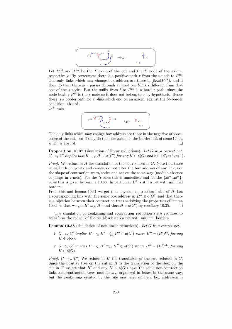
P

+P⊥

P

ax

cut

∗c

→ax− P

+

∗

Let P cut and P ax be the P node of the cut and the P node of the axiom,respectively. By correctness there is a positive path τ from the ∗-node to P ax.The only links which may change box address are those in jbox(P cut), and ifthey do then there is τ passes through at least one !-link l different from thatone of the ∗-node. But the suffix from l to P ax is a border path, since thenode boxing P ax is the ∗ node so it does not belong to τ by hypothesis. Hencethere is a border path for a !-link which end on an axiom, against the ?d-bordercondition, absurd.ax+-rule:

P⊥PP⊥ax

cut

∗c

→ax+ P⊥

∗

The only links which may change box address are those in the negative arbores-cence of the cut, but if they do then the axiom is the border link of some !-link,which is absurd.

Proposition 10.37 (simulation of linear reductions). Let G be a correct net.G→x G

′ implies that H →x H′ ∈ o(G′) for any H ∈ o(G) and x ∈ `, ax+, ax−.

Proof. We reduce in H the translation of the cut reduced in G. Note that theserules, both on j-nets and o-nets, do not alter the box address of any link, northe shape of contraction trees/nodes and act on the same way (modulo absenceof jumps in o-nets). For the `-rules this is immediate and for the ax−, ax+-rules this is given by lemma 10.36. In particular H ′ is still a net with minimalborders.From this and lemma 10.31 we get that any non-contraction link l of H ′ hasa corresponding link with the same box address in H ′′ ∈ o(G′) and that thereis a bijection between their contraction trees satisfying the properties of lemma10.34 so that we get H ′ ≡ac H

′′ and thus H ∈ o(G′) by corollary 10.35.

The simulation of weakening and contraction reduction steps requires totransform the reduct of the read-back into a net with minimal borders.

Lemma 10.38 (simulation of non-linear reductions). Let G be a correct net.

1. G→w G′ implies H →w H

′ →∗pw H ′′ ∈ o(G′) where H ′′ = (H ′)mb, for anyH ∈ o(G).

2. G →c G′ implies H →c H

′ ≡pc H′′ ∈ o(G′) where H ′′ = (H ′)mb, for any

H ∈ o(G).

Proof. G →w G′) We reduce in H the translation of the cut reduced in G.Since the positive tree on the cut in H is the translation of the jbox on thecut in G we get that H ′ and any K ∈ o(G′) have the same non-contractionlinks and contraction trees modulo ≡ac organized in boxes in the same way,but the weakenings created by the rule may have different box addresses in

260

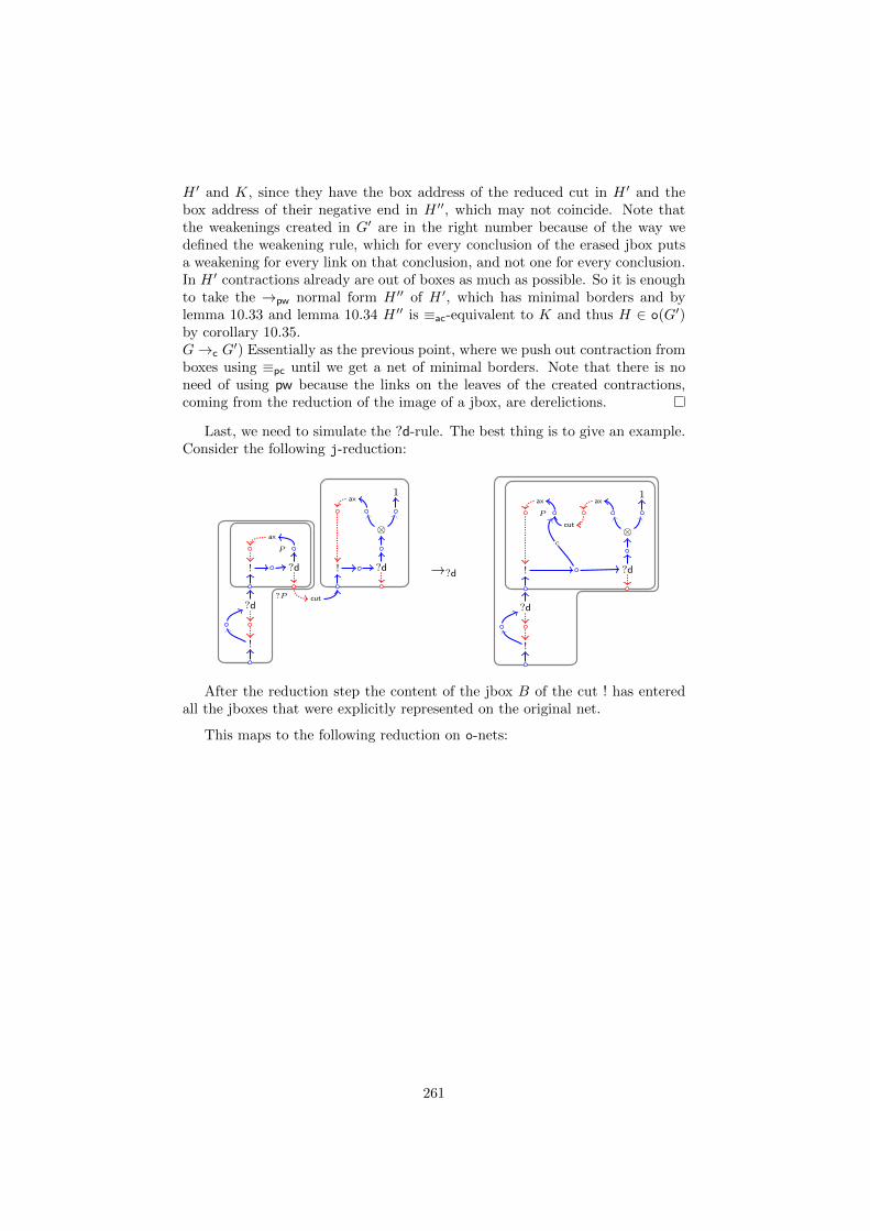
H ′ and K, since they have the box address of the reduced cut in H ′ and thebox address of their negative end in H ′′, which may not coincide. Note thatthe weakenings created in G′ are in the right number because of the way wedefined the weakening rule, which for every conclusion of the erased jbox putsa weakening for every link on that conclusion, and not one for every conclusion.In H ′ contractions already are out of boxes as much as possible. So it is enoughto take the →pw normal form H ′′ of H ′, which has minimal borders and bylemma 10.33 and lemma 10.34 H ′′ is ≡ac-equivalent to K and thus H ∈ o(G′)by corollary 10.35.G→c G

′) Essentially as the previous point, where we push out contraction fromboxes using ≡pc until we get a net of minimal borders. Note that there is noneed of using pw because the links on the leaves of the created contractions,coming from the reduction of the image of a jbox, are derelictions.

Last, we need to simulate the ?d-rule. The best thing is to give an example.Consider the following j-reduction:

P

ax

?P

! ?d

!

?dcut

?d

⊗

1ax

! →?d

P

ax ax

cut

1

⊗

! ?d

!

?d

c

After the reduction step the content of the jbox B of the cut ! has enteredall the jboxes that were explicitly represented on the original net.

This maps to the following reduction on o-nets:

261

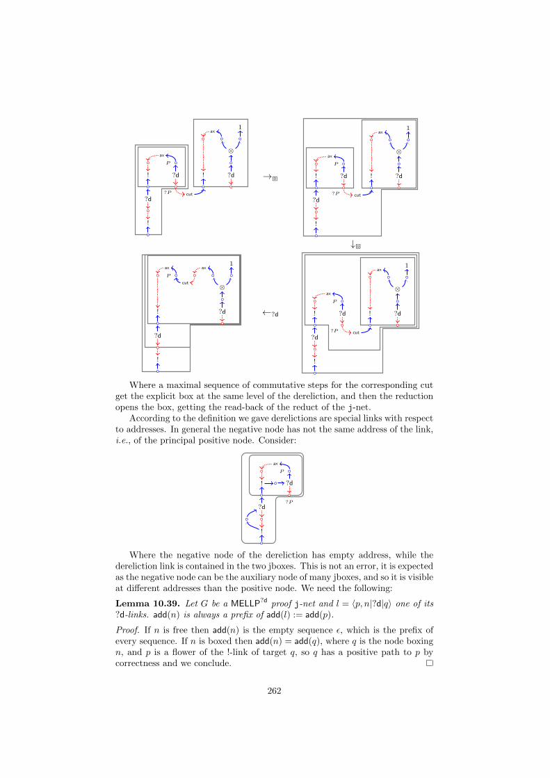
P

ax

?P

! ?d

!

?dcut

?d

⊗

1ax

! →

P

ax

?P

! ?d

!

?dcut

?d

⊗

1ax

!

↓

P

ax ax

cut

1

⊗

! ?d

!

?d

←?d

P

ax

?P

! ?d

!

?dcut

?d

⊗

1ax

!

Where a maximal sequence of commutative steps for the corresponding cutget the explicit box at the same level of the dereliction, and then the reductionopens the box, getting the read-back of the reduct of the j-net.

According to the definition we gave derelictions are special links with respectto addresses. In general the negative node has not the same address of the link,i.e., of the principal positive node. Consider:

P

ax

?P

! ?d

!

?d

Where the negative node of the dereliction has empty address, while thedereliction link is contained in the two jboxes. This is not an error, it is expectedas the negative node can be the auxiliary node of many jboxes, and so it is visibleat different addresses than the positive node. We need the following:

Lemma 10.39. Let G be a MELLP?d proof j-net and l = 〈p, n|?d|q〉 one of its?d-links. add(n) is always a prefix of add(l) := add(p).

Proof. If n is free then add(n) is the empty sequence ε, which is the prefix ofevery sequence. If n is boxed then add(n) = add(q), where q is the node boxingn, and p is a flower of the !-link of target q, so q has a positive path to p bycorrectness and we conclude.

262

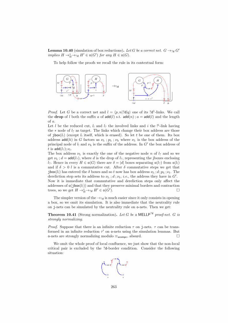
Lemma 10.40 (simulation of box reductions). Let G be a correct net. G→?d G′

implies H →∗→?d H′ ∈ o(G′) for any H ∈ o(G).

To help follow the proofs we recall the rule in its contextual form:

?P

P

∗′?d

!P⊥

P⊥

∗!

cut

M

!M

!

Γ

HG

∆

...

→?dP

P⊥

cutM

!M

!∗ = ∗′

c

G

Γ ∆

...

H

Proof. Let G be a correct net and l = 〈p, n|?d|q〉 one of its ?di-links. We callthe drop of l both the suffix a of add(l) s.t. add(n) ; a = add(l) and the lengthof a.Let l be the reduced cut, l! and l? the involved links and i the !i-link havingthe ∗ node of l? as target. The links which change their box address are thoseof jbox(l!) (except l! itself, which is erased). So let t be one of them. Its boxaddress add(h) in G factors as νl! ; pl! ; νh where νl! is the box address of theprincipal node of l! and νh is the suffix of the address. In G′ the box address oft is add(l?); νt.The box address νl! is exactly the one of the negative node n of l? and so weget νl! ; d = add(l?), where d is the drop of l?, representing the jboxes enclosingl?. Hence in every H ∈ o(G) there are δ = |d| boxes separating o(l?) from o(l!)and if δ > 0 l is a commutative cut. After δ commutative steps we get thatjbox(l!) has entered the δ boxes and so t now has box address νl! ;d ;pl! ;νt. Thedereliction step sets its address to νl! ; d ; νt, i.e., the address they have in G′.Now it is immediate that commutative and dereliction steps only affect theaddresses of o(jbox(l!)) and that they preserve minimal borders and contractiontrees, so we get H →∗→?d H

′ ∈ o(G′).

The simpler version of the→?d is much easier since it only consists in openinga box, so we omit its simulation. It is also immediate that the neutrality ruleon j-nets can be simulated by the neutrality rule on o-nets. Then we get:

Theorem 10.41 (Strong normalization). Let G be a MELLP?d proof-net. G isstrongly normalizing.

Proof. Suppose that there is an infinite reduction τ on j-nets. τ can be trans-formed in an infinite reduction τ ′ on o-nets using the simulation lemmas. Buto-nets are strongly normalizing modulo ≡acompc, absurd.

We omit the whole proof of local confluence, we just show that the non-localcritical pair is excluded by the ?d-border condition. Consider the followingsituation:

cut

ax

cut

∗ ∗

cc

263

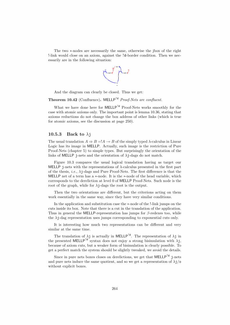
The two ∗-nodes are necessarily the same, otherwise the jbox of the right!-link would close on an axiom, against the ?d-border condition. Then we nec-essarily are in the following situation:

cut

ax

cut

∗

c

c

And the diagram can clearly be closed. Thus we get:

Theorem 10.42 (Confluence). MELLP?d Proof-Nets are confluent.

What we have done here for MELLP?d Proof-Nets works smoothly for thecase with atomic axioms only. The important point is lemma 10.36, stating thataxioms reductions do not change the box address of other links (which is truefor atomic axioms, see the discussion at page 250).

10.5.3 Back to λj

The usual translation A⇒ B =!A( B of the simply typed λ-calculus in LinearLogic has its image in MELLP. Actually, such image is the restriction of PureProof-Nets (chapter 5) to simple types. But surprisingly the orientation of thelinks of MELLP j-nets and the orientation of λj-dags do not match.

Figure 10.3 compares the usual logical translation having as target ourMELLP j-nets with the representations of λ-calculus presented in the first partof the thesis, i.e., λj-dags and Pure Proof-Nets. The first difference is that theMELLP net of a term has a ∗-node. It is the ∗-node of the head variable, whichcorresponds to the dereliction at level 0 of MELLP Proof-Nets. Such node is theroot of the graph, while for λj-dags the root is the output.

Then the two orientations are different, but the criterions acting on themwork essentially in the same way, since they have very similar conditions.

In the application and substitution case the ∗-node of the !-link jumps on thecuts inside its box. Note that there is a cut in the translation of the application.Thus in general the MELLP-representation has jumps for β-redexes too, whilethe λj-dag representation uses jumps corresponding to exponential cuts only.

It is interesting how much two representations can be different and verysimilar at the same time.

The translation of λj is actually in MELLP?d. The representation of λj inthe presented MELLP?d syntax does not enjoy a strong bisimulation with λj,because of axiom cuts, but a weaker form of bisimulation is clearly possible. Toget a perfect match the system should be slightly tweaked, we avoid the details.

Since in pure nets boxes closes on derelictions, we get that MELLP?d j-netsand pure nets induce the same quotient, and so we get a representation of λj/owithout explicit boxes.

264

'

&

$

%

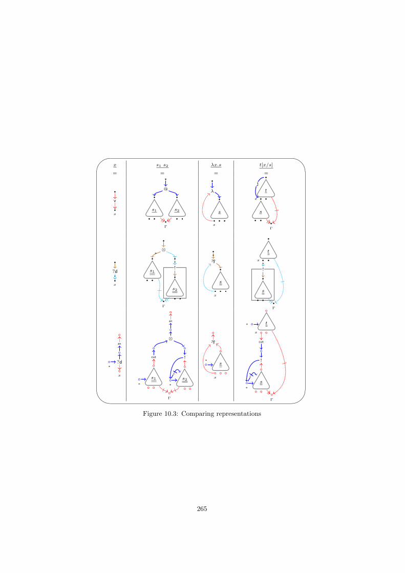
x s1 s2 λx.s t[x/s]

= = = =

x

v

@

s2s1

Γ

s

x

λ t

x

s

Γ

j

x

?d*

⊗*

!*

s2

s1

Γ

s

x

`*

t

x

!*

s

Γ

x

?d∗

ax

ax

⊗

!

s2∗

c

cut

s1∗

Γ

s

x

`

∗

t∗

x

cut

!

s∗

c

Γ

Figure 10.3: Comparing representations

265

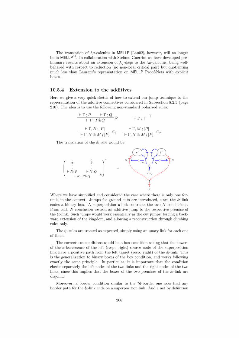
The translation of λµ-calculus in MELLP [Lau02], however, will no longerbe in MELLP?d. In collaboration with Stefano Guerrini we have developed pre-liminary results about an extension of λj-dags to the λµ-calculus, being well-behaved with respect to reduction (no non-local critical pair) but quotientingmuch less than Laurent’s representation on MELLP Proof-Nets with explicitboxes.

10.5.4 Extension to the additives

Here we give a very quick sketch of how to extend our jump technique to therepresentation of the additive connectives considered in Subsection 8.2.5 (page210). The idea is to use the following non-standard polarized rules:

` Γ ; P ` Γ ;Q&` Γ ; P&Q

>` Γ ;>

` Γ, N ; [P ]⊕l` Γ, N ⊕M ; [P ]

` Γ,M ; [P ]⊕r` Γ, N ⊕M ; [P ]

The translation of the & rule would be:

.π..

` N ;P

.

θ..

` N ;Q&` N ; P&Q

?

=

π?

NP

θ?

NQ

P&Q

N

s

&

j j

c c

Where we have simplified and considered the case where there is only one for-mula in the context. Jumps for ground cuts are introduced, since the &-linkcodes a binary box. A superposition s-link contracts the two N conclusions.From each N conclusion we add an additive jump to the respective premise ofthe &-link. Such jumps would work essentially as the cut jumps, forcing a back-ward extension of the kingdom, and allowing a reconstruction through climbingrules only.

The ⊕-rules are treated as expected, simply using an unary link for each oneof them.

The correctness conditions would be a box condition asking that the flowersof the arborescence of the left (resp. right) source node of the superpositionlink have a positive path from the left target (resp. right) of the &-link. Thisis the generalization to binary boxes of the box condition, and works followingexactly the same principle. In particular, it is important that the conditionchecks separately the left nodes of the two links and the right nodes of the twolinks, since this implies that the boxes of the two premises of the &-link aredisjoint.

Moreover, a border condition similar to the ?d-border one asks that anyborder path for the &-link ends on a superposition link. And a net by definition

266

must have a jump on every source of a superposition link, both anchored on thesame &-link. The technology for MELLP?d works smoothly.

The advantages of this representation are:

• The permutations between & and ⊗ are avoided, since they are bothpositive,

• Any cut can be eliminated, since the duplications required by superposi-tions always concerns positive links.

• Any proof maps to one net only.

• Differently from Hughes and van Glabbeek solution [HvG05] it does notdepend on types.

• Differently from slices [Gir87, LTdF04] it does not require a number oflinks exponential in the number of the rules of the corresponding proof.

It has to be said that our idea would just get a representation with boxes, withthe important difference, however, that the boxes would be implicit and locallyreconstructable. However, a more detailed study of all this is left for futurework.

267

Chapter 11

Conclusions andperspectives

This thesis contains two main achievements:

1. Implicit boxes and polarity: we developed a technique to replace theuse of explicit boxes in graphical syntaxes with a notion of local implicitbox, reconstructable in linear time and induced by the structure of thesyntactic object itself. The use of a correctness criterion gives to ourtechnique a solid status. A new understanding of logical polarity as astructural geometrical property inducing implicit boxes has also emerged.We believe that a step towards the understanding of graphical, causallocality has been made.

2. The structural λ-calculus: a new theory of explicit substitutions, thestructural λ-calculus, has been introduced and studied. It enjoys all therequired properties, with compact proofs and with no need of congruences,it has few rules, its extensions with composition and decomposition of sub-stitutions are still well-behaved, and it has a strong justification in termsof graphical syntaxes. More than a theory of explicit substitution it canbe considered a Linear Logic theory of λ-calculus, since there is a strongrelation with Pure Proof-Nets. It enjoys many operational properties andit is an useful tool to study λ-calculus and revisit existing notions undera new perspective. Essentially, it is as expressive as Pure Proof-Nets andeasier to manage.

11.1 Implicit boxes and polarity

Through our study we believe of having found some principles on the logicalfeatures leading to implicit boxes.

Our analysis of subnets in Multiplicative Linear Logic seems to shows thatthere is no hope for a local description of an implicit box in a setting where con-nectives can freely mix. Of course it may very well be that some new graphicaltechnology will change the situation, but we are skeptical about that.

268

The main problem of Multiplicative Linear Logic is that it lacks the structureto support additional layers of information, since jumps cannot be transportedby reduction. This is a serious obstacle, and our point of view is that MLLshould be taken as a beautiful an yet degenerate example of graphical language,not as a paradigm.

It seems inevitable that there are some nodes of a graph, more equal thanothers, admitting implicit boxes, and some which does not. If all nodes areconsidered to be created equally then it seems that there is no chance of buildinga box locally. To get implicit boxes one has to take from some and give to others.Hence a notion of polarity on nodes is induced by local boxability.

Such form of polarity coincide with the polarity in use in MELLP. Beinglocally boxable corresponds to being positive, and dually being not locally box-able corresponds to being negative. This suggests a new look to logical rules:some build boxes (the positive ones) and the others (the negative ones) definethe actions on them. Not surprisingly, the positive rules should follow a rigid,almost sequential discipline, to induce the skeleton tree inducing boxes, whilethe negative constructs are essentially free to float.

Polarized systems are usually conceived as being very rigid in the way theybuild proofs, when compared to non-polarized ones. Here we re-understandpolarity as a syntactic discipline forcing the local definability of implicit boxes.The constraints that polarized systems use to build a proof code into the proofstructure itself the amount of sequential information that, when switching tographs and causal locality, is necessary to obtain an implicit notion of box.

The polarity induced by local boxability and polarity as in Polarized LinearLogic coincide on MELLP, but we had point out an interesting mismatch con-cerning additive connectives. The usual polarity for the additives (& negativeand ⊕ positive) induces the need of boxes for negative formulas. But the nega-tive formulas do not enjoy locally definable implicit boxes, so a problem arises.In this thesis said mismatch is only touched on: there is more research to bedone still.

Let us conclude stating that switching the polarities of the two connectives(thus having ⊕ negative and & positive) solves the problem of the additivesand suggests that the polarity of implicit boxes groups together connectives of aconjunctive nature (!, ⊗ and &) and connectives of a disjunctive nature (⊕, `,?). This is easily understood by looking at the respective rules: the conjunctiveones are those more demanding from a graphical point of view, requiring thepossibility of splitting the net (⊗ and &) or conditions concerning their context(! and &), while the dual set of rules is generally easier to deal with1.

However, the switch of polarities affects the logic deeply, for instance itbreaks the distributivity law of the additives on the multiplicative connectives.On the other hand, a positive & and a negative ⊕ can be found in IntuitionisticLinear Logic, if one consider the right conclusion as being positive, and dually

1The 0-ary rules of weakening and ⊥ are problematic and belongs to the disjunctive set.In subsection 8.1.4 (page 196) we have pointed out to a result of Regnier showing that theproblems given by 0-ary rules are essentially due to the interaction they have with the tensorrule. From this point of view it is not necessarily true that 0-ary rules are problematic: it canbe argued that the difficulty is to handle the conjunctive rules in presence of 0-ary rules.

269

the left of the sequent as being negative. The full understanding of this problemis left for future work.

11.2 The structural λ-calculus

The study of λj-dags and the structural λ-calculus has originated by the ideathat the sequentialization theorem can be used to extract a sequential languagefrom a graphical one, by pulling the graphical operational semantics back onterms.

Then three operational concepts have emerged from our study.

The importance of establishing the relation between a graphical formalismand a calculus as a strong bisimulation, which implies a clean, simple and pow-erful operational theory, with immediate transfer of properties between the twosettings.

The absence of commutative reductions gets a sort of exponential speed-up in the length of normalization proofs, and this distinction does not rely onthe granularity of the reduction: it is possible to have small-steps operationalsemantics and key cut-elimination cases only.

The concept of distance rule, arising by the sequentialization of graphicalreduction rules, turned out to be versatile, useful and easy to deal with. Se-quential locality is misleading, and it is not necessary to use a graph formalismin order to turn towards causal locality, despite graphs certainly helps.

The operational relevance of these concepts has emerged slowly, after twoyears of research. They force a new approach, a new syntactical perspective.At first we were not sure that the structural λ-calculus was an interesting tool.Then good properties kept emerging at a surprising rate. We believe that wehave only scratched the surface.

11.3 Future work

In our opinion there is a wide range of research directions opening up. Theconcrete ones, which are extensions of the work of the thesis are:

• Extensions of implicit boxes:

– We believe that our technique for MELLP can be extended to encom-pass the whole of Second-Order Intuitionistic Linear Logic. Othersystems are also challenging: how to represent the rewriting rulesof Differential Linear Logic? Actually there is only one problematicrule, the interaction between codereliction and the auxiliary port ofa !-box. This rule poses serious obstacles, since it requires to knowthe boxes surrounding a given box. Can jumps be used to refine ourrepresentation and catch this rule?

– In collaboration with Stefano Guerrini we have preliminary results onan extension of λj-dags to the λµ-calculus which is does not match

270

the graphical representation of λµ obtained through the translationinto MELLP Proof-Nets, similarly to the mismatch between λj-dagsand the translation of λj into MELLP shown in Subsection 10.5.3(page 264).

– The experimental syntax of Chapter 7 should be better understood,and related to λj/f. That framework is a box-free representation,which is fascinating because it does not depend on a box assign-ment. For instance, both the sharing graph implementation of λ-calculu/Linear Logic and the geometry of interaction depend on thebox assignment. Can this phenomenon be useful in implementations?The behavior of that system is out of the scope of every abstract the-ory of rewriting we know of. It seems that a similar minimal use ofjumps can be done on MELLP nets too, attaching jumps on weaken-ings instead of cuts, but the development is far from being easy: newconfluence problems arise. With respect to the other possible futureworks this is certainly the most difficult and challenging.

• Sequentialization: the operational pull-back at the origin of λj can beapplied to other frameworks, too. We think in particular of term graphrewriting, where graphs are used to exploit sharing. Exactly how we havealgebrized λj-dags it is possible to algebrize term graph rewriting andobtain a new tool. In particular, term graph rewriting is often presentedas rewriting without binders, while the sharing used at the graphical levelis no more than explicit substitutions for first order rewriting.

• PSN for λj/f: we have spent a lot of time trying to prove the PSNproperty for λj/f, without success. This is important because it wouldjustify the experimental syntax of Chapter 7. Probably some further deepoperational concept is needed, in order to tame such a wild system.

• Higher-Order : it is natural to test the solidity of our approach to explicitsubstitutions by trying to use it in the context of higher-order rewriting.While the definition is straightforward, the delicate point is the proof ofPSN. Unfortunately, the proof we used for λj does not scale up to thehigher-order framework because it relies on an inductive description ofstrongly normalizing λ-terms, while for general higher-order systems sucha description is not available. A first step in this direction would be tofind a proof of PSN for λj which does not depend on such description.

• Standardization for λj and linear head reduction: we would like to tryto revisit standardization for the λ-calculus through λj. In particular wewould like to obtain a standardization theorem s.t. a standard reductionto normal form is an appropriate generalization of linear head reduction(since linear head reduction does not reduce to normal form).

• Relation of λj with traditional ES-calculi : it would be interesting to un-derstand the relation between λj and λx, at the operational level. Themain point is how to simulate in λj the following λx rule:

(t v)[x/u] →@ t[x/u] v[x/u]

271

In general this is impossible, since this rule does not depend on multiplic-ities. But there is a refinement of λx which can be probably be relatedto λj. The idea is to replace explicit substitutions [x/u] with a notion ofexplicit substitution with address [x/u]a, like in [BLR96], and to ask thatany two substitutions sharing the same address, say [x/u]a and [y/v]a,share the content too, i.e. u = v. Then it is possible to re-interpret the→@-rule as a duplication of addresses, i.e., of pointers, and not as anactual duplication of u:

(t v)[x/u]a →@′ t[x/u]a v[x/u]a

Interestingly, this is exactly how actual implementations of abstract ma-chines work (see [Lan07]): the duplication of environments present in someof their rules is implemented by duplicating the pointer to the environ-ment and not duplicating the environment.A new form of sharing is at work here. The point is that it seems to bepossible to define a projection relation form λx plus addresses to λj, whichprojects all the substitutions with the same address on the same substi-tution without address of λj, which extends to an operational projection.Nicely, we have preliminary results showing that addresses are a gener-alization of jumps: any occurrence of a substitution [x/u]a of address acan be graphically represented as a jump to the same graphical substi-tution (because of the constraint on addresses). In order to accept suchgraphs one should admit that in a λj-structure a substitution can be thetarget of more than one jump, and generalize the criterion accordingly.Such graphs have overlapping boxes, where the overlapping correspondsto the sharing given by the use of addresses. Their sequentialization isnon-trivial, and probably requires to switch to a more general parsing ap-proach, since splitting lemmas of the kind we used in this thesis do notwork in presence of overlapping boxes.

Some other directions that we would like to pursue:

• Game semantics: There is a tight connection between polarized Proof-Nets and Games [Lau05]. It would be interesting to try to understand ourimplicit boxes at the game level. Which is the game-theoretical analogousof the box condition for MELLP nets? We have pointed out to a problemin obtaining implicit boxes for the additives. Is this problem visible ongames?

• Geometry of interaction: we have shown the strong link between polarityand graphical locality. We believe that it should be possible to exploitthis new understanding in the geometry of interaction. More generally,it would be interesting to develop local implementations of our implicitboxes.

• Residuals and rewriting theory : we have preliminary result about a the-ory of residuals for Proof-Nets, which will open the way to the study ofpermutational equivalence, and all the related concepts. From the pointof view of rewriting theory Proof-Nets form a more complex system thanλ-calculus, since they present critical pairs and they also require a general-ization of residuals (see [Mel02]). Indeed, the standard notion of residual

272

does not close local confluence diagrams on λj. This is not peculiar to λj,it happens in almost any explicit substitution calculus, and rather dependson the fact that the orthogonal rule of λ-calculus has been decomposed inmany more atomic rules. More generally, we believe that Proof-Nets canbe used as tests and motivating examples in order to develop an abstracttheory of non-orthogonal rewriting. Another interesting direction in thefield of rewriting would be to formalize an abstract notion of refinement ofa rewriting system (for instance λj would be a refinement of λ-calculus)and study in the abstract the conditions to transport operational proper-ties from a system to one of its refinements.

273

Bibliography

[ACCL91] M. Abadi, L. Cardelli, P. L. Curien, and J. J. Levy. Explicit sub-stitutions. Journal of Functional Programming, 1:31–46, 1991.

[AG98] Andrea Asperti and Stefano Guerrini. The Optimal Implementa-tion of Functional Programming Languages, volume 45 of Cam-bridge Tracts in Theoretical Computer Science. Cambridge Univer-sity Press, 1998.

[AG09] Beniamino Accattoli and Stefano Guerrini. Jumping boxes. rep-resenting λ-calculus boxes by jumps. In Computer Science Logic(CSL), volume 5771 of Lecture Notes in Computer Science, pages55–70. Springer, 2009.

[AK10] Beniamino Accattoli and Delia Kesner. The structural λ-calculus.In Computer Science Logic (CSL), volume 6247 of Lecture Notesin Computer Science, pages 381–395. Springer, 2010.

[Bel97] Gianluigi Bellin. Subnets of Proof-Nets in Multiplicative LinearLogic with mix. Mathematical Structures in Computer Science,7(6):663–699, 1997.

[Blo97] Roel Bloo. Preservation of Termination for Explicit Substitution.Proefschrift, Eindhoven University of Technology, 1997.

[BLR96] Zine-El-Abidine Benaissa, Pierre Lescanne, and Kristoffer HøgsbroRose. Modeling sharing and recursion for weak reduction strategiesusing explicit substitution. In PLILP, volume 1140 of Lecture Notesin Computer Science, pages 393–407. Springer, 1996.

[BR95] Roel Bloo and Kristoffer Rose. Preservation of strong normalizationin named lambda calculi with explicit substitution and garbagecollection. Computer Science in the Netherlands, 1:61–72, 1995.

[BvdW95] G. Bellin and J. van de Wiele. Subnets of Proof-Nets in MLL−.In Proceedings of the workshop on Advances in Linear Logic, pages249–270, New York, NY, USA, 1995. Cambridge University Press.

[CG99] Roberto Di Cosmo and Stefano Guerrini. Strong normalization ofProof Nets modulo structural congruences. In Rewriting Techniquesand Applications (RTA), volume 1631 of Lecture Notes in ComputerScience, pages 75–89. Springer, 1999.

274

[CKP03] Roberto Di Cosmo, Delia Kesner, and Emmanuel Polonovski. ProofNets and Explicit Substitutions. Mathematical Structures in Com-puter Science, 13(3):409–450, 2003.

[Cla10] Pierre Clairambault. Logique et Interaction : une etude Semantiquede la Totalite. Phd thesis, Universite Paris 7, 2010.

[Con06] Shane O Conchuir. Proving PSN by simulating non-local substi-tutions with local substitution. In Higher-Order Rewriting (HOR),pages 37–42, 2006.

[Dan90] Vincent Danos. La Logique Lineaire applique a l’etude de diversprocessus de normalisation (principalment du λ-calcul). Phd thesis,Universite Paris 7, 1990.

[dB72] N. G. de Bruijn. λ-calculus notation with nameless dummies, atool for automatic formula manipulation, with application to thechurch-rosser theorem. Indagationes Mathematicae, 75(5):381–392,1972.

[dB78] N.G. de Bruijn. A namefree lambda calculus with facilities for in-ternal definition of expressions and segments. Research Report TH-Report 78-WSK-03, Technological University Eindhoven, Nether-lands, Department of Mathematics, 1978.

[dB87] N. G. de Bruijn. Generalizing Automath by Means of a Lambda-Typed Lambda Calculus. In Mathematical Logic and TheoreticalComputer Science, number 106 in Lecture Notes in Pure and Ap-plied Mathematics, pages 71–92. Marcel Dekker, 1987.

[DG01] Rene David and Bruno Guillaume. A λ-calculus with explicit weak-ening and explicit substitution. Mathematical Structures in Com-puter Science, 11:169–206, 2001.

[DGF06] Paolo Di Giamberardino and Claudia Faggian. Jump from parallelto sequential proof: Multiplicatives. In Zoltan Esik, editor, Com-puter Science Logic., volume 4207 of Lecture Notes in ComputerScience, pages 319–333, Berlin/Heidelberg, 2006. Springer.

[DHR96] Vincent Danos, Hugo Herbelin, and Laurent Regnier. Game se-mantics & abstract machines. In LICS, pages 394–405, 1996.

[dMS01] Oege de Moor and Ganesh Sittampalam. Higher-order matchingfor program transformation. Theoretical Computer Science, 269(1-2):135–162, 2001.

[dNM07] Paulin Jacobe de Naurois and Virgile Mogbil. Correctness of mul-tiplicative (and exponential) proof structures is NL-complete. InComputer Science Logic (CSL), volume 4646 of Lecture Notes inComputer Science, pages 435–450. Springer, 2007.

[DR89] Vincent Danos and Laurent Regnier. The structure of multiplica-tives. Archive for Mathematical Logic, (28):181–203, 1989.

275

[DR95] V. Danos and L. Regnier. Proof-nets and the Hilbert space. InAdvances in Linear Logic, pages 307–328. Cambridge UniversityPress, 1995.

[DR96] Vincent Danos and Laurent Regnier. Reversible, irreversible andoptimal lambda-machines. Electr. Notes Theor. Comput. Sci., 3,1996.

[DR04] Vincent Danos and Laurent Regnier. Head linear reduction. Tech-nical report, 2004.

[ER06] Thomas Ehrhard and Laurent Regnier. Differential interactionnets. Theoretical Computer Science, 364(2):166–195, 2006.

[Fau06] Germain Faure. Matching modulo superdevelopments applicationto second-order matching. In Logic for Programming, ArtificialIntelligence, and Reasoning, (LPAR), volume 4246 of Lecture Notesin Computer Science, pages 60–74. Springer, 2006.

[Fie90] John Field. On laziness and optimality in lambda interpreters:Tools for specification and analysis. In POPL, pages 1–15, 1990.

[GAL92] Georges Gonthier, Martın Abadi, and Jean-Jacques Levy. LinearLogic without boxes. In LICS, pages 223–234. IEEE ComputerSociety, 1992.

[GF06] Paolo Di Giamberardino and Claudia Faggian. Jump from parallelto sequential proofs: Multiplicatives. In CSL, pages 319–333, 2006.

[GF08] Paolo Di Giamberardino and Claudia Faggian. Proof nets sequen-tialisation in multiplicative Linear Logic. Ann. Pure Appl. Logic,155(3):173–182, 2008.

[Gim09] Stephane Gimenez. Programmer, Calculer et Raisonner avec lesReseaux de la Logique Lineaire. These de doctorat, Universite ParisDiderot (Paris 7), December 2009.

[Gir87] Jean-Yves Girard. Linear Logic. Theoretical Computer Science,50(1):1–102, 1987.

[Gir88] Jean-Yves Girard. Geometry of interaction I: an interpretation ofsystem F. Logic Colloquium, 1988.

[Gir91a] J.-Y. Girard. Quantifiers in Linear Logic II. Prepublications del’Equipe de Logique 19, Universite Paris VII, Paris, 1991.

[Gir91b] Jean-Yves Girard. A new constructive logic: Classical logic. Math-ematical Structures in Computer Science, 1(3):255–296, 1991.

[Gir94] Jean-Yves Girard. Geometry of interaction (abstract). In CON-CUR ’94, volume 836 of Lecture Notes in Computer Science, page 1.Springer, 1994.

[Gir96] Jean-Yves Girard. Proof-nets: The parallel syntax for proof-theory.In Logic and Algebra, pages 97–124. Marcel Dekker, 1996.

276

[Gir01] Jean-Yves Girard. Locus solum: From the rules of logic to the logicof rules. Mathematical Structures in Computer Science, 11(3):301–506, 2001.

[GMM03] Stefano Guerrini, Simone Martini, and Andrea Masini. Coherencefor sharing proof nets. Theoretical Computer Science, 294(3):379–409, February 2003.

[Gue96] Stefano Guerrini. Theoretical and Practical Issues of Optimal Im-plementations of Functional Languages. Phd thesis, Dipartimentodi Informatica, Universita di Pisa, Pisa, 1996. TD-3/96.

[Gue99] Stefano Guerrini. Correctness of multiplicative proof nets is linear.In LICS, pages 454–463, 1999.

[Gue04] Stefano Guerrini. Proof nets and the lambda-calculus, volume 316,pages 65–118. Cambridge University Press, 2004.

[Has99] Masahito Hasegawa. Models of Sharing Graphs: A Categorical Se-mantics of let and letrec, volume Distinguished Dissertation Series.Springer-Verlag, 1999.

[Hin78] J. Roger Hindley. Reductions of residuals are finite. Transactionsof the American Mathematical Society, 240:345–361, 1978.

[HU74] Matthew S. Hecht and Jeffrey D. Ullman. Characterizations ofreducible flow graphs. J. ACM, 21(3):367–375, 1974.

[Hue76] Gerard Huet. Resolution d’equations dans les langages dordre 1, 2,. . . , ? These de doctorat d’etat, Universite Paris VII, 1976.

[HvG05] Dominic J. D. Hughes and Rob J. van Glabbeek. Proof nets forunit-free multiplicative-additive linear logic. ACM Trans. Comput.Log., 6(4):784–842, 2005.

[HZ09] Hugo Herbelin and Stephane Zimmermann. An operational ac-count of call-by-value minimal and classical lambda-calculus in”natural deduction” form. In Typed Lambda Calculi and Applica-tions (TLCA), volume 5608 of Lecture Notes in Computer Science.Springer, 2009.

[Kes07] Delia Kesner. The theory of calculi with explicit substitutions re-visited. In CSL, volume 4646 of Lecture Notes in Computer Science,pages 238–252. Springer, 2007.

[KL07] Delia Kesner and Stephane Lengrand. Resource operators forlambda-calculus. Inf. Comput., 205(4):419–473, 2007.

[KO99] Thong-Wei Koh and C-H.Luke Ong. Internal languages for au-tonomous and *-autonomous categories. Electronic Notes in The-oretical Computer Science, 29:151 – 151, 1999. CTCS ’99, Confer-ence on Category Theory and Computer Science.

277

[KR09] Delia Kesner and Fabien Renaud. The prismoid of resources. InMFCS, volume 5734 of Lecture Notes in Computer Science, pages464–476. Springer, 2009.

[Kri] Jean-Louis Krivine. Un interpreteur du lambda-calcul. Availableon http://www.pps.jussieu.fr/~krivine/articles/.

[KvOvR93] Jan-Willem Klop, Vincent van Oostrom, and Femke van Raams-donk. Combinatory reduction systems: introduction and survey.Theoretical Computer Science, 121(1/2):279–308, 1993.

[Laf90] Yves Lafont. Interaction nets. In POPL, pages 95–108, 1990.

[Laf94] Yves Lafont. From proof-nets to interaction nets. In Advances inLinear Logic, pages 225–247. Cambridge University Press, 1994.

[Lam94] Francois Lamarche. Proof nets for intuitionistic Linear Logic I:Essential nets. Preliminary report, April 1994.

[Lam08] Francois Lamarche. Proof Nets for Intuitionistic Linear Logic: Es-sential Nets. Research Report, 2008.

[Lan07] Frederic Lang. Explaining the lazy krivine machine using explicitsubstitution and addresses. Higher-Order and Symbolic Computa-tion, 20(3):257–270, 2007.

[Lau99] Olivier Laurent. Polarized proof-nets: proof-nets for LC (extendedabstract). In Jean-Yves Girard, editor, Typed Lambda Calculi andApplications ’99, volume 1581 of Lecture Notes in Computer Sci-ence, pages 213–227. Springer, April 1999.

[Lau02] Olivier Laurent. Etude de la polarisation en logique. These dedoctorat, Universite Aix-Marseille II, March 2002.

[Lau03] Olivier Laurent. Polarized proof-nets and λµ-calculus. TheoreticalComputer Science, 290(1):161–188, January 2003.

[Lau04] Olivier Laurent. A proof of the focalization property of LinearLogic. Unpublished note, May 2004.

[Lau05] Olivier Laurent. Syntax vs. semantics: a polarized approach. The-oretical Computer Science, 343(1–2):177–206, October 2005.

[Lau09] Olivier Laurent. Intuitionistic dual-intuitionistic nets. Journal ofLogic and Computation, 2009.

[Les] Pierre Lescanne. De bruijn’s C-λξφ calculus of explicit substitu-tions revisited.

[Lev78] Jean-Jacques Levy. Reductions correctes et optimales dans lelambda-calcul. PhD thesis, Univ. Paris VII, France, 1978.

[Lin86] Rafael Dueire Lins. A new formula for the execution of categorialcombinators. In 8th International Conference on Automated De-duction, volume 230 of Lecture Notes in Computer Science, pages89–98, 1986.

278

[LM99] Jean-Jacques Levy and Luc Maranget. Explicit substitutions andprogramming languages. In In 19th Conference on Foundations ofSoftware Technology and Theoretical Computer Science (FSTTCS,pages 181–200. Springer, 1999.

[LTdF04] Olivier Laurent and Lorenzo Tortora de Falco. Slicing polarized ad-ditive normalization. In Thomas Ehrhard, Jean-Yves Girard, PaulRuet, and Philip Scott, editors, Linear Logic in Computer Science,volume 316 of London Mathematical Society Lecture Note Series,pages 247–282. Cambridge University Press, November 2004.

[Mac98] Ian Mackie. Linear Logic with boxes. In Proceedings of the 13thAnnual IEEE Symposium on Logic in Computer Science (LICS),pages 309–320, 1998.

[Mac00] Ian Mackie. Interaction nets for Linear Logic. Theor. Comput. Sci.,247(1-2):83–140, 2000.

[Mai07] Roberto Maieli. Retractile proof nets of the purely multiplicativeand additive fragment of Linear Logic. In Logic for Programming,Artificial Intelligence, and Reasoning, volume 4790 of Lecture Notesin Computer Science, pages 363–377. Springer, 2007.

[Maz03] Damiano Mazza. Pi et lambda. Une etude sur la traduction deslambda-termes dans le pi-calcul. Memoire de DEA (in french),2003.

[Mel95] Paul-Andre Mellies. Typed lambda-calculi with explicit substitu-tions may not terminate. In TLCA 1995, pages 328–334, 1995.

[Mel02] Paul-Andre Mellies. Axiomatic rewriting theory VI: Residual the-ory revisited. In RTA, pages 24–50, 2002.

[Mil07] Robin Milner. Local bigraphs and confluence: Two conjectures:(extended abstract). Electr. Notes Theor. Comput. Sci., 175(3):65–73, 2007.

[MO99] Andrzej S. Murawski and C.-H. Luke Ong. Exhausting strategies,joker games and imll with units. Electr. Notes Theor. Comput. Sci.,29, 1999.

[MO00] A. S. Murawski and C.-H. Luke Ong. Dominator trees and fast ver-ification of proof nets. In LICS ’00, pages 181–191. IEEE ComputerSociety, 2000.

[MO01] Andrzej S. Murawski and C.-H. Luke Ong. Evolving games andessential nets for affine polymorphism. In TLCA, pages 360–375,2001.

[MOTW99] John Maraist, Martin Odersky, David N. Turner, and PhilipWadler. Call-by-name, call-by-value, call-by-need and the linearlambda calculus. Theoretical Computer Science, 228(1-2):175–210,1999.

279

[MP94] Gianfranco Mascari and Marco Pedicini. Head linear reduction andpure proof net extraction. Theor. Comput. Sci., 135(1):111–137,1994.

[MT07] Paul-Andre Mellies and Nicolas Tabareau. Resource modalities ingame semantics. In LICS, pages 389–398, 2007.

[MT10] Paul-Andre Mellies and Nicolas Tabareau. Resource modalities intensor logic. Ann. Pure Appl. Logic, 161(5):632–653, 2010.

[Mur01] Andrzej Murawski. On Semantic and Type-Theoretic Aspects ofPolynomial-Time Computability. D.phil. thesis, University of Ox-ford, 2001.

[Ned92] Robert. P. Nederpelt. The fine-structure of lambda calculus. Tech-nical Report CSN 92/07, Eindhoven Univ. of Technology, 1992.

[OH06] Yo Ohta and Masahito Hasegawa. A terminating and confluentlinear lambda calculus. In Term Rewriting and Applications, vol-ume 4098 of Lecture Notes in Computer Science, pages 166–180.Springer, 2006.

[PdF10] Michele Pagani and Lorenzo Tortora de Falco. Strong Normaliza-tion Property for Second Order Linear Logic. Theoretical ComputerScience, 411(2):410–444, 2010.

[Plu99] Detlef Plump. Term graph rewriting. In H. Ehrig, G. Engels, H.-J.Kreowski, and G. Rozenberg, editors, Handbook of Graph Gram-mars and Computing by Graph Transformation: Applications, Lan-guages and Tools, volume 2, chapter 1, pages 3–61. World Scientific,1999.

[PT09] Michele Pagani and Paolo Tranquilli. The conservation theorem fordifferential nets. Submitted journal version, 2009.

[Reg92] Laurent Regnier. Lambda-calcul et reseaux. Phd thesis, UniversiteParis 7, 1992.

[Reg94] Laurent Regnier. Une equivalence sur les lambda-termes. Theoret-ical Computer Science, 126(2):281–292, 1994.

[Ros92] Kristoffer Høgsbro Rose. Explicit cyclic substitutions. In Condi-tional Term Rewriting Systems, volume 656 of Lecture Notes inComputer Science, pages 36–50. Springer, 1992.

[Sch65] David Edward Schroer. The Church-Rosser Theorem. PhD thesis,Cornell Univ., 1965.

[Sch99] Helmut Schwichtenberg. Termination of permutative conversionsin intuitionistic Gentzen calculi. Theoretical Computer Science,212(1-2):247–260, 99.

[SL04] Lutz Straßburger and Francois Lamarche. On proof nets for mul-tiplicative Linear Logic with units. In Computer Science Logic,Lecture Notes in Computer Science, pages 145–159. Springer, 2004.

280

[SP94] Paula Severi and Erik Poll. Pure type systems with definitions.In LFCS, volume 813 of Lecture Notes in Computer Science, pages316–328. Springer-Verlag, 1994.

[Tra08] Paolo Tranquilli. Intuitionistic differential nets and lambda-calculus. To appear on Girard’s Festschrift, special issue of TCS,2008.

[vR96] Femke van Raamsdonk. Confluence and Normalization for Higher-Order Rewriting. PhD thesis, Amsterdam Univ., Netherlands,1996.

[Vri85] Roel De Vrijer. A direct proof of the finite developments theorem.Journal of Symbolic Logic, 50(2):339–343, 1985.

281