BANDWIDTH,QFACTOR,ANDRESONANCE ... transmission coeﬃcient of the resonance circuits in...

Progress In Electromagnetics Research, PIER 62, 1–20, 2006

BANDWIDTH, Q FACTOR, AND RESONANCEMODELS OF ANTENNAS

M. Gustafsson

Department of ElectroscienceLund Institute of TechnologyBox 118, Lund, Sweden

S. Nordebo

School of Mathematics and System EngineeringVaxjo UniversityVaxjo, Sweden

Abstract—In this paper, we introduce a first order accurate resonancemodel based on a second order Pade approximation of the reflectioncoefficient of a narrowband antenna. The resonance model ischaracterized by its Q factor, given by the frequency derivative ofthe reflection coefficient. The Bode-Fano matching theory is usedto determine the bandwidth of the resonance model and it is shownthat it also determines the bandwidth of the antenna for sufficientlynarrow bandwidths. The bandwidth is expressed in the Q factor of theresonance model and the threshold limit on the reflection coefficient.Spherical vector modes are used to illustrate the results. Finally, wedemonstrate the fundamental difficulty of finding a simple relationbetween the Q of the resonance model, and the classical Q definedas the quotient between the stored and radiated energies, even thoughthere is usually a close resemblance between these entities for manyreal antennas.

1. INTRODUCTION

The bandwidth of an antenna system can in general only be determinedif the impedance is known for all frequencies in the consideredfrequency range. However, even if the impedance is known, thebandwidth depends on the specified threshold level of the reflection

2 Gustafsson and Nordebo

coefficient and the use of matching networks. The Bode-Fano matchingtheory [4, 11] gives fundamental limitations on the reflection coefficientusing any realizable matching networks and hence a powerful definitionof the bandwidth for any antenna system. However, as it is ananalytical theory it requires explicit expressions of the reflectioncoefficient for all frequencies.

The quality (Q) factor of an antenna is a common and simpleway to quantify the bandwidth of an antenna [2, 7, 14]. The Q of theantenna is defined as the quotient between the power stored in thereactive field and the radiated power. There are several attempts toexpress the Q factor in the impedance of the antenna, see e.g., [14] withreferences. In [14], an approximation based on the frequency derivativeof the input impedance, Q ≈ ω|Z ′|/(2R), is introduced and shown tobe very accurate for some antennas.

In this paper, we employ a Pade approximation to show that theBode-Fano bandwidth of a narrowband antenna is determined by theamplitude of the frequency scaled frequency derivative of the reflectioncoefficient, ω0|ρ′|. Moreover, Qρ = ω0|ρ′| = ω|Z ′|/(2R) is identified asthe Q factor of a first order accurate approximating resonance modelof the antenna. We observe that the classical Q-factor, defined asthe quotient between the stored and radiated energies, of the antennasystem is not utilized nor needed in the analysis. However, there is aclose resemblance between the Q-factor derived from the differentiatedreflection coefficient, Qρ, and the classical Q-factor, Q. It is shown thatQ ≈ Qρ for the spherical vector modes if Q is sufficiently large. This isalso seen from the approximation of the Q-factor Q ≈ ω|Z ′|/(2R) = Qρ

considered in [14]. However, a simple example is used to demonstratethat there are no simple relation between Q and Qρ for generalantennas.

The rest of the paper is outlined as follows. In Section 2, the Qfactor and lumped RCL circuits are reviewed. The Pade approximationof the reflection coefficient is introduced in Section 3. In Section 4, theBode-Fano bandwidth of the resonance model and the bandwidth ofthe corresponding antennas are analyzed. The results are illustratedusing spherical vector modes in Section 5. In Section 6, an antennaconstructed with a flat reflection coefficient is used to demonstrate thefundamental difficulties of finding a simple relation between Q and Qρ

for general antennas. Conclusions are given in Section 7.

2. Q FACTOR AND RESONANCE CIRCUITS

The Q factor (quality factor, antenna Q or radiation Q) is commonlyused to get an estimate of the bandwidth of an antenna. Since,

Progress In Electromagnetics Research, PIER 62, 2006 3

R R

Qw0

R

Qw0

1

w0

Qw0

QR

a) b) c)L

L

C CR

R

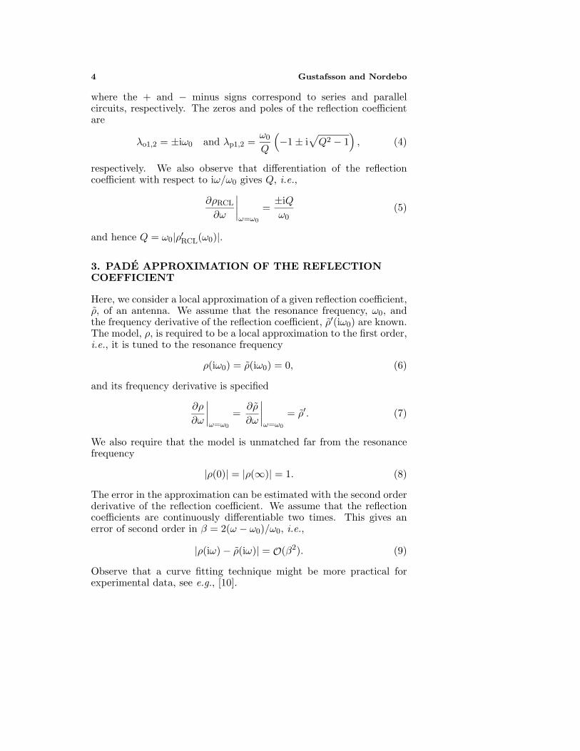
Figure 1. Lumped circuits. a) the series RCL circuit. b) the parallelRCL circuit. c) a lattice network.

there is an extensive literature on the Q factor for antennas, seee.g., [2, 3, 6, 7, 14], only some of the results are given here. TheQ factor of the antenna is defined as the quotient between the powerstored in the reactive field and the radiated power [2, 3], i.e.,

Q =2ω max(WM,WE)

P, (1)

where ω is the angular frequency, WM the stored magnetic energy,WE the stored electric energy, and P the dissipated power. At theresonance frequency, ω0, there are equal amounts of stored electricenergy and stored magnetic energy, i.e., WE = WM.

The Q factor is also fundamentally related to the lumpedresonance circuits [11]. The basic series (parallel) resonance circuitconsists of series (parallel) connected inductor, capacitor, and resistor,see Figure 1ab. With a resonance frequency ω0 and resistance R,we have L = RQ/ω0 and C = 1/(RQω0) and L = R/(Qω0) andC = Q/(Rω0) in the series and parallel cases, respectively. It is easilyseen that the Q factor defined in (1) is consistent with the lumpedresonance circuits [11].

The transmission coefficient of the resonance circuits inFigure 1ab, is

tRCL(s) =1

1 +Q

2

(ω0

s+

s

ω0

) , (2)

where s = σ + iω denote the Laplace parameter. It has one zero atthe origin, s = 0, and one zero at infinity, s = ∞. The correspondingreflection coefficient is

ρRCL(s) =Z(s) −R

Z(s) + R= ± 1 + (s/ω0)2

1 + (s/ω0)2 + 2s/(ω0Q)(3)


where the + and − minus signs correspond to series and parallelcircuits, respectively. The zeros and poles of the reflection coefficientare

λo1,2 = ±iω0 and λp1,2 =ω0

Q

(−1 ± i

√Q2 − 1

), (4)

respectively. We also observe that differentiation of the reflectioncoefficient with respect to iω/ω0 gives Q, i.e.,

∂ρRCL

∂ω

∣∣∣∣ω=ω0

=±iQω0

(5)

and hence Q = ω0|ρ′RCL(ω0)|.

3. PADE APPROXIMATION OF THE REFLECTIONCOEFFICIENT

Here, we consider a local approximation of a given reflection coefficient,ρ, of an antenna. We assume that the resonance frequency, ω0, andthe frequency derivative of the reflection coefficient, ρ′(iω0) are known.The model, ρ, is required to be a local approximation to the first order,i.e., it is tuned to the resonance frequency

ρ(iω0) = ρ(iω0) = 0, (6)

and its frequency derivative is specified

∂ρ

∂ω

∣∣∣∣ω=ω0

=∂ρ

∂ω

∣∣∣∣ω=ω0

= ρ′. (7)

We also require that the model is unmatched far from the resonancefrequency

|ρ(0)| = |ρ(∞)| = 1. (8)

The error in the approximation can be estimated with the second orderderivative of the reflection coefficient. We assume that the reflectioncoefficients are continuously differentiable two times. This gives anerror of second order in β = 2(ω − ω0)/ω0, i.e.,

|ρ(iω) − ρ(iω)| = O(β2). (9)

Observe that a curve fitting technique might be more practical forexperimental data, see e.g., [10].


We start with a Pade approximation of the reflection coefficient.A general Pade approximation of order 2,2 is

ρ(s) = γ1 + a1s + a2s

2

1 + b1s + b2s2(10)

where a1, a2, b1, b2 are real valued constants. As the reflectioncoefficient has an arbitrary phase at resonance, it is necessary toconsider a complex valued coefficient γ. We interpret this as a slowlyvarying function γ(s) where γ(iω) ≈ γ over the considered frequencyinterval. The requirement (8) gives |γ| = 1 and |a2| = |b2|. We alsohave γ(−iω) ≈ γ∗ for any physically realizable model. The resonancefrequency imply a1 = 0 and a2 = ω−2

0 . Differentiation with respect tothe angular frequency gives

γ− 2ω0

1 + b1iω0 − b2ω20

= ρ′ (11)

and hence b2 = ω−20 and b1 = 2/(ω0Qρ), where we have introduced the

Q factor in the resonance approximation as

Qρ = |ρ′(iω0)ω0| (12)

in accordance with (5). We observe the resemblance with the approachin [14] showing that the Q factor of some antennas, Q, can beapproximated with the frequency derivative of the impedance, i.e.,

Q ≈ ω0|Z ′

1|2R

= ω0|ρ′| = Qρ. (13)

The Pade approximation of the reflection coefficient can be written

ρ(s) =−iρ′

|ρ′|1 + (s/ω0)2

1 + (s/ω0)2 + 2s/(ω0Qρ). (14)

The special case with arg ρ′ = π/2 (arg ρ′ = −π/2) gives the classicallumped series (parallel) RCL circuit approximation. Observe that Qρ

is the Q factor of the approximating resonance circuit and not the Qfactor of the original system.

We can interpret the general cases with �ρ′ �= 0 as the result with acascade coupled RCL circuit and a transmission line with characteristicimpedance R. A transmission line with length d rotates the reflectioncoefficient an angle φ = −2dk0 = −2dω0/c0 in the complex plane. Itis also possible to consider a lattice network that rotates the reflection


coefficient [13]. A lattice network with capacitance, C, and inductance,L = R2C, as shown in Figure 1, has reflection coefficient ρL(s) = 0and transmission coefficient

tL(s) =1 − sRC

1 + sRC=

1 − αs/ω0

1 + αs/ω0, (15)

where we have introduced the dimensional free parameter α = ω0RC.The reflection coefficient of the cascaded lattice and RCL circuit is

ρ(s) = t2L(s)ρRCL(s) = ±(

1 − αs/ω0

1 + αs/ω0

)2 1 + (s/ω0)2

1 + (s/ω0)2 + 2s/ω0/Qρ

(16)

where it is seen that the lattice network rotates the reflection coefficientan angle φ = −4 arctan(α). It is easily seen that α = − tan(φ/4) andhence 0 < α < 1 as it is sufficient to consider −π < φ < 0. Thetransmission coefficient of the cascaded system is given by t = tLtRCL.

4. BANDWIDTH AND MATCHING

The reflection coefficient (16) provides a local approximation of thereflection coefficient of the antenna. Assume that the error of thereflection coefficient of the approximate circuit is of size ε, i.e.,

|ρ(iω) − ρ(iω)| ≤ ε (17)

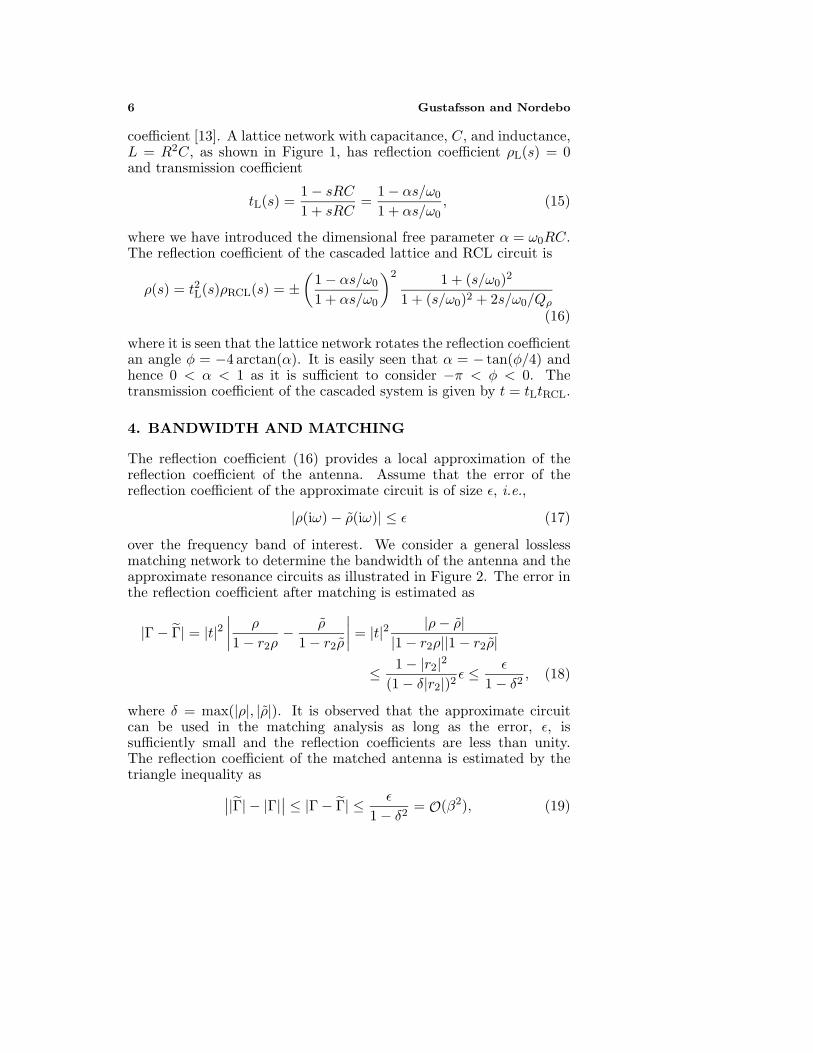
over the frequency band of interest. We consider a general losslessmatching network to determine the bandwidth of the antenna and theapproximate resonance circuits as illustrated in Figure 2. The error inthe reflection coefficient after matching is estimated as

|Γ − Γ| = |t|2∣∣∣∣ ρ

1 − r2ρ− ρ

1 − r2ρ

∣∣∣∣ = |t|2 |ρ− ρ||1 − r2ρ||1 − r2ρ|

≤ 1 − |r2|2(1 − δ|r2|)2

ε ≤ ε

1 − δ2, (18)

where δ = max(|ρ|, |ρ|). It is observed that the approximate circuitcan be used in the matching analysis as long as the error, ε, issufficiently small and the reflection coefficients are less than unity.The reflection coefficient of the matched antenna is estimated by thetriangle inequality as∣∣|Γ| − |Γ|

∣∣ ≤ |Γ − Γ| ≤ ε

1 − δ2= O(β2), (19)


t

r2r1

Z

t

r2r1 ρ˜ ˜

a)

b)

Zρ

Γ

Γmatchingnetwork

matchingnetwork

resonance

antenna

Figure 2. Illustration of the lossless matching networks. Thematching network has the reflection coefficients r1 and r2 andtransmission coefficient t. The same matching network is used in thetwo cases. a) the resonance circuit with reflection coefficient ρ gives Γ.b) the antenna with reflection coefficient ρ gives Γ.

where we used (9).The Bode-Fano theory is used to get fundamental limitations

on the matching network [4, 12]. The Bode-Fano theory usesTaylor expansions of the reflection coefficient around the zeros ofthe transmission coefficient to get a set of integral relations for thereflection coefficient. We start with the lumped RCL circuit. Thetransmission coefficient (2) of the RCL circuit has a single zero at theorigin and a single zero at infinity. The Bode-Fano theory gives theintegral relations

2π

∫ ∞

0

1ω2

ln1

|Γ(iω)|dω =∑

i

λ−1oi − λ−1

pi − 2λ−1ri =

2ω0Q

− 2∑

i

λ−1ri

(20)

and

2π

∫ ∞

0ln

1|Γ(iω)|dω =

∑i

λoi − λpi − 2λri = 2ω0

Q− 2

∑i

λri (21)

by a Taylor expansion around s = 0 and s = ∞, respectively. Here,λoi, λpi, and λri denote the zeros (4) of ρRCL, the poles (4) of ρRCL, andarbitrary complex valued numbers with positive real part, respectively.We assume that the matching is symmetric around the resonancefrequency, i.e., the frequency range ω0 − ∆ω/2 ≤ ω ≤ ω0 + ∆ω/2


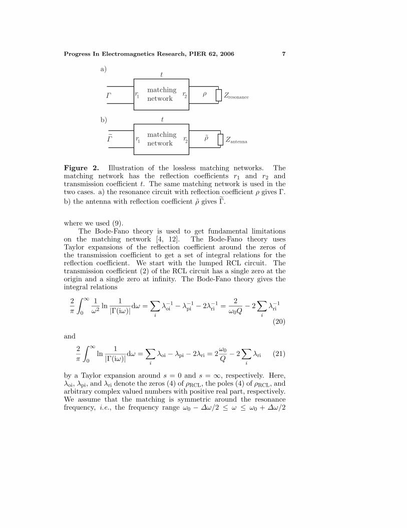
Figure 3. Illustration of the Bode-Fano limits. The model givesthe threshold Γ0. The threshold level of the corresponding antennais estimated with (19). The dashed curve illustrates an unattainablereflection coefficient.

is considered. The relative bandwidth, B, is given by B = ∆ω/ω0. Set

K = inf| ωω0

−1|≤B2

2π

ln1

|Γ(iω)| =2π

ln1

sup| ωω0

−1|≤B2|Γ(iω)| (22)

to simplify the notation [4].The integrals in (20) and (21) are estimated from below giving

B

1 −B2/4K ≤ 2

Q− 2

∑i

ω0

λriand BK ≤ 2

Q− 2

∑i

λri

ω0, (23)

where the coefficients λri have a positive real-valued part. Bothinequalities can be satisfied with a complex conjugated par, λr1 = λ∗

r2.This reduces the inequalities to

K ≤ 2BQ

(1 − B2

4

). (24)

Hence, the reflection coefficient is bounded as

sup |Γ(iω)| ≥ Γ0 = e−π

QB(1−B2/4) = e−

πQB + O(B/Q) (25)


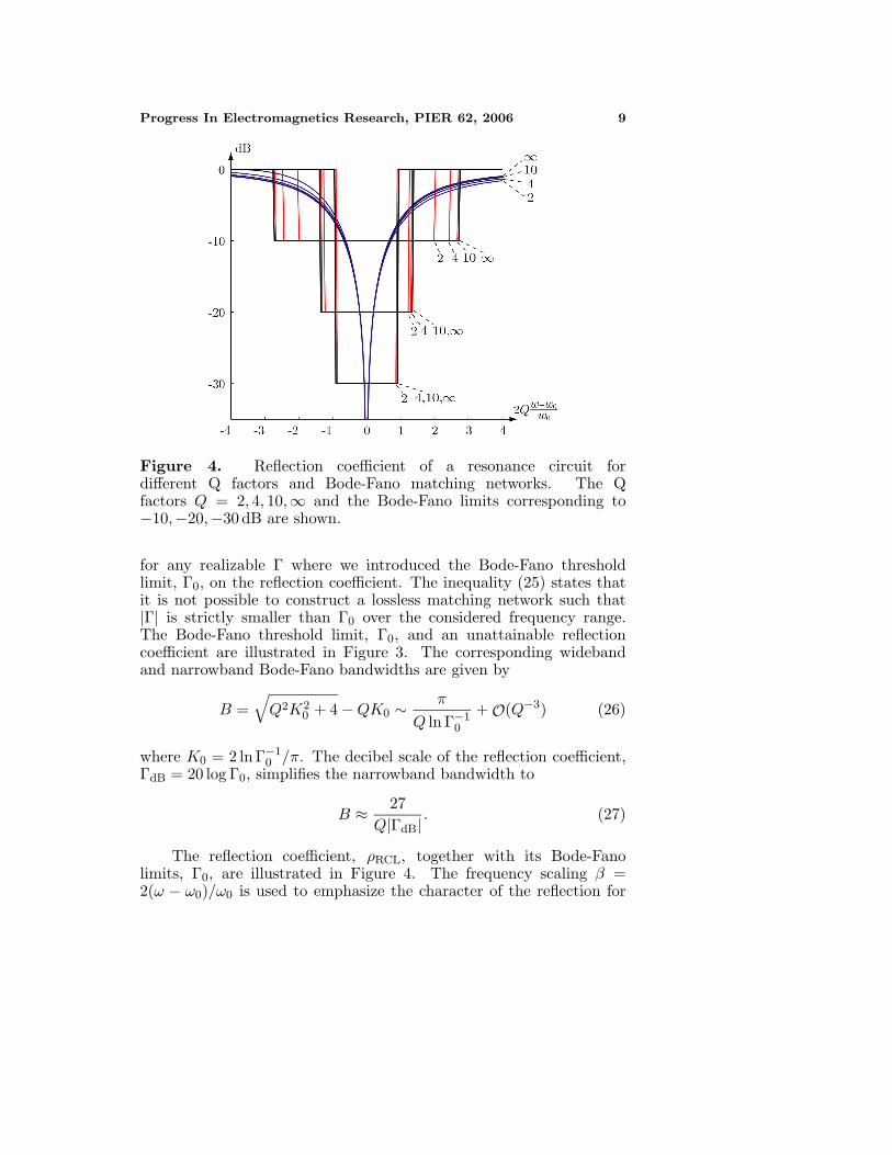
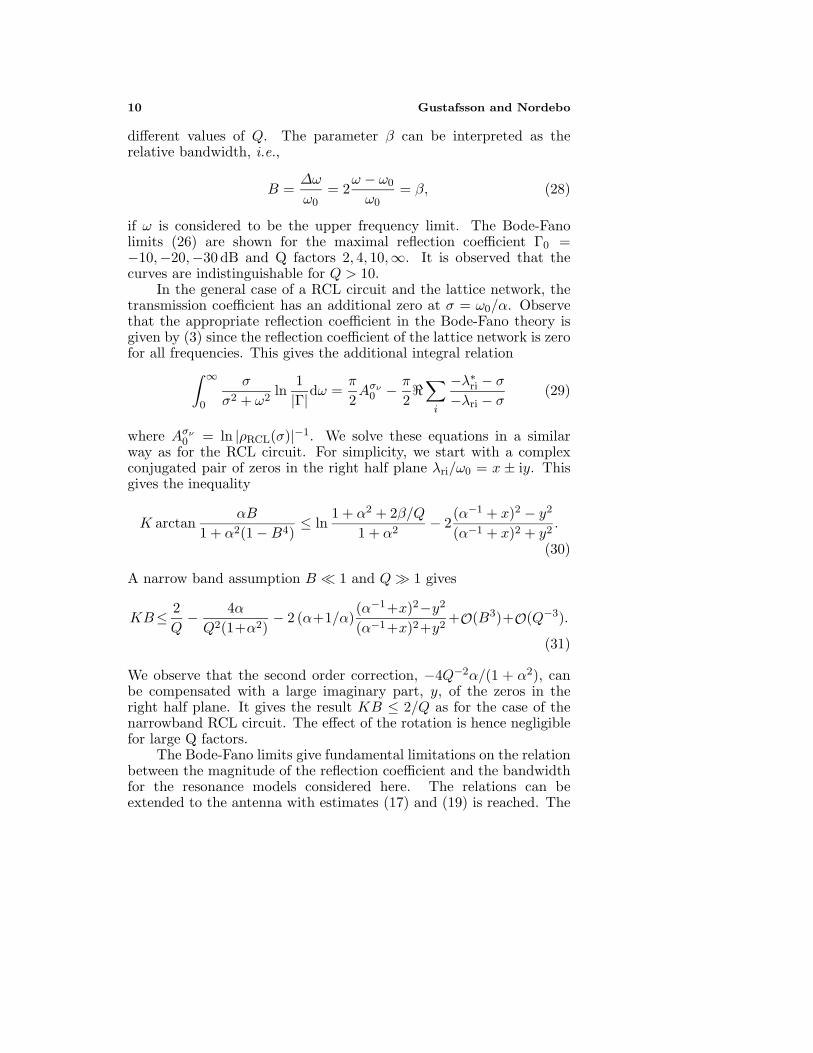
Figure 4. Reflection coefficient of a resonance circuit fordifferent Q factors and Bode-Fano matching networks. The Qfactors Q = 2, 4, 10,∞ and the Bode-Fano limits corresponding to−10,−20,−30 dB are shown.

for any realizable Γ where we introduced the Bode-Fano thresholdlimit, Γ0, on the reflection coefficient. The inequality (25) states thatit is not possible to construct a lossless matching network such that|Γ| is strictly smaller than Γ0 over the considered frequency range.The Bode-Fano threshold limit, Γ0, and an unattainable reflectioncoefficient are illustrated in Figure 3. The corresponding widebandand narrowband Bode-Fano bandwidths are given by

B =√

Q2K20 + 4 −QK0 ∼ π

Q ln Γ−10

+ O(Q−3) (26)

where K0 = 2 ln Γ−10 /π. The decibel scale of the reflection coefficient,

ΓdB = 20 log Γ0, simplifies the narrowband bandwidth to

B ≈ 27Q|ΓdB|

. (27)

The reflection coefficient, ρRCL, together with its Bode-Fanolimits, Γ0, are illustrated in Figure 4. The frequency scaling β =2(ω − ω0)/ω0 is used to emphasize the character of the reflection for


different values of Q. The parameter β can be interpreted as therelative bandwidth, i.e.,

B =∆ω

ω0= 2

ω − ω0

ω0= β, (28)

if ω is considered to be the upper frequency limit. The Bode-Fanolimits (26) are shown for the maximal reflection coefficient Γ0 =−10,−20,−30 dB and Q factors 2, 4, 10,∞. It is observed that thecurves are indistinguishable for Q > 10.

In the general case of a RCL circuit and the lattice network, thetransmission coefficient has an additional zero at σ = ω0/α. Observethat the appropriate reflection coefficient in the Bode-Fano theory isgiven by (3) since the reflection coefficient of the lattice network is zerofor all frequencies. This gives the additional integral relation∫ ∞

0

σ

σ2 + ω2ln

1|Γ|dω =

π

2Aσν

0 − π

2�

∑i

−λ∗ri − σ

−λri − σ(29)

where Aσν0 = ln |ρRCL(σ)|−1. We solve these equations in a similar

way as for the RCL circuit. For simplicity, we start with a complexconjugated pair of zeros in the right half plane λri/ω0 = x ± iy. Thisgives the inequality

K arctanαB

1 + α2(1 −B4)≤ ln

1 + α2 + 2β/Q1 + α2

− 2(α−1 + x)2 − y2

(α−1 + x)2 + y2.

(30)

A narrow band assumption B � 1 and Q 1 gives

KB≤ 2Q

− 4αQ2(1+α2)

− 2 (α+1/α)(α−1+x)2−y2

(α−1+x)2+y2+O(B3)+O(Q−3).

(31)

We observe that the second order correction, −4Q−2α/(1 + α2), canbe compensated with a large imaginary part, y, of the zeros in theright half plane. It gives the result KB ≤ 2/Q as for the case of thenarrowband RCL circuit. The effect of the rotation is hence negligiblefor large Q factors.

The Bode-Fano limits give fundamental limitations on the relationbetween the magnitude of the reflection coefficient and the bandwidthfor the resonance models considered here. The relations can beextended to the antenna with estimates (17) and (19) is reached. The


reflection coefficient of the antenna after matching is estimated by (19)as

sup |Γ| = Γ0 ≥ Γ0 −ε

1 − δ2= e−

πQB + O(ε). (32)

where sup |Γ| = Γ0 = e−π/(QρB). Invert to get an estimate of thebandwidth

B ≤ π

Qρ ln(Γ0 + ε/(1 − δ2))−1≈ π

Qρ ln Γ−10

(1 +

ε

Γ0 ln Γ−10 (1 − δ2)

)=

π

Qρ ln Γ−10

+ O(ε) =π

Qρ ln Γ−10

+ O(B2), (33)

where we used the estimate (19). Hence, the bandwidth of the antennacan be estimated by the Q factor, Qρ = ω0|ρ′|, of the approximatingresonance model as long as the bandwidth is sufficiently narrow giving

B ∼ π

Qρ ln Γ−10

, for B � 1. (34)

5. APPROXIMATION OF SPHERICAL VECTOR WAVES

An arbitrary electromagnetic field can be expanded in spherical vectorwaves [1, 8, 9]

E(r) =∞∑l=1

l∑m=−l

2∑τ=1

aτmlvτml(kr) + fτmluτml(kr) (35)

H(r) =iη0

∞∑l=1

l∑m=−l

2∑τ=1

aτmlvτml(kr) + fτmluτml(kr) (36)

The terms labeled by τ = 1, l, and m identify magnetic 2l-poles andthe terms labeled by τ = 2, l, and m identify electric 2l-poles. Theoutgoing spherical vector waves u are given by

u1ml(kr) = h(2)l (kr)A1ml(r) (37)

u2ml(kr) =1k∇×

(h

(2)l (kr)A1ml(r)

)(38)

where h(2)l denotes the spherical Hankel function and A denote the

spherical vector harmonics. There are several common definitions of


the spherical vector harmonics [1, 8, 9]. For τ = 1, 2, we use

A1ml(r) =1√

l(l + 1)∇× (r Ym

l (r)) (39)

A2ml(r) = r × A1ml(r), (40)

where Yml denotes the spherical harmonics [1, 8, 9].

The impedance of a TM mode normalized with the intrinsicimpedance, η0, is (ξ = ka = ωa/c0)

Z = R + iX = i(ξ h

(2)l (ξ))′

ξ h(2)l (ξ)

=1

|ξ h(2)l |2

+ i�(ξ h(2)l )′

ξ h(2)l

(41)

where we used the Wronskian h(2)l h

(2)l

′∗ − h(2)l

∗ h(2)l

′ = 2iξ−2. Theseries expansions of the Hankel functions [9] gives the expansions

R(ξ) ∼ ξ2l l!2l

(2l)!and X ∼ − l

ξ(42)

for small ξ. Tune the impedance with a series inductor, i.e., ω0L =−X. This gives the impedance Z1 = Z + iωL. Differentiate theimpedance with respect to the angular frequency ω

Z ′1 = −2R

a

c0�(ξ h

(2)l )′

ξ h(2)l

+ia

c0

n(n+1)ξ2

−1−�(

h(2)l

′

h(2)l

+1ξ

)2

+c0aL

= −2αRX + iα

(n(n + 1)

ξ2− 1 + R2 −X2 − X

ξ

)(43)

The frequency derivative of reflection coefficient, ρ = (Z1−R)/(Z1+R),is given by

ω∂ρ

∂ω= ωρ′ = ω

Z ′1

2R= −kaX +

ika2R

(n(n + 1)k2a2

− X

ka−X2 − 1 + R2

)(44)

The derivatives (44) is used to get resonance models of the TEand TM reflection coefficients, Qρ = ω|ρ′(ω)|. The TM (TE) case givesseries (parallel) circuits combined with lattice networks. In Figure 5a,the reflection coefficient, ρ, together with their resonance models (16)are depicted for spheres with radius k0a = 0.4 and k0a = 0.65. TheTM and TE cases are shown for l = 1 and l = 2, respectively. The


b)a)

518

5

18

AntennaResonance

182, 1859

182, 1859TEm2

TMm1

TEm2

TMm1

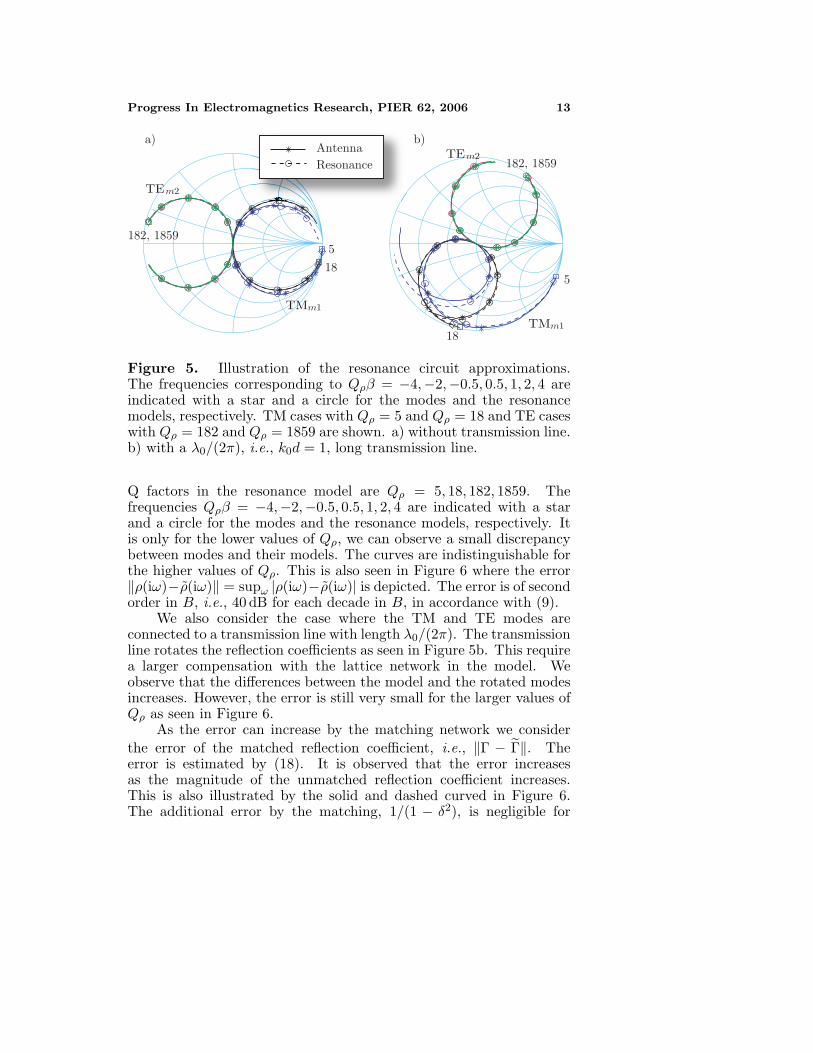
Figure 5. Illustration of the resonance circuit approximations.The frequencies corresponding to Qρβ = −4,−2,−0.5, 0.5, 1, 2, 4 areindicated with a star and a circle for the modes and the resonancemodels, respectively. TM cases with Qρ = 5 and Qρ = 18 and TE caseswith Qρ = 182 and Qρ = 1859 are shown. a) without transmission line.b) with a λ0/(2π), i.e., k0d = 1, long transmission line.

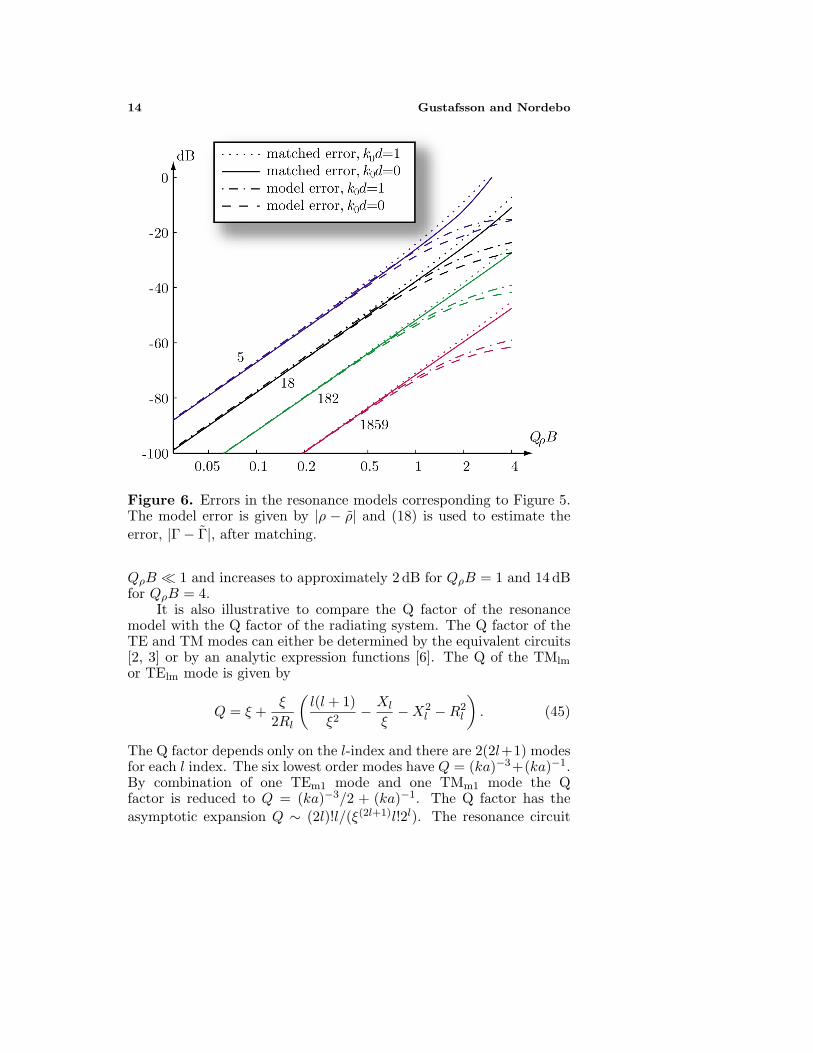
Q factors in the resonance model are Qρ = 5, 18, 182, 1859. Thefrequencies Qρβ = −4,−2,−0.5, 0.5, 1, 2, 4 are indicated with a starand a circle for the modes and the resonance models, respectively. Itis only for the lower values of Qρ, we can observe a small discrepancybetween modes and their models. The curves are indistinguishable forthe higher values of Qρ. This is also seen in Figure 6 where the error‖ρ(iω)−ρ(iω)‖ = supω |ρ(iω)−ρ(iω)| is depicted. The error is of secondorder in B, i.e., 40 dB for each decade in B, in accordance with (9).

We also consider the case where the TM and TE modes areconnected to a transmission line with length λ0/(2π). The transmissionline rotates the reflection coefficients as seen in Figure 5b. This requirea larger compensation with the lattice network in the model. Weobserve that the differences between the model and the rotated modesincreases. However, the error is still very small for the larger values ofQρ as seen in Figure 6.

As the error can increase by the matching network we considerthe error of the matched reflection coefficient, i.e., ‖Γ − Γ‖. Theerror is estimated by (18). It is observed that the error increasesas the magnitude of the unmatched reflection coefficient increases.This is also illustrated by the solid and dashed curved in Figure 6.The additional error by the matching, 1/(1 − δ2), is negligible for


Figure 6. Errors in the resonance models corresponding to Figure 5.The model error is given by |ρ − ρ| and (18) is used to estimate theerror, |Γ − Γ|, after matching.

QρB � 1 and increases to approximately 2 dB for QρB = 1 and 14 dBfor QρB = 4.

It is also illustrative to compare the Q factor of the resonancemodel with the Q factor of the radiating system. The Q factor of theTE and TM modes can either be determined by the equivalent circuits[2, 3] or by an analytic expression functions [6]. The Q of the TMlm

or TElm mode is given by

Q = ξ +ξ

2Rl

(l(l + 1)

ξ2− Xl

ξ−X2

l −R2l

). (45)

The Q factor depends only on the l-index and there are 2(2l+1) modesfor each l index. The six lowest order modes have Q = (ka)−3+(ka)−1.By combination of one TEm1 mode and one TMm1 mode the Qfactor is reduced to Q = (ka)−3/2 + (ka)−1. The Q factor has theasymptotic expansion Q ∼ (2l)!l/(ξ(2l+1)l!2l). The resonance circuit


1 10 100

10-4

10 -3

10 -2

10 -1

100

relative error

Q

narrowband RCLwideband RCL

B–BQ|B

|

B–B |B

| Qρ

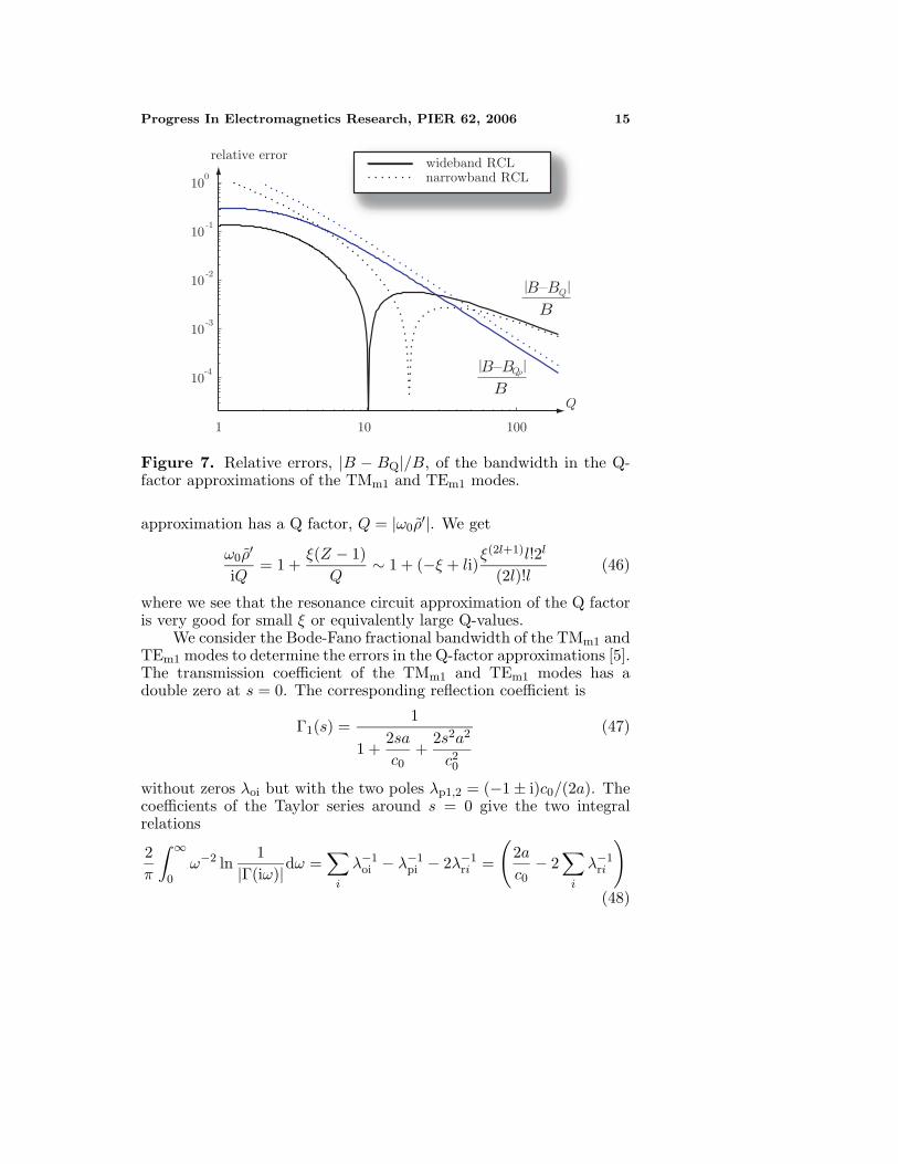
Figure 7. Relative errors, |B − BQ|/B, of the bandwidth in the Q-factor approximations of the TMm1 and TEm1 modes.

approximation has a Q factor, Q = |ω0ρ′|. We get

ω0ρ′

iQ= 1 +

ξ(Z − 1)Q

∼ 1 + (−ξ + li)ξ(2l+1)l!2l

(2l)!l(46)

where we see that the resonance circuit approximation of the Q factoris very good for small ξ or equivalently large Q-values.

We consider the Bode-Fano fractional bandwidth of the TMm1 andTEm1 modes to determine the errors in the Q-factor approximations [5].The transmission coefficient of the TMm1 and TEm1 modes has adouble zero at s = 0. The corresponding reflection coefficient is

Γ1(s) =1

1 +2sac0

+2s2a2

c20

(47)

without zeros λoi but with the two poles λp1,2 = (−1 ± i)c0/(2a). Thecoefficients of the Taylor series around s = 0 give the two integralrelations

2π

∫ ∞

0ω−2 ln

1|Γ(iω)|dω =

∑i

λ−1oi − λ−1

pi − 2λ−1ri =

(2ac0

− 2∑

i

λ−1ri

)(48)


and

2π

∫ ∞

0ω−4 ln

1|Γ(iω)|dω =

−13

∑i

1λ3

oi

− 1λ3

pi

− 2λ3

ri

=

(4a3

3c30+

23

∑i

λ−3ri

),

(49)

where the coefficients λri have a positive real-valued part. Assuming abandwidth and K as in (22) gives

KB

1 −B2/4≤ 2k0a− 2

∑i

ω0

λr(50)

and

KB + B3/12(1 −B2/4)3

≤ 4(k0a)3

3+

23

∑i

ω30

λ3r

(51)

where k0 = ω0/c0. It is noted that it is enough to consider onecoefficient λr or a complex conjugated pair. These equations can besolved numerically with respect to B and λr.

The fractional bandwidth, B, given by (50) and (51) iscompared with the fractional bandwidth, BQ, determined by theresonance approximation (26) to determine the error in the resonanceapproximation. We consider the Q factors determined by thestored and radiated fields (1), i.e., (45), and by the resonanceapproximation (12), i.e., (44). The relative error |B − BQ|/B isdepicted in Figure 7 for the threshold reflection coefficient Γ0 = 1/3. Itis observed that the errors are small for large Q factors and that theyapproach 0 as Q → ∞ as known from the asymptotic expansions. Wealso observe that the narrowband approximation in (26) is good forlarge Q factors. The error of the resonance approximation, Qρ, decaysfaster than the error in the Q-approximation as Q increases. This is inaccordance with the construction of the resonance approximation as alocal approximation of the reflection coefficient.

6. Q FACTOR OF GENERAL ANTENNAS

There have been several attempts to express the Q factor of a generalantenna in the impedance of the antenna, see [14] and references therein. Common versions are

Q ≈ ω0

2R(ω0)|X ′(ω0)| (52)


simpleantenna

microwavenetwork

shieldedpowersupply

S1S2

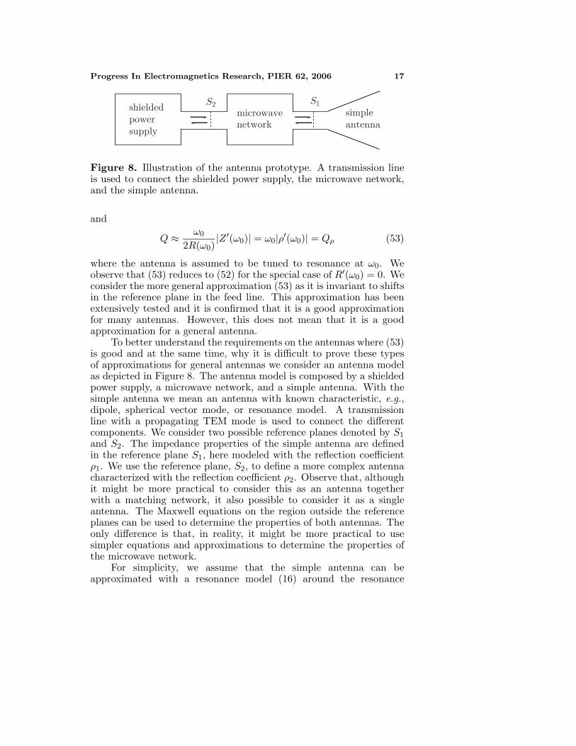
Figure 8. Illustration of the antenna prototype. A transmission lineis used to connect the shielded power supply, the microwave network,and the simple antenna.

and

Q ≈ ω0

2R(ω0)|Z ′(ω0)| = ω0|ρ′(ω0)| = Qρ (53)

where the antenna is assumed to be tuned to resonance at ω0. Weobserve that (53) reduces to (52) for the special case of R′(ω0) = 0. Weconsider the more general approximation (53) as it is invariant to shiftsin the reference plane in the feed line. This approximation has beenextensively tested and it is confirmed that it is a good approximationfor many antennas. However, this does not mean that it is a goodapproximation for a general antenna.

To better understand the requirements on the antennas where (53)is good and at the same time, why it is difficult to prove these typesof approximations for general antennas we consider an antenna modelas depicted in Figure 8. The antenna model is composed by a shieldedpower supply, a microwave network, and a simple antenna. With thesimple antenna we mean an antenna with known characteristic, e.g.,dipole, spherical vector mode, or resonance model. A transmissionline with a propagating TEM mode is used to connect the differentcomponents. We consider two possible reference planes denoted by S1

and S2. The impedance properties of the simple antenna are definedin the reference plane S1, here modeled with the reflection coefficientρ1. We use the reference plane, S2, to define a more complex antennacharacterized with the reflection coefficient ρ2. Observe that, althoughit might be more practical to consider this as an antenna togetherwith a matching network, it also possible to consider it as a singleantenna. The Maxwell equations on the region outside the referenceplanes can be used to determine the properties of both antennas. Theonly difference is that, in reality, it might be more practical to usesimpler equations and approximations to determine the properties ofthe microwave network.

For simplicity, we assume that the simple antenna can beapproximated with a resonance model (16) around the resonance


R

Qw0

R

Qw0

1

w0

Qw0

QRR

R

1

1

2

2ρ

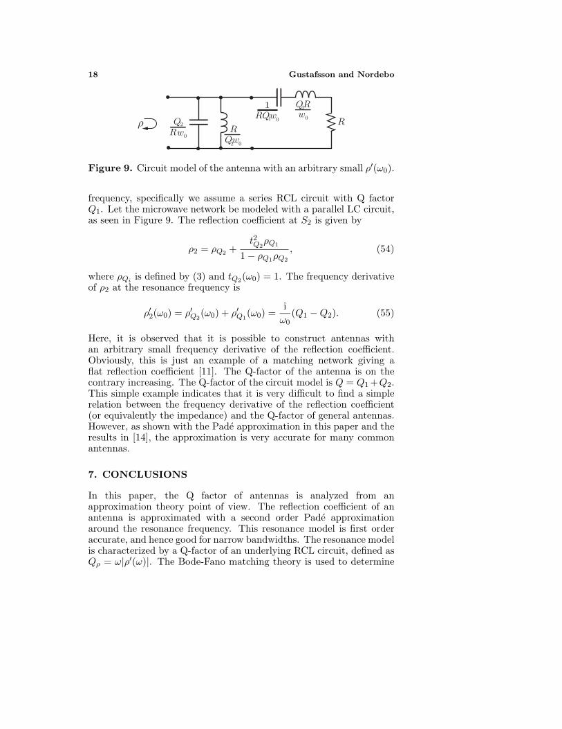
Figure 9. Circuit model of the antenna with an arbitrary small ρ′(ω0).

frequency, specifically we assume a series RCL circuit with Q factorQ1. Let the microwave network be modeled with a parallel LC circuit,as seen in Figure 9. The reflection coefficient at S2 is given by

ρ2 = ρQ2 +t2Q2

ρQ1

1 − ρQ1ρQ2

, (54)

where ρQi is defined by (3) and tQ2(ω0) = 1. The frequency derivativeof ρ2 at the resonance frequency is

ρ′2(ω0) = ρ′Q2(ω0) + ρ′Q1

(ω0) =iω0

(Q1 −Q2). (55)

Here, it is observed that it is possible to construct antennas withan arbitrary small frequency derivative of the reflection coefficient.Obviously, this is just an example of a matching network giving aflat reflection coefficient [11]. The Q-factor of the antenna is on thecontrary increasing. The Q-factor of the circuit model is Q = Q1 +Q2.This simple example indicates that it is very difficult to find a simplerelation between the frequency derivative of the reflection coefficient(or equivalently the impedance) and the Q-factor of general antennas.However, as shown with the Pade approximation in this paper and theresults in [14], the approximation is very accurate for many commonantennas.

7. CONCLUSIONS

In this paper, the Q factor of antennas is analyzed from anapproximation theory point of view. The reflection coefficient of anantenna is approximated with a second order Pade approximationaround the resonance frequency. This resonance model is first orderaccurate, and hence good for narrow bandwidths. The resonance modelis characterized by a Q-factor of an underlying RCL circuit, defined asQρ = ω|ρ′(ω)|. The Bode-Fano matching theory is used to determine


the bandwidth of the approximate model. Moreover, it is shown thatthe original antenna has the same bandwidth for sufficiently narrowbandwidths.

Even if the Q-factor, defined by the stored and radiated energies,of the antenna system is not used in the analysis, there is a closeresemblance between the Q-factor derived from the differentiatedreflection coefficient, Qρ, and the classical Q-factor, Q. It is shownthat Q ≈ Qρ for each spherical vector mode if Q is sufficiently large.This is also seen for many antennas from the approximation of theQ-factor Q ≈ ω|Z ′|/(2R) = Qρ considered in [14]. However, a simpleexample is used to illustrate that there is not a simple relation betweenQ and Qρ for every antenna.

ACKNOWLEDGMENT

The financial support by the Swedish research council is gratefullyacknowledged.

REFERENCES

1. Arfken, G., Mathematical Methods for Physicists, third ed.,Academic Press, Orlando, 1985.

2. Chu, L. J., “Physical limitations of omni-directional antennas,”Appl. Phys., Vol. 19, 1163–1175, 1948.

3. Collin, R. E. and S. Rothschild, “Evaluation of antenna Q,” IEEETrans. Antennas Propagat., Vol. 12, 23–27, Jan. 1964.

4. Fano, R. M., “Theoretical limitations on the broadband matchingof arbitrary impedances,” Journal of the Franklin Institute,Vol. 249, Nos. 1,2, 57–83 and 139–154, 1950.

5. Gustafsson, M. and S. Nordebo, “On the spectral efficiency of asphere,” Tech. Rep. LUTEDX/(TEAT-7127)/1–24/(2004), LundInstitute of Technology, Department of Electroscience, P.O. Box118, S-211 00 Lund, Sweden, 2004. http://www.es.lth.se/teorel.

6. Hansen, R. C., “Fundamental limitations in antennas,” Proc.IEEE, Vol. 69, No. 2, 170–182, 1981.

7. Harrington, R. F., Time Harmonic Electromagnetic Fields,McGraw-Hill, New York, 1961.

8. Jackson, J. D., Classical Electrodynamics, second ed., John Wiley& Sons, New York, 1975.

9. Newton, R. G., Scattering Theory of Waves and Particles, seconded., Dover Publications, New York, 2002.


10. Petersan, P. J. and S. M. Anlage, “Measurement of resonantfrequency and quality factor of microwave resonators: Comparisonof methods,” Appl. Phys., Vol. 84, No. 6, 3392–3402, Sept. 1998.

11. Pozar, D. M., Microwave Engineering, John Wiley & Sons, NewYork, 1998.

12. Vassiliadis, A. and R. L. Tanner, “Evaluating the impedancebroadbanding potential of antennas,” IRE Trans. on Antennasand Propagation, Vol. 6, No. 3, 226–231, July 1958.

13. Willson, A. N. and H. J. Orchard, “Insights into digital filltersmade as the sum of two allpass functions,” IEEE Trans. onCircuits and Systems I: Fundamental theory and applications,Vol. 42, No. 3, 129–137, 1995.

14. Yaghjian, A. D. and S. R. Best, “Impedance, bandwidth, and Qof antennas,” IEEE Trans. Antennas Propagat., Vol. 53, No. 4,1298–1324, 2005.

BANDWIDTH,QFACTOR,ANDRESONANCE ... transmission coeﬃcient of the resonance circuits in...

Documents

Transcript of BANDWIDTH,QFACTOR,ANDRESONANCE ... transmission coeﬃcient of the resonance circuits in...