
arXiv:hep-th/0110067v2 13 Jan 2006
132
arXiv:hep-th/0110067v2 13 Jan 2006 Heterotic, Open and Unoriented String Theories from Topological Membrane Pedro Castelo Caetano Ferreira Department of Physics Keble College University of Oxford Thesis submitted for the degree of Doctor of Philosophy in the University of Oxford Supervisor: Ian I. Kogan 5th October 2001, Michaelmas term
Transcript of arXiv:hep-th/0110067v2 13 Jan 2006

arX
iv:h
ep-t
h/01
1006
7v2
13
Jan
2006
Heterotic, Open and Unoriented String Theories
from Topological Membrane
Pedro Castelo Caetano Ferreira
Department of Physics
Keble College
University of Oxford
Thesis submitted for the degree of Doctor of Philosophy
in the University of Oxford
Supervisor: Ian I. Kogan
5th October 2001, Michaelmas term


Heterotic, Open and Unoriented String Theories
from Topological Membrane
Pedro Castelo Caetano Ferreira
Department of Physics
Keble College
University of Oxford
Abstract
In this work I consider several topics in the Topological Membrane (TM) approach
to string theory. In TM the string worldsheets emerge as boundary theories of
the 3D membrane with topology Σ × [0, 1]. The string dynamics is generated
in this way from the bulk physics, namely from the 3D Topologically Massive
Gauge Theory (TMGT) and Topologically Massive Gravity (TMG).
Both (equivalent) path integral and canonical methods of quantizing TMGT are
considered. When this theory is defined on a manifold with two disconnected
boundaries there are induced chiral Conformal Field Theories (CFT’s) on the
boundaries which can be interpreted as the left and right sectors of closed strings.
A detailed study of the charge spectrum of 3D Abelian TMGT is given. It is
shown that Narain constraints on toroidal compactification (integer, even, self-
dual momentum lattice) have a natural interpretation in purely three dimensional
terms. This is an important result which is necessary to construct toroidal com-
pactification and the heterotic string from TM(GT). The block structure of c = 1
Rational Conformal Field Theory (RCFT) from the point of view of three dimen-
sional field theory is also derived.
Open and unoriented strings in TM(GT) theory are also studied through orbifolds
of the bulk 3D space. This is achieved by gauging discrete symmetries of the
theory. Open and unoriented strings can be obtained from all possible realizations
of C, P and T symmetries. The important role of C symmetry to distinguish
between Dirichlet and Neumann boundary conditions is discussed in detail.
Future directions of research in this field are also suggested and discussed.
Thesis submitted for the degree of Doctor of Philosophy
in the University of Oxford
5th October 2001, Michaelmas term


Acknowledgments
Firstly I would like to thank Ian Kogan for his guidance in physics and his personal
support over the last four years.
I would like to thank my collaborator Bayram Tekin.
Also I thank Alex Kovner and Andre Lukas for many discussions, suggestions
and their patience.
Thanks also to Martin Schvellinger and Arshad Momen for several discussions.
I thank my examiners John Weather and Richard Szabo as well for their sugges-
tions and comments.
Further I would like to thank my colleagues Mario Santos, Nuno Reis, Florian
Merz, Emiliano Papa, Adrian Campbell Smith, Dave Skinner, Alex Nichols,
Gloria Luzon, Jose Natario, Francesco Mancini, Fermin Viniegra, Sanjay and
specially to Guilherme Milhano and Joao Correia for they company and for sev-
eral discussions.
Thanks to my friends in Oxford, Rob Wallis, Jose Fernandez-Calvo, Charlie
Crichton, Mike Hall, Rebecca Smith, Enda Leaney, Margaret Jackson, Bob Cowan,
James Beresford, Pierre Courtois, Andre Gouveia, Ana Lopes, Patricia Castro,
Yasser Omar, Ruy and Lory Ribeiro for their friendship and specially to Luis
Gomes for his ability for taking me out of troubles.
And finally thanks to my friends faraway Ricardo Alves, Paulo Aurelio Azevedo
Moniz, Silvia Ribeiro, Tiago Perdigao, Jorge Maria and Joao Jorge. Also to C.
for showing me that flowers grow in the desert.
Thanks to my family, Antonio, Irene, Frederico, Rodrigo and Zara for their help
and support over the last four troubled years and specially to Beatriz for always
finding good use for my equations: tearing them apart. Also to her mother,
Maria for the year we have been together in Oxford.
I acknowledge Keble College and the Theoretical Physics Group for receiving me
and for the travel grants, in particular to Janet Betts and Gill Dancey for their
efficiency,
This thesis was supported by PRAXIS XXI/BD/11461/97 grant from FCT (Por-
tugal).


to Beatriz


Als das Kind Kind war, wußte es nicht, daß es Kind war,
alles war ihm beseelt, und alle Seelen waren eins...
Als das Kind Kind war,
war das die Zeit der folgenden Fragen:
Warum bin ich Ich, und warum nicht Du?
Warum bin ich hier und warum nicht dort?
Wann begann die Zeit und wo endet der Raum?
Ist das Leben unter der Sonne nicht bloß ein Traum?
in ”Der Himmel Uber Berlin” (1986) by Wim Wenders


CONTENTS
1. Introduction . . . . . . . . . . . . . . . . . . . . . . . . . . . . . . . . . 1
1.1 3D Chern-Simons Theories . . . . . . . . . . . . . . . . . . . . . . 2
1.2 TMGT - Topologically Massive Gauge Theory . . . . . . . . . . . 4
1.3 Topological Membrane Approach to String Theory . . . . . . . . . 6
1.4 TMG - Topologically Massive Gravity . . . . . . . . . . . . . . . . 8
1.5 Supersymmetry . . . . . . . . . . . . . . . . . . . . . . . . . . . . 12
2. Quantization of TMGT . . . . . . . . . . . . . . . . . . . . . . . . . . . 15
2.1 Path Integral Formalism . . . . . . . . . . . . . . . . . . . . . . . 15
2.2 Canonical Formalism . . . . . . . . . . . . . . . . . . . . . . . . . 25
2.2.1 Wave Function as Boundary Conditions . . . . . . . . . . 27
2.2.2 Conformal Blocks and the CFT Partition Function . . . . 30
3. Toroidal Compactification Spectrum and the Heterotic String . . . . . 35
3.1 Introduction . . . . . . . . . . . . . . . . . . . . . . . . . . . . . . 36
3.1.1 Several U(1)’s and Mass shell condition . . . . . . . . . . . 36
3.1.2 RCFT’s and Fusion Rules . . . . . . . . . . . . . . . . . . 38
3.2 Propagation in the bulk . . . . . . . . . . . . . . . . . . . . . . . 40
3.3 Boundary conditions . . . . . . . . . . . . . . . . . . . . . . . . . 53
3.4 RCFT’s and Fusion Rules . . . . . . . . . . . . . . . . . . . . . . 56
3.5 Lattices and The Heterotic String . . . . . . . . . . . . . . . . . 60
4. Open and Unoriented Strings . . . . . . . . . . . . . . . . . . . . . . . 65
X Contents
4.1 Riemann Surfaces:
from Closed Oriented to Open and Unoriented . . . . . . . . . . . 69
4.1.1 The Projective Plane and the Disk obtained from the Sphere 69
4.1.2 The annulus, Mobius strip and Klein bottle from the Torus 72
4.2 Conformal Field Theory -
Correlation Functions and Boundary Conditions on the Disk . . . 76
4.2.1 Dirichlet Boundary Conditions . . . . . . . . . . . . . . . . 77
4.2.2 Neumann Boundary Conditions . . . . . . . . . . . . . . . 78
4.3 TM(GT) . . . . . . . . . . . . . . . . . . . . . . . . . . . . . . . . 80
4.3.1 Horava Approach to Open World-Sheets . . . . . . . . . . 81
4.3.2 Discrete Symmetries and Orbifolds of TM(GT) . . . . . . 84
4.3.3 Tree Level Amplitudes for
Open and Closed Unoriented Strings . . . . . . . . . . . . 87
4.3.4 One Loop Amplitudes for
Open and Closed Unoriented Strings . . . . . . . . . . . . 96
4.3.5 Note on Modular Invariance and the Relative Modular Group100
4.3.6 Neumann and Dirichlet World-Sheet Boundary Conditions,
Monopole Processes and Charge Conjugation . . . . . . . 104
4.3.7 T-Duality and Several U(1)’s . . . . . . . . . . . . . . . . 106
5. Final Remarks . . . . . . . . . . . . . . . . . . . . . . . . . . . . . . . 109

1. INTRODUCTION
This chapter gives an historical overview of 3D Chern-Simons theory as well as
a short review of the Topological Membrane (TM) approach to string theory.
Not many details are given, only a general overview of past work on the subject.
Some fundamental concepts will be introduced and a description at the level of
the action, justifying the several terms that constitute the full action of TM.
In the remaining of this work only Abelian Topological Massive Gauge Theories
(TMGT) will be addressed in detail.
In Chapter 2 the quantization of TMGT is addressed, both from a path integral
and canonical perspective, and some fundamental issues studied and introduced.
In Chapter 3 the correct toroidal compactification spectrum of bosonic closed
string theories and the heterotic string will be built purely from 3D TM(GT)
physics. The Narain lattice spectrum conditions (Lorentzian even, integer, self
dual lattice) will also be derived. The fusion rules will as well be rederived
from the point of view of the bulk theory. A Heterotic string theory background
encoding the E8 × E8 group will be rederived in the light of these results.
In Chapter 4, open and unoriented string theories are built by orbifolding TM(GT)
and gauging the 3D QFT symmetries PT and PCT . A preliminary discussion
on modular invariance and T-duality is carried out.
Finally Chapter 5 summarizes the accomplishments of this thesis and further
directions of research in these topics are suggested.

2 1. Introduction
1.1 3D Chern-Simons Theories
In mathematical terms the Chern-Simons (CS) term [1] is a topological invariant.
It comes from the Chern class of 4D manifolds. The introduction in physics of
this term in 3D was originally suggested by Schwarz [2] and Singer in unpublished
work on its Abelian version
SCS,a[A] = k
∫
M
d3xA ∧ F (1.1)
where A is some gauge connection field on a 3D manifoldM and F its curvature.
Several other authors [3–6] studied independently the CS term together with
Maxwell-Yang-Mills in several different contexts. For a brief historical review
and applications of CS in physics see [7] and references therein.
Together with the Maxwell term the CS term introduces many new properties in
the gauge theory. Although being a topological invariant affecting the long-range
behavior of the free field Maxwell theory, namely large gauge transformations
depend on the CS term coefficient, it is a quadratic term and also leads to finite-
range effects, namely it gives a mass to the photon [5] (an alternative to the
Higgs mechanism of mass generation). It also changes the charge spectrum of
the theory and is P and T violating changing the allowed discrete symmetries of
the theory.
In its non-Abelian version the CS action is
SCS,na[A] =k
8π
∫
M
d3x tr
[
A ∧ dA+2
3A ∧ A ∧ A
]
(1.2)
and the CS coefficient has to be quantized in order for the quantum theory to be
well defined [6] due to the compacteness of the gauge group.
In 3D there is also a gravitational CS term
SCS,g = −κ4tr
∫
M
d3x
[
R ∧ ω +2
3ω ∧ ω ∧ ω
]
(1.3)
where R is the Riemann tensor and ω is the spin connection. Note that κ is
not quantized since the Lorentz group is not compact. In 3D there is a direct
mapping between 3D CS-Einstein gravity and non-Abelian CS-Maxwell gauge

1.1. 3D Chern-Simons Theories 3
theory which will be explored below.
The connection between 3D CS gauge theory and Conformal Field Theory (CFT)
was first set forward by Witten [8]. Basically a pure CS gauge theory is exactly
soluble. Further, as long as the manifold M admits a local topology of the form
M = Σ × R (R is some compact interval associated with time coordinate), it
induces chiral Wess-Zumino-Witten-Novikov (WZWN) actions on fixed slices Σ
(see figure 1.1). These WZWN models are simply chiral CFT’s. In this way a
3D gauge theory, which is a thickening of a 2D CFT, is obtained.
Fig. 1.1: Heegard splitting of a closed manifold. Locally it is obtained from an openmanifold with topology Σ×R (with R being some compact interval).
The CFT partition functions and operator content can in this way be obtained
from the 3D gauge theory giving a new insight and meaning to the 2D conformal
theory. These constructions were originally formalized in [9–13].
One further important remark is that in 3D gauge theories both the Maxwell
and CS terms are present. Starting from either of the pure cases (Maxwell or
CS) the other term is induced by quantum radiative corrections once fermions
are introduced. One can, as well, think of the Maxwell term as a regulator of
the pure CS theory. Then the CS theory is the infra-red limit of the Maxwell-CS
theory. See [14] for a review of 3D CS theories.
The main point to stress is that neither Maxwell nor CS theories exist as a self
consistent quantum gauge theories. Further, it will be argued next that gravity
also needs to be taken into account to describe a full-fledged 3D theory and,
hence, a fully-fledged boundary CFT.
4 1. Introduction
1.2 TMGT - Topologically Massive Gauge Theory
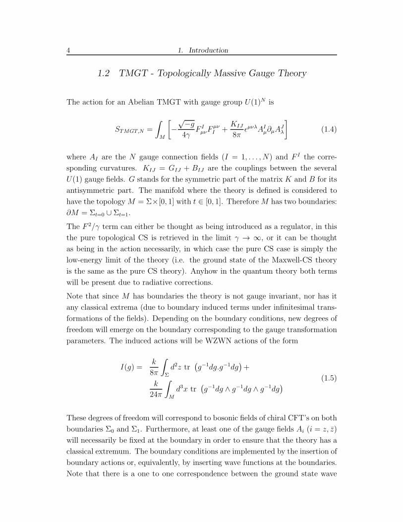
The action for an Abelian TMGT with gauge group U(1)N is
STMGT,N =
∫
M
[
−√−g4γ
F IµνF
µνI +
KIJ
8πǫµνλAI
µ∂µAJλ
]
(1.4)
where AI are the N gauge connection fields (I = 1, . . . , N) and F I the corre-
sponding curvatures. KIJ = GIJ + BIJ are the couplings between the several
U(1) gauge fields. G stands for the symmetric part of the matrix K and B for its
antisymmetric part. The manifold where the theory is defined is considered to
have the topologyM = Σ×[0, 1] with t ∈ [0, 1]. ThereforeM has two boundaries:
∂M = Σt=0 ∪ Σt=1.
The F 2/γ term can either be thought as being introduced as a regulator, in this
the pure topological CS is retrieved in the limit γ → ∞, or it can be thought
as being in the action necessarily, in which case the pure CS case is simply the
low-energy limit of the theory (i.e. the ground state of the Maxwell-CS theory
is the same as the pure CS theory). Anyhow in the quantum theory both terms
will be present due to radiative corrections.
Note that since M has boundaries the theory is not gauge invariant, nor has it
any classical extrema (due to boundary induced terms under infinitesimal trans-
formations of the fields). Depending on the boundary conditions, new degrees of
freedom will emerge on the boundary corresponding to the gauge transformation
parameters. The induced actions will be WZWN actions of the form
I(g) =k
8π
∫
Σ
d2z tr(
g−1dg.g−1dg)
+
k
24π
∫
M
d3x tr(
g−1dg ∧ g−1dg ∧ g−1dg)
(1.5)
These degrees of freedom will correspond to bosonic fields of chiral CFT’s on both
boundaries Σ0 and Σ1. Furthermore, at least one of the gauge fields Ai (i = z, z)
will necessarily be fixed at the boundary in order to ensure that the theory has a
classical extremum. The boundary conditions are implemented by the insertion of
boundary actions or, equivalently, by inserting wave functions at the boundaries.
Note that there is a one to one correspondence between the ground state wave

1.2. TMGT - Topologically Massive Gauge Theory 5
functions and the conformal blocks of the boundary CFT. It is also important
to stress that the relative boundary conditions (between both boundaries) are
selecting the kind of relative chirality of the two CFT’s, remember that the final
aim here is to obtain string theory and all the aspects inherent to it related to
CFT’s. In the case of a full non-chiral CFT, the left movers will live on one
boundary (say Σ0), while the right movers will live in the other one (Σ1).
The Maxwell term turns out to be fundamental in this construction: In the pure
CS case there are only two canonical coordinates, πz = ǫzzAz is the canonical
conjugate momenta to Az. The way to impose boundary conditions in pure CS is
to choose a proper polarizations in each boundary, which means that Az is chosen
as spatial coordinate in one boundary while Az is chosen on the other one. In the
Maxwell-CS theory there are four canonical coordinates, the canonical conjugate
momenta to Ai is πi = F 0i/γ+ kǫijAj/8π. Fixing Az only, π
z is fixed as well due
to the commutation relation [Az, πz] = 0. In this way it will indeed be possible
to have (anti)holomorphic bosonic degrees of freedom on the boundaries holding
two boundary chiral CFT’s (one in each boundary) or alternatively killing all the
degrees of freedom on only one of the boundaries allowing the construction of the
heterotic string.
The pure CS theory is geometry independent (i.e. does not depend on the met-
ric). The CS term only depends on the antisymmetric tensor, being a topological
invariant. The metric on the boundary is induced by the antisymmetric tensor
h(2)12 = ǫ012. Depending on the choice of boundary conditions (anti-holomorphic
chiral CFT’s) two inequivalent classes of metrics will be selected on the bound-
aries. Basically one is selecting a polarization of the theory, that is which of the
Ai’s is the momenta and which is the position in the phase space. By introducing
the Maxwell term the theory is made geometry dependent since F 2/√g depends
explicitly on the metric. The induced metric on the boundaries is in this case
h(2)ij = ǫ0ij/
√
g(3) for i < j.
6 1. Introduction
1.3 Topological Membrane Approach to String Theory
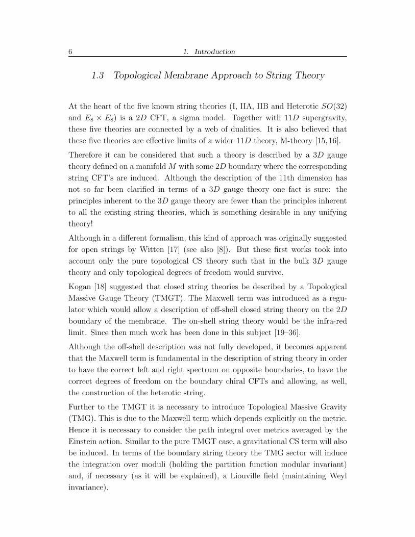
At the heart of the five known string theories (I, IIA, IIB and Heterotic SO(32)
and E8 × E8) is a 2D CFT, a sigma model. Together with 11D supergravity,
these five theories are connected by a web of dualities. It is also believed that
these five theories are effective limits of a wider 11D theory, M-theory [15, 16].
Therefore it can be considered that such a theory is described by a 3D gauge
theory defined on a manifoldM with some 2D boundary where the corresponding
string CFT’s are induced. Although the description of the 11th dimension has
not so far been clarified in terms of a 3D gauge theory one fact is sure: the
principles inherent to the 3D gauge theory are fewer than the principles inherent
to all the existing string theories, which is something desirable in any unifying
theory!
Although in a different formalism, this kind of approach was originally suggested
for open strings by Witten [17] (see also [8]). But these first works took into
account only the pure topological CS theory such that in the bulk 3D gauge
theory and only topological degrees of freedom would survive.
Kogan [18] suggested that closed string theories be described by a Topological
Massive Gauge Theory (TMGT). The Maxwell term was introduced as a regu-
lator which would allow a description of off-shell closed string theory on the 2D
boundary of the membrane. The on-shell string theory would be the infra-red
limit. Since then much work has been done in this subject [19–36].
Although the off-shell description was not fully developed, it becomes apparent
that the Maxwell term is fundamental in the description of string theory in order
to have the correct left and right spectrum on opposite boundaries, to have the
correct degrees of freedom on the boundary chiral CFTs and allowing, as well,
the construction of the heterotic string.
Further to the TMGT it is necessary to introduce Topological Massive Gravity
(TMG). This is due to the Maxwell term which depends explicitly on the metric.
Hence it is necessary to consider the path integral over metrics averaged by the
Einstein action. Similar to the pure TMGT case, a gravitational CS term will also
be induced. In terms of the boundary string theory the TMG sector will induce
the integration over moduli (holding the partition function modular invariant)
and, if necessary (as it will be explained), a Liouville field (maintaining Weyl
invariance).

1.3. Topological Membrane Approach to String Theory 7
Generic WZWN models can be built by considering appropriate bulk gauge
groups. In particular coset constructions correspond, from the point of view
of the bulk, to summing several CS actions (or more generally, TMGT actions).
Superstring theories can be built by considering supersymmetric membranes.
This can be achieved in two ways; either by considering Majorana fermions in
the bulk such that the 3D supersymmetry transformations induce fermionic edge
states (in a similar way to the gauge transformations in TMGT), or considering
an appropriate coset construction such that, on the boundary, one of the several
gauge fields that are present correspond to the bosonized fermions while the other
ones correspond to the boson fields.

8 1. Introduction
1.4 TMG - Topologically Massive Gravity
Since our action is explicitly dependent on the metric it is necessary to consider as
well a gravitational term [20, 21] and integrate over metrics in the path integral.
Note that, if this term is not present, it will be induced by quantum corrections.
The obvious candidate is the 3D Einstein action
SE = κ
∫
M
d3x√gR = κ
∫
M
d3xǫµνλǫabceaµ
(
∂νwbcλ − ∂λw
bcν + [wν , wλ]
bc)
(1.6)
where R is the curvature and both a vierbein e and a spin connection w were
introduced (gµν = eaµebνηab).
There also exists a gravitational CS term which can be thought of as induced by
quantum corrections, k′
4π
(
ηadηbcwabµ ∂νw
cdλ + 2
3ηafηbcηdew
abµ w
cdν w
efλ
)
.
The spin connection w is a function of the vierbein e. They can be made inde-
pendent by introducing a Lagrange multiplier term [20, 38].
The full TMG action is then given by
STMG =∫
Mdtd2z ǫµνλ
[
κǫabceaµ
(
∂νwbcλ − ∂λw
bcν + [wν , wλ]
bc)
+k′
4π
(
ηadηbcwabµ ∂νw
cdλ +
2
3ηafηbcηdew
abµ w
cdν w
efλ
)
+ λaµ(
ηab∂νebλ + ηabηcdw
bcµ e
dλ
)]
(1.7)
where λ in the last term is a Lagrange multiplier such that w and e are inde-
pendent and there are four canonical variables: wz, its conjugate wz, e and its
canonical conjugate βaν = λaν +
1τ2ηbdηceǫ
abcwdeν .
In 3D there is a one to one map between non-Abelian gauge theory and grav-
ity [20, 39, 40]. Define the gauge field as
Aν = eaνPa + ηcdǫabcwabν Jd (1.8)
where Ja ≡ 12ǫabcJbc, J
ab are the Lorentz generators and P a the translation gen-
erators. The gauge group corresponding to the action (1.7) is SO(2, 1) with
quadratic invariants 〈Ja, Jb〉 = 〈Pa, Pb〉 = δab and 〈Ja, Pb〉 = 0.
1.4. TMG - Topologically Massive Gravity 9
Following a similar treatment to that of the gauge theory, (gravitational) WZWN
actions with gauge group
SO(2, 1) ∼= PSL(2,C) ∼= SL(2,R)× SL(2,R) (1.9)
emerge on the boundaries of the manifold M .
It is interesting to note that similar to TMGT one can impose boundary con-
ditions such that (e.g. for the sphere) one of the SL’s is on one boundary and
the other one on the other. This means that these groups generate conformal
transformations on the boundaries. Remember that only holomorphic degrees of
freedom live on one boundary and antiholomorphic on the other one such that
conformal transformations act in z in one boundary and z in the other one.
Note that 2D ghosts do not emerge due to gauge fixing the gravitational diffeo-
morphism since the Faddeev-Popov determinant is absorbed by the constraints
of the theory (see [36] and references therein for details).
Fixing and integrating over moduli in string theory will be accomplished by con-
sidering boundary actions similarly to the method described below in section 2.1
or, equivalently, by considering the insertion of boundary wave functions as de-
scribed below in section 2.2 for the gauge sector.
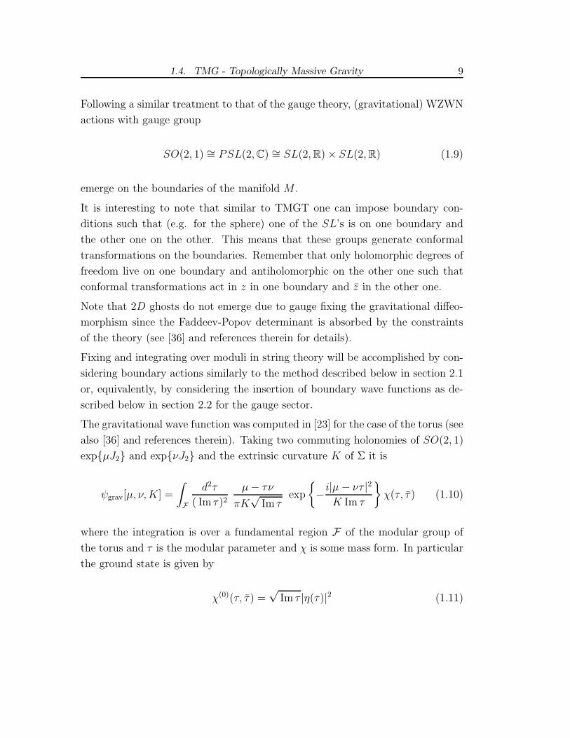
The gravitational wave function was computed in [23] for the case of the torus (see
also [36] and references therein). Taking two commuting holonomies of SO(2, 1)
expµJ2 and expνJ2 and the extrinsic curvature K of Σ it is
ψgrav[µ, ν,K] =
∫
F
d2τ
( Im τ)2µ− τν
πK√
Im τexp
−i|µ − ντ |2K Im τ
χ(τ, τ) (1.10)
where the integration is over a fundamental region F of the modular group of
the torus and τ is the modular parameter and χ is some mass form. In particular
the ground state is given by
χ(0)(τ, τ) =√
Im τ |η(τ)|2 (1.11)

10 1. Introduction
with η(τ) the usual Dedekind eta function
η(τ) = exp 2πiτ/24∞∏
r=1
(1− exp 2πirτ) (1.12)
Computing the ground state to ground state transition amplitude one finds
⟨
ψ(0)grav|ψ(0)
grav
⟩
=
∫
F
d2τ
( Im τ)2|η(τ)|4 (1.13)
This is exactly the diffeomorphism ghost contribution for the partition function
of string theory when the moduli are gauge fixed (for the torus).
These computations have not been performed for higher genus Riemann surfaces
but a similar picture should hold.
What remains is to explain how the Liouville field emerges from TMG. To do so
consider the gravitational WZWN model induced at the boundaries due to the
diffeomorphisms
I(g, w) =k′
4π
∫
Σ
d2z tr(
g−1dg.g−1dg)
+
k
12π
∫
M
d3x tr(
g−1dg ∧ g−1dg ∧ g−1dg)
+
k′
4π
∫
Σ
d2z tr(
2w.g−1dg − 2Mwa.ea + w.w)
(1.14)
where M = 2πκ/k′ stands for the mass of the 3D bulk graviton.
The previous discussion generating the ghost concerns the ground state of the
theory, or equivalently, the topological limit of the theory. This topological limit
corresponds to the vacuum expectation values of the driebeins being zero, 〈eaν〉 =0. In the case that this value is taken to be non-zero
〈eaν〉 = δaν (1.15)
the bulk graviton becomes massive and the boundary theories are not diffeomor-
phism invariant any longer.

1.4. TMG - Topologically Massive Gravity 11
The full computation is done in [36] and is not going to be carried out here. It is
enough to consider the Gauss decompositions for the SL(2,R) group introduced
in [41]
g =
1 0
γ 1
eφ 0
0 e−φ
1 γ′
0 1
(1.16)
After an appropriate redefinition of φ one gets the Liouville action on the 2D
boundary with a cosmological constant µ
SLiouv =
∫
Σ
d2z(
∂zφ∂zφ+ λR(2)φ+ µ exp βφ)
(1.17)
where β and λ are appropriate constants used in the redefinition of φ.
Furthermore the 2D cosmological constant turns out to be exactly the square of
the graviton mass
µ =M2 (1.18)
The interesting conclusion to draw from the previous discussion is that the bulk
theory, in the topological limit of TMG reproduces Weyl and conformal invari-
ance and gives us the appropriate ghosts and integration over moduli space. Once
one considers excited states the boundary theory is not Weyl invariant anymore;
instead a new field, identified with the boundary Liouville field, emerges such
that the total boundary action is again Weyl invariant. Note that this mecha-
nism is exactly the one in string theory which gives rise to a new target space
coordinate, the Liouville field (see for instance [42] for this discussion), but is here
obtained from TMG arguments! This is actually one way of getting an extra 11th
dimension.
Note that this argument is very similar to the discussion concerning TMGT when
considering strings off-shell. In the topological limit (ground state) one obtains
the usual on-shell string CFT on the boundaries, while when considering excited
states one obtains a non-conformal theory on the boundaries corresponding to
off-shell string theories.
To finalize this discussion note that the mechanism just described is simply forcing
the boundary theory to be critical. This means the total central charge is zero
and one obtains critical string theory.

12 1. Introduction
1.5 Supersymmetry
In order to generate superconformal boundary actions one may take two different
approaches. Either consider a bulk fermionic sector such that the 3D theory is su-
persymmetric and the supersymmetry transformations induce on the boundaries
the correct superconformal degrees of freedom [24,28], or it may be considered as
a coset model such that one of the gauge fields represent bosonized fermions and
the other fields are responsible for the flux between different sectors (i.e. between
the boundaries), say Ramond and Neveu-Schwarz for example [30].
Consider the 3D supersymmetric massive gauge action
S =
∫
M
[
− 1
4γFµνF
µν +k
8πǫµνλAµ∂νAλ +
1
2γΨγµ∂µΨ− k
8πΨΨ
]
(1.19)
with Ψ = (ψ, ψ) being a two-component Majorana-Weyl fermion.
As for the TMGT case, due to the boundaries, the action does not have an
extremum and is not invariant under the bulk N = 1 supersymmetry transfor-
mations
δAµ = η (∂µλ− γµψ)
δψ = ǫµνλ∂νAλγµη
(1.20)
where η is a global Grassmann parameter. Note that the first term in the trans-
formation of A can be thought as a gauge transformation with parameter ηλ.
In each boundary one can impose one of the components of Ψ to be fixed such that
a chiral action is generated. On each boundary only N = 1/2 supersymmetry
will survive such that upon identifying both boundaries the resulting non-chiral
world-sheet action will correspond to N = 1 supersymmetry.
As an example the NSR string action
SNSR =k
8π
∫
Σ
d2x[
∂zX∂zX − iψγµ∂µψ]
(1.21)
can be obtained by taking ψ fixed in Σ0 and ψ fixed in Σ1 and adding the
boundary action k/8π(
∫
Σ0
ψ∂zψ −∫
Σ1
ψ∂zψ)
. For a more detailed calculation
see for instance the similar computation carried out for the TMGT sector in
section 2.1 [24].

1.5. Supersymmetry 13
Consider now the second proposed approach using coset constructions. To gen-
erate the supersymmetric Virasoro algebra on the 2D boundary WZWN model
corresponding to the N = 2 superconformal minimal model, the coset to be
considered is [30]
Mk = SU(2)k+2/U(1)k+2 ≡ SU(2)k × SO(2)2/U(1)k+2 (1.22)
In terms of the bulk theory this corresponds to the action:
SMk= kISU(2) + 2ISO(2) − (k + 2)IU(1) (1.23)
The central charge of this minimal model is
ck =3k
k + 2(1.24)
The TMGT corresponding to the Abelian gauge group SO(2) will induce on the
boundary a 2D action which, upon fermionization, is the worldsheet fermionic
sector of the superstring. Its ground state solution is degenerate. At level l
there are l/(2η2)g solutions, where g is the genus of the Riemann surface Σg.
The matter is introduced in the theory through closed Wilson lines carrying half
integer charges Qη = 1/2 corresponding to Fermi statistics, the wave function for
a gauge field B is
Ψrl = exp
[
− 1
16πblτlm(b− b)m
]
Θg
r/4
0
(
b
π
∣
∣
∣
∣
8τ
π
)
(1.25)
with the decomposition B = b+dφ+∗dχ, where b = (blωl−blωl). The indices run
l, m = 1, . . . , g and rl = 1, 2, 3, 4(≤ l/2η2). τ is a g× g matrix which encodes the
modular structure of Σg and ωl = bαl + τlmbβm is parameterized by the harmonic
forms bα and bβ normalized as the Poincare duals∮
αmbαl =
∮
βmbβl = δml and
∮
αmbβl =
∮
βmbαl = 0. The closed contours α and β stand for a basis of the
canonical homology cycles of the Riemann surface Σg.
The boundary states of the 3D theory corresponding to the NS and R sectors

14 1. Introduction
are obtained as quantum superimpositions of the 4 possible ground states |rl〉,which is to say that the correct basis of states will be chosen. The periodicity
on both worldsheet coordinates can be measured in the TM framework using the
Wilson loop operators WC [B] = exp[
iQη
∮
CB]
by taking C to be a fixed time
path coinciding with the holonomy cycles of Σg
W lα = exp[i(b− b)l] W l
β = exp[i(τlmbm − τlmb
m)] (1.26)
The averages of these operators are 〈Wi〉 = ±1 (i = α, β) corresponding to peri-
odic (+1) and antiperiodic (−1) fermions. For genus 1 the results are summarized
in table 1.1.
Ψ 〈Wα〉 〈Wβ〉 type|1〉+ |3〉 + − R|1〉 − |3〉 − − NS|2〉+ |4〉 + + R|2〉 − |4〉 − + NS
Tab. 1.1: Ground state superpositions holding NS and R periodicities for genus 1.
The GSO projections emerge in this way as the sum over these ground states.
This is equivalent to projecting the trace in the partition function onto states
with eigenvalue +1 of the Klein operator (−1)F (states with an even number
of fermions). This is actually the mechanism which ensures that string theory
is modular invariant and that the 10D target space theory of string theory is
supersymmetric.
To end this Chapter note again that the full supersymmetric TM induces 10D
critical string theories. But if one considers the full TM, including TMG as well,
the 11D may be generated through the Liouville field and/or the superghosts [43].

2. QUANTIZATION OF TMGT
2.1 Path Integral Formalism
There are several ways to derive CFT from CS theory. The path integral approach
was first suggested by Ogura [13] (see also [22]). In this section we review some
features of TMGT defined on a three dimensional flat manifold with a boundary.
In order to clarify, some arguments derived from canonical formalism are present
although the full canonical quantization will only be carried in the next section.
A list of the induced chiral boundary conformal field theories is presented and
a careful analysis of the Gauss law structure is considered such that the charge
spectrum of the theory is built.
Two kind boundary conditions on the gauge fields will be considered in the re-
maining of this work. Either the fields of the theory are constraint (are compact)
in such a way that large gauge transformations are allowed or not. They will be
labeled by B and B:
B : Gauge transformations are allowed
B : Gauge transformations are not allowed(2.1)
Similarly to the action (1.4), the TMGT action for a single U(1) gauge group
obeying B boundary conditions is
STMGT,1 =
∫
M
d2z dt
[
−√−g(3)4γ
F µνFµν +k
8πǫµνλAµ∂νAλ
]
(2.2)
where M = Σ× [0, 1] and Σ is a 2D compact Euclidean manifold with a complex
structure denoted by (z, z). The time-like coordinate takes values in the compact

16 2. Quantization of TMGT
domain t ∈ [0, 1]. The indices run over µ = 0, i with i = z, z.
Under an infinitesimal variation of the fields A→ A+ δA the action changes by
δS =
∫
M
(√−g(3)γ
∂µFµν +
k
4πǫµλν∂µAλ
)
δAν −[∫
Σ
ΠiδAi
]t=1
t=0
(2.3)
where
Πi =1
γF 0i − k
8πǫijAj (2.4)
is the canonical momentum conjugate to Ai. Note that the 2D antisymmetric
tensor ǫij is induced by the 3D antisymmetric tensor and metric
ǫij =−ǫ0ij√−g(3)
(2.5)
When referring to the usual 2D antisymmetric tensor the notation ǫij (without
the tilde) is used [63].
In order for the theory to have a classical extremum it is necessary to impose
suitable boundary conditions for which the second term in the variation of the
action vanishes. Let us assume that the boundary of M has two pieces, which
are Σ(t=0) = Σ0 and Σ(t=1) = Σ1. On each of the boundaries, up to gauge
transformations, one can fix one or both fields Az and Az. In doing so it is
necessary to add an appropriate boundary action SB = SB0 + SB1 such that the
new action S + SB has no boundary variation, and hence well defined classical
extrema. Note that upon canonical quantization it is necessary to impose the
corresponding equal time commutation relations of Π and A
[Πi(z), Aj(z′)] = gijδ(2)(z− z′) (2.6)
The convention for the metric used here is gzz = gzz = 2. So upon fixing Az, Πz
is fixed as well. The same holds for the Az and Πz components.
Then, on each component of the boundary (∂M = Σ0 ∪ Σ1) the possible choices

2.1. Path Integral Formalism 17
of boundary conditions and boundary actions are
boundary conditions Σ1 bound. action Σ0 bound. action
N. δAz = δAz = 0 SB1 = 0 SB0 = 0
C. δAz = 0 SB1 =
∫
Σ1
ΠzAz SB0 = −∫
Σ0
ΠzAz
C. δAz = 0 SB1 =
∫
Σ1
ΠzAz SB0 = −∫
Σ0
ΠzAz
(2.7)
There are nine allowed choices: NN , NC, CC, CC, and so on. The first letter
denotes the type of boundary conditions on Σ0 and the second one on Σ1. The
N boundary condition stands for Non-Conformal or Non-Dynamical, C stands
for Conformal and C for anti-Conformal and are related to the kind of CFT
which are obtained on the boundaries when each of them are chosen, basically
if the bosonic fields are holomorphic or antiholomorphic. Note the importance
of the F 2 term, it gives the theory four independent canonical coordinates, as
opposed to the two of the pure Chern-Simons theory (where one of the A’s is
canonically conjugate to the other). This fact allows us to fix both of the A’s and
corresponding Π in the same boundary allowing the construction of the heterotic
string. For further details we refer the reader to [24, 28]. This topic will be
addressed again in section 3.3.
But note that even with the addition of these boundary actions the full action
is not invariant under gauge transformations. Considering the transformation
A→ A+ dΛ, the bulk action transforms as
S → S − k
8π
[∫
Σ
ǫij∂iΛAj
]t=1
t=0
(2.8)
while the boundary actions transform as
ΠzAz → ΠzAz +Πz∂zΛ− k
8πǫzz∂zΛAz −
k
8πǫzz∂zΛ∂zΛ (2.9)

18 2. Quantization of TMGT
This fact is actually what makes possible the construction of effective 2D bound-
ary theories out of 3D ones. The gauge parameters will constitute the degrees of
freedom of those 2D theories. To see it explicitly consider gauge fixing the path
integral by Faddeev-Popov procedure such that Aµ = Aµ + ∂µΛ. The action and
path integral factorize as
Z =
∫
DA∆FP δ(
F (A))
eiS[A]
∫
DλDχeiSB[χ,λ] (2.10)
where on the boundaries the gauge parameters Λ(t = 0) = χ and Λ(t = 1) = λ
become dynamical degrees of freedom which decouple from the bulk theory.
As an example take CC boundary conditions. After gauge fixing the boundary
action becomes
SB,CC =
∫
Σ1
[
ΠzAz + Πz∂zλ− k
8πǫzz∂zλAz −
k
8πǫzz∂zλ∂zλ
]
−∫
Σ0
[
ΠzAz + Πz∂zχ +k
8πǫzz∂zχAz +
k
8πǫzz∂zχ∂zχ
] (2.11)
Gluing both boundaries using the identification z ∼= z and Az∼= Az the previous
action can be rewritten in the simpler form
SB,CC =
∫
Σ
[
(Πz − k
8πǫzz∂zλ)(Az + ∂zχ)− (Πz − k
8πǫzz∂zχ)(Az − ∂zλ)
− k
8πǫzz∂z(χ− λ)∂z(χ− λ)
]
(2.12)
where Σ stands for the identified Σ0∼= Σ1.
In the path integral there is still a dependence on the boundary values of A’s.
Assuming that the measure can be factorized into a bulk integration times a
boundary integration
∫
DAzDAz =
∫
DAz,bulkDAz,bulk
∫
DAz,boundDAz,bound (2.13)

2.1. Path Integral Formalism 19
and performing the Gaussian integration on the boundary A’s one gets the action
SB =k
4π
∫
gij∂i(χ− λ)∂j(χ− λ) (2.14)
presented in the second factor of (2.10). The metric is identified as gzz = −i2ǫzz.Note that ǫzz = i.
This action can be recognized as the d = 1 free boson action∫
∂X∂X with
X = χ−λ. χ stands for the holomorphic part of X and λ for the antiholomorphic
part. The point to stress is that it completely decouples from the bulk and the
path integral indeed factorizes. In this way it is proved that there is actually an
effective 2D boundary CFT.
Note that the effective boundary action depends on the chosen boundary con-
ditions and the identifications used in the gluing procedure. This issue will be
dealt with in more detail in section 3.3.
Now let us find the allowed charges in this theory. The boundary conditions
of the gauge fields A has to be taken into account and it turns out to be of
fundamental importance due to the existence of large gauge transformations (for
compact A) around the holonomies of the gauge connections. Define the electric
and magnetic fields as
Ei =1
γF 0i = Πi +
k
8πǫijAj
B = ǫij∂iAj
(2.15)
The commutation relations follow directly from the Poisson bracket and read
[Ei(z), Ej(z′)] = −i k4πǫijδ(2)(z− z′)
[Ei(z), B(z′)] = −iǫij∂jδ(2)(z− z′)
(2.16)
If there is an external charge ρ0 (coupled to A0 in the action), the Gauss law
is imposed by integrating the field component A0 in the path integral and reads
simply
∂iEi +
k
4πB = ρ0 (2.17)

20 2. Quantization of TMGT
In the quantum theory this equation needs to be satisfied by the physical states.
So, following [26], the generator of time independent gauge transformations U
can easily be defined as
U = exp
i
∫
Σ
Λ(z)
(
∂iEi +
k
4πB − ρ0
)
(2.18)
where Σ stands for a generic fixed time slice of M . Since the gauge fields are
compact, Λ is identified with (mapped to) an angle in the complex plane such
that
ln(z) = ln |z|+ i(Λ(z) + 2πn)
∂iΛ(z) = −ǫij∂j ln |z|(2.19)
where the second equation follows from the Cauchy-Riemann equations. This
last condition on Λ will restrict the physical Hilbert space of the theory [54–57].
Let us define a new local operator
V (z0) = exp
−i∫
Σ
d2z
[(
Ei +k
4πǫijAj
)
ǫik∂k ln |z0 − z| − Λ(z0 − z)ρ0
]
(2.20)
The physical states of the theory must be gauge invariant (under U) as well as
eigenstates of this new local operator. Using the identity ∂k∂k ln |z| = 2πδ(z) and
the commutation relations (2.16) for E and B is obtained the relation
[B(z), V n(z0)] = 2πnV n(z0)δ(2)(z− z′) (2.21)
This means that the operator V creates a pointlike magnetic vortex at z0 with
magnetic flux∫
Σ
B = 2πn n ∈ Z (2.22)
Note that this operator only exists in the gauge theory where the boundary
conditions on the fields are such that allow large gauge conditions. If one wants
to enlarge the gauge group to include a non-compact gauge field sector (as will be
discussed below) these quantum operators and the induced quantum transitions
induced by them will not be present in that sector. Also, as stated before the
F 2 term is fundamental for the existence of these tunneling processes that hold

2.1. Path Integral Formalism 21
local charge non conservation, see [44,54] for further details. Instantons in three
dimensions are the monopoles in four dimensions. So in the rest of the manuscript
they will be called either instanton and monopole without any distinction.
Using the functional Schrodinger representation Πi = iδ/δAi and imposing the
condition that phase acquired by a physical state under a gauge transformation
be single valued the charge spectrum is obtained
q = m+k
8π
∫
Σ
B = m+k
4n m, n ∈ Z (2.23)
As it can be seen from the above formula for a generic, non-integer, value of k the
allowed charges are non-integers. In principle in the Abelian theory one expects
that the charges are quantized as happens in the Maxwell theory. But the exis-
tence of the Chern-Simons term changes this picture, the charges are quantized
through m and n dependence but here k itself is considered not to be quantized
(this point of view differs from many other works in the subject). As will be
explained below this fact is only compatible with (and demands) the existence of
a new gauge sector which fields do not allow large gauge transformations.
A charge q propagating in the bulk can interact with one monopole with flux (2.22)
changing by an amount
∆q =k
2n (2.24)
The path of a charge in the bulk can be thought as a Wilson line. The phase
induced by the linking of two Wilson lines carrying charges q1 and q2 is
< Wq0Wq1 >= exp
2πi2
kq0 q1 l
(2.25)
where l is the linking number between the lines. The above computation was
done in the limit of vanishing Maxwell term and with the assumption that there
is no self-linking for the individual Wilson lines. The connection between the
boundary CFT’s and the bulk theory can be achieved by noting that the bulk
gauge fields become pure gauge in the boundary and the Wilson lines on the
boundary are none other than the vertex operators on Σ0 and Σ1 with momenta

22 2. Quantization of TMGT
q
V0,q0 = exp
−iq∫
Aνdxν∣
∣
Σ0
= exp −iq0λ
V1,q1 = exp
−iq∫
Aνdxν∣
∣
Σ1
= exp −iq1χ(2.26)
Note that generally, as will be considered in the next chapter, the charge q figuring
in the Wilson line is not constant and may change over time due to tunneling
effects, i.e. monopole processes.
The conformal dimensions of these vertices are
∆0 =q20
k
∆1 =q21
k
(2.27)
k appears because the induced action on the boundary is that of a chiral string
action multiplied by k such that it plays the role of the (inverse) Regge slope and
has dimensions of (target) space-time. To see the Wilson line and vertex operator
correspondence let us obtain the above result from the bulk theory. Consider two
Wilson lines carrying charges q and −q propagating from one boundary to the
other corresponding to two vertex insertions on the boundary with momenta q
and −q, see figure (2.1).
Two point correlation functions of these two vertices follows as usual
< V0,q(z1)V0,−q(z2)) >=1
z122∆
< V1,q(z1)V1,−q(z2)) >=1
z2∆12
(2.28)
A rotation of one charge (vertex) around the other in one boundary induces a
phase of −4πi∆ in (2.28). In the bulk this rotation induces one linking of the
Wilson lines (l → l + 1), so (2.25) gives an Aharonov-Bohm phase change of
−4πiq2/k. By identifying these two phases it is concluded that (2.27) follows.
Let us recall that in terms of the three dimensional theory Polyakov [58] pointed
out that ∆ is the transmuted spin of a charged particle which exists because of
the interaction with the Chern-Simons term. So the conformal dimension of the
boundary fields is identified with the transmuted spin of the bulk charges. For

2.1. Path Integral Formalism 23
Fig. 2.1: Two charges propagating through the bulk are represented as two Wilson lines,By a rotation of one charge around the other one, a linking (l = 1) is induced in thebulk.
later use let this result be generalized to three charges q1, q2 and q3 = −q1 − q2.
The net charge will always be considered to be zero. The correlation function of
three vertices reads
< Vq1(z1)Vq2(z2)Vq3(z3)) >=1
z12∆1+∆2−∆3z13∆1+∆3−∆2z23∆2+∆3−∆1
(2.29)
where the charge-conformal dimension identifications are
∆1 +∆2 −∆3 = − 2kq1q2
∆1 +∆3 −∆2 = 2kq1(q1 + q2)
∆2 +∆3 −∆1 = 2kq2(q1 + q2)
(2.30)
The antiholomorphic three point correlation function follows trivially.
It is clear that if any one of the vertices is rotated around one of the other two;
the phase factor induced in the three-point function will be the same as (2.25)
which comes from the linking of Wilson lines in the bulk. From the point of
view of CFT the sum of conformal factors must be integer in order to have single

24 2. Quantization of TMGT
valued OPE’s. This result is going to be derived from the bulk theory in the next
section independently of the boundary. By a simple argument let us show that
there can exist only integer conformal dimensions for each vertex. At the level
of the two point correlation functions there can exist two integer ∆’s or two half
integer ∆’s. For three point functions it is necessary to have three integer ∆’s
or two integer and one half integer ∆’s. One can then consider the four point
function and decompose it to two pairs which are well separated from each other.
In this case the conformal dimensions can be integers and half-integers. Suppose
that at least two of the vertices have half-integer conformal dimensions. Then
one vertex from a pair can be adiabatically moved to the other pair and a three
point function with a total half-integer conformal dimension will be formed. But
this is not permitted as argued above. For this reason the existence of vertices
with half integer conformal dimension is excluded. The same arguments follow
for the charges from the point of view of the 3D bulk theory.
Let us remember that there are two independent chiral conformal field theories
on two different surfaces up to this point. In order to get a non-chiral CFT (as
in string theory) is necessary to identify in some way the two boundaries. The
most obvious way to define non-chiral vertex operators is
Vq0,q1(z, z) = V0,q0(z)V1,q1(z) (2.31)
with the conformal dimension
∆0 +∆1 =1
k(q20 + q21) (2.32)
As long as V0 is considered to be holomorphic and V1 antiholomorphic or vice-
versa, the full vertex is indeed non-chiral.
Note that there is a little bit of difference in the nomenclature in relation to
the standard one. In most of the literature ∆0 = ∆ and ∆1 = ∆ are called
conformal weights, ∆ − ∆ is called the spin and the sum (2.32) ∆ + ∆ is called
the conformal dimension. Here ∆ and ∆ are called conformal dimensions as well
when referring to the chiral vertices operators since they can exist in each of
the boundaries independently of each other. From now on the notation will be
definitively changed to ∆ = ∆0 and ∆ = ∆1 and the same for the charges, q0 = q
and q1 = q.
2.2. Canonical Formalism 25
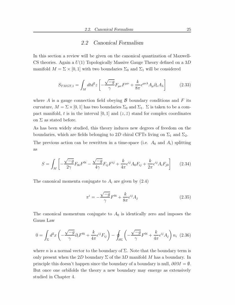
2.2 Canonical Formalism
In this section a review will be given on the canonical quantization of Maxwell-
CS theories. Again a U(1) Topologically Massive Gauge Theory defined on a 3D
manifold M = Σ× [0, 1] with two boundaries Σ0 and Σ1 will be considered
STMGT,1 =
∫
M
dtd2z
[
−√−gγ
FµνFµν +
k
8πǫµνλAµ∂νAλ
]
(2.33)
where A is a gauge connection field obeying B boundary conditions and F its
curvature, M = Σ× [0, 1] has two boundaries Σ0 and Σ1. Σ is taken to be a com-
pact manifold, t is in the interval [0, 1] and (z, z) stand for complex coordinates
on Σ as stated before.
As has been widely studied, this theory induces new degrees of freedom on the
boundaries, which are fields belonging to 2D chiral CFTs living on Σ1 and Σ2.
The previous action can be rewritten in a time-space (i.e. A0 and Ai) splitting
as
S =
∫
M
[
−√−g2γ
F0iF0i −
√−g4γ
FijFij +
k
4πǫijA0Fij +
k
2πǫijAiFj0
]
(2.34)
The canonical momenta conjugate to Ai are given by (2.4)
πi = −√−gγ
F 0i +k
8πǫijAj (2.35)
The canonical momentum conjugate to A0 is identically zero and imposes the
Gauss Law
0 =
∫
Σ
d2x
(
−√−gγ
∂iF0i +
k
4πǫijFij
)
−∮
∂Σ
(
−√−gγ
F 0i +k
4πǫijAj
)
ni (2.36)
where n is a normal vector to the boundary of Σ. Note that the boundary term is
only present when the 2D boundary Σ of the 3D manifold M has a boundary. In
principle this doesn’t happen since the boundary of a boundary is null, ∂∂M = ∅.But once one orbifolds the theory a new boundary may emerge as extensively
studied in Chapter 4.

26 2. Quantization of TMGT
The Hamiltonian of the theory is computed to be
H = Πi∂0Ai − L =
= −A0
[
∂i
(
πi − k
4πǫijAj
)
+k
8πǫijFij
]
+ ∂i(A0πi)
+
√−g16γ
(ǫijFij)2 +
γ
2hij
(
πi − k
8πǫikAk
)(
πj − k
8πǫjlAl
)
(2.37)
As usual A0 can be considered to be a Lagrange multiplier which imposes the
Gauss law.
The electric and magnetic fields are defined as in (2.15)
Ei =1
γF 0i
B = ∂zAz − ∂zAz
(2.38)
and the Gauss law (without boundary terms) reads simply
∂iEi +
k
4πB = ρ0 (2.39)
as already given in (2.17)
Upon quantization the charge spectrum is
Q = m+k
4n (2.40)
for some integersm and n. Furthermore, it has been proved [26,29] that under the
correct relative boundary conditions, one insertion of Q on one boundary (cor-
responding to a vertex operator insertion on the boundary CFT) will necessarily
demand an insertion of the charge
Q = m− k
4n (2.41)
on the other boundary. This statement is going to be derived in chapter 3 and will
be assumed through out the rest of this section. Some hints on how to rederive
2.2. Canonical Formalism 27
these results from a canonical perspective are given in this section which is based
on work in progress [92].
2.2.1 Wave Function as Boundary Conditions
The functional approach of [63] is followed next in order to derive the wave
functions of the theory.
The functional Gauss law constraint takes the form
[
Dz
(
−i δ
δAz+
k
8πǫzzAz
)
+Dz
(
−i δ
δAz− k
8πǫzzAz
)
+k
4πǫzzFzz
]
Ψ[Az, az] = 0
(2.42)
In TMGT the wave functions are not gauge invariant, as they transform with a
one-cocycle. The way to make them gauge invariant is to integrate the cocycle
condition such that they decompose into three factors
Ψ[Az, Az] =
− ik
4π
∫
d2z√hǫzzAzAz
ψ[Az]Φ[B] (2.43)
where B = ∂zAz − ∂zAz is the magnetic field and ds2(3) = gijdxidxj = −dt2 +
hzzdzdz. From now on the metric is fixed to be of this form with hzz = 1 (the
TMG sector is not considered). Note that√−g = −i and the 2D antisymmetric
tensor ǫ is purely imaginary and induced from the bulk by ǫij = ǫ0ij√−g
such that
ǫzz = i.
The factor Φ[B] is the solution for the pure Maxwell theory such that the Gauss
law constraint is obeyed
[
Dzδ
δAz+Dz
δ
δAz
]
Φ = 0 (2.44)
For further details in the treatment of this factor see [63] and references therein.
If the fields have nontrivial magnetic charge∫
B 6= 0 the wave function is 0.
Note that this result is the statement of overall charge conservation on the closed
surface one is considering. Of course it is possible that non-zero magnetic field
distributions exist locally.
ψ[Az] is a topological term (due to the Chern-Simons term in the Lagrangian)

28 2. Quantization of TMGT
and obeys the Schrodinger equation
[
Dzδ
δAz
− ik
4πǫzz∂zAz
]
ψ[Az] = 0 (2.45)
Note that this equation corresponds in the topological limit (the ground state),
with Φ = 1, to the equation in Ψ
[
Dzδ
δAz+
k
8πDzAz −
k
4πFzz
]
Ψ[A]|CS = 0 (2.46)
where 2D Euclidean space-time is considered with ǫzz = i.
As presented in [17] one solution of (2.46) for some fixed time t, compatible with
WZWN construction for an Abelian gauge group, is
Ψ[A] =
∫
Dφ exp
k
8π
∫
Σ(t)
[
AzAz − 2Az∂zφ+ ∂zφ∂zφ]
(2.47)
Here it is enough to consider the lowest Landau level (the ground state) of the
theory since it is the most probable state. This means the topological limit is
being considered, in which case Φ = 1 and the solution for the pure Chern-Simons
case is retrieved. This solution corresponds to configurations with weak magnetic
field, ǫzzFzz ≃ 0. Nevertheless it is important to stress that here Az and Az are
not canonically conjugate variables, unlike the pure CS case.
Next it will be shown that these wave functions are the building blocks of the
boundary theories; by inserting such states on the boundaries they act as bound-
ary conditions and are effectively selecting our boundary world. In this way,
through φ, new degrees of freedom are inserted on the boundaries. Furthermore,
these wave functions are necessary for the consistency of the full theory (in a
bounded manifold) as a well-defined gauge theory. Basically they play the same
role as the actions inserted on the boundary of the previous section.
Consider, for the time being, two states of the form (2.47) inserted at the bound-
aries Σ(t = 0) and Σ(t = 1). The partition function is then the correlator
Z = 〈Ψ0|Ψ1〉 =∫
DAzDAzeiSΨ0Ψ1 (2.48)

2.2. Canonical Formalism 29
where Ψ1 is given by (2.47) with Σ(t) = Σ1 while Ψ0 is
Ψ0[A] =
∫
Dφ exp
k
8π
∫
Σ0
[
−AzAz + 2Az∂zφ− ∂zφ∂zφ]
(2.49)
The overall minus sign comes from the change z ↔ z in the measure of the
integral due to the change of relative orientations from boundary to boundary.
The importance of the insertion of these boundary wave functions is that they
constrain the theory assuring that the path integral (2.48) is both, gauge invariant
and has a classical extremum.
Performing a gauge transformation Ai → Ai + ∂iΛ, the bulk exponential factor
in the partition function (similarly to (2.8)) changes as
S → S − k
8π
∫
Σ
d2z [Az∂zΛ−Az∂zΛ]
∣
∣
∣
∣
Σ1
Σ0
(2.50)
where, as in (2.46), a Euclidean 2D structure was taken. Here is where the non
gauge invariance due to boundaries resides. Taking the transformation of the one
on Σ1 gives
k
8π
∫
Σ1
[
AzAz − 2Az∂zφ+ ∂zφ∂zφ]
→
k
8π
∫
Σ1
[AzAz + Az∂zΛ + ∂zΛAz + ∂zΛ∂zΛ −2Az∂zφ− 2∂zΛ∂zφ+ ∂zφ∂zφ]
(2.51)
Combining all the factors, the exponential factor corresponding to Σ1 is simply
k
8π
∫
Σ1
[
AzAz − 2Az∂z(φ− Λ) + ∂z(φ− Λ)∂z(φ− Λ)]
(2.52)
The gauge parameter Λ is now easily eliminated by redefining the field corre-
sponding to the degree of freedom at the boundary, φ → φ+Λ. This redefinition
does not change the measure Dφ. In this elegant way, by inserting ad hoc new
degrees of freedom one manages to ensure gauge invariance of the full theory. An-
other way to explain things is that gauge transformations will necessarily induce
new degrees of freedom on the boundaries as argued in the last section. Both

30 2. Quantization of TMGT
ways of arguing are equivalent.
Further to this discussion, the boundary wave functions ensure that the theory has
a classical extremum. An infinitesimal variation of the fields induce exponential
boundary terms of the form
iδS∂M =ik
8π
∫
Σ1
ǫijAiδAj −ik
8π
∫
Σ0
ǫijAiδAj (2.53)
After a change of measure to ∂zφ and ∂zφ the integrals on the boundary can be
performed resulting in terms of the form
∫
D(∂zφ(1)∂zφ(0))δΣ1(2Az−∂zφ)δΣ0
(2Az−∂zφ) exp
k
8π
∫
Σ1
AzAz −k
8π
∫
Σ0
AzAz
(2.54)
In this way Az is fixed on one boundary while Az is fixed on the other boundary
such that δAz|Σ1= 0 and δAz|Σ0
= 0. The net boundary variation containing
δAi vanishes since the term which comes from the bulk cancels the one coming
from boundary exponential term in the wave functions. In this way the theory
has a well defined classical limit. Note as well that the fields φ living on Σ0
correspond to holomorphic degrees of freedom while the ones living on Σ1 are
antiholomorphic. It is with this construction that the two chiral CFT’s on the
boundary are obtained.
2.2.2 Conformal Blocks and the CFT Partition Function
Turning to specific geometries, consider a Hodge decomposition of the gauge fields
Ai at each time slice A = a+ dφR + ∗dφI such that
Az = az + ∂zφ
Az = az + ∂zφ
(2.55)
where φ = φR + iφI is a complex scalar field and a is a harmonic form, da =
∗da = 0 such that ∂zaz ± ∂zaz = 0.
For a torus with modular parameter τ = τ1 + iτ2 the parameterization for the

2.2. Canonical Formalism 31
harmonic form is
az = πiaτ−12 ω(z)
az = −πiaτ−12 ω(z)
(2.56)
τ2 is the imaginary part of τ . ω is an holomorphic one-form such that∫
αω = 1,
∫
βω = τ and
∫
d2zωω = −2iτ2. α and β are closed non contractible contours in
the torus which generate its first homology. Considering this parameterization
and the rational k = 2p/q (with even p), one can build an orthonormal basis with
pq elements for the wave functions [11]
Ψ0,λ = C exp
kπ
4aτ−1
2 (a− a)
Θ
λq
0
(√2a|2τ
k
)
(2.57)
with λ = 0, 1, . . . , pq − 1 and Θ are modified Jacobi theta-functions
Θ
λq
0
(√2a|2τ
k) =
∑
s∈Z
exp
2πiτ1
k
(
sp+λ
q
)2
+ 2√2πia
(
sp+λ
q
)
(2.58)
where the sum is considered to run only over multiples of p (it is in this sense it
was called modified). Note the different normalization compared to reference [11].
There Bos and Nair considered the Chern-Simons coefficient to be k = 2p′q
(p = 2p′). Taking the normalization used here the U(1) charges carried by Wilson
lines have to belong to the spectrum of the theory as given by (2.40). In this way
large gauge transformations, a→ a+s+τr, are restricted to the ones which have
s, r = 0mod p. Note that λ/q are the primary charges and that for rational values
of k there is one charge independent monopole process corresponding to ∆Q = p.
In terms of the CFT these shifts of charge are inside the same family as will be
shown in section 3.4. Then the above restriction on large gauge transformations is
nothing else then the allowed monopole processes which shifts the charges inside
the same family or block. The remaining numerical factors in the Θ functions
come from the factor k/8π instead of k/4π.
As has been widely studied [11,12] there is a one-to-one correspondence between
the 3D QFT wave functions and the blocks of the 2D CFT. In this work the
wave functions are interpreted as being labeled by charges in such a way that,

32 2. Quantization of TMGT
again, there is a one-to-one correspondence between the primary charges of the
theory (or each family of charges) and the wave functions (and necessarily the
conformal blocks).
Consider the pair (m,n) (obeying the Bezout lemma) such that for a given pri-
mary charge λ/q = m + kn/4 on one boundary, as will be derived in detail in
section 3.2, there will be a corresponding charge λ/q = m − kn/4 on the other
boundary. Then the wave function on Σ1 is
Ψ1,λ = C exp
kπ
4aτ−1
2 (a− a)
Θ
λq
0
(√2a|2τ
k
)
(2.59)
This raises a problem since so far the literature has not considered how to in-
troduce the monopole processes in the path integral using this formalism. These
monopole processes can be thought of as insertions of a local gauge operator V
(see [56,57]). The main point in this discussion is that the physical wave functions
are the ones which are invariant under the action of any possible combination of
operators V 1. Moreover the total amplitude of combinations of wave function (on
the boundaries) which are not invariant under those operators average to zero as
will be shown.
In this way the effective partition function (path integral) has to take into account
this phenomenon and be of the form
Z = 〈Ψ0 |⊗V |Ψ1〉 (2.60)
This issue is not going to be developed in detail here, the proper and detailed
treatment using a different formalism will be postponed until Chapter 3. It is
enough to consider the shift of the charge in Σ1 by the amount ∆Q = −kn/2 or
∆Q = 0 depending on the boundary conditions. The effective wave function on
that boundary will then be of the form
Ψλ=m−kn/4 = exp
ik
2n
∮
β
A.dx
Ψλ=m+kn/4 (2.61)
1 The author acknowledges Alex Kovner for this useful remark.

2.2. Canonical Formalism 33
or simply the same present in ψ0 for ∆Q = 0. The non-perturbative processes,
Wilson line braiding and monopole induced processes, will take account of the
charge difference between the two boundaries.
In this way the free boundary partition function will be of the form
Zfree =∑
⟨
ψm+nk/4ψm+nk/4
⟩
+∑
⟨
ψm+kn/4ψm−kn/4
⟩
(2.62)
This is a modular invariant of the boundary CFT. Depending on the boundary
conditions imposed on the membrane one can set it to be the first or the second
sum only. Of course for free boundary conditions both are present.
Identifying the fields on both boundaries and writing a = ρ + τγ, with ρ, γ ∈[0, 1] the partition function can be computed explicitly. Combining the first
exponential factors in the wave functions the factor −kπγ2/Imτ is obtained. The
ρ integration imposes the constraint through a Dirac delta-function for each (s, s′)
pair
δ (p(s− s′)) (2.63)
and the γ integration can be performed recombining the remaining factors into a
Gaussian integral under a shift γ → γ − 2√2(sp+ λ/q). Finally, considering the
sum over the pq wave functions the partition function is obtained
Z =1
|η(τ)|2λ=pq−1∑
s,λ=0
exp
2πiτ1
k
(
ps+λ
q
)2
exp
−2πiτ1
k
(
ps+λ
q
)2
=
pq−1∑
λ=0
|χλ|2
(2.64)
χλ =∑
s exp 2πiτ(ps + λ/q) are the characters of the conformal algebra. To
ensure that the wave functions are normalized to 1 the constant in (2.57) is set
to be
C =1
|η(τ)| (kImτ)1
4 (2.65)
So the partition function of the 2D boundary CFT is obtained as a sum of several
possible transition amplitudes from boundary to boundary.

34 2. Quantization of TMGT

3. TOROIDAL COMPACTIFICATION SPECTRUM AND THE
HETEROTIC STRING
This Chapter is based on the original published work by the author, Ian Kogan
and Bayram Tekin [34].
In [26] the charge non conservation induced by monopoles and linking was dis-
cussed and those ideas (in the framework of TM) were applied to T-duality and
Mirror Symmetry in [29]. Nevertheless the problem of building the correct left-
right spectrum has never been properly solved. The main goal of this chapter
is to determine the charge lattice structure allowed by TMGT. Essentially it is
shown that, upon imposing suitable boundary conditions, the theory demands a
charge lattice which is exactly of the form of the string theory momentum lat-
tice. From the non-perturbative dynamics of three dimensional gauge theory the
Narain lattice spectrum is derived.
In section 3.1 a short review of the CFT and string theory aspects necessary to
the development of the ideas presented here is given.
Next, in section 3.2, a model which describes the dynamics of charges propagating
in the 3D bulk theory is built. Some well know results in string theory are derived
purely from the dynamics of the bulk 3D theory. Namely the mass spectrum of
toroidally compactified closed string theory emerges.
In section 3.3 the relevant issue of gluing both 2D boundaries of the 3D manifold
in order to get a single non chiral conformal field theory on the boundary is
studied.
In section 3.4 the underlying conformal block structure of the c = 1 compacti-
fied bosonic RCFT and the corresponding fusion rules are found as a result of
monopole-instanton induced interactions in the bulk.
Finally in section 3.5 the spectrum of the heterotic string and possible back-
grounds are rederived in the light of these new results.
36 3. Toroidal Compactification Spectrum and the Heterotic String
3.1 Introduction
3.1.1 Several U(1)’s and Mass shell condition
For generic k and q’s, ∆ in (2.27) and the sums in (2.30) are not integers. This
is not a problem, actually it is very welcome since it is simply the statement
that it is necessary to add something else in the theory, a new gauge group
sector which fields don’t allow large gauge transformations, hence obeying Bboundary conditions, or in terms of string theory, non-compactified dimensions.
So in addition to the action (2.2) describing TMGT with one single U(1) as
gauge group with the fields obeying B boundary conditions, consider the following
U(1)D action describing TMGT with gauge fields obeying B boundary conditions
SD =
∫
M
d2z dt
[
− 1
4γ′fµνM fM
µν +k′δMN
8πǫµνλaMµ ∂νa
Nλ
]
(3.1)
where N and M run from 1 to D. For the purposes of this work it is enough to
consider the couplings given by K ′MN = k′δMN . The actions (2.2) and (3.1) will
be considered together such that the full gauge group is U(1) × U(1)D with the
fields corresponding to the first U(1) factor obeying B boundary conditions and
the remaining D fields obeying B boundary conditions. In general the B sector
could contain a product of several U(1)’s with action given by (1.4). For the
discussion that follows it is enough to consider a single field.
A generic (i.e. not necessarily tachyon) non-chiral vertex of the boundary CFT
is of the form
∂szζ∂s′
z ζ
(
∏
i
∂riz ΩM
)(
∏
i
∂r′iz Ω
M
)
exp
−i[
(q + q)ζ + pMΩM]
(3.2)
The fields ζ and ΩM correspond to the gauge parameters of A and aM respectively.
The levels of the vertex operators are integers defined as
L = s+∑
i ri
L = s′ +∑
i r′i
(3.3)

3.1. Introduction 37
The exponential part may be represented as the bulk Wilson line propagating
from boundary to boundary
WD = exp
−i∫
[
qAν + pMaMν
]
dxν
(3.4)
while the remaining factors have to be considered as products of A and a fields
in the bulk. They will not be discussed here.
The mass shell condition for the boundary vertex is simply
pMpM = −mass2 (3.5)
where the boundary CFT momenta corresponds to the bulk charges as shown
before.
The mass spectrum in CFT’s is built out of the allowed values for the conformal
dimension of the fields or the operators. In particular the vertex operators (3.2)
have conformal dimensions
∆ =q2
k+p2
k′+ L
∆ =q2
k+p2
k′+ L
(3.6)
Due to conformal invariance one has ∆ = ∆ = 1. To get the usual String theory
normalization it is necessary to replace k′ = 4/α′ = k/R2 and take the sum of
both equations (3.6)
mass2 = −p2 = (q2 + q2)k′
2k+k′
2(L+ L− 2) =
m2
R2+R2n2
α′2 +2
α′ (L+ L− 2) (3.7)
Subtracting one equation from the other in (3.6) gives
q2 − q2
k+ L− L = nm+ L− L = 0 (3.8)
Let us call (3.7) the mass shell condition and (3.8) the spin (or level-matching)
condition. For further details see [42]. In the normalization used, the explicit

38 3. Toroidal Compactification Spectrum and the Heterotic String
form of the charges (string momenta) is
q = m+k
4n
q = m− k
4n
(3.9)
But remember that the allowed charges in the theory are of the q-form. In
principle q is not related to q and it should be of the form q = m′+n′k/4. As it will
be explained in detail in this chapter the reader should have the following picture
in mind: A charge q is inserted in one of the boundaries and it goes through the
bulk interacting with the gauge fields until it reaches the other boundary. During
its journey through the bulk its interactions with (in)finitely many monopole-
instantons induce a change of its charge by ∆q = Nk/2. The charge emerges in
the other boundary as q = q +Nk/2 = m+ (n+ 2N)k/4. In the particular case
that N = −n, q = m−nk/4. This is the aim if one wants to describe the bosonic
string spectrum! But why N must be equal to −n? How do the monopoles
know a priori that they have to interact by this amount with the initial charge
q? In principle there could exist any other process holding N 6= −n that would
generate some charge q leading us to disaster. The pair (q, q) would be obtained
with no correspondence with any physically sensible momentum pair (p, p) of
string theory. So it is necessary to show that the full 3D-amplitudes q → q in
the theory corresponding to unwanted processes q 6= m − nk/4 are vanishing!
This crucial property shows that seemingly independent chiral field theories on
different boundaries are actually related when the non-perturbative excitations
in the bulk are taken into account. This fact is closely related to considering the
Maxwell-CS theory instead of the pure Chern-Simons and the presence in the
bulk of monopole processes.
3.1.2 RCFT’s and Fusion Rules
A CFT is rational when its infinite set of primary fields (vertex operators) can
be organized into a finite number N of families usually called primary blocks. In
each of those blocks one minimal field can be chosen such that it is the generator
of that family. There is an algebra between these families, or in other words,
between the N minimal fields called the fusion algebra. The fusion rules define
this second algebra of fields.

3.1. Introduction 39
In what follows we will discuss only the holomorphic part of the c=1 RCFT of
a bosonic field φ living in a circle of radius R =√
2p′/q, where p′ and q are
integers. The study of the antiholomorphic sector of the theory follows in pretty
much the same way.
The vertex operators are
VQc= exp(2πiQcφ) Qc =
r
R+ s
R
2r, s ∈ Z (3.10)
where Qc are the charges (or momenta) of the theory. The conformal dimensions
of these vertex operators are ∆ = Q2c/2. There are N = 2p′q primary blocks
(or families). The generators VQλof such families are chosen such that their
conformal dimensions are the lowest allowed by the theory. In terms of their
charges these are
Qλ =λ√N
λ = 0, 1, 2, . . . , N − 2, N − 1 (3.11)
From now on they will be called primary charges. In this way Qλ runs from 0
to√N − 1/
√N . The remaining fields of the theory are obtained by successive
products of the generators. The charges in a family λ are
Qλ,L = Qλ + L√N L ∈ Z (3.12)
The generators form the fusion algebra given by the fusion rules
Qλ +Qλ′ = Q(λ+λ′)modN (3.13)
Here the fusion rules are expressed in terms of the charges (momenta in CFT).
Formally they are expressed in terms of fields or vertex operators Vλ × Vλ′ =
V(λ+λ′)modN . This simply means that two primary charges are picked out of two
families and added together. A charge from a different family will be obtained,
but not necessarily the primary one. Basically the fusion rules pick the primary
charge of the family corresponding to the new charge. For further details on these
subjects see [59].
The relation between the standard normalization of CFT and the normalization

40 3. Toroidal Compactification Spectrum and the Heterotic String
used in this work is computed to be
k = 2R2 Q = RQc (3.14)
where R is the radius of the boson as stated before.
3.2 Propagation in the bulk
The aim in this section is to investigate the changes that a charge undergoes when
it travels from one boundary to the other. As it will be shown, the bulk theory
imposes, independently of what the boundary conditions are, restrictions on the
charges. Irrational values of k are assumed in this section. Only in section 3.4
will the case of rational k be addressed.
As stated before, M = Σ × [0, 1] is a compact manifold such that at each fixed
time slice Σ(t) the total charge is zero. The monopole processes (instantons) can
induce only a local charge non-conservation. So let us insert a pair of charges
Q1 = −Q2 in one boundary, say Σ0. They will travel through the bulk and
emerge in the opposite boundary, Σ1, as two new charges Q1 = −Q2. In their
paths the charges can interact with the bulk fields. Their paths can link but it is
assumed there is no self-linking and the charges do not interact with each other.
Translating this to a more formal language, there are two open Wilson lines, each
of them have their ends attached to different boundaries. The Wilson line repre-
sents the path of a charged particle. Leaving aside the perturbative interactions
in the bulk, there are charge non-conserving interactions with the monopole-
instantons. These interactions will be represented as insertions of instantons
along the Wilson lines. So the physical picture is that there is a Wilson line on
which the charge varies from point to point. But this variation is not random and
it is induced by instantons. One can in principle consider chains of Wilson lines
which is essentially the same picture. In between two insertions, the two lines
(minimal Wilson line segments with constant charges on them) can link to each
other changing the correlator of the lines according to (2.25). So it is assumed
that the insertions of instantons and the linkings of the lines can be separated
on space-time. Another way to put it is that insertions of instantons are done at
the ends of the tiny Wilson line segments.
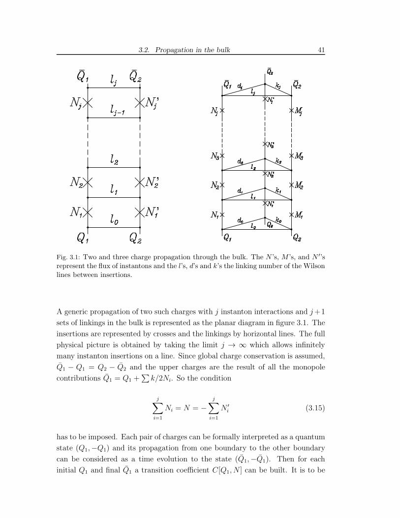
3.2. Propagation in the bulk 41
Fig. 3.1: Two and three charge propagation through the bulk. The N ’s, M ’s, and N ′’srepresent the flux of instantons and the l’s, d’s and k’s the linking number of the Wilsonlines between insertions.
A generic propagation of two such charges with j instanton interactions and j+1
sets of linkings in the bulk is represented as the planar diagram in figure 3.1. The
insertions are represented by crosses and the linkings by horizontal lines. The full
physical picture is obtained by taking the limit j → ∞ which allows infinitely
many instanton insertions on a line. Since global charge conservation is assumed,
Q1 − Q1 = Q2 − Q2 and the upper charges are the result of all the monopole
contributions Q1 = Q1 +∑
k/2Ni. So the condition
j∑
i=1
Ni = N = −j∑
i=1
N ′i (3.15)
has to be imposed. Each pair of charges can be formally interpreted as a quantum
state (Q1,−Q1) and its propagation from one boundary to the other boundary
can be considered as a time evolution to the state (Q1,−Q1). Then for each
initial Q1 and final Q1 a transition coefficient C[Q1, N ] can be built. It is to be

42 3. Toroidal Compactification Spectrum and the Heterotic String
interpreted as the square root of a probability exactly as in a quantum system.
(Q1,−Q1) → C[Q1, N ] (Q1 +k
2N,−Q1 −
k
2N) (3.16)
where condition (3.15) was already used.
C is a function of Q1 and N only but, in order to find it, it is necessary to take into
account all the possible processes in the bulk, monopole interactions and linkings.
To be able to extract some information about the boundary let us insert a new
variable l, which denotes the total linking number. Up to a normalization factor,
C can be written as
C[Q1, N ] =
∞∑
l=−∞
∫
dl δ(l − l) c[Q1, N, l] (3.17)
with the definition
l = l0 +
j∑
i=1
li (3.18)
It is now time to determine how the infinitely many bulk processes contribute
to this coefficient. Due to the interaction with the monopoles labeled by i, the
pair of charges will go through the transition (q, q′) → (q + k/2Ni, q′ + k/2N ′
i)
according to (2.24). Between each monopole insertion the linking will induce a
phase change of 4πiqq′li/k according to (2.25). The total change of the charges
is already taken into account through the N dependence of C. But the processes
that are being summed over must be selected in order to fulfill the requirement
that the total monopole contribution is N and that the total linking number is
l. The coefficient c is then the sum of the phases
c[Q1, N, l] =∑
Na,N ′
b
∑
li,l0
exp2πiΦ[Na, N′b, li, l0] (3.19)
where the sums over Na and N ′b stand for all the allowed configurations obeying
(3.15) and the sum over li and l0 for the ones obeying (3.18). The phase, Φ, for
each process is simply the sum of the several phases induced at each step i along

3.2. Propagation in the bulk 43
the propagation in the bulk (see figure 3.1)
Φ =2
k
−Q21l0 +
j∑
i=1
(
Q1 +k
2
i∑
b=1
Nb
)(
−Q1 +k
2
i∑
a=1
N ′a
)
li
(3.20)
Writing the last term of the sum in i by using (3.15), i.e. for i = j, and expanding
the products, are obtain
Φ =2
k
−Q21 l0 −Q2
1
j∑
i=1
li +
(
Q21 −
(
Q1 +k
2N
)2)
lj
+k
2
j−1∑
i=1
(
Q1
i∑
a=1
(N ′a −Na) +
k
2
i∑
a=1
N ′a
i∑
b=1
Nb
)
li
(3.21)
Note that the phase is no longer Nj dependent, as it was replaced by the N depen-
dence. Furthermore it is necessary to get the l dependence of c. In the following
discussion it is investigated in which cases this coefficient is non vanishing.
Bearing in mind that these coefficients are actually formal series (which are diver-
gent in general), different ways of factorizing the sums is safer. So three different
factorizations will be considered below (it is argued that these are the only possi-
ble factorizations). c will factorize into an l dependent phase and one independent
of l. Unless otherwise stated, from now on, the index i will run from 1 to j − 1.
The most obvious way to factorize the sum is to eliminate l0 = l−∑ li− lj . Then(3.19) factorizes as
c[Q1, N, l] = exp
−2πi2
kQ2
1 l
×
×∞∑
Na=−∞
∞∑
N ′
b=−∞
j−1∏
i=1
∞∑
li=−∞
∞∑
lj=−∞
exp2πiΦ′0[Na, Nb, li, lj]
(3.22)
The indices a and b run from 1 to j− 1. Since the phase Φ′0 is the sum of several
44 3. Toroidal Compactification Spectrum and the Heterotic String
phase changes φ, the second factor can be rewritten as
∑
Na,N ′
b
(
j−1∏
i=1
∞∑
li=−∞
exp2πiφi li)
∞∑
lj=−∞
exp2πiφj lj
(3.23)
where
φi = Q1
i∑
a=1
(N ′a −Na) +
k
2
i∑
a=1
N ′a
i∑
b=1
Nb
φj =2
k
Q21 −
(
Q1 +k
2N
)2
(3.24)
Now each of the sums over lj and the li’s can be considered independently. If
one of them is zero c will be vanishing. Note that although normalization factors
have not been discussed here, each of these phase sums must be normalized to a
number between 0 and 1 such that C2 is interpreted as a probability, because C
is the coefficient of a quantum state. Further, if one takes the limit of j → ∞these sums will become integrals. It can be investigated if they are zero or not
by using the identity
∞∑
q=−∞exp2πi φ q =
∞∑
p=−∞δ(φ− p) (3.25)
The sum over delta functions is zero if φ is not an integer. The conclusion is then
that, for every i, φi must be an integer. Summing over lj the restriction
2
k
Q21 −
(
Q1 +k
2N
)2
∈ Z (3.26)
is obtained. Replacing Q1 by its form (2.23), expanding and getting rid of the
even integer term 2mN which does not change anything concerning the condition
being imposed, the former condition reads
k
2N (n+N) ∈ Z (3.27)

3.2. Propagation in the bulk 45
For irrational k the only two solutions are
N = 0 (3.28)
N = −n (3.29)
The physical meaning of these results will be given a little later. The remaining
conditions on the φi’s will allow us to build the intermediate processes, which
will be addressed at the end of this section.
An other way to carry out the sums is to eliminate lj = l− l0−∑
li. Then (3.19)
factorizes as
c[Q1, N, l] = exp
−2πi2
k
(
Q1 +k
2N
)2
l
×
×∞∑
Na=−∞
∞∑
N ′
b=−∞
j−1∏
i=1
∞∑
li=−∞
∞∑
l0=−∞
exp2πiΦ′j[Na, Nb, li, l0]
(3.30)
where the phase is now
Φ′j =
2
k
−(
Q21 −
(
Q1 +k
2N
)2)
l0
+k
2
j−1∑
i=1
[
Q1
(
i∑
a=1
(N ′a −Na) + 2N
)
+k
2
(
i∑
a=1
N ′a
i∑
b=1
Nb +N2
)]
li
(3.31)
By performing the sum over l0 the same conditions (3.26) and (3.27) on N are
obtained. There are extra 2N and N2 factors but they do not change the coeffi-
cient c. This can be checked explicitly by replacing Q1 by its form (2.23). Apart
from an irrelevant factor of 4πimN one gets the same result as for Φ′0.
A third factorization is studied next. Rewriting (3.21) in terms of l± defined by
l+0 = l0 + lj l−0 = l0 − lj (3.32)

46 3. Toroidal Compactification Spectrum and the Heterotic String
and taking into account that l+0 = l −∑ li, (3.19) factorizes as
c[Q1, N, l] = exp
−2πi2
k
(
Q21 +
(
Q1 +k
2N
)2)
l
2
×
×∞∑
Na=−∞
∞∑
N ′
b=−∞
∞∑
li=−∞
∞∑
l−0=−∞
exp2πiΦ′+[Na, Nb, li, l
−0 ]
(3.33)
The new phase is
Φ′+ =
2
k
−(
Q21 −
(
Q1 +k
2N
)2)
l−02
+k
2
j−1∑
i=1
[
Q1
(
i∑
a=1
(N ′a −Na) +N
)
+k
2
(
i∑
a=1
N ′a
i∑
b=1
Nb +1
2N2
)]
li
(3.34)
By performing the sum over l−0 a new different condition is obtained
2
k
Q21 −
(
Q1 +k
2N
)2
∈ 2Z (3.35)
By expanding Q1 this is simply
k
2N (n+N) ∈ 2Z (3.36)
For generic k ∈ R the same solutions as in (3.26) are obtained and apparently
this condition turns out to hold the same results of (3.27). It will become clear
that this last result is different from the previous two cases. As before the extra
N and N2/2 factors do not change the coefficient.
It is now time to explain the physical implications of the three previous results.
The phase factors in front of l are none other than the conformal dimensions (2.27)
of the vertex operators inserted on the boundary CFT’s. When the sum over l0
was eliminated it gave (3.22). Extracting the l phase factor gives
2
kQ2
1 = 2∆ = ∆1 +∆2 (3.37)

3.2. Propagation in the bulk 47
Upon elimination of the lj sum the factorization (3.30) was obtained such that
the phase factor reads2
kQ2
1 = 2∆ = ∆1 + ∆2 (3.38)
while for the factorization (3.33), where the sum over l+0 was eliminated, we
obtained1
k(Q2
1 + Q21) = ∆ + ∆ (3.39)
Note that no other factors can be extracted. Trying to eliminate any other com-
bination of l0 and lj would yield the result c = 0. Eliminating some combination
of li’s will always end up effectively in extracting one of the three above factors or,
again, give the result c = 0. The solutions for the monopole interactions (3.45)
and (3.47) computed below assure this result.
In order for C not to be zero it is necessary to get integer conformal dimensions
as stated in section 3.1. Consider then adding extra type B gauge fields. One
Wilson line (3.4) carries now charges from all the U(1)’s. Summing over l for the
three previous cases the conditions
r = 2
(
∆+p2
k′
)
∈ Z
s = 2
(
∆ +p2
k′
)
∈ Z
t = ∆+ ∆ +2p2
k′∈ Z
(3.40)
are obtained. Subtracting the second equation from the first gives the equation
r − s = 2(∆− ∆) =2
k(Q2
1 − Q21) = −2mN (3.41)
where N = 0,−n according to the allowed solutions (3.28) and (3.29). By averag-
ing the first two conditions, the third one is obtained as long as the identification
t = (r + s)/2 (3.42)
is considered. According to the discussion in section 3.1 r and s have to be even

48 3. Toroidal Compactification Spectrum and the Heterotic String
in order for the full conformal dimension to be integer. Making the identifications
r
2= 1− L
s
2= 1− L
(3.43)
the mass shell condition (3.7) is retrieved. Furthermore, (3.41) becomes the spin
condition (3.8).
Below the possible intermediate processes are investigated by performing the
sums over each of the li’s. Remembering that the total charge at each level is
null, a chain of conditions φi ∈ Z is obtained. These conditions allow the building
of the full set of possible diagrams contributing to the transitions. Starting with
i = 1 a simple condition is found
n(N ′1 −N1) + 2N1N
′1 = 0 (3.44)
It has two possible solutions
a N1 = 0 = N ′1
b N1 = −n = −N ′1
(3.45)
For i = 2 the condition reads
n(N ′1 −N1) + n(N ′
2 −N2) + 2N1N′1 + 2N2N
′2 + 2N1N
′2 + 2N2N
′1 = 0 (3.46)
Choosing a for N1 and N ′1 the same two previous solutions for N2 and N ′
2 are
obtained. Choosing the b solution for N1 and N ′1, again two solutions are valid
for N2 and N ′2: a or a new solution
b N2 = n = −N ′2 (3.47)
If this solution is chosen for i = 2, an a or b solution will be allowed for i = 3.
So no new solutions emerge and the solution for generic i can be built using the
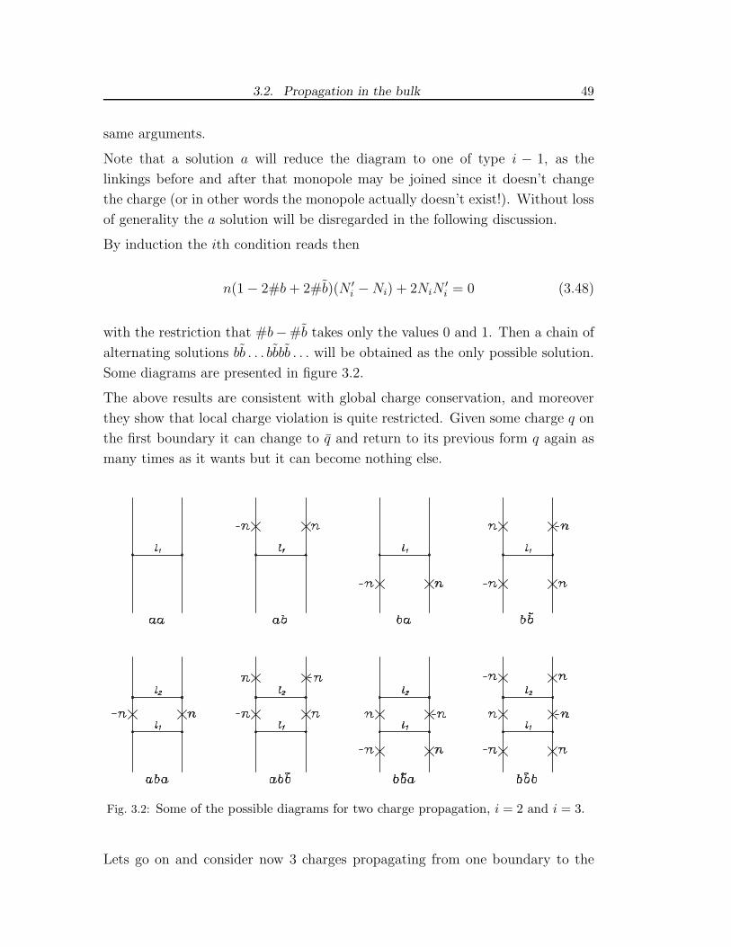
3.2. Propagation in the bulk 49
same arguments.
Note that a solution a will reduce the diagram to one of type i − 1, as the
linkings before and after that monopole may be joined since it doesn’t change
the charge (or in other words the monopole actually doesn’t exist!). Without loss
of generality the a solution will be disregarded in the following discussion.
By induction the ith condition reads then
n(1− 2#b+ 2#b)(N ′i −Ni) + 2NiN
′i = 0 (3.48)
with the restriction that #b−#b takes only the values 0 and 1. Then a chain of
alternating solutions bb . . . bbbb . . . will be obtained as the only possible solution.
Some diagrams are presented in figure 3.2.
The above results are consistent with global charge conservation, and moreover
they show that local charge violation is quite restricted. Given some charge q on
the first boundary it can change to q and return to its previous form q again as
many times as it wants but it can become nothing else.
Fig. 3.2: Some of the possible diagrams for two charge propagation, i = 2 and i = 3.
Lets go on and consider now 3 charges propagating from one boundary to the

50 3. Toroidal Compactification Spectrum and the Heterotic String
other (or equivalently evolving in time)
Q1 → Q1
Q2 → Q2
Q3 = −Q1 −Q2 → Q3 = −Q1 − Q2
(3.49)
as pictured in figure 3.1. The phase is now
Φ3 =2
k
Q1Q2l0 −Q2(Q1 +Q2)d0 −Q1(Q1 +Q2)k0+
+
j−1∑
i=1
[
Q21(i)li − Q1(i)Q3(i)di − Q2(i)Q3(i)ki
]
+ Q1Q2lj − Q2(Q1 + Q2)dj − Q1(Q1 + Q2)kj
(3.50)
where the following definitions
Q1(i) = Q1 +k
2
i∑
a=1
Ni Q1 = Q1 +k
2N
Q2(i) = Q2 +k
2
i∑
a=1
Mi Q2 = Q2 +k
2M
Q3(i) = Q1 +Q2 −k
2
i∑
a=1
N ′i Q3 = Q1 +Q2 −
k
2N ′
(3.51)
were used. Now it can be chosen to factor out some combination of l0, d0, k0,
lj , dj and kj. But it is now clear, from the previous discussion of two charge
propagation, what factorizations one should look for. So the sensitive choices are
to eliminate all the 0’s, all the j’s or some particular combination of 0’s and j’s
for the three linkings.
The dependence on l0, d0 and k0 in the sums can be replaced by sums over the
total linking numbers defined as l = l0 +∑
li + lj, d = d0 +∑
di + dj and
k = k0 +∑
ki + kj. Then the phases (conformal dimensions) appearing in the
three field correlation functions given in (2.29) for z12, z23 and z13 correspond to

3.2. Propagation in the bulk 51
the phase factors containing l, d and k respectively.
By considering extra type B gauge fields with charges p1, p2 and p3 and summing
over the previous variables gives the conditions that the combinations of confor-
mal dimensions in (2.29) must be integer. The conformal dimensions are to be
read off by considering these extra gauge fields and charges ∆ = Q2/k + p2/k′
and ∆ = Q2/k + p2/k′. From now on let us use this definition of conformal
dimensions. As discussed in section 3.1, from the point of view of the boundary
CFT’s, these factors must indeed be integer to ensure that the three point OPE’s
are single valued.
In terms of the individual vertices it is not so clear what these conditions mean.
Without loss of generality and in order to clarify them let us replace the sums
over l, d and k by the sums over three new variables l+, d+ and k+ such that
l = l+ + k+, d = d+ + l+ and k = k+ + d+. By summing over these new variables
one obtains the following conditions
2∆1, 2∆2, 2∆3 ∈ Z (3.52)
In a similar way the dependence over lj, dj and kj can be replaced by a dependence
over l+, d+ and k+ and, upon summation, the respective conditions are obtained
2∆1, 2∆2, 2∆3 ∈ Z (3.53)
Or using the definition (3.32) for l±0 , d±0 and k±0 and replacing the l+0 , d
+0 and k+0
dependences by l+, d+ and k+ in the same way as before (performing the sums
in these last variables) we get the conditions
∆1 + ∆1, ∆2 + ∆2, ∆3 + ∆3 ∈ Z (3.54)
Similarly to the previous discussion for two charge propagation these conditions
turn out to be equivalent to the mass shell and spin conditions of string theory.
The fundamental differences come from the remaining conditions. By taking
the first two cases (3.52) and (3.53), where the 0’s and j’s linking number sum
dependences were replaced, and summing over (l+j, d+j, k+j) and (l+0, d+0, k+0)
gives, in both cases, three conditions. The first two are redundant, as they
correspond to (3.26) which has been obtained from the two charge propagation,

52 3. Toroidal Compactification Spectrum and the Heterotic String
while the third one is new
4
k
(
Q1Q2 − Q1Q2
)
∈ Z (3.55)
Nevertheless the solutions for irrational k end up being of the same kind as before.
There are two solutions
N = 0
M = 0
N = −n1
M = −n2
(3.56)
For the case of (3.54), where the sum over +’s linking number was replaced, one
finds, upon summation over (l−+0, d−+0, k
−+0), the two conditions (3.35) which were
obtained in the two charge case. The third one is again new
2
k
(
Q1Q2 − Q1Q2
)
∈ Z (3.57)
The solutions for the full diagrams are very similar to the ones of two charges,
with the charges oscillating simultaneously between Q1, Q2 and Q1 = Q1−n1k/2,
Q2 = Q2 − n2k/2. For four charges there are no new conditions.
After all this algebra let us summarize what was obtained so far. In the start
there was a theory which, at the perturbative level, had the allowed charges of the
form Q = m+ (k/4)n. It was shown that, under certain assumptions, if the non-
perturbative processes are taken into account, the charge spectrum is modified
(restricted) quite drastically. The allowed left/right pair of charges are in one-
to-one correspondence with the processes which have non vanishing quantum
amplitudes. All these processes can be organized in a lattice Γ with elements
l = (Q, Q = Q + (k/2)N) with N either 0 or −n. Moreover a Lorentzian inner
product of signature (+,−) emerges naturally from (3.26), (3.35) and (3.57)
defined by
l l′ = 2
k(QQ′ − QQ′) (3.58)
There is more to add to it, going even further and extracting very important

3.3. Boundary conditions 53
properties of the lattice, it is even due to (3.35)
l l = 2
k(Q2 − Q2) ∈ 2Z (3.59)
and integer due to (3.57)
l l′ = 2
k(QQ′ − QQ′) ∈ Z (3.60)
Note that (3.55) is redundant since it is necessarily obeyed if (3.57) is.
By inspection, forN = −n the lattice is self-dual as well but not forN = 0. Note
that the dual lattice Γ∗ is defined as the set of all points in R1,1 (or Rd,d generally)
which have integer inner product with all the points in the original lattice Γ. In
this way the condition of the lattice being integer is only the statement that
Γ ⊂ Γ∗.
In the next section it will be explained how to exclude the N = 0 case and obtain
what is sought. The lattice is then exactly the one for bosonic string theory with
one compact dimension. It is the Narain lattice for compactification on S1. For
toroidal compactification of several dimensions it is enough to consider several
compact gauge fields. This situation is described in section 3.5.
3.3 Boundary conditions
So it remains to understand what mechanism selects between the N = 0 and
N = −n cases. The key is to consider different combinations of the boundary
conditions introduced in (2.7). Furthermore, to obtain a CFT on the boundary
(whether it is chiral or not) as an effective 2D theory of the 3D TMGT, it is
necessary to identify the two boundaries Σ0 and Σ1 in some way. These are the
mechanisms that allow us to build several string theories out of the same 3D
theory. Note that these constructions are only possible due to the Maxwell term
in the action and the existence of monopoles.
In the last section it was shown that the bulk theory only allows the charge
q = m+ kn/4 to become q = m− kn/4 or remain unchanged. What is actually
n? Going back to (2.23), 2πn is the flux of the magnetic field. So upon some
kind of boundary identification the theory only admits the ones that support one

54 3. Toroidal Compactification Spectrum and the Heterotic String
of the conditions
N = 0
∫
Σ0
d2z0B =
∫
Σ1
d2z1B
N = −n∫
Σ0
d2z0B = −∫
Σ1
d2z1B
(3.61)
Consider a map (coordinate transformation) that transforms a vector in Σ1 into
another vector in Σ0, defining in this way the identification rule. There will
be two kinds of maps. One which maintains the relative orientation of both
2D boundaries, let us call it parallel (//), and one that reverses the relative
orientation, let us call it perpendicular (⊥). The names are chosen by the relative
identification of the axes from boundary to boundary as pictured in figure 3.3.
Note that the induced ǫ does not change from boundary to boundary. From
the 3D point of view time is being reversed on one boundary and the complex
coordinates are swapped (in 3D this is a rotation). From the point of view of the
bulk nothing special is happening.
Fig. 3.3: Boundary identification with the same orientation (parallel; //) and reversedorientation (perpendicular; ⊥)
Let the difference of fluxes be defined as
δφ =
∫
Σ1
d2z1B −∫
Σ0
d2z0B =
∫
Σ1
d2zǫij∂iAj −∫
Σ0
d2zǫij∂iAj (3.62)
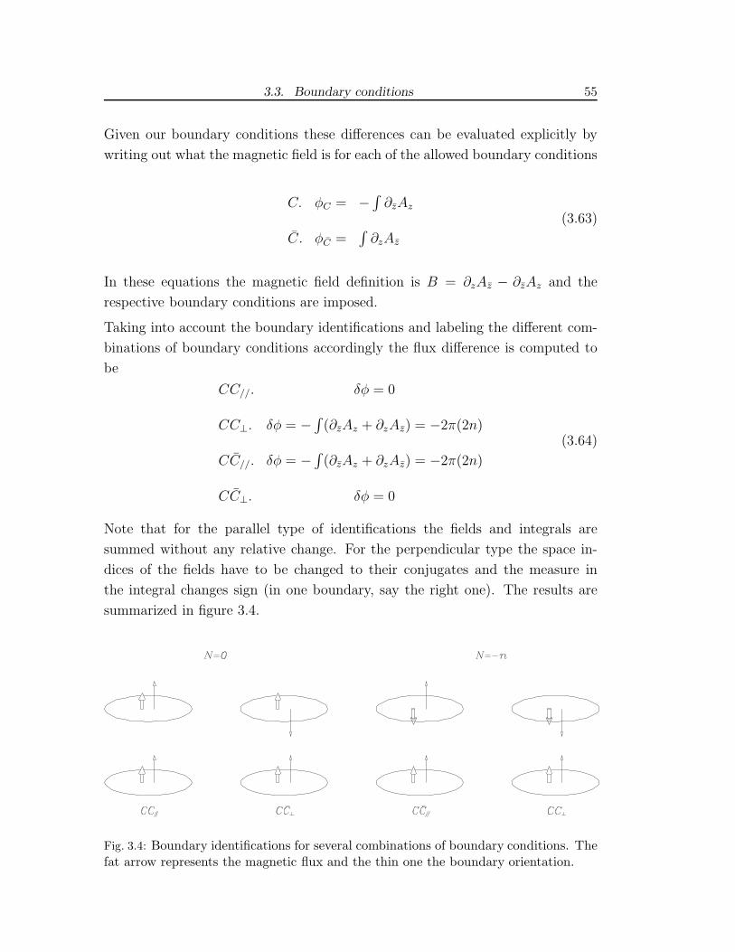
3.3. Boundary conditions 55
Given our boundary conditions these differences can be evaluated explicitly by
writing out what the magnetic field is for each of the allowed boundary conditions
C. φC = −∫
∂zAz
C. φC =∫
∂zAz
(3.63)
In these equations the magnetic field definition is B = ∂zAz − ∂zAz and the
respective boundary conditions are imposed.
Taking into account the boundary identifications and labeling the different com-
binations of boundary conditions accordingly the flux difference is computed to
be
CC//. δφ = 0
CC⊥. δφ = −∫
(∂zAz + ∂zAz) = −2π(2n)
CC//. δφ = −∫
(∂zAz + ∂zAz) = −2π(2n)
CC⊥. δφ = 0
(3.64)
Note that for the parallel type of identifications the fields and integrals are
summed without any relative change. For the perpendicular type the space in-
dices of the fields have to be changed to their conjugates and the measure in
the integral changes sign (in one boundary, say the right one). The results are
summarized in figure 3.4.
Fig. 3.4: Boundary identifications for several combinations of boundary conditions. Thefat arrow represents the magnetic flux and the thin one the boundary orientation.

56 3. Toroidal Compactification Spectrum and the Heterotic String
So the conclusion is that Q = Q corresponds to CC//, CC//, CC⊥ or CC⊥ and
Q − Q = (k/2)n to CC⊥, CC⊥, CC// or CC// boundary conditions. Note that
in principle there may exist other choices of the maps which would give different
boundary theories.
Note that the spectrum for NC or NC boundary conditions must be obtained
by truncating the spectrum of CC⊥ or CC//. Simply consider the charge on the
N boundary to be restricted to Q = 0. This means
m =k
4n (3.65)
Then the charges on the other boundary become
Q =k
2n (3.66)
Of course for irrational k the only solution for the condition (3.65) is m = n = 0
and a very poor and empty theory is obtained in the boundary. In section 3.5
it will be clarified in which cases the condition (3.65) allows some dynamics on
the boundary. Trying to truncate the spectrum of CC// or CC⊥ will set straight
away Q = Q = 0 since the charges are equal on both boundaries killing the hope
of finding any dynamics on the boundaries.
From now on it is chosen to work with CC⊥ or CC// type of boundary conditions
by default since they are the ones which give us the desired spectrum on the
boundary CFT’s. Furthermore, as just explained, N boundary conditions can
easily be obtained from them.
3.4 RCFT’s and Fusion Rules
In section 3.1 a short overview on RCFT and fusion rules was given. In what
follows it will be explained how the fusion rules and the RCFT block structure
emerge, with some naturalness, from the bulk theory. Take k = 2p/q to be a
rational number. Note that in the previous discussion 2p′ = p, so take even
p. By inspection it can be checked that the (m,n) space is divided in diagonal
bricks containing p× q charges. They are distributed in diagonal layers of identi-
cally valued bricks as symbolically pictured in figure 3.5. To build this diagonal
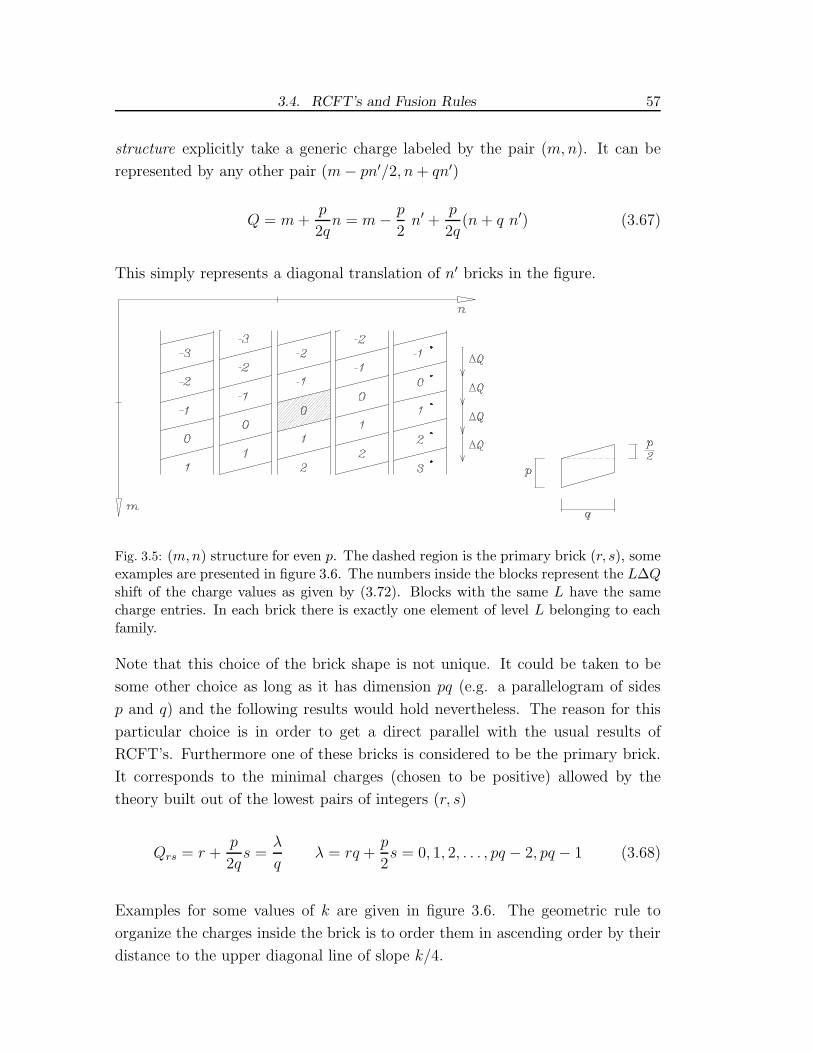
3.4. RCFT’s and Fusion Rules 57
structure explicitly take a generic charge labeled by the pair (m,n). It can be
represented by any other pair (m− pn′/2, n+ qn′)
Q = m+p
2qn = m− p
2n′ +
p
2q(n+ q n′) (3.67)
This simply represents a diagonal translation of n′ bricks in the figure.
Fig. 3.5: (m,n) structure for even p. The dashed region is the primary brick (r, s), someexamples are presented in figure 3.6. The numbers inside the blocks represent the L∆Qshift of the charge values as given by (3.72). Blocks with the same L have the samecharge entries. In each brick there is exactly one element of level L belonging to eachfamily.
Note that this choice of the brick shape is not unique. It could be taken to be
some other choice as long as it has dimension pq (e.g. a parallelogram of sides
p and q) and the following results would hold nevertheless. The reason for this
particular choice is in order to get a direct parallel with the usual results of
RCFT’s. Furthermore one of these bricks is considered to be the primary brick.
It corresponds to the minimal charges (chosen to be positive) allowed by the
theory built out of the lowest pairs of integers (r, s)
Qrs = r +p
2qs =
λ
qλ = rq +
p
2s = 0, 1, 2, . . . , pq − 2, pq − 1 (3.68)
Examples for some values of k are given in figure 3.6. The geometric rule to
organize the charges inside the brick is to order them in ascending order by their
distance to the upper diagonal line of slope k/4.
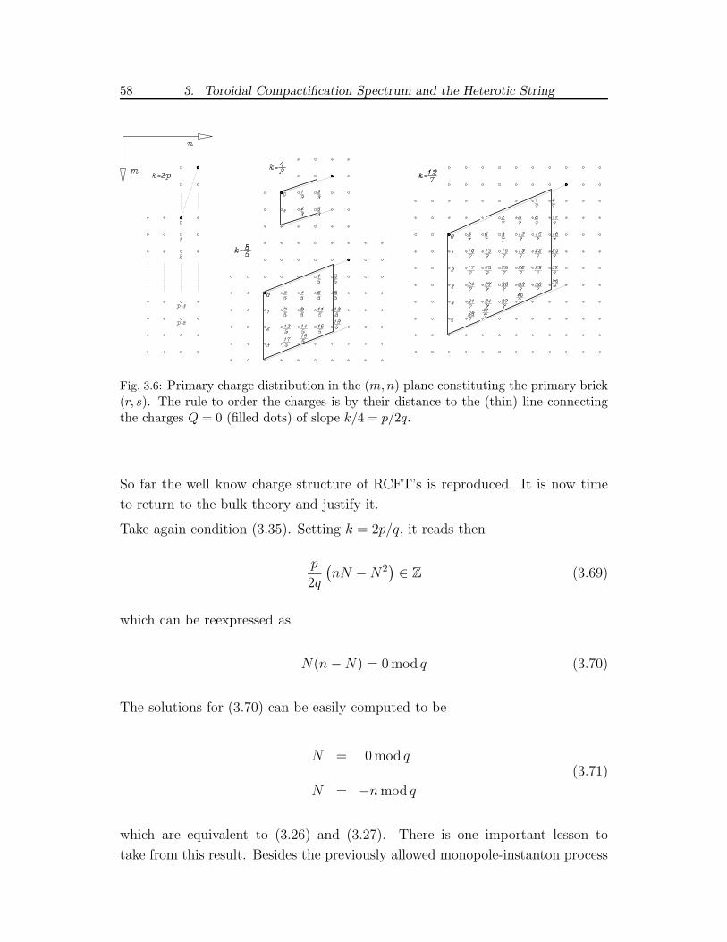
58 3. Toroidal Compactification Spectrum and the Heterotic String
Fig. 3.6: Primary charge distribution in the (m,n) plane constituting the primary brick(r, s). The rule to order the charges is by their distance to the (thin) line connectingthe charges Q = 0 (filled dots) of slope k/4 = p/2q.
So far the well know charge structure of RCFT’s is reproduced. It is now time
to return to the bulk theory and justify it.
Take again condition (3.35). Setting k = 2p/q, it reads then
p
2q
(
nN −N2)
∈ Z (3.69)
which can be reexpressed as
N(n−N) = 0mod q (3.70)
The solutions for (3.70) can be easily computed to be
N = 0mod q
N = −nmod q
(3.71)
which are equivalent to (3.26) and (3.27). There is one important lesson to
take from this result. Besides the previously allowed monopole-instanton process

3.4. RCFT’s and Fusion Rules 59
n→ −n which is charge dependent, there is a new charge independent one:
∆Q = ±p (3.72)
This is actually the physical process that spans each of the families! Or in other
words, the process that builds up each of the conformal blocks of the theory. To
obtain the charges of some family in terms of m and n from the primary one,
either n or m can be shifted as m→ m+ pL or n→ n+ 2qL. This is due to an
infinite degeneracy in the (m,n) plane of the charge values expressed by (3.67).
Figure 3.7 presents the distribution of charges for k = 2p. In this simplified case
the families are simply organized along the m axis for even values of 2n. This
structure is repeated by shifts on the m axis of magnitude p.
Fig. 3.7: Charge structure for k = 2p. Only even values are considered on the n axis
For odd p all the structure is similar but with bricks of dimension p× 2q. Take
again a generic charge Q
Q =p n
2q+m =
p (n+ 2q n′)
2q+m− p n′ (3.73)
Because p is odd, equal-valued charges correspond to pairs related by (m,n) →(m− pn′, n+ 2qn′). The slope of the brick is the same k/4 but they are twice as
large in the n direction. Everything else works in the same way.

60 3. Toroidal Compactification Spectrum and the Heterotic String
3.5 Lattices and The Heterotic String
Consider now an U(1)D action of the type (1.4) with gauge fields obeying Bboundary conditions (replacing k by a generic matrix KIJ) with action
S =
∫
M
d2z dt
[
−√−g(3)4γ
F µνI F I
µν +GIJ +BIJ
8πǫµνλAI
µ∂νAJλ
]
(3.74)
GIJ and BIJ stand for the symmetric and antisymmetric parts of KIJ .
Using the same procedure outlined in section 2.1 the effect of monopole-instantons
is computed to induce a change of the charge
∆QI =GIJ
2NJ (3.75)
Using the Schrodinger picture the charge spectrum is computed to be
QI = mI +KIJ
4nJ (3.76)
Note that the antisymmetric part BIJ is present in the charge but not in the
monopole effects. This is due to the fact that it is manifested only at the level
of the boundary. Also in the action the term corresponding to BIJ is a total
derivative and can be completely integrated out to the boundary
∫
M
BIJǫµνλAI
µ∂νAJλ =
1
2
[
−∫
Σ0
BIJ ǫijAI
iAJj +
∫
Σ1
BIJ ǫijAI
iAJj
]
(3.77)
Let us analyze first the case for BIJ = 0. The previous discussion of section 3.3
follows in the same fashion. Choosing CC⊥ or CC// boundary conditions, the
desired relative spectrum in each boundary is obtained, that is, Q = m+Kn/4
and Q = m − Kn/4. This means that every monopole contribution of the
form (3.75) has exactly NJ = −nJ .
What about if BIJ 6= 0? Returning to a more careful analysis of the boundary
identifications, for CC⊥ the measures of the integrals in opposite boundaries
change their relative sign, say∫
1d2z → −
∫
1d2z, due to the 2D measure changing
sign. The fields in one boundary (say Σ1) are swaped, Ai ↔ Aj . Note that neither

3.5. Lattices and The Heterotic String 61
BIJ nor ǫij in the right integral are being changed, they are induced from the
bulk and do not change by these kinds of boundary identifications. Thus this
transformation has no effect in the BIJ term
∫
Σ0
BIJǫijAI
iAJj →
∫
Σ0
BIJǫijAI
iAJj (3.78)
For CC// nothing changes either. This means that the BIJ term does not change
sign under any of our boundary identifications.
So the left/right spectrum obtained is
QI =GIJ +BIJ
4nJ +mI
QI =−GIJ +BIJ
4nJ +mI
(3.79)
such that the charge difference QI − QI = GIJ nJ/2 is indeed the monopole
contribution.
Similarly the lattice obtained is of the form l = (Q, Q) with the Lorentzian
product of signature (+,−) defined as
l l′ = 2G(−1)IJ(QIQ′J − QIQ
′J) (3.80)
where G−1 stands for the inverse of GIJ . The signature of the product has D
plus and D minus signs. The properties of this lattice are the same as the ones
for the previous D = 1 case and follow in a similar way from the bulk theory as
presented in section 3.2. The lattice is integer, even and self-dual.
It is now time to analyze which lattices do exist for CN boundary conditions. As
explained before in section 3.3 they can be obtained by truncating the lattices
where NJ = −nJ . Imposing CN is then equivalent to truncating the lattice
by choosing Q = 0. Similarly to (3.65), this means elements of the lattice are
selected such that
mI =GIJ − BIJ
4nJ (3.81)
This sublattice has elements l = (Q, 0) with Q built out of n and m obey-
ing (3.81). Once Q = 0 the Lorentzian product (3.80) becomes, for this particular
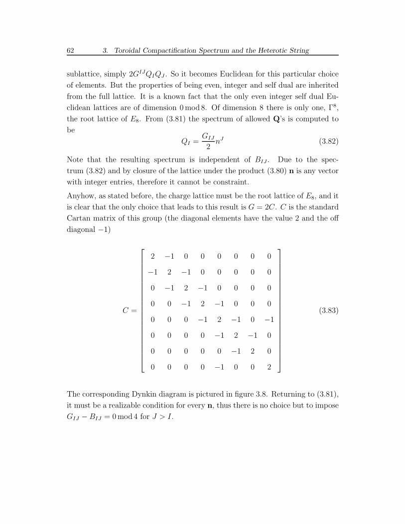
62 3. Toroidal Compactification Spectrum and the Heterotic String
sublattice, simply 2GIJQIQJ . So it becomes Euclidean for this particular choice
of elements. But the properties of being even, integer and self dual are inherited
from the full lattice. It is a known fact that the only even integer self dual Eu-
clidean lattices are of dimension 0mod 8. Of dimension 8 there is only one, Γ8,
the root lattice of E8. From (3.81) the spectrum of allowed Q’s is computed to
be
QI =GIJ
2nJ (3.82)
Note that the resulting spectrum is independent of BIJ . Due to the spec-
trum (3.82) and by closure of the lattice under the product (3.80) n is any vector
with integer entries, therefore it cannot be constraint.
Anyhow, as stated before, the charge lattice must be the root lattice of E8, and it
is clear that the only choice that leads to this result is G = 2C. C is the standard
Cartan matrix of this group (the diagonal elements have the value 2 and the off
diagonal −1)
C =
2 −1 0 0 0 0 0 0
−1 2 −1 0 0 0 0 0
0 −1 2 −1 0 0 0 0
0 0 −1 2 −1 0 0 0
0 0 0 −1 2 −1 0 −1
0 0 0 0 −1 2 −1 0
0 0 0 0 0 −1 2 0
0 0 0 0 −1 0 0 2
(3.83)
The corresponding Dynkin diagram is pictured in figure 3.8. Returning to (3.81),
it must be a realizable condition for every n, thus there is no choice but to impose
GIJ −BIJ = 0mod 4 for J > I.

3.5. Lattices and The Heterotic String 63
The only possibilities left are
GIJ = 2CIJ
BIJ = (2 + 4r)CIJ J > I, r ∈ Z
(3.84)
Fig. 3.8: Dynkin Diagram of E8
There are two lattices of dimension 16 obeying these properties: Γ8 × Γ8 with
elements in the root lattice of E8 ×E8 and Γ16. The well known results of string
theory are retrieved. Note that in the first works of the non-interacting Heterotic
string [48] there is no mention of the tensor BIJ (the free spectrum depends solely
on GIJ). Only after the introduction of interactions and an effective action for
the theory [49] does it becomes clear that there is a need for BIJ . For r = 0 the
result presented in [60] and references therein is obtained up to the normalization
of 1/4 on KIJ .

64 3. Toroidal Compactification Spectrum and the Heterotic String
4. OPEN AND UNORIENTED STRINGS
This Chapter is based on the original work of the author and Ian Kogan [35].
Although originally (and historically) open string theories were considered as
theories by themselves, it soon become evident that, whenever they are present,
they come along with closed (non-chiral) strings. Moreover open string theories
are obtained from closed string theories by gauging certain discrete symmetries
of the closed theory (see [66] and references therein for a discussion of this topic).
The way to get open strings from closed strings is by gauging the world-sheet
parity [66–68], Ω : z → −z. That is, the identification σ1 ∼= −σ1 is imposed,
where z = σ1 + iσ2 and z = σ1 − iσ2 is the complex structure of the world-sheet
manifold. The spaces obtained in this way can be of two types: closed unoriented
and open oriented (and unoriented as well). These last ones are generally called
orbifolds and the singular points of the construction become boundaries. The
states (operators and fields of the theory in general) of the open/unoriented theory
are obtained from the closed oriented theory by projecting out the ones which
have negative eigenvalues of the parity operator. This is obtained by building
a suitable projection operator (1 + Ω)/2 such that only the states of positive
eigenvalue are kept in the theory. Namely the identification XI(z, z) ∼= XI(z, z)
or XIL(z)
∼= XIR(z) (in terms of the holomorphic and antiholomorphic parts of
X = XL +XR) holds.
Another construction in string theory is orbifolding the target space of the theory
under an involution of some symmetry of that space. In this work only a Z2
involution is going to be considered, imposing the identificationXI ∼= −XI , where
XI are the target space coordinates. When combining both constructions, world-
sheet and target space orbifolding, open/unoriented theories on orbifolds [69–72]
or orientifolds (XI(z, z) = −XI(z, z)) are obtained, implying the existence of
twisted sectors in the open/unoriented theories.
Further to the previous discussion both sectors (twisted and untwisted) need
to be present for each surface in order to ensure modular invariance of the full
66 4. Open and Unoriented Strings
partition function [66,73,83]. One point that must be stressed is that twisting in
open strings can, for the case of a Z2 target space orbifold, be simply interpreted
as the choice of boundary conditions: Neumann or Dirichlet.
Toroidal compactification is an important construction in string theories and
in the web of target space dualities. Early works considered also open string
constructions in these toroidal backgrounds [73, 74]. In these cases some target
space coordinates are compactified, say XJ(z + 2πi, z − 2πi) ∼= XJ(z, z) + 2πR
(R is the radius of compactification of XJ), and the twisted states in the theory
are the ones corresponding to the points identified under XJ(z + 2πi, z − 2πi) ∼=−XJ(z, z) + 2πR, or in terms of the holomorphic and antiholomorphic parts of
X , XIL(z)
∼= −XIR(z).
An important result coming from these constructions is that the gauge group of
the open theory, the Chan-Paton degrees of freedom carried by the target space
photon Wilson lines (only present in open theories), is constrained, due both
to dualities of open string theory [73] and to modular invariance of open and
unoriented theories [73–76]. This will result in the choice of the correct gauge
group that cancels the anomalies in the theory.
One fundamental ingredient of string theory is modular invariance. Although
for bosonic string theory the constraints coming from genus 1 amplitudes are
enough to ensure modular invariance at generic genus g, it becomes clear that
once the fermionic sector of superstring theory is considered it is necessary to
consider genus 2 amplitude constraints. For closed strings (types II and 0) the
modular group at genus g is PSL(2g,Z) and the constraints imposed by modular
invariance at g = 2 induce several possible projections in the state space of the
theory [77–81] such that the resulting string theories are consistent. Among them
are the well known GSO projections [82] that insure the correct spin-statistics
connection, project out the tachyon and ensure a supersymmetric effective theory
in the 10D target space.
Once an open superstring theory (type I) is created by orbifolding the world-sheet
parities, for each open (and/or unoriented) surface a Relative Modular Group still
survives the orbifold at each genus g [83]. Again in a similar way to the closed
theory the modular invariance under these groups will result in generalized GSO
projections [83–86].
For a more recent overview of the previous topics see [87,88] (see also [42] for an
extensive explanation of them).

67
The purpose of this Chapter is to build open, open unoriented, and closed unori-
ented string theories (with and without orbifolding of the target space) from the
Topological Membrane.
Closed string theories are obtained as the effective boundary theory, their world-
sheet is the closed boundary ∂M . Obtaining open string theory raises a problem
because it is necessary to have an open world-sheet to define them. But the
boundary of a boundary is null, ∂∂M = ∅. So naively it seems that TM cannot
describe open strings since world-sheets are already a boundary of a 3D manifold.
The way out is to consider orbifolding of the bulk theory. In this way the fixed
points of the orbifold play the role of the boundary of the 2D boundary of the
3D membrane. This proposal was first introduced by Horava [89] in the context
of pure Chern-Simons theories. His results are going to be extended to TMGT
and the orbifold group reinterpreted as the discrete symmetries of the full gauge
theory.
Other works have developed Horava’s idea. For a recent study on WZWN orbifold
constructions see [90] (and references therein) For an extensive study, although in
a more formal way than our work, of generic Rational Conformal Field Theories
(RCFT) with boundaries from pure 3D Chern-Simons theory see [91] (and refer-
ences therein). Nevertheless in these previous works the monopole processes were
not studied. These are crucial for describing the winding modes and T-duality in
compact RCFT from the TM point of view and, therefore, in compactified string
theories.
An orbifold of the Topological Membrane (and Topologically Massive Gauge The-
ory) [TM(GT)] is considered such that one new boundary is created at the orb-
ifold fixed point. To do this the discrete symmetries of the 3D theory are gauged,
namely PT and PCT . Several P ’s are going to be defined as generalized par-
ity operations. C and T are the usual 3D QFT charge conjugation and time
inversion operations (see [14] for a review). The orbifolding of the string target
space corresponds in pure Chern-Simons membrane theory to the quotient of the
gauge group by a Z2 symmetry [9]. As will be shown, in the full TM(GT), the
discrete symmetry which will be crucial in this construction is charge conjugation
C. Besides selecting between twisted and untwisted sectors in closed unoriented
string theory it will also be responsible for setting Neumann and Dirichlet bound-
ary conditions in open string theory. More generic orbifold groups will not be
considered.

68 4. Open and Unoriented Strings
There are two main new ideas introduced here. Firstly the use of all possible
realizations of P , C and T combinations, which constitute discrete symmetries of
the theory, as the orbifold group. Although the mechanism is similar to the one
previously studied by Horava for pure Chern-Simons theory, the presence of the
Maxwell term constrains the possible symmetries to PT and PCT type only. Also
the interpretation of the orbifold group as the discrete symmetries in the quantum
theory is new, as is the interpretation of charge conjugation C which selects
between Neumann and Dirichlet boundary conditions. This symmetry explains
the T-duality of open strings in the TM framework. It is a symmetry of the 3D
bulk which exchanges trivial topological configurations (without monopoles) with
nontrivial topological configurations (with monopoles). In terms of the effective
boundary CFT (string theory) this means exchanging Kaluza-Klein modes (no
monopole effects in the bulk) with winding number (monopole effects in the bulk).
In section 4.1 we introduce the Riemann surfaces of genus 0 (the sphere), and
genus 1 (the torus), and their possible orbifolds under discrete symmetries which
are identified with generalized parities P .
Section 4.2 gives an account of Neumann and Dirichlet boundary conditions in
usual CFT using the Cardy method [51] of relating n point full correlation func-
tions in boundary Conformal Field Theory with 2n chiral correlation functions
in the theory without boundaries.
Then, in section 4.3 a brief overview of the discrete symmetries of 3D QFT is
given. They are used to orbifold TM(GT) and the 3D configurations compatible
with several orbifolds are considered, both at the level of the field configurations
and of the particular charge spectra corresponding to the resulting theories. It
naturally emerges from the 3D membrane that the configurations compatible
with PCT correspond to Neumann boundary conditions (for open strings) and to
untwisted sectors (for closed unoriented). The configurations compatible with PT
correspond to Dirichlet boundary conditions (for open strings) and twisted sectors
(for closed unoriented). The genus 2 constraints are discussed here although a
more detailed treatment is postponed for future work. Further it is shown that
Neumann (untwisted) corresponds to the absence of monopole induced processes
while for Dirichlet (twisted) these processes play a fundamental role. A short
discussion on T-duality shows that it has the same bulk meaning as modular
invariance, in that both of them exchange PT ↔ PCT .

4.1. Riemann Surfaces:from Closed Oriented to Open and Unoriented 69
4.1 Riemann Surfaces:
from Closed Oriented to Open and Unoriented
Any open or unoriented manifold Σu can, in general, be obtained from some
closed orientable manifolds Σ under identification of a Z2 (or at most two Z2)
involution(s)
π : Σ → Σu = Σ/Z2
(x,−x) → x(4.1)
such that each point in Σu has exactly two corresponding points in Σ conjugate in
relation to the Z2 involution(s). The pair (x,−x) in the last equation is symbolic,
where the second element stands for the action of the group Z2, z2(x) = −x,on the manifold. Usually this operation is closely related to parity as will be
explained bellow. Although in this work the perspective adopted is that the
starting point is a full closed oriented theory and the open/unoriented theory is
obtained by orbifolding it, there is the reverse way of explaining things. This
means that any theory defined on an open/unoriented manifold is equivalently
defined on the closed/oriented manifold which doubles (consists of two copies of)
the original open/unoriented.
Let us summarize how to obtain the disk D2 (open orientable) and projective
plane RP2 (closed unorientable) from the sphere S2 and the annulus C2 (open
orientable), and the Mobius Strip (open unorientable) and Klein bottleK2 (closed
unorientable) from the torus T 2.
4.1.1 The Projective Plane and the Disk obtained from the Sphere
For simplicity we work in complex stereographic coordinates (z = x1 + ix2, z =
x1 − ix2) such that the sphere is identified with the full complex plane. The
sphere has no moduli and the Conformal Killing Group (CKG) is PSL(2,C). A
generic element of this group is (a, b, c, d) with the restriction ad− bc = 1. It acts
on a point z as
z′ =az + b
cz + d(4.2)
It has then six real parameters, that is, six generators. Thus the sphere has six
Conformal Killing Vectors (CKV’s). It is necessary to use two coordinate charts

70 4. Open and Unoriented Strings
to cover the full sphere, one including the north pole and the other one including
the south pole. Usually it is enough to analyze the theory defined on the sphere
only for one of the patches but it is necessary to check that the transformation
between the two charts is well defined. In stereographic complex coordinates the
map between the two charts (with coordinates z, z and u, u) is given by z → 1/u
and z → 1/u.
The disk D2 can be obtained from the sphere under the identification
z ∼= z (4.3)
This result is graphically pictured in figure 4.1 and consists in the involution
of the manifold S2 by the group ZP1 , D2 = S2/ZP1. There is one boundary
corresponding to the real line in the complex plane and the disk is identified with
the upper half complex plane.
Fig. 4.1: The diskD2 = S2/P1 generated from the sphere under the involution generatedby the parity operation P1.
It is straightforward to see that the non trivial element of ZP1 is nothing else but
the usual 2D parity transformation
P1 : z → z
z → z
(4.4)
The CKG of the disk is the subgroup of PSL(2,C) which respects the constraint
(4.3), that is PSL(2,R).
From the point of view of the fields defined on the sphere this corresponds to

4.1. Riemann Surfaces:from Closed Oriented to Open and Unoriented 71
the usual 2D parity transformation. In order that the theory be well defined in
the orbifolded sphere it is necessary to demand that the fields of the theory be
compatible with the construction
f(z) = f(P1(z))
φi[xj ] = P1φi[P1(xj)]
(4.5)
where the first equation applies to scalar fields and the second to vectorial ones.
For tensors of generic dimensions d (e.g. the metric or the antisymmetric tensor)
the transformation is easily generalized to be T (x) = P d1 T (P1(x)).
In order to orbifold the theory defined on the sphere it is enough to introduce
the projection operator
P1,proj =1
2(1 + P1) (4.6)
which projects out every operator with odd parity eigenvalue and keeps in the
theory only field configurations which are compatible with the Z2 involution.
To obtain the projective plane RP2 it is necessary to make the identification
z ∼= −1
z(4.7)
This result is graphically pictured in figure 4.2 and again is an involution of the
sphere RP2 = S2/ZP2
2 . The resulting space has no boundary and no singular
points. But it is now an unoriented manifold.
Fig. 4.2: The projective plane RP2 = S2/P2 obtained from the sphere under the invo-lution generated by the parity operation P2.

72 4. Open and Unoriented Strings
This identification can be thought of as two operations. The action of the element
α = (0,−1, 1, 0) ∈ Zα2 ⊂ SL(2,C) followed by the operation of parity as given
by (4.4). Note that α(z) = −1/z but P1α(z) = −1/z as desired. In this case one
can define a new parity operation P2 ∈ ZP2
2 = ZP1
2 × Zα2 as
P2 : z → −1
z
z → −1
z
(4.8)
From the point of view of the fields defined on the sphere one can use the usual
parity transformation since any theory defined on the sphere should be already
invariant under transformation (4.2) such that PSL(2,C) is a symmetry of the
theory. But in order to have a more transparent picture let us use the defini-
tion (4.8) of P2 and demand that
f(z) = f(P2(z))
φi[xj ] = P2 (φi[P2(xj)] )(4.9)
where the first equation concerns scalar fields and the second vectorial ones. For
tensors of generic dimensions d (such as the metric or the antisymmetric tensor)
the transformation is again easily generalized to be T (x) = P d2 T (P2(x)).
The CKG is now SO(3), the usual rotation group. It is the subgroup of PSL(2,C)/Zα2
that respects the constraint (4.3).
4.1.2 The annulus, Mobius strip and Klein bottle from the Torus
We proceed to the genus one closed orientable manifold, the torus. It is obtained
from the complex plane under the identifications
z ∼= z + 2π ∼= z + 2π(τ1 + iτ2) (4.10)
There are two modular parameters τ = τ1 + iτ2 and two CKV’s. The action of
the CKG, the translation group in the complex plane, is
z′ = z + a+ ib (4.11)

4.1. Riemann Surfaces:from Closed Oriented to Open and Unoriented 73
with a and b real. The metric is simply ds2 = |dx1 + τdx2|2 and the identifications
on the complex plane are invariant under the two operations
T : τ ′ = τ + 1 S : τ ′ = −1
τ(4.12)
These operations generate the modular group PSL(2,Z). That is
τ ′ =aτ + b
cτ + d(4.13)
with a, b, c, d ∈ Z and ad− bc = 1.
The annulus C2 (or its topological equivalent, the cylinder) is obtained from the
torus with τ = iτ2 under the identification
z ∼= −z (4.14)
This result is symbolically pictured in figure 4.3.
Fig. 4.3: The annulus (or cylinder) C2 = T 2/Ω obtained from the torus under theinvolution generated by the parity operation Ω.
There is now one modular parameter τ2 and no modular group. There is only one
CKV being the CKG action given by z′ = z + ib, translation in the imaginary
direction. In terms of the fields defined on the torus this correspond to the
projection under the parity operation
Ω : z → −z
z → −z(4.15)
TheMobius stripM2 can be obtained from the annulus (obtained from the torus
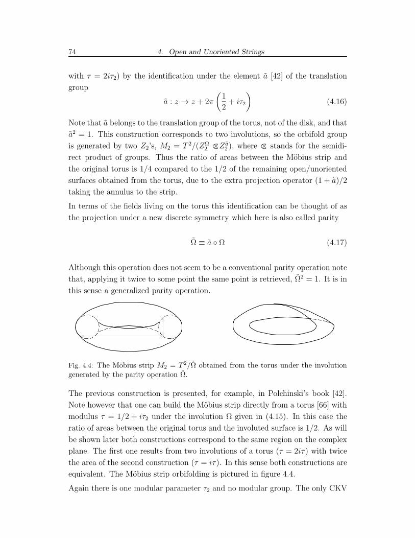
74 4. Open and Unoriented Strings
with τ = 2iτ2) by the identification under the element a [42] of the translation
group
a : z → z + 2π
(
1
2+ iτ2
)
(4.16)
Note that a belongs to the translation group of the torus, not of the disk, and that
a2 = 1. This construction corresponds to two involutions, so the orbifold group
is generated by two Z2’s, M2 = T 2/(ZΩ2 ⊂×Z a
2 ), where ⊂× stands for the semidi-
rect product of groups. Thus the ratio of areas between the Mobius strip and
the original torus is 1/4 compared to the 1/2 of the remaining open/unoriented
surfaces obtained from the torus, due to the extra projection operator (1 + a)/2
taking the annulus to the strip.
In terms of the fields living on the torus this identification can be thought of as
the projection under a new discrete symmetry which here is also called parity
Ω ≡ a Ω (4.17)
Although this operation does not seem to be a conventional parity operation note
that, applying it twice to some point the same point is retrieved, Ω2 = 1. It is in
this sense a generalized parity operation.
Fig. 4.4: The Mobius strip M2 = T 2/Ω obtained from the torus under the involutiongenerated by the parity operation Ω.
The previous construction is presented, for example, in Polchinski’s book [42].
Note however that one can build the Mobius strip directly from a torus [66] with
modulus τ = 1/2 + iτ2 under the involution Ω given in (4.15). In this case the
ratio of areas between the original torus and the involuted surface is 1/2. As will
be shown later both constructions correspond to the same region on the complex
plane. The first one results from two involutions of a torus (τ = 2iτ) with twice
the area of the second construction (τ = iτ). In this sense both constructions are
equivalent. The Mobius strip orbifolding is pictured in figure 4.4.
Again there is one modular parameter τ2 and no modular group. The only CKV

4.1. Riemann Surfaces:from Closed Oriented to Open and Unoriented 75
is again the translation in the imaginary direction.
The Klein bottle K2 is obtained from the torus with τ = 2iτ2 under the iden-
tification
z ∼= −z + 2πiτ2 (4.18)
This result is pictured in figure 4.5. The bottle is the involution of the torus
Fig. 4.5: The Klein bottle K2 = T 2/Ω′ obtained from the torus under the involutiongenerated by the parity operation Ω′.
K2 = T 2/ZΩ′
2 , which has a one parameter CKG with one CKV, translations in
the imaginary direction. There is one modulus τ2 and no modular group. The
resulting manifold has no boundary and no singular points but is unoriented.
Again a new parity transformation Ω′ can be defined
Ω′ : z → −z + 2πiτ2
z → −z + 2πiτ2
(4.19)
S2 P1 P2 T2 Ω Ω Ω′
z ↔ z z ↔ −1/z z ↔ −z a Ω z → −z + 2πiτ2z → −z + 2πiτ2
S2/P = D2 RP2 T 2/P = C2 M2 K2
C/O O/O C/U C/O O/O O/U C/U
Tab. 4.1: Parity operations for the topology T 2× [0, 1]. The torus geometry consideredis τ = iτ2 for Ω and τ = 2iτ2 for Ω and Ω′. Note that M2 can also be obtained fromthe torus with τ = 1/2 + iτ2 by considering the parity Ω. In the labels of the last linethe first letter stands for Open or Closed surface while the second letter stands forOriented or Unoriented.
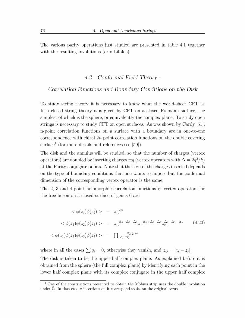
76 4. Open and Unoriented Strings
The various parity operations just studied are presented in table 4.1 together
with the resulting involutions (or orbifolds).
4.2 Conformal Field Theory -
Correlation Functions and Boundary Conditions on the Disk
To study string theory it is necessary to know what the world-sheet CFT is.
In a closed string theory it is given by CFT on a closed Riemann surface, the
simplest of which is the sphere, or equivalently the complex plane. To study open
strings is necessary to study CFT on open surfaces. As was shown by Cardy [51],
n-point correlation functions on a surface with a boundary are in one-to-one
correspondence with chiral 2n point correlation functions on the double covering
surface1 (for more details and references see [59]).
The disk and the annulus will be studied, so that the number of charges (vertex
operators) are doubled by inserting charges ±q (vertex operators with ∆ = 2q2/k)
at the Parity conjugate points. Note that the sign of the charges inserted depends
on the type of boundary conditions that one wants to impose but the conformal
dimension of the corresponding vertex operator is the same.
The 2, 3 and 4-point holomorphic correlation functions of vertex operators for
the free boson on a closed surface of genus 0 are
< φ(z1)φ(z2) > = z−2∆12
< φ(z1)φ(z2)φ(z3) > = z−∆1−∆2+∆3
12 z−∆1+∆2−∆3
13 z∆1−∆2−∆3
23
< φ(z1)φ(z2)φ(z3)φ(z4) > =∏
i<j z2qiqj/kij
(4.20)
where in all the cases∑
qi = 0, otherwise they vanish, and zij = |zi − zj|.The disk is taken to be the upper half complex plane. As explained before it is
obtained from the sphere (the full complex plane) by identifying each point in the
lower half complex plane with its complex conjugate in the upper half complex
1 One of the constructions presented to obtain the Mobius strip uses the double involutionunder Ω. In that case n insertions on it correspond to 4n on the original torus.

4.2. Conformal Field Theory -Correlation Functions and Boundary Conditions on the Disk 77
plane. In terms of correlation functions
〈φq(x, y)〉D2= 〈φq(z)φ−q(z)〉S2 (4.21)
where z = x+ iy was used in the the first equation of (4.20), y is the distance to
the real axis while x is taken to be the horizontal distance (parallel to the real
axis) between vertex insertions.
4.2.1 Dirichlet Boundary Conditions
As is going to be shown, when the mirror charges have opposite sign the boundary
conditions are Dirichlet.
The 2-point correlation function restricted to the upper half plane is simply the
expectation value
〈φq(x, y)〉 =1
(2y)2∆(4.22)
Insertion of vertex operators (except for the identity) on the boundary is not
compatible with the boundary conditions since the only charge that can exist
there is q = 0 (since q = −q = 0 on the boundary). Taking the limit y → 0
the expectation value (4.22) blows up but this should not worry us, since near
the boundary the two charges annihilate each other. This phenomena is nothing
else than the physical counterpart of the operator fusion rules φq(y)φ−q(−y) →(2y)−2∆φ0(y). That is, 〈φ0〉∂D2
= 〈1〉∂D2on the boundary of the disk.
3-point correlation functions cannot be used for the same reason, as one of the
insertions would need to lie on the boundary, but that would mean q3 = 0. The
other two charges would have to be inserted symmetrically with respect to the
real axis and this would imply q1 = −q2. This reduces the 3-point correlator to
a 2-point one in the full plane.
For 4-point vertex insertions consider q1 and q3 in the upper half plane, q2 (in-
serted symmetrically with respect to q1) and q4 (inserted symmetrically with
respect to q3) in the lower half plane. As pictured in figure 4.6, the most generic
configuration is q1 = −q2 = q and q3 = −q4 = q′. Taking z2 = z1 = −iy and
z4 = z3 = x − iy′ the corresponding 2-point correlators in the upper half plane

78 4. Open and Unoriented Strings
are obtained
〈φq(0, y)φq′(x′, y′)〉 = 1
(2y)2∆(2y′)2∆′
(
1− 4yy′
x2 + (y + y′)2
)2qq′
k
(4.23)
Again note that boundary operators cannot be inserted without changing the
boundary conditions. In the limit x → ∞ both correlators behave like
limx→∞
〈φ(y1)φ(y2)〉 =1
(4y1y2)2∆(4.24)
When the insertions approach the boundary the correlators go to infinity inde-
pendently of the value of x. This fact can be explained by the kind of boundary
conditions considered, since they are such that when the fields approach the
boundary they become infinitely correlated independently of how far they are
from each other. Therefore these must correspond to Dirichlet boundary con-
ditions, as the fields are fixed along the boundary, furthermore as stated before
their expectation value is 〈1〉. It doesn’t matter how far apart they are, they are
always correlated on the boundary. The tangential derivative to the boundary of
the expectation value ∂x 〈φ〉|∂D2= 0 also implies Dirichlet boundary conditions.
4.2.2 Neumann Boundary Conditions
For the case when the mirror charge has the same sign as the original one, the
boundary conditions will be Neumann. The expectation value for the fields in
the bulk vanishes since the 2-point function 〈φq(z1)φq(z2)〉 = 0 in the full plane.
Nevertheless, the non-zero 2-point correlation function on the boundary can be
directly evaluated
〈φq(0)φ−q(x)〉 =1
x2∆(4.25)
Note that contrary to the previous discussion, concerning Dirichlet boundary
conditions, in this case q 6= 0 on the boundary since the mirror charges have the
same sign and the correlation function vanishes in the limit x → ∞ indicating
that the boundary fields become uncorrelated.
The 3-point correlation function in the full plane must be considered with one
charge −2q on the boundary and two other charges q inserted symmetrically with
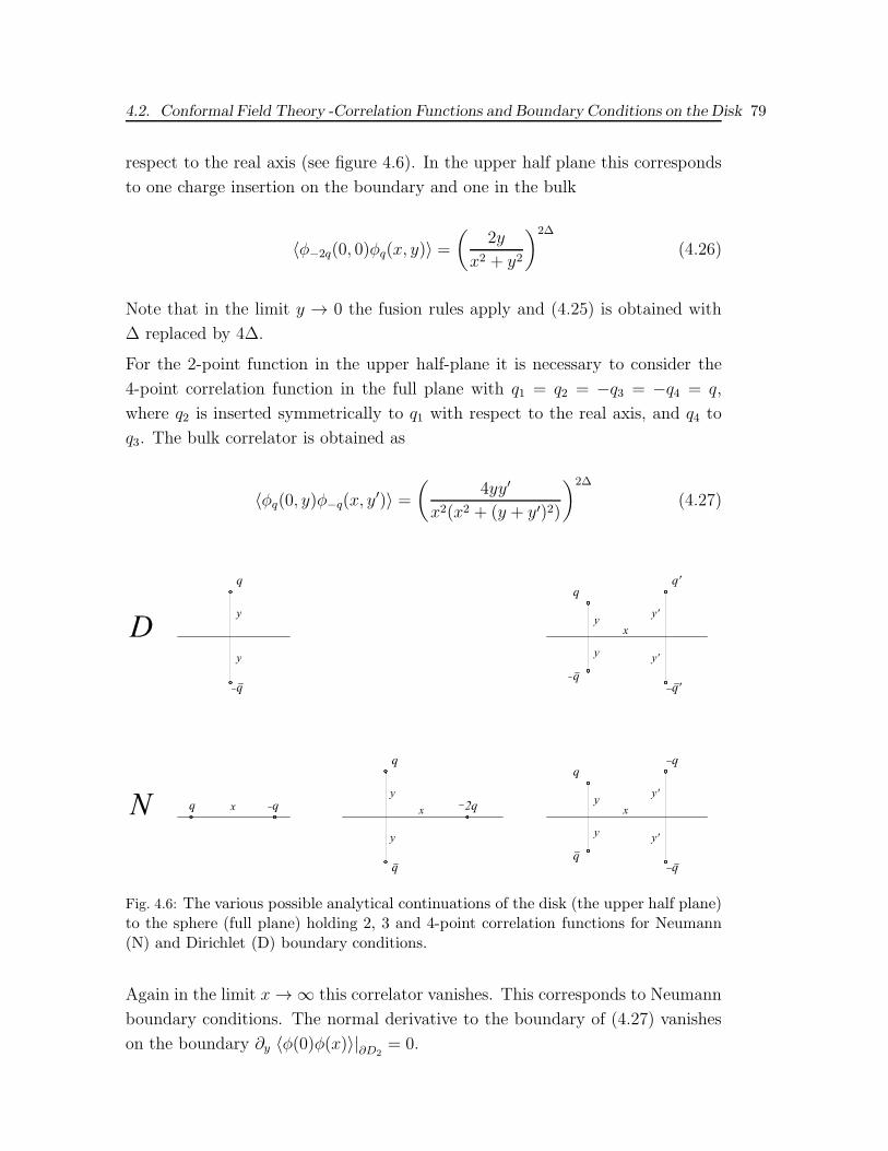
4.2. Conformal Field Theory -Correlation Functions and Boundary Conditions on the Disk 79
respect to the real axis (see figure 4.6). In the upper half plane this corresponds
to one charge insertion on the boundary and one in the bulk
〈φ−2q(0, 0)φq(x, y)〉 =(
2y
x2 + y2
)2∆
(4.26)
Note that in the limit y → 0 the fusion rules apply and (4.25) is obtained with
∆ replaced by 4∆.
For the 2-point function in the upper half-plane it is necessary to consider the
4-point correlation function in the full plane with q1 = q2 = −q3 = −q4 = q,
where q2 is inserted symmetrically to q1 with respect to the real axis, and q4 to
q3. The bulk correlator is obtained as
〈φq(0, y)φ−q(x, y′)〉 =
(
4yy′
x2(x2 + (y + y′)2)
)2∆
(4.27)
Fig. 4.6: The various possible analytical continuations of the disk (the upper half plane)to the sphere (full plane) holding 2, 3 and 4-point correlation functions for Neumann(N) and Dirichlet (D) boundary conditions.
Again in the limit x→ ∞ this correlator vanishes. This corresponds to Neumann
boundary conditions. The normal derivative to the boundary of (4.27) vanishes
on the boundary ∂y 〈φ(0)φ(x)〉|∂D2= 0.

80 4. Open and Unoriented Strings
For the case of one compactified free boson the process follows in quite a similar
way. The main difference resides in the fact that the right and left spectrum
charges are different. Taking a charge q = m+ kn/4 its image charge is now ±q,where q = m−kn/4. In this way it is necessary to truncate the spectrum holding
q = −q = kn/4 for Dirichlet boundary conditions, and q = q = m for Neumann
boundary conditions, in a pretty much similar way as happens in the Topological
Membrane. The results derived in this section are summarized in figure 4.6.
4.3 TM(GT)
Is now time to turn to the 3D TM(GT). In this section the results are derived
directly from the bulk theory and its properties. The derivations of the results
presented here are in agreement with the CFT arguments of the last section.
Initially only a single U(1) of type B TMGT corresponding to c = 1 CFT with
action given by (2.2) will be considered
S =
∫
M
dtd2z
[
−√−gγ
FµνFµν +
k
8πǫµνλAµFνλ
]
(4.28)
where, again, M = Σ × [0, 1] has two boundaries Σ0 and Σ1. Σ is taken to
be a compact manifold, t is in the interval [0, 1] and (z, z) stand for complex
coordinates on Σ.
As derived before upon quantization the charge spectrum is
Q = m+k
4n (4.29)
for some integers m and n as given by (2.40). Furthermore it has already been
proved [26,34] (see the previous chapter) that, for type B gauge groups and under
the correct relative boundary conditions, one insertion of Q on one boundary (cor-
responding to a vertex operator insertion on the boundary CFT) will, necessarily,
demand an insertion of the charge (2.41)
Q = m− k
4n (4.30)

4.3. TM(GT) 81
on the other boundary. This fact will be assumed through out the rest of this
chapter.
Our aim is to orbifold TM theory in a similar way to Horava [89], who obtained
open boundary world-sheets through this construction. A path integral approach
will be taken and the orbifold reinterpreted in terms of discrete PT and PCT
symmetries of the bulk 3D TM(GT).
4.3.1 Horava Approach to Open World-Sheets
Obtaining open string theories out of 3D (topological) gauge theories means
building a theory in a manifold which has boundaries (the 2D open string world-
sheet) that is already a boundary (of the 3D manifold). This construction raises
a problem since the boundary of a boundary is necessarily a null space. One
interesting way out of this dilemma is to orbifold the 3D theory, such that its
singular points work as the boundary of the 2D boundary. Horava [89] introduced
an orbifold group G that combines the world-sheet parity symmetry group ZWS2
(2D) with two elements 1,Ω, together with a target symmetry G of the 3D
theory fields
G ⊂ G× ZWS2 (4.31)
With this setup one can get three different kinds of constructions. Elements of
the kind h = h×1ZWS2
induce twists on the target space (not acting in the world-
sheet at all), for elements ω = 1G × Ω the world-sheet manifold is orbifolded
(giving an open world-sheet) without affecting the target space and for elements
g1 = g1 × Ω an exotic world-sheet orbifold is obtained. In this last case it is
further necessary to have an element corresponding to the twist in the opposite
direction g2 = g2×Ω. To specify these twists on some world-sheet it is necessary
to define the monodromies of fields on it. Taking the open string Co = C/Z2 as
the orbifold of the closed string C = S1
π1(Co) = D ≡ Z2 ∗ Z2 ≡ Z2 ⊂×Z (4.32)
with ∗ being the free product and ⊂× the semidirect product of groups. D is the in-
finite dihedral group, the open string first homotopy group. So the monodromies
of fields in Co correspond to a representation of this group in the orbifold group,

82 4. Open and Unoriented Strings
Z2 ∗ Z2 → G, such that the following triangle is commutative
Z2 ∗ Z2 −→ G
ց ւ
ZWS2
(4.33)
The partition function contains the sum over all possible monodromies
ZC(τ) =1
|G|∑
g1,g2,h
ZC(g1, g2, h; τ) (4.34)
where τ is the modulus of the manifold. The monodromies g1, g2 and h are
elements of G as previously defined satisfying g2i = 1 and [gi, h] = 1.
It will be shown that PCT plays the role of one of such symmetry with g1 = g2.
It is in this sense one of the most simple cases of exotic world-sheet orbifolds.
The string amplitudes can be computed in two different pictures. The loop-
channel corresponds to loops of length τ of closed and open strings and the
amplitudes are computed as traces over the Hilbert space. The tree-channel
corresponds to a cylinder of length τ created from and annihilated to the vacua
through boundary (|B〉) and/or crosscaps (|C〉) states. Comparing both ways for
the same amplitudes the following relations are obtained
Annulus (C2) : Tr open
(
e−Hoτ)
= 〈B| e−Hcτ |B〉
Mobius Strip (M2) : Tr open
(
Ωe−Hoτ)
= 12〈B| e−Hcτ |C〉+ 1
2〈C| e−Hcτ |B〉
Klein Bottle (K2) : Tr open
(
Ωe−Hoτ)
= 〈C| e−Hcτ |C〉(4.35)
These equations constitute constraints similar to the modular invariance con-
straints of closed string theories. The relation between the moduli are, for K2
and M2, τ = 1/(2τ), and for C2, τ = 2/(τ).
In terms of manifolds it is intended to obtain some open boundary Σo = Σ/I
(where boundary refers to M = Σ × [0, 1]) which is the involution under the

4.3. TM(GT) 83
symmetry I of its double cover, Σ. The resulting orbifolded manifold is
Mo = (Σ× [0, 1])/I (4.36)
where I acts in t as Time Inversion t → 1 − t. This construction is pictured in
figure 4.7.
Fig. 4.7: The thickened open string Co as an orbifold of the thickened closed string Cunder an I = Z2 symmetry. The boundaries of Co = C/ZWS
2 are the singular points ofthe orbifold.
In terms of the action and fields in the theory Horava used the same approach of
extending them to the doubled cover manifold
2So(Ao) = S(A) (4.37)
In simple terms, A stands for the extension of Ao fromMo to its double cover M .
Since there is a one-to-one correspondence between the quantum states of the
gauge theory on M and the conformal blocks of the WZWN model, the partition
function may be written as
ZΣ =∑
hijΨi ⊗ Ψj ∈ HΣ ⊗ HΣ (4.38)
where Ψi stands for a basis of the Hilbert space HΣ. The open string counterpart

84 4. Open and Unoriented Strings
in the orbifolded theory is
ZΣo=∑
aiΨi ∈ HΣ (4.39)
which also agrees with the fact that in open CFT’s the partition function is
the sum of characters (instead of the sum of squares) due to the fact that the
holomorphic and antiholomorphic sectors are not independent.
4.3.2 Discrete Symmetries and Orbifolds of TM(GT)
Following the discussion of section 4.1 and subsection 4.3.1, it becomes obvious
that the parity operation plays a fundamental role in obtaining open and/or non
orientable manifolds out of closed orientable ones, and hence open/unorientable
theories out of closed orientable theories.
Generally there are several ways of defining parity. The ones of interest have
already been presented here. For the usual ones, P1 and Ω defined in (4.4)
and (4.15), the fields of our 3D theory transform as
P1 : z ↔ z
Λ → Λ
A0 → A0
Az ↔ Az
Ez ↔ E z
B → −B
Q → Q
Ω : z ↔ −z
Λ → Λ
A0 → A0
Az ↔ −Az
Ez ↔ −E z
B → −B
Q → Q
(4.40)
where Λ is the gauge parameter entering into U(1) gauge transformations. Under
these two transformations the action transforms as
∫
(F 2 + kA ∧ F ) →∫
(F 2 − kA ∧ F ) (4.41)

4.3. TM(GT) 85
The theory is clearly not parity invariant. Let us then look for further discrete
symmetries which may be combined with parity in order to make the action
(theory) invariant. Introduce time-inversion, T : t → 1 − t, implemented in this
non standard way due to the compactness of time. Note that t = 1/2 is a fixed
point of this operation. Upon identification of the boundaries as described in [34]
the boundary becomes a fixed point as well.
It remains to define how the fields of the theory change under these symmetries.
There are two possible transformations compatible with gauge transformations,
AΛ(t, z, z) = A(t, z, z) + ∂Λ(t, z, z). They are:
CT : t → 1− t
Λ → Λ
A0 → −A0
A → A
E → −E
B → B
Q → Q
(4.42)
and
T : t → 1− t
Λ → −Λ
A0 → A0
A → −A
E → E
B → −B
Q → −Q
(4.43)
where C, charge conjugation, is defined as Aµ → −Aµ. This symmetry inverts
the sign of the charge, Q → −Q, as usual. These discrete symmetries together

86 4. Open and Unoriented Strings
with parity P or Ω are the common ones used in 3D Quantum Field Theory.
When referring to parity in generic terms the letter P will be used.
Under any of the T and CT symmetries the action changes in the same fashion
as it does for parity P given by (4.41). In this way any of the combinations PT
and PCT are symmetries of the action, S → S. Gauging them is a promising
approach to define the TM(GT) orbifolding. It is now clear why extra symmetries,
besides parity, are necessary in order to have combinations of them under which
the theory (action) is invariant. In general, whatever parity definition is used,
these results imply that PT and PCT are indeed symmetries of the theory.
It can be concluded straight away that any of the two previous symmetries ex-
change physically two boundaries working as a mirror transformation with fixed
point (t = 1/2, z = z = x) (corresponding actually to a line) as pictured in fig-
ure 4.8. It is considered that, whenever there is a charge insertion on one bound-
ary of q=m+kn/4, there exists an insertion of q = m−kn/4 on the other bound-
ary [24, 34].
Under the symmetries PT and PCT as given by (4.40), (4.42) and (4.43) the
boundaries will be exchanged as shown in figure 4.8. In the case of PCT the
charges will simply be swapped but in the case of PT their sign will change
q → −q. Note that Σ 1
2
= Σ(t = 1/2) only feels P or CP .
Fig. 4.8: Exchange of boundaries due to PT/PCT transformation.
As will be shown in detail there are important differences between the two sym-
metries CT and T , they will effectively gauge field configurations corresponding
to untwisted/twisted sectors of closed strings and Neumann/Dirichlet boundary
conditions of open strings.
Remembering that the final aim is to orbifold/quotient the theory by gauging

4.3. TM(GT) 87
the discrete symmetries, let us proceed to check compatibility with the desired
symmetries in detail. It is important to stress that field configurations satisfying
any PT/PCT combinations of the previous symmetries exist, in principle, from
the start in the theory. One can either impose by hand that the physical fields
obey one of them (as is usual in QFT) or it can be assumed that there is a wide
theory with all of these field configurations and obtain (self consistent) subtheories
by building suitable projection operators that select some types of configurations.
It is precisely this last construction that one must have in mind when building
several different theories out of one. In other words, several different new theories
are going to be built by gauging discrete symmetries of the type PCT and PT .
It is important to stress what the orbifold means in terms of the boundaries and
bulk from the point of view of TM(GT). It is splitting the manifold M into two
pieces creating one new boundary at t = 1/2. This boundary is going to feel
only CP or P symmetries since it is located at the temporal fixed point of the
orbifold. Figure 4.9 shows this procedure. In this way this new boundary is
Fig. 4.9: Orbifolding of TM(GT). Σ 1
2
only feels PT or P which are isomorphic to Z2
going to constrain the new theory in such a way that the boundary theories will
correspond to open and unoriented versions of the original full theory.
4.3.3 Tree Level Amplitudes for
Open and Closed Unoriented Strings
Let us start by considering tree level approximations to string amplitudes, i.e. the
Riemann surfaces are of genus 0. These surfaces are the sphere (closed oriented
strings) and its orbifolds: the disk (open oriented) and the projective plane (closed

88 4. Open and Unoriented Strings
unoriented) as was discussed in section 4.1. From the point of view of TM(GT),
orbifolding means that the manifoldM is split into two pieces that are identified.
As a result at t = 1/2, the fixed point of the orbifold, a new boundary is created.
For different orbifolds one will have different admissible field configurations. In
the following discussion we study those field configurations which are compati-
ble with PT and PCT type orbifolds for the various parity operations already
introduced.
Disk
Start from the simplest case - the disk. It is obtained by the involution of the
sphere under P1 as given by (4.4). So consider the identifications under P1CT
and P1T . For the first one the fields are transform as
P1CT : Λ(t, z, z) = Λ(1− t, z, z)
∂iEi(t, z, z) = −∂iEi(1− t, z, z)
B(t, z, z) = −B(1 − t, z, z)
Q(t) =
∫
Σ(t)
ρ0 = Q(1 − t) = −∫
Σ(1−t)
(−ρ0)
(4.44)
The orientations of Σ and Σ are opposite. Under these relations the Wilson lines
have the property
exp
iQ
∫
C
dxµAµ
= exp
iQ
∫
−C
dxµAµ
(4.45)
This means that for the configurations obeying the relations (4.44) the notion of
time direction is completely lost!
Under the involution of our 3D manifold, using the above relations as geometrical
identifications, the boundary is located at t = 0 and t = 1/2. For the moment
let us check the compatibility of the observables with the proposed orbifold con-
structions given by the previous relations. In a very naive and straightforward
way, when P1CT is used as given by (4.44) the charges should maintain their sign
(q(t) ∼= q(1− t)).

4.3. TM(GT) 89
Fig. 4.10: Orbifold under P1CT in the presence of 2 Wilson lines, Wq and W−q. Theyneed to pierce Σo 1
2
= S2/P1 = D2 on the real axis and the allowed charges are q = m.
Fig. 4.11: Orbifold under P1CT in the presence of 3 Wilson lines, W2q and two W−q.W2q must pierce Σo 1
2
= S2/P1 = D2 on the real axis and the allowed charges are q = m.

90 4. Open and Unoriented Strings
Then, in order for the exchange of boundaries to be possible, it is necessary
to truncate the spectrum and set q ∼= q = m for the identification to make
sense. Let us check what happens at the singular point of our orbifolded theory,
t = 1/2. The fields are identified according to the previous rules but the manifold
Σ(t = 1/2) = S2 is only affected by P1.
Take two Wilson lines that pierce the manifold in two distinct points, z and z′.
Under the previous involution P1CT , z is identified with z for t = 1/2. Then,
geometrically, the relation z′ = z must hold in order to have spatial identification
of the piercings. The problem is that when there are only two Wilson lines,
TM(GT) demands that they carry opposite charges. In order to implement the
desired identification q = 0 is the only possibility. For the case where the Wilson
lines pierce the manifold in the real axis, z = x and z′ = x′, the involution is
possible as pictured in figure 4.10 since the identification x ∼= x and x′ ∼= x′ is
considered.
In the presence of three Wilson lines, following the same line of argument, there
will necessarily exist one insertion on the boundary and two in the bulk as pictured
in figure 4.11. Only in the presence of four Wilson lines, as pictured in figure 4.12
can any insertion on the boundary be avoided.
Fig. 4.12: Orbifold under P1CT in the presence of 4 Wilson lines, two Wq and two W−q.The allowed charges are q = m.

4.3. TM(GT) 91
Note that the identification B(z, z) ∼= −B(z, z) on the real axis implies necessarily
B(x, x) = 0. Remember that 2πn =∫
B (see [26, 34] for details). It is possible
as well to have an insertion on the boundary and one in the bulk.
This fact is simply the statement that by imposing P1CT symmetry on the bulk
fields one is actually imposing Neumann boundary conditions in the CFT. The
charges of the theory become q = m, which means that the string spectrum has
only Kaluza-Klein momenta. Furthermore, the monopole induced processes are
suppressed. Recall that they change the charge by an amount kn/2 which would
take the charges out of the spectrum allowed in these configurations.
Following our journey consider next P1T . The fields now are related in the
following way
P1T : Λ(t, z, z) = −Λ(1− t, z, z)
∂iEi(t, z, z) = ∂iE
i(1− t, z, z)
B(t, z, z) = B(1− t, z, z)
Q =
∫
Σ(t)
ρ0 = −Q = −∫
Σ(1−t)(ρ0)
(4.46)
The Wilson line has the same property (4.45) as in the previous case.
Now the charges change sign under a P1T symmetry. As before identifying the
charges on opposite boundaries truncates the spectrum, q(t) ∼= −q(1− t). So, in
order to have compatibility with the orbifold, q ∼= −q = nk/4.
In this case two piercings in the 2D bulk can be identified since the charge
identification q ∼= −q is now compatible with the TM(GT) field configurations.
But no other operator than the identity φ0 can be inserted on the real axis
since the corresponding charge must be zero q(x) = −q(x) = 0. Therefore this
kind of orbifolding is only possible when there is an even number of Wilson
lines propagating in the 3D bulk. The result for two Wilson lines is pictured in
figure 4.13 and for four in figure 4.14.
In terms of the full theory, a new 2D boundary has been defined. It is a disk.
The piercings of Wilson lines are none other than the vertex operators (or fields)
of a Conformal Field Theory defined on that Disk. In this case B(z, z) = B(z, z),
so that B 6= 0 on the boundary.

92 4. Open and Unoriented Strings
Fig. 4.13: Orbifold under P1T in the presence of 2 Wilson lines, Wq and W−q. The newboundary is Σo 1
2
= S2/P1 = D2. The allowed charges are q = kn/4.
Fig. 4.14: Orbifold under P1T in the presence of 4 Wilson lines, Wq, W′q, W−q and W−q′ .
The new boundary is Σo 1
2
= S2/P1 = D2. The allowed charges are q = kn/4.

4.3. TM(GT) 93
So these facts translate into Dirichlet boundary conditions for P1T . The charges
allowed, are q = nk/4, the winding number of string theory. The monopole
induced processes are now allowed being crucial in this construction since they
allow the gluing on this new boundary of two Wilson lines carrying charges q =
nk/4 and q = −nk/4.
Projective Plane
Consider the parity operation as the antipodal identification given in (4.8). The
projective plane is obtained as the new 2D boundary of the orbifolded (under
this symmetry) membrane.
The transformation is given by
P2 : z → −1
z
z → −1
z
Λ(z, z) → Λ(−1
z,−1
z)
Az(z, z) → 1
z2Az(−
1
z,−1
z)
Az(z, z) → 1
z2Az(−
1
z,−1
z)
B(z, z) → 1
z2z2B(−1
z,−1
z)
Ez(z, z) → 1
z2Ez(−
1
z,−1
z)
Ez(z, z) → 1
z2Ez(−
1
z,−1
z)
(4.47)
Again the compatibility of the identifications under this new discrete symmetry
must be checked. Under t′ ∼= 1 − t, z′ ∼= −1/z and z′ ∼= −1/z we obtain, for

94 4. Open and Unoriented Strings
P2CT ,
P2CT : Λ(t, z, z) = Λ(1− t,−1z,−1
z)
∂iEi(t, z, z) = − 1
z2z2∂iE
i(1− t,−1z,−1
z)
B(t, z, z) = − 1z2z2
B(1− t,−1z,−1
z)
Q(t) =
∫
Σ(t)
ρ0 = Q(1 − t) = −∫
Σ(1−t)
(−ρ0)
(4.48)
Note that the relation between the integrals
∫
Σ(t′)
d2z′
z′2z′2z′2z′2
(
B(t′, z′, z′) + ∂iEi(t′, z′, z′)
)
=
∫
Σ(t)
d2z(
B(t, z, z) + ∂iEi(t, z, z)
)
(4.49)
follows from taking into account the second and third equalities of (4.48), and the
relations dz = dz′/z′2, dz = dz′/z′2, and consequently dz ∧ dz = −(1/z′2z′2)dz′ ∧dz′. Σ and Σ again have opposite orientations and are mapped into each other
by the given involution. Under these relations and in a similar way to (4.49) the
action transforms under P2 as given in (4.41) and any of the combinations P2CT
or P2T keep it invariant. Also the Wilson lines have the same property given
by (4.45).
In the derivation of the previous identifications (4.48) it was necessary to demand-
ing analyticity of the fields on the full sphere. This translates into demanding
that the transformation between the two charts covering the sphere be well de-
fined. Since ∂uΛ = −z2∂zΛ and ∂uΛ = −z2∂zΛ the fields must behave at infinity
and zero like
Λ∞→ z−1z−1 Λ
0→ z3z3
Az∞→ z−2z−1 Az
0→ z2z
Az∞→ z−1z−2 Az
0→ zz2
(4.50)
If naively one didn’t care about these last limits the relations would be plagued
with Dirac delta-functions coming from the identity 2πδ2(z, z) = ∂z(1/z) =
∂z(1/z). Once the previous behaviors are taken into account all these terms
will vanish upon integration. Another way to interpret these results is to note
that the points at infinity are not part of the chart (not physically meaningful).

4.3. TM(GT) 95
To check the physical behavior at those points it is necessary to compute it at
zero in the other chart.
This time the charges compatible with P2CT are q = m since q ∼= q. Once there
are no boundaries it is not possible to have configurations with two Wilson lines
which allow this kind of orbifold. In this way the smallest number of lines is four
as pictured in figure 4.15. Furthermore the total number of Wilson lines must be
even.
Fig. 4.15: Orbifold under PCT in the presence of 4 Wilson lines, two Wq and two W−q.The new 2D boundary is Σo 1
2
= S2/P = RP2. The allowed charges are q = m.
This configuration corresponds to untwisted closed unoriented string theories.
Note that Λ, which is identified with string theory target space, is not orbifolded
by P2CT . The charges allowed are q = m, the Kaluza-Klein momenta of string
theory. Once again the monopole processes are suppressed.
For P2T the fields transform as
P2T : Λ(t, z, z) = −Λ(1− t,−1z,−1
z)
∂iEi(t, z, z) = 1
z2z2∂iE
i(1− t,−1z,−1
z)
B(t, z, z) = 1z2z2
B(1− t,−1z,−1
z)
Q(t) =
∫
Σ(t)
ρ0 = −Q(1 − t) = −∫
Σ(1−t)
(−ρ0)
(4.51)
In this case q = kn/4 since q ∼= −q, and furthermore configurations with two
Wilson lines are compatible with the orbifold as pictured in figure 4.16.
In this case one obtains twisted unoriented closed strings. Note that the orbifold
identifies Λ ∼= −Λ such that the target space of string theory is orbifolded. The
full construction, including the world-sheet parity, from the point of view of string
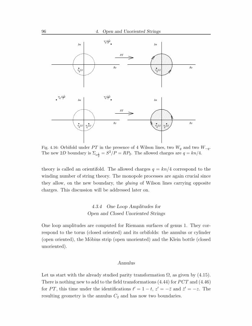
96 4. Open and Unoriented Strings
Fig. 4.16: Orbifold under PT in the presence of 4 Wilson lines, two Wq and two W−q.The new 2D boundary is Σo 1
2
= S2/P = RP2. The allowed charges are q = kn/4.
theory is called an orientifold. The allowed charges q = kn/4 correspond to the
winding number of string theory. The monopole processes are again crucial since
they allow, on the new boundary, the gluing of Wilson lines carrying opposite
charges. This discussion will be addressed later on.
4.3.4 One Loop Amplitudes for
Open and Closed Unoriented Strings
One loop amplitudes are computed for Riemann surfaces of genus 1. They cor-
respond to the torus (closed oriented) and its orbifolds: the annulus or cylinder
(open oriented), the Mobius strip (open unoriented) and the Klein bottle (closed
unoriented).
Annulus
Let us start with the already studied parity transformation Ω, as given by (4.15).
There is nothing new to add to the field transformations (4.44) for PCT and (4.46)
for PT , this time under the identifications t′ = 1− t, z′ = −z and z′ = −z. Theresulting geometry is the annulus C2 and has now two boundaries.

4.3. TM(GT) 97
Fig. 4.17: Orbifold under ΩCT in the presence of 2 and 4 Wilson lines. The new 2Dboundary is Σo 1
2
= S2/Ω = C2. The allowed charges are q = m.
For ΩCT the allowed charges are q = m due to the identification q ∼= q and
B(x) = 0 at the boundaries. There can exist two insertions on the boundaries of
the 2D CFT but not in its bulk due to the identifications of charges, basically
the argument is the same as that used for the disk. As on the disk there cannot
exist one single bulk insertion due to the total charge being necessarily zero in
the full plane. Up to configurations with four Wilson lines one can have: two
insertions on the boundary; one insertion in the bulk and one on the boundary
corresponding to three Wilson lines; three insertions on the boundaries (with∑
q = 0); one insertion in the bulk and two on the boundary corresponding to
four Wilson lines; and two insertions in the bulk corresponding to four Wilson
lines as pictured in figure 4.17.
This construction corresponds to open oriented strings with Neumann bound-
ary conditions. The charge spectrum is q = m, corresponding to Kaluza-Klein
momenta in string theory and the monopole induced processes are suppressed.
It is Neumann because the gauged symmetry is of PCT type. Note that the
definition of parity is not important, as even for genus 1 surfaces the results hold
similarly to the previous cases for P1 and P2 used in genus 0. What is important
is the inclusion of the discrete symmetry C!
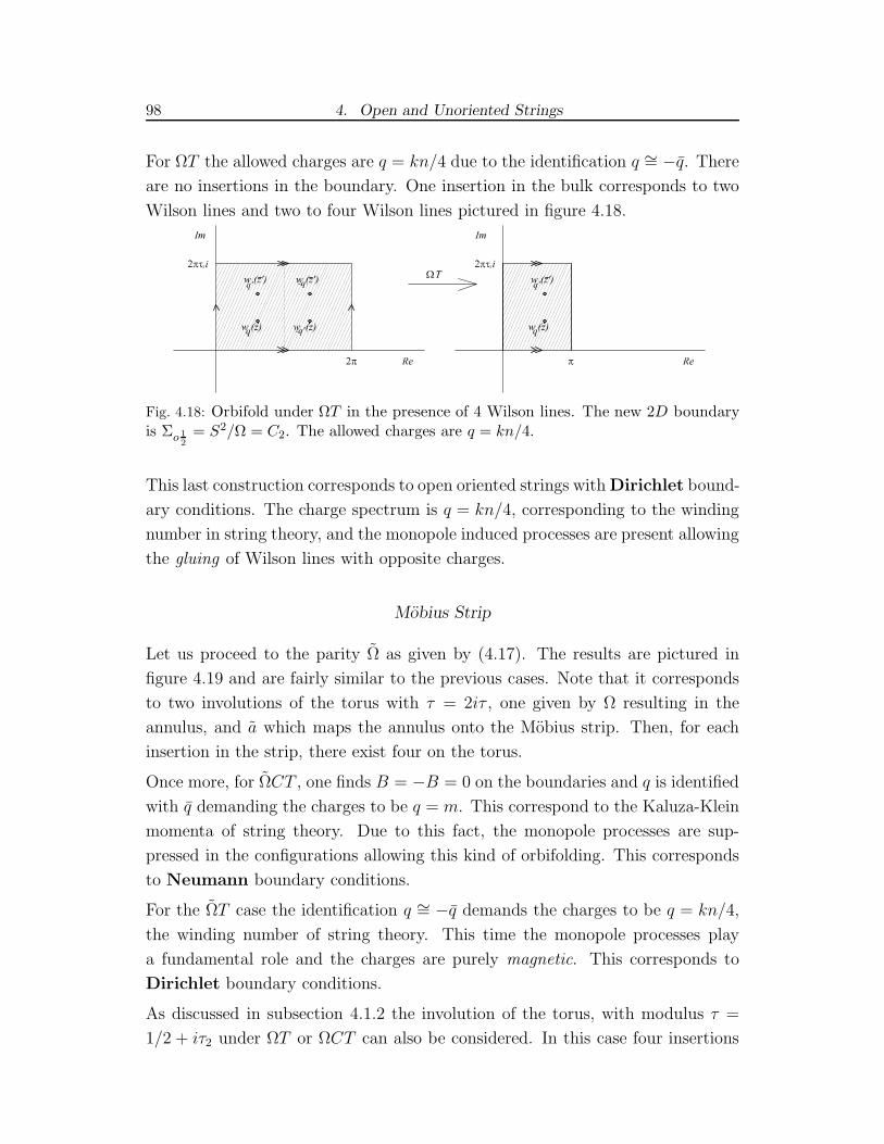
98 4. Open and Unoriented Strings
For ΩT the allowed charges are q = kn/4 due to the identification q ∼= −q. Thereare no insertions in the boundary. One insertion in the bulk corresponds to two
Wilson lines and two to four Wilson lines pictured in figure 4.18.
Fig. 4.18: Orbifold under ΩT in the presence of 4 Wilson lines. The new 2D boundaryis Σo 1
2
= S2/Ω = C2. The allowed charges are q = kn/4.
This last construction corresponds to open oriented strings withDirichlet bound-
ary conditions. The charge spectrum is q = kn/4, corresponding to the winding
number in string theory, and the monopole induced processes are present allowing
the gluing of Wilson lines with opposite charges.
Mobius Strip
Let us proceed to the parity Ω as given by (4.17). The results are pictured in
figure 4.19 and are fairly similar to the previous cases. Note that it corresponds
to two involutions of the torus with τ = 2iτ , one given by Ω resulting in the
annulus, and a which maps the annulus onto the Mobius strip. Then, for each
insertion in the strip, there exist four on the torus.
Once more, for ΩCT , one finds B = −B = 0 on the boundaries and q is identified
with q demanding the charges to be q = m. This correspond to the Kaluza-Klein
momenta of string theory. Due to this fact, the monopole processes are sup-
pressed in the configurations allowing this kind of orbifolding. This corresponds
to Neumann boundary conditions.
For the ΩT case the identification q ∼= −q demands the charges to be q = kn/4,
the winding number of string theory. This time the monopole processes play
a fundamental role and the charges are purely magnetic. This corresponds to
Dirichlet boundary conditions.
As discussed in subsection 4.1.2 the involution of the torus, with modulus τ =
1/2 + iτ2 under ΩT or ΩCT can also be considered. In this case four insertions

4.3. TM(GT) 99
Fig. 4.19: Orbifold under ΩT and ΩCT of the torus with τ = 2iτ2 in the presence offour Wilson lines. For ΩCT the Wilson lines may pierce the manifold on the real axisand the allowed charge is q = m. For ΩT , boundary insertions are not allowed and theadmissible charges are q = kn/4. The relation z′ = z + 2π(1/2 + iτ2) must hold.
on the torus correspond to two insertions on the strip as presented in figure 4.20
for the ΩT case.
Fig. 4.20: Orbifold under ΩT of the torus with τ = 1/2 + iτ2 in the presence of fourWilson lines.
As previously explained both constructions result in the same region of the com-
plex plane. Note that the resulting area in both cases is 2π2τ2 and that in both
cases the region [0, π]× i[0, 2πτ2] is identified with the region [π, 2π]× i[0, 2πτ2].
Klein Bottle
Finally using the parity Ω′ as given by (4.19), the points are identified under
t′ = 1 − t, z′ = −z + 2πiτ2 and z′ = −z + 2πiτ2. Upon orbifolding the new
boundary of TM is a Klein bottle.
Again, for Ω′CT , q = m is obtained because q ∼= q. The minimum number of

100 4. Open and Unoriented Strings
insertions is two corresponding to four Wilson lines in the bulk. This construc-
tion corresponds to untwisted unoriented closed strings with only Kaluza-Klein
momenta in the spectrum. The monopole processes are suppressed.
For Ω′T case the charge spectrum is truncated to q = kn/4 due to the iden-
tification q ∼= −q. One single insertion in the 2D bulk can also be obtained
corresponding to two Wilson lines or two insertions corresponding to four Wilson
lines. This construction corresponds to twisted unoriented closed strings with
only winding number. The monopole processes are present and are crucial in the
construction.
Fig. 4.21: Orbifold of Σ 1
2
= T 2 under Ω′CT and Ω′T .
Two examples corresponding to four Wilson lines are pictured in figure 4.21.
4.3.5 Note on Modular Invariance and the Relative Modular Group
Modular invariance is a fundamental ingredient in string theory which makes
closed string theories UV finite. What about the orbifolded theories? It is much
more tricky. Each separated sector of open and unoriented theories is clearly not
invariant under a modular transformation. The transformation τ → −1/2τ can
be interpreted as the exchange of the homology cycles α and β of the torus as
represented in figure 4.22. Equivalently it swaps PT and PCT orbifold types.
But then, if the first orbifold corresponds to the twisted sector (closed unoriented

4.3. TM(GT) 101
strings) or to Dirichlet boundary conditions (open strings), the second orbifold
will correspond to the untwisted sector (closed unoriented strings) or to Dirichlet
boundary conditions (open strings). Note the sign of the charges in figure 4.22
representing the Klein bottle projection.
Fig. 4.22: A suitable modular transformation takes us from one projection PT (orbifold)to the other one PCT .
So if one actually wants to ensure modular invariance it is necessary to build a
projection operator which ensures it. A good choice would be
O =2 + PT + PCT
4(4.52)
such that the exchange of orbifolds doesn’t change it. This fact is well known in
string theory (see [42] for details).
In the case that the orbifolded manifolds result in open surfaces the modu-
lar transformation τ → −1/τ , according to the previous discussion, exchanges
the boundary conditions (Neumann/Dirichlet). Note that orbifolding the target
space in string theory (or equivalently the gauge group in TMGT) is effectively
creating an orientifold plane where the boundary conditions must be Dirichlet
(as for a D-brane). This is the equivalent of twisting for open strings. In terms of
the bulk the modular transformation is exchanging the projections PCT ↔ PT .
Putting it in more exact terms, consider some discrete group H of symmetries
of the target space (or equivalently the gauge group of TMGT). Consider now
the twist by the element h = (h1, h2) ∈ H , where h1 twists the states in the
x1 direction and h2 in the x2 direction. Then the modular transformation will

102 4. Open and Unoriented Strings
change the twist as
T : τ → τ + 1 (h1, h2) → (h1, h1h2)
S : τ → −1
τ(h1, h2) → (h2, h
−11 )
(4.53)
Returning to the Horava picture of describing an open string as a thickened surface
(or double cover), in the case of the orbifold resulting in a new open boundary
the picture is similar. In this case a modular transformation takes an open string
loop, with the ends attached to the boundaries (direct-channel picture) to a closed
string propagating from boundary to boundary (transverse-channel picture) as
pictured in figure 4.23 for the annulus.
Fig. 4.23: A suitable modular transformation takes us from the direct-channel pictureto the transverse-channel picture. Here this construction is pictured in terms of thethickened string.
The lower boundary of the membrane is a thickening of the string. In the case
of the open string loop one can imagine that the open string, while propagating,
splits into two parts. The left modes propagate in the top half of the torus while
the right modes propagate in the bottom half of the torus. In the case of the
closed string, there is again a splitting of the closed string exactly as before but
the propagation of the modes is transverse to the previous case as pictured in
figure 4.23.
Basically this discussion explains relations (4.35). The direct channel-picture on

4.3. TM(GT) 103
the disk correspond to Tr open
(
e−Hoτ)
where the trace is considered over the
possible Chan-Paton factors carried by the open string. The transverse-channel
picture corresponds to⟨
B∣
∣e−Hoτ∣
∣B⟩
where |B〉 stands for the states of the closedstring.
So far only one loop amplitudes were considered, i.e. genus 1 world-sheet surface
orbifolds. For the pure bosonic case this is sufficient, but once fermions and
supersymmetry are introduced new constraints emerge in two loop amplitudes.
Specifically the modular group of closed Riemann surfaces at genus g is SL(2g,Z),
upon orbifolding there is a residual conformal group, the so called Relative
Modular Group [83] (see also [84–86]). For genus 1 this group is trivial but for
higher genus it basically mixes neighboring tori. This means it mixes holes and
crosscaps (note that any surface of higher genus can be obtained from sewing
genus 1 surfaces). Furthermore, the string amplitudes defined on these genus 2
open/unoriented surfaces must factorize into products of genus 1 amplitudes. For
instance a 2 torus amplitude can be thought as two 1 torus amplitudes connected
through an open string. For a discussion of the same kind of constraints for closed
string amplitudes see [77–81].
The factorization and modular invariance of open/unoriented superstring theory
amplitudes will induce generalized GSO projections ensuring the consistency of
the resulting string theories.
The correct Neveu-Schwarz (NS - antiperiodic conditions, target spacetime fermions)
and Ramond (R - periodic conditions, target spacetime bosons) sectors were
built from TMGT in [30]. There the minimal model given by the coset Mk =
SU(2)k+2 × SO(2)2/U(1)k+2 with the CS action
SN=2[A,B,C] = kSCSSU(2)[A] + 2SCS
SO(2)[B]− (k + 2)SCSU(1)[C] (4.54)
was considered. It induces, on the boundary, an N = 2 Super Conformal Field
Theory (see also [27] for N = 1 SCFT). The boundary states of the 3D theory
corresponding to the NS and R sectors are obtained as quantum superpositions
of the 4 possible ground states (wave functions corresponding to the first Landau
level - the ground state is degenerate) of the gauge field B, that is to say it is
necessary to choose the correct basis of states. The GSO projections emerge in
this way as some particular superposition of those 4 states at each boundary (for
further details see [30]). It still remains to see how these constraints emerge from

104 4. Open and Unoriented Strings
genus 2 amplitudes from TM and its orbifolds but this issue is not going to be
addressed in this work.
4.3.6 Neumann and Dirichlet World-Sheet Boundary Conditions,
Monopole Processes and Charge Conjugation
It is clear by now that the operation of charge conjugation C is selecting im-
portant properties of the new gauged theory. This means the properties of the
2D boundary string theory. Gauging PCT results in having an open CFT with
Neumann boundary conditions, while gauging PT results in having Dirichlet
boundary conditions. So C effectively selects the kind of boundary conditions!
In the case that PCT gives a closed unoriented manifold, an untwisted theory
is obtained, while for PT a twisted theory is obtained (orientifold X ∼= −X).
Again C effectively selects the theory to be twisted or not. These results are
summarized in table 4.2.
P1 P2 Ω Ω Ω′
S2 → D2 RP2 T 2 → C2 M2 K2
O/O C/U O/O O/U C/U
CT N Untwisted N N Untwistedq=m q=m q = m q = m q=m
T D Twisted D D Twistedq = kn/4 q = kn/4 q = kn/4 q = kn/4 q = kn/4
Tab. 4.2: Boundary conditions and twisted sectors.
Although these facts are closely related with string T-duality, the C operation
does not give us the dual spectrum. Upon gauging the full theory it only selects
the Kaluza-Klein momenta or winding number as the spectrum of the configura-
tions being gauged.
From the point of view of the bulk theory the gauged configurations corresponding
to Neumann boundary conditions correspond to two Wilson lines with one end
attached to the 1D boundary of the new 2D boundary of the membrane at t = 1/2
and the other end attached to the 2D boundary at t = 0. For Dirichlet boundary
conditions there is one single Wilson line with both ends in the 2D membrane

4.3. TM(GT) 105
boundary at t = 0 and a monopole insertion in the bulk of the 2D boundary at
t = 1/2. Note that the Wilson lines no longer have a well defined direction in
time: time inversion has been gauged. These results are presented in figure 4.24.
Fig. 4.24: For Dirichlet boundary conditions two Wilson lines carrying charges q and−q meet in a monopole at the orbifold singular point t = 1/2. For Neumann boundaryconditions the two Wilson lines end on the boundary of Σ/Z2.
For the case where unoriented manifolds are obtained the picture is quite similar.
There are always an even number of bulk insertions. In the case of PCT the
Wilson lines which are identified have the same charge, therefore there are no
monopole processes involved. The two Wilson lines are glued at t = 1/2 becoming
in the orbifolded theory one single line which has both ends attached to Σ0 and
one point in the middle belonging to Σ1/2. In the boundary CFT it corresponds
to two vertex insertions with opposite momenta. This construction corresponds
to untwisted string theories since the target space coordinates (corresponding to
the gauge parameter Λ in TM(GT)) are not orbifolded.
In the case of PT the identification is done between charges of opposite signs.
Then two Wilson lines become one single line with its ends attached to Σ0,
but at one end they have a charge q and at the other end they have a charge
−q. In Σ1/2 there is a monopole insertion which changes the sign of the charge.
This construction corresponds to twisted string theories since the target space
coordinates are orbifolded (Λ ∼= −Λ).
As a final consistency check, in PCT type of orbifolds the charges are always
restricted to be q = m due to compatibility with the orbifold construction. By
restricting the spectrum to this form one is actually eliminating the monopole

106 4. Open and Unoriented Strings
processes for these particular configurations!
4.3.7 T-Duality and Several U(1)’s
The well know Target space or T-duality (for a review see [60]) of string theory
is a combined symmetry of the background and the spectrum of momenta and
winding modes. It interchanges winding modes with Kaluza-Klein modes. From
the point of view of the orbifolded TM(GT) corresponding to open and unoriented
string theories the projections PT truncate the charge spectrum to q = kn/4
(due to demanding q = −q) which in string theory is the winding number. The
projections PCT truncate the charge spectrum to q = m (due to demanding
q = q) which corresponds in string theory to the Kaluza-Klein momenta. Note
that PCT excludes all the monopole induced processes while PT singles out only
monopole induced processes [26, 31, 34].
T-duality is, from the point of view of the 3D theory, effectively exchanging the
two kinds of projections
T− duality : PT ↔ PCT
q = −q ↔ q = q(4.55)
This is precisely what it must do. The nature of duality in 3D terms was dis-
cussed in some detail in [29]. It was shown there that it exchanges topologically
non-trivial matter field configurations with topologically non trivial gauge field
configurations. Although charge conjugation was not discussed there (only parity
and time inversion), this mechanism can be thought of as a charge conjugation
operation. Note that C2 = 1.
It is also rather interesting that from the point of view of the membrane both
T-duality and modular transformations are playing the same role. In some sense
both phenomena are linked by the 3D bulk theory.
So far only a single U(1) theory with gauge fields obeying B boundary conditions
was considered. But new phenomena emerge in the more general case. The extra
B gauge sectors are necessary any how [34].
Take then the general action with gauge group U(1)d × U(1)D with d type B
4.3. TM(GT) 107
gauge fields and the remaining D gauge fields of type B,
Sd+D =
∫
M
dx3[
−√−gγ
(
FMµνF
µνM + F I
µνFµνI
)
+ǫµνλ
8π
(
KMNAMµ ∂νA
Nλ +KIJA
Iµ∂νA
Jλ
)
]
(4.56)
whereM,N = 1, . . . , d correspond to type B gauge fields and I, J = d+1, . . . , d+
D to type B fields.
For a given parity P , one can build an operator O that acts on every A field
through PT and only on some of them through C
O = PT
(
∑
I′
CδI′I +∑
I′′
δI′′I
)
(4.57)
Due to the charges not being quantized and the non-existence of monopole-
induced processes in the B gauge sector, the mechanism is slightly different (see
section 4.2). But this operator can act as well over the B sector.
For the case of open manifolds M/PT , I ′ runs over the indices for which one
wants to impose Neumann boundary conditions (on ΛI′) and I ′′ over the indices
corresponding to Dirichlet boundary conditions. For the case of closed manifolds
M/PT the picture is similar but I ′ runs over the indices for which one wants ΛI′
to be orbifolded (obtaining an orientifold or twisted sector).
In the case of several U(1)’s more general symmetries (and therefore orbifold
groups) can be considered (for instance ZN). Those symmetries are encoded in
the Chern-Simons coefficient KIJ .

108 4. Open and Unoriented Strings

5. FINAL REMARKS
The work presented here is one further step towards the description of string
theory from TM. Most of the constraints on string theories exist because of
their intimate relations to 2D geometry, 2D conformal field theories and their
symmetries. One of these constraints is modular invariance which puts severe
restrictions on the spectrum of the theories. Modular invariance, as employed by
Narain in the context of toroidal compactification, reduces the physical problem of
finding the allowed momenta and winding modes in string theory to the problem
of constructing lattices on a pseudo-Euclidean space RdR,dL on which physical
invariants are modular invariant functions. These lattices turn out to be self-
dual, integer and even lattices.
In Chapter 3 the results of Narain compactification were reproduced starting
from 3D gauge dynamics without referring to modular invariance at all. The
fact that 3D topologically massive gauge theory carries full information about
the lattices of string theory is quite fascinating. The approach presented here
and the modular invariance construction are compatible and moreover they are
logically connected. But there is still an element of surprise here because of the
crucial difference between the ideology of these two approaches. To see this let
us summarize what has been obtained so far. The starting point is a TMGT
defined on a three manifold with two disconnected boundaries. Gauge degrees
of freedom became dynamical on the boundaries generating chiral CFT’s. Each
boundary of the three manifold is interpreted as a “chiral worldsheet” of string
theory, meaning that the left and right modes are physically separated. This is
the framework of Topological Membrane theory. The Abelian theory with fields
of type B which has a discrete charge spectrum of the form Q = m+ kn/4 was
considered. A particle with charge Q is inserted at one boundary and it travels
through the bulk, interacts with all possible charge violating instantons on its
path and links with other charges and emerges as a new charge Q = m − kn/4
on the other boundary. The path of the charged particle is represented by a
110 5. Final Remarks
Wilson line in the bulk theory. After taking care of all the linkings and instanton
interactions it is quite an amusing result to obtain that the emerging charge in the
other boundary is of the Q form and nothing else. The Aharonov-Bohm phases
of the linkings interfere in such a way that for a particle which does not have the
charge ±Q there is zero probability to emerge at the other boundary. Moreover
a natural self-dual Lorentzian lattice structure emerges from the linkings of the
Wilson lines as was shown in Chapter 3. The connection between this approach
and the modular invariance arguments was not worked out here, but naively one
can see that modular transformations at the boundaries will yield linkings of the
Wilson lines in the bulk. This is why these results were obtained.
Chapter 4 has also shown how one can obtain open and closed unoriented string
theories from the Topological Membrane. There were two major ingredients: one
is the Horava idea about orbifolding, the second is that the orbifold symmetry
was a discrete symmetry of TMGT. The orbifold works from the point of view of
the membrane as a projection of field configurations obeying either PT or PCT
symmetries (the only two kinds of discrete symmetries compatible with TMGT).
For PCT type projections, Neumann boundary conditions were obtained for
open strings, and untwisted sectors for closed unoriented strings. For PT type
projections Dirichlet boundary conditions were obtained for open strings, and
twisted sectors for closed unoriented strings. For PCT , q = q = m, so only the
string Kaluza Klein modes survive. In this case the monopole induced processes
are completely suppressed. For PT , q = −q = kn/4, so only the string winding
modes survive. In this case only monopole induced processes are present, the
charges being purely magnetic. Charge conjugation C plays an important role in
all these processes, playing the role of a Z2 symmetry of the string theory target
space. These results can be generalized to symmetries of the target space encoded
in the tensor KIJ and are closely connected. Both to modular transformations
and T-duality which exchange PT ↔ PCT .
As a final remark note that the string photon Wilson line has been left out.
TM(GT) can take account of it as well: for any closed Σ there is a symmetry of
the gauge group coupling tensor KIJ → KIJ+δIχJ−δJχI where each χI = χI [A]
is taken to be some function of the AI ’s. This transformation affects only BIJ
and the induced terms vanish upon integration by parts. Once the orbifold of the
theory is considered, the new orbifolded Σo has a boundary and the induced terms
will no longer vanish. Instead they will induce a new action on the boundary ∂Σo.
This will be precisely the new gauge photon action of open string theories. As is
111
well known the choice of the gauge group of string theory, i.e. the Chan-Paton
factor structure carried by this photon Wilson line, will be determined by the
cancellation of the open string theory gauge anomalies (see [42] and references
therein).
There are a couple of important things which need to be addressed in the fu-
ture. The proper treatment of the string photon Wilson line [92] will allow the
introduction of D-branes in the context of TM constituting a promising field of
research connected with this last subject.
Another work would be the bulk interpretation of A-D-E classification [61] of
modular invariant partition functions on the boundary [11–13, 63, 64]. Also, re-
lated to these modular invariants, one would like to derive the orbifolded partition
functions of the boundary CFT from the bulk TMGT [92].
Although it was shown that the charge conjugation symmetry C plays an im-
portant role both in modular invariance and in T-duality, neither of them have
been properly studied. To properly describe modular invariance it is necessary
to take the gravitational diffeomorphisms due to the TMG sector into account.
Also, so far the full duality group [60] has not been properly described in terms
of symmetries of the 3D QFT, although a study has been done in [28, 29].
Concerning the generalized GSO projections of subsection 4.3.5 it still remains
to study how they emerge from genus 2 amplitudes from the point of view of TM
and its orbifolds.
Also an issue to address in future work will be to generalize the orbifold con-
structions presented here to non-trivial boundary CFT’s, for example WZWN
models and different coset models which can be obtained from the TM with a
non-Abelian TMGT.
Some further interesting directions of research are to obtain boundary CFT loga-
rithmic theory [93] and deriving the Sen mechanism [94] (tachyon condensation)
from the TM (see [32] for an initial study). These aspects are vital if one wants
to build consistent effective non supersymmetric string theories.
Finally the framework presented in this work can be applied to other quantum
theories which include the CS term such as the effective Quantum Hall Effect.
For example in [95] is studied the Jain hierarchy using such a theory.

112 5. Final Remarks

BIBLIOGRAPHY
[1] S.-S. Chern and J. Simons, Characteristic Forms and Geometric Invariants,
Ann. Math. 99 (1974) 48
[2] A. Schwarz, The Partition Function of Degenerate Quadratic Functional
and Ray-Singer Invariants, Lett. Math. Phys. 2 (1978) 247
[3] W. Siegel, Unextended Superfields in Extended SuperSymmetry, Nucl. Phys.
B156 (1979) 135
[4] R. Jackiw and S. Templeton, How Super-Renormalizable interactions Cure
Their Infrared Divergences, Phys. Rev. D23 (1981) 2291
[5] J. Schonfeld,A Mass Term for Three-dimensional Gauge Fields, Nucl. Phys.
B185 (1981) 157
[6] S. Deser, R. Jackiw and S. Templeton, Three-Dimensional Massive Gauge
Theories, Phys. Rev. Lett. 48 (1982) 975-978; Topologically Massive Gauge
Theories, Ann. Phys. NY 140 (1982) 372-411
[7] S. Deser, Physico-Mathematical Interactions: The Chern-Simons Story,
Contribution to proceedings to the 65th anniversary of L.D. Faddeev, math-
ph/9812005
[8] E. Witten, Quantum Field Theory and the Jones Polynomial, Commun.
Math. Phys. 121 (1989) 351-399
[9] G. Moore and N. Seiberg, Taming the Conformal Zoo, Phys. Lett. B220
(1989) 422
[10] S. Elitzur, G. Moore, A. Schwimmer and N. Seiberg, Remarks on the
Canonical Quantization of the Chern-Simons-Witten Theory, Nucl. Phys.
B326 (1989) 108
114 Bibliography
[11] M. Bos and V. P. Nair, U(1) Chern-Simons Theory and c = 1 Conformal
Blocks, Phys. Lett. B223 (1989) 61; Coherent State Quantization of Chern-
Simons Theory, Int. J. Mod. Phys. A5 (1990) 959
[12] J. M. F. Labastida and A. V. Ramallo, Operator Formalism for Chern-
Simons Theories, Phys. Lett. B227 (1989) 92; Chern-Simons Theory and
Conformal Blocks, Phys. Lett. B228 (1989) 214
[13] W. Ogura, Path Integral Quantization of Chern-Simons Gauge Theory,
Phys. Lett B229 (1989) 61
[14] G. Dunne, Aspects of Chern-Simons Theory, hep-th/9902115
[15] E. Witten, String Theory Dynamics in several Dimensions, Nucl. Phys.
B443 (1995) 85-126
[16] P.K. Townsend, The Eleventh-Dimension Membrane Revisited, Phys. Lett.
B350 (1995) 184-187
[17] E. Witten, Non-Commutative Geometry and String Field Theory, Nucl.
Phys. B268 (1986) 253-294
[18] I. I. Kogan, The Off-Shell Closed String as Topological Open Membranes.
Dynamical Transmutation of World Sheet Dimension, Phys. Lett. B231
(1989) 377
[19] S. Carlip and I. I. Kogan, Quantum Geometrodynamics of the Open Topo-
logical Membrane and String Moduli Space, Phys. Rev. Lett. 64 (1990) 1487;
Three-Dimensional Gravity and String Ghosts, Phys. Rev. Lett. 67 (1991)
3647-3649
[20] S. Carlip and I. I. Kogan, Three-Dimensional Topological Field Theories
and Strings, Mod Phys. Lett. A6, No 3 (1991) 171-181
[21] I. I. Kogan, Quantum Mechanics on the Moduli Space from the Quantum
Geometrodynamics of the Open Topological Membrane, Phys. Lett. B256
(1991) 369;Quantum Liouville Theory from Topological Massive Gravity:
1+1 Cosmological Constant as Square of 2+1 Graviton Mass, Nucl. Phys.
B375 (1992) 362
[22] S. Carlip, Inducing Liouville Theory from Topological Massive Gravity,
Nucl. Phys. B362, No 3 (1991) 111-124

Bibliography 115
[23] S. Carlip, (2 + 1)-Dimensional Chern-Simons Gravity as a Dirac Square
Root, Phys. Rev. D45 (1992) 3584-3590
[24] L. Cooper and I. I. Kogan, Boundary Conditions and Heterotic Construc-
tion in Topological Membrane Theory, Phys. Lett. B383 (1996) 271-280
[25] G. Amelino-Camelia, I. I. Kogan and R. J. Szabo, Conformal Dimen-
sions from Topologically Massive Quantum Field Theory, Nucl. Phys. B480
(1996) 413-456; Gravitational Dressing of Aharonov-Bohm Amplitudes,
Int.J.Mod.Phys. A12 (1997) 1043-1052
[26] L. Cooper, I. I. Kogan and K.M. Lee, String Winding Modes from Charge
Non-Conservation in Compact Chern-Simons theory, Phys.Lett. B394
(1997) 67-74
[27] I. Kogan, Three-Dimensional Description of the Phi(1,3) Deformation of
Minimal Models, Phys. Lett. B390 (1997) 189-196
[28] L. Cooper, The Topological Membrane Approach to String Theory, D.Phil
Thesis, 1997
[29] L. Cooper, I. I. Kogan and R. J. Szabo, Mirror Maps in Chern-Simons
Gauge Theory, Annals. Phys. 268 (1998) 61-104
[30] L. Cooper, I. I. Kogan and R. J. Szabo, Dynamical Description of Spectral
Flow in N = 2 Superconformal Field Theories, Nucl. Phys. B498 (1997)
492-510
[31] I. I. Kogan and R. J. Szabo, Liouville Dressed Weights and Renormalization
of Spin in Topologically Massive Gravity, Nucl.Phys. B502 (1997) 383-418
[32] I. I. Kogan and A. Lewis, Vacuum Instability in Chern-Simons Theory, Null
Vectors and Two-Dimensional Logarithmic Operators, Phys. Lett. B431
(1998) 77-84
[33] I. I. Kogan, A. Momen and R. J. Szabo, Induced Dilaton in Topologically
Massive Quantum Field Theory, JHEP 9812 (1998) 013
[34] P. Castelo Ferreira, I. I. Kogan and Bayram Tekin, Toroidal Compactifi-
cation in String Theory from Chern-Simons Theory, Nucl. Physics B589
(2000) 167-195

116 Bibliography
[35] P. Castelo Ferreira and I. I. Kogan, Open and Unoriented Strings from
Topological Membrane. I Prolegomena, JHEP 06 (2001) 056
[36] For a review see Lectures on Topological Membranes
in Campos do Jordao (1997) Particles and fields 223-290
http://www-thphys.physics.ox.ac.uk/users/IanKogan/membrane.ps
[37] M Crescimanno and S. A. Hotes, Monopoles, Modular Invariance and
Chern-Simons Field Theory, Nucl. Phys. B372 (1992) 683-700
[38] S. Deser and X. Xiang, Canonical Formulations of Full Nonlinear Topolog-
ical Massive Gravity, Phys. Lett. B263 (1991) 39-43
[39] E. Witten, 2 + 1 Dimensional Gravity as an exactly Soluble System, Nucl.
Phys. B311 (1988/89) 46-78
[40] H. Verlinde, Conformal Field Theory, 2-Dimensional Gravity and Quanti-
zation of Teichmuller Space, Nucl. Phys. B337 (1990) 652
[41] A. Alekseev and S. Shatashvili, Path Integral Quantization of the Coadjoint
orbits of the Virasoro Group and 2−D Gravity, Nucl. Phys. B323 (1989)
719
[42] J. Polchinski, String Theory, Cambridge University Press
[43] I. Kogan and D. Polyakov, World Sheet Logarithmic CFT in AdS Strings,
Ghost Matter Mixing and M-Theory, Int. J. Mod. Phys. A16 (2001) 2559-
2576
[44] K. Lee, Charge Violation by Instantons in Chern-Simons Theories, Nucl.
Phys. B373 (1992) 735-748
[45] P. Ning-Tan, B. Tekin and Y. Hosotani, Spontaneous Symmetry Breaking at
two loop in 3-D Massless Scalar Electrodynamics, Phys. Lett. B388 (1996)
611-620;Maxwell Chern-Simons Scalar Electrodynamics at Two Loop, Nucl.
Phys. B502 (1997) 483-515
[46] K. S. Narain, New Heterotic String Theories in Uncompactified Dimensions
< 10, Phys. Lett. B169 (1986) 41
[47] K. S. Narain, M. H. Samardi and E. Witten, A Note on Toroidal Compact-
ification of Heterotic String Theory, Nucl. Phys. B279 (1987) 369

Bibliography 117
[48] D. Gross, J. Harvey, E. Martinec and R. Rohm, Heterotic String. 1. The
Free Heterotic String, Nucl. Phys. B256 (1985) 253
[49] D. Gross, J. Harvey, E. Martinec and R. Rohm, Heterotic String. 2. The
Interacting Heterotic String, Nucl. Phys. B267 (1986) 75
[50] A. A. Belavin, A. M. Polyakov and A. B. Zamoldchikov, Infinite Conformal
Symmetry of Critical Fluctuations in Two-Dimensions , J. Stat. Phys. 34
(1984) 753; Infinite Conformal Symmetry in Two-Dimensional Quantum
Field Theory, Nucl. Phys. B241 (1984) 333-380
[51] J. L. Cardy, Conformal Invariance and Universality in Finite Size Scaling,
Nucl. Phys. B240[FS12] (1984) 514-532
[52] Vl. S. Dotsenko, Critical Behavior and Associated Conformal Algebra of
the Z(3) Potts Model, Nucl. Phys. B235[FS11] (1984) 54
[53] M. C. Ashworth, Quantum Liouville Theory from a Diffeomorphism Chern-
Simons Action, Mod. Phys. Lett. A10 (1995) 2749-2755
[54] E. C. Marino, Quantum Theory of Nonlocal Vortex Fields, Phys. Rev. D38
(1988) 3194
[55] A. Kovner, B. Rosenstein and D. Eliezer, Photon as a Goldstone Boson in
(2+1)-Dimensional Abelian Gauge Theories, Nucl. Phys. B350 (1991) 325
[56] A. Kovner and B. Rosenstein, Topological Interpretation of Electric Charge,
Duality and Confinement in (2 + 1)-Dimensions, Int. J. Mod. Phys A7
(1992) 7419
[57] I. I. Kogan and A. Kovner, Compact QED in Three-Dimensions: a Simple
Example of a Variational Calculation in a Gauge Theory, Phys. Rev. D51
(1995) 1948
[58] A.M. Polyakov, Fermi-Bose Transmutations Induced by Gauge Fields, Mod.
Phys. Lett. A3 (1988) 325
[59] P. Di Francesco, P. Mathieu and D. Senechal, Conformal Field Theory,
Springer
[60] A. Giveon,M. Porrati and E. Rabinovici, Target Space Duality in String
Theory, Phys. Rept. 244 (1994) 77-202

118 Bibliography
[61] A. Cappelli, C. Itzykson, J.B. Zuber, Modular Invariant Partition Func-
tions in Two-Dimensions, Nucl. Phys. B280 (1987) 445-465; The ADE
Classification of Minimal and A1(1) Conformal Invariant Theories, Com-
mun. Math. Phys. 113 (1987) 1
[62] G ’t Hooft, Salamfest (1993) 284-296 (e-Print Archive: gr-qc/9310026)
L. Susskind, The World as a Hologram, J. Math. Phys. 36 (1995) 6377-6396
[63] M. Asorey, F. Falceto and S. Carlip, Chern-Simons States and Topologically
Massive Gauge Theories, Phys. Lett. B312 (1993) 477-485
[64] E. Witten, On Holomorphic Factorization of WZW and Coset Models,
Commun. Math. Phys. 144 (1992) 189-212
[65] E. Witten, Topology Changing Amplitudes in (2 + 1)-Dimensional Gravity,
Nucl. Phys. B323 (1989) 113-140
[66] A. Sagnotti, Open Strings and their Symmetry Groups, talk presented at the
Cargese Summer Institute on “Non-Perturbative Methods in Field Theory”
(1987) 521-528
[67] C. P. Burgess and T. R. Morris, Open Superstrings a la Polyakov, Nucl.
Phys. B291 (1987) 256-284; Open and Unoriented Strings a la Polyakov,
Nucl. Phys. B291 (1987) 285-333
[68] J. P. Rodrigues, One Loop Amplitudes for the Bosonic Open String: a First
Quantized Approach, Phys. Lett. B178 (1986) 350-356; Nonorientable One
Loop Amplitudes for the Bosonic Open String: Electrostatic on a Mobius
Strip, J. Math. Phys. 28 (1987) 2669
[69] J. A. Harvey and J. A. Minahan, Open Strings in Orbifolds, Phys. Lett.
B188 (1987) 44-50
[70] G. Pradisi and A. Sagnotti, Open String Orbifolds, Phys. Lett. B216 (1989)
59-67
[71] P. Horava, Strings on World Sheet Orbifolds, Nucl. Phys. B327 (1989)
461-484
[72] J. Govaerts, Quantum Consistency Of Open String Theories,” Phys. Lett.
B220 (1989) 77

Bibliography 119
[73] P. Horava, Background Duality of Open String Models, Phys. Lett. B231
(1989) 251-257
[74] M. Bianchi, G. Pradisi and A. Sagnotti, Toroidal Compactification and
Symmetry Breaking in Open String Theories, Nucl. Phys. B376 (1992)
365-386
[75] M. Bianchi and A. Sagnotti, Twist Symmetry and Open String Wilson
Lines, Nucl. Phys. B361 (1991) 519-538
[76] C. Angelantonj, M. Bianchi, G. Pradisi, A. Sagnotti and Ya. S. Stanev,
Chiral Asymmetry in Four-Dimensional Open String Vacua, Phys. Lett.
B385 (1996) 96-102
[77] I. Antoniadis, C. P. Bachas and C. Kounnas, Four-Dimensional Super-
strings, Nucl. Phys. B289 (1987) 87-108
[78] H. Kawai, D. C. Lewellen and S. H. H. Tye, Construction of Fermionic
String Models in Four-Dimensions, Nucl. Phys. B288 (1987) 1
[79] W. Lerche, D. Lust and A. N. Schellekens, Chiral Four-Dimensional Het-
erotic Strings from Selfdual Lattices, Nucl. Phys. B287 (1987) 477
[80] I. Antoniadis and C. P. Bachas, 4-D Fermionic Superstrings with Arbitrary
Twists, Nucl. Phys. B298 (1988) 586-612
[81] H. Kawai, D. C. Lewellen, J. A. Schwartz and S. H. H. Tye, The Spin
Structure Construction of String Models and Multiloop Modular Invariance,
Nucl. Phys. B299 (1988) 431
[82] P. Gliozzi, J. Scherk and D. Olive, Supersymmetry, Supergravity Theories
and the Dual Spinor Model, Nucl.Phys. B122 (1977) 253-290
[83] M. Bianchi and A. Sagnotti, Open Strings and the Relative Modular Group,
Phys. Lett. B231 (1989) 389-396
[84] M. Bianchi and A. Sagnotti, The Partition Function of the SO(8192)
Bosonic String, Phys. Lett. B211 (1988) 407-416
[85] A. Sagnotti, Closed Strings and Their Open String Descendants, Phys. Rep.
184, Nos. 2-4 (1989) 167-175

120 Bibliography
[86] M. Bianchi and A. Sagnotti, On the Systematics of Open String Theories,
Phys. Lett. B247 (1990) 517-524
[87] A. Sagnotti, Some Properties of Open String Theories, Talk Presented at
SUSY 95, hep-th/9509080
[88] A. Sagnotti, Surprises in Open String Perturbation Theory, Nucl. Phys.
Proc. Suppl. 56B (1997) 332-343
[89] P. Horava, Open Strings from Three-Dimensions: Chern-Simons-Witten
Theory in Orbifolds, J. Geom. Phys. 21 (1996) 1-33
[90] L. Birke, J. Fuchs and C. Schweigert, Symmetry Breaking Boundary Con-
ditions and WZW Orbifolds, Adv. Theor. Math. Phys. 3 (1999) 671-726
[91] G. Felder, J. Frolich, J. Fuchs and C. Schweigert, Conformal Boundary
Conditions and Three-Dimensional Topological Field Theory, Phys. Rev.
Lett. 84 (2000) 1659-1662; Correlation Functions and Boundary Conditions
in RCFT and Three-Dimensional Topology, hep-th/9912239
[92] Open and Unoriented Strings from Topological Membrane ≥ II, in prepa-
ration
[93] V. Gurarie, Logarithmic Operators in Conformal Field Theory, Nucl. Phys.
B410 (1993) 535-549
[94] A. Sen, Universality of the Tachyon Potential, JHEP 9912 (1999) 027
[95] L. Cooper, I. I. Kogan, A. Lopez, R. J. Szabo, Dual Response Models for
the Fractional Quantum Hall Effect, Phys. Rev. B58: (1998) 7893-7897