arX

iv:a

stro

-ph/

9804

144v

3 1

9 M

ay 1

998

The Solar Proton Burning Process

Revisited In Chiral Perturbation Theory

Tae-Sun Park1,2, Kuniharu Kubodera3, Dong-Pil Min2 and Mannque Rho4,5

ABSTRACT

The proton burning process p + p → d + e+ + νe, important for the

stellar evolution of main-sequence stars of mass equal to or less than that

of the Sun, is computed in effective field theory using chiral perturbation

expansion to the next-to-next-to-leading chiral order. This represents a

model-independent calculation consistent with low-energy effective theory

of QCD comparable in accuracy to the radiative np capture at thermal

energy previously calculated by first using very accurate two-nucleon

wavefunctions backed up by an effective field theory technique with a

finite cut-off. The result obtained thereby is found to support within

theoretical uncertainties the previous calculation of the same process by

Bahcall and his co-workers.

Subject headings: nuclear reactions, nucleosynthesis, abundances – Sun:

evolution – Sun: fundamental parameters – stars: evolution – stars:

fundamental parameters

#1Grupo de Fısica Nuclear, Universidad de Salamanca, 37008 Salamanca, Spain

e-mail: tpark@mozart.usal.es

#2Department of Physics and Center for Theoretical Physics, Seoul National University, Seoul

151-742, Korea

e-mail(DPM): dpmin@phya.snu.ac.kr

#3Department of Physics and Astronomy, University of South Carolina, Columbia, SC 29208,

U.S.A.

e-mail: kubodera@nuc003.psc.sc.edu

#4Service de Physique Theorique, CEA Saclay, 91191 Gif-sur-Yvette Cedex, France

e-mail: rho@spht.saclay.cea.fr

#5School of Physics, Korea Institute for Advanced Study, Seoul 130-012, Korea

– 2 –

1. Introduction

The proton fusion reaction

p+ p→ d+ e+ + νe (1)

which plays an important role for stellar evolution and – as the dominant neutrino

source – for the solar-neutrino problem, has quite a long history of investigation.

Indeed the reaction rate of this process (hereafter called the pp rate) was first

calculated by Bethe and Critchfield (1938). Salpeter (1952) recalculated the pp rate

using the effective range approximation and argued that the relevant nuclear matrix

element squared could be estimated with an accuracy of the ∼5 % level. (The pp

rate itself was subject to much larger uncertainty, ∼20 %, because of the limited

precision with which the Fermi coupling constant was known at that time.) Bahcall

and May (1969) examined the dependence of the pp rate on explicit forms of the

two-nucleon wavefunctions generated by two-parameter nuclear potentials of various

forms adjusted so as to reproduce the scattering length and effective range (for the

pp channel) and the low-energy properties of the deuteron (for the np channel). The

pp rate was found to vary by ∼ 1.5 % corresponding to the changes in the deuteron

wavefunction, and by ∼ 1.2 % due to the change in the pp wavefunction. The

most updated work along this line was done by Kamionkowski and Bahcall (1994)

employing deuteron wavefunctions obtained from much more accurate potentials

such as the Argonne v14, v18, Urbana v14, super-soft-core (SSC) and Reid soft-core

potentials. Changes in the pp rates arising from the different potentials were found

to be ∼ 1 %. Thus it seems that the presently available calculated pp rate is

robust and needs no further scrutiny, the famous solar neutrino problem remaining

unresolved from this angle and hence persisting as one of the outstanding unsolved

problems in astrophysics (Bahcall 1997).

There are however two reasons for revisiting this issue. One is that while

the calculated pp rate seems to have converged to a “canonical” value given in

(Kamionkowski & Bahcall 1994, hereafter KB), there lingers the unsettling feeling

that the strong interaction involved in nuclear physics of the two-nucleon systems

is infested with uncontrollable uncertainties associated with model dependence in

the treatment, making it difficult to assess the accuracy achieved. Thus it is not

unexpected that this canonical value will be – as has been in the past – challenged.

Indeed it has recently been argued by Ivanov et al. (1997) that the nonrelativistic

potential models used in the previous works could be seriously in error. They show

that in their version of a relativistic field theory model, the pp rate comes out to

– 3 –

be as big as 2.9 times the previous estimates.#6 Should their new result turn out

to be correct, it would have profound consequences on theories of stellar evolution

in general and on the solar neutrino problem in particular. In a nutshell, the

issue comes down to whether or not a more general framework such as relativistic

field theory would invalidate the calculation made in the traditional nonrelativistic

potential models. The claim of the authors in (Ivanov et al. 1997) is that it indeed

does. Our aim is to address this issue using a low-energy effective field theory of

QCD that has found a quantitative success in other nuclear processes.

The second reason is really more theoretical, independent of the above

important astrophysical issue. Along with the thermal np capture, the proton

fusion process is the simplest nuclear process amenable to an accurate calculation

– something rare in hadronic physics – and it is of interest on its own to test how

well a calculation faithful to a “first-principle approach” can tackle this problem.

In particular, we are interested in checking how accurately the effective field theory

approach, found to be stunningly successful for the np capture n + p → d + γ,

low-energy NN scattering and static properties of the deuteron (Park, Min, & Rho

1995; Park et al. 1997b), fares with the proton fusion problem, the weak interaction

sector of the Standard Model.

The strategy we shall adopt here is quite close to that used for the np

capture process (Park et al. 1995). We shall use chiral perturbation theory to the

next-to-next-to-leading order (NNLO) in chiral counting; as defined precisely below,

this corresponds to O(Q3) relative to the leading-order term. This is roughly the

same order as considered for the np capture. However the relative importance of

terms of various chiral orders is somewhat different here. As we explain later, in

the present case, the corrections to the leading order are not suppressed by what is

called the “chiral filter” #7 and so the accuracy with which these can be calculated

#6They use a procedure that seems to disagree with other physical properties of low-energy pp

systems, as was pointed out by Bahcall and Kamionkowski (1997). It has also been pointed out

by Degl’Innocenti et al. (1998) that such a large deviation from the value used by KB would be

inconsistent with helioseismology in the Sun.

#7The chiral filter phenomenon is explained in detail in (Park, Min, & Rho, 1993). Crudely stated,

it refers to the general feature that whenever one soft-pion exchange is allowed by kinematics and

selection rules, it should give a dominant contribution with higher-order (or shorter-range) terms

strongly suppressed. A corollary to this is that whenever one soft-pion exchange is not allowed,

all higher-order terms can be important, making chiral perturbation calculation generically less

powerful.

– 4 –

is not as good as in the np capture case. Even so, using the argument developed

in (Park et al. 1997b), we shall suggest that the procedure used here provides a

model-independent result in the same sense as in (Park et al. 1995, Park et al.

1997b).

To streamline the presentation, we first give our result and then discuss

(as briefly as possible) how we arrive at it in the rest of the paper. Apart from

the meson-exchange contributions which are of order of O(Q3) and which for the

reason mentioned above and further stressed in our concluding section, are the main

uncertainty to the order considered, our chiral perturbation theory result in terms of

the reduced matrix element Λ defined in (Bahcall & May 1969) is

Λ2χPT = (1± 0.003)× 6.93 (2)

where the uncertainty is due to experimental errors.#8 The above result is to be

compared with the value obtained by Kamionkowski and Bahcall (KB)

Λ2KB =

(

1± 0.002+0.014−0.009

)

× 6.92 . (3)

As we shall explain, there are some differences in details between our calculational

framework and that of KB, but our final numerical result is in good agreement with

that of KB and disagrees with that of Ivanov et al. (1997).

The paper is organized as follows. In Section 2, our strategy for carrying out

a chiral perturbation calculation for two-nucleon systems is outlined. Our approach

here is similar to the one used in the previous calculation of the np capture process.

We shall sketch a justification of this approach from the standpoint of low-energy

effective field theory of QCD (with concrete supporting evidence summarized in

Subsection 5.2). Section 3 describes chiral counting of the terms appearing in the

relevant weak current. In Section 4, the wavefunctions for the initial pp state and

the final d state are specified. Our numerical results are given in Section 5, and a

brief discussion including a comment on the main uncertainty in the calculation is

given in Section 6.

2. Effective Field Theory for Nuclei

Before presenting our calculation, we sketch the chain of reasoning that leads

us to believe that the result we obtained is model-independent. The argument is

#8 Our theoretical uncertainty is, if very conservatively estimated, about 0.1 %.

– 5 –

essentially identical to that used for thermal np capture, and therefore we review

briefly the key ingredients of the calculations in (Park et al. 1995; Park et al. 1997b)

for the process

n+ p→ d+ γ. (4)

The basic premise of our approach is an application of the “Weinberg theorem”

(see, e.g., Weinberg 1996), which for the case in hand implies that at very low energies

at which the process (4) is probed, QCD can be described by chiral perturbation

theory. In setting up chiral expansion for two-nucleon systems we are interested in,

we follow Weinberg (1990) and separate the relevant transition amplitude into the

“reducible” and “irreducible” terms. Bound states and resonances involve reducible

graphs that are kinematically enhanced. To incorporate this feature, we need to

sum up a given set of reducible terms to all orders, a procedure equivalent to solving

the Schrodinger or Lippmann-Schwinger equation. The irreducible graphs that

appear as kernels in the latter are calculated to a specified order in chiral expansion.

How this can be done in a systematic way consistent with chiral counting has been

extensively discussed in the literature (Ordonez, Ray, & van Kolck 1994; Kaplan,

Savage, & Wise 1996; Luke & Manohar 1997; Beane, Cohen, & Phillips 1997). In

(Park et al. 1995), we have written the relevant M1 matrix element for the process

(4) with the EM current given by the irreducible graphs calculated to NNLO and

accurate wavefunctions for the initial and final states, namely the Argonne v18 wave

function. The Argonne v18 potential (Wiringa, Stoks, & Schiavilla 1995) provides an

impressive description of all two-nucleon data at low energies up to ∼ 350 MeV. So

the wavefunctions obtained with it correspond to summing both the irreducible and

reducible graphs to all orders. It seems then that the procedure used in (Park et

al. 1995) is not quite consistent since the current is computed only to NNLO. We

argued however in (Park et al. 1995) that this is consistent with the chiral counting

to the chiral order considered and the error made in the terms of higher order than

that taken in the current cannot be important. We have subsequently demonstrated

(Park et al. 1997b) the correctness of this conjecture by showing in a cut-off field

theory that a systematic summation of the reducible diagrams with the irreducible

graphs appearing as a kernel – which accurately describes all static properties of

the deuteron and NN scattering lengths – gives precisely the same result for the

leading chiral order M1 matrix element as that obtained with the Argonne v18 wave

function. Now, as we know, the ratios of subleading chiral terms to the leading term

are almost model-independent and insensitive to the renormalization schemes used,

so these ratios can be calculated with reasonable accuracy. Thus the result obtained

– 6 –

in (Park et al. 1995),

σχPT = 334± 3 mb (5)

(where the error represents our ignorance regarding the short-distance part of the

interaction in chiral perturbation theory) which agrees well with the experiment,

σexp = 334.2± 0.5 mb, (6)

can be taken as a first-principle calculation as argued in (Park et al. 1997b).

For the weak process (1) we will follow the same procedure and, to supply

support for it, carry out an effective field theory calculation up to NNLO with the

use of the same cut-off scheme as in (Park et al. 1997b), where the leading-order M1

matrix element was evaluated.

3. Chiral Counting and the Weak Current

As in KB (1994), we shall include the vacuum polarization effect pertinent to

the initial pp channel as well as the effect of meson-exchange currents. In addition,

we include the effect of the two-photon exchange Coulomb interaction for the pp

channel.

3.1. Chiral counting

The core temperature of the Sun is believed to be about TC = 15.5 × 106 K,

for which the corresponding nucleon momentum is p ∼√

2mpTC ∼ 1.6 MeV. We

are therefore interested in the process (1) at very low energies, a situation similar

to the thermal np capture process. This is an arena where the low-energy effective

field theory can be powerful. At these low energies, the reaction is dominated

by the 1S0 → d transition, involving only the transition operators that carry

orbital angular momentum L = (0, 2), spin S = 1 and total angular momentum

J = 1. The momentum carried by the leptons, ~k = ~pe + ~pν , is also very small,

0 ≤ |~k| ≤[

4mdmp − 2md (4mdmp +m2e −m2

d)1

2

]1

2 ≃ 0.78 MeV, where mp, md and

me are the mass of proton, deuteron and electron, respectively. We can therefore

safely ignore terms of O(|~k|2) and work only to O(|~k|). These selection rules will be

implicit throughout our subsequent arguments

– 7 –

To carry out the procedure explained in Section 2, we need to specify a counting

rule for irreducible terms for the electroweak hadronic current Jµ,− ≡ Jµ,1 − iJµ,2,

where

Jµ,a = V µ,a − Aµ,a. (7)

This rule has been extensively discussed in (Park et al. 1995; Park et al. 1993; Park,

Jung, & Min 1997a), so we shall simply summarize it here.

Let Q denote the typical momentum scale probed in the process and Λχ be the

chiral scale ∼ mN . The chiral expansion is made in powers of Q/Λχ. A Feynman

diagram for an A-nucleon process (Weinberg 1990) goes as Qν . Now for a Feynman

graph with L loops, NE external fields and C separately connected pieces, the

exponent ν is given by

ν = 4− A− 2C + 2L−NE +∑

i

νi , with νi = di + ei +ni

2− 2, (8)

where ni is the number of nucleon lines, di the number of derivatives or powers of

mπ and ei the number of external fields at the i-th vertex. Since νi is defined so that

chiral symmetry guarantees νi ≥ 0 (Weinberg 1990) even in the presence of external

fields (Rho 1991), the effective Lagrangian can be ordered according to νi:

Leff = L0 + L1 + L2 + · · · , (9)

where Ln has vertices with νi = n.

3.2. Current

Let us now apply this counting rule to our case. The leading contribution

arises from a one-body diagram with ν = ν0 ≡ −3 (i.e., L = 0, C = A = 2, NE = 1

and νi = 0), and the next-to-leading order (ν = ν0 + 1) also comes from a one-body

diagram involving a νi = 1 vertex. These one-body operators are given by

V µ,a1B =

∑

l

τal2

(

1,~pl + ~p ′

l

2mN

+iµV

2mN

~k × ~σl

)

, (10)

Aµ,a1B = gA

∑

l

τal2

(

~σl · (~pl + ~p ′

l )

2mN

, ~σl

)

, (11)

with ~pl (~p′

l ) the incoming (outgoing) momentum of the l-th nucleon, gA ≃ 1.2601(25)

(Particle Data Group 1996), µV ≡ µp − µn ≃ 4.7059 the nucleon isovector

– 8 –

magnetic moment and mN the nucleon mass. Of these one-body operators only the

Gamow-Teller term contributes at the leading order, while the weak magnetism

(WM) term that comes at the next order is further suppressed kinematically for the

small lepton momentum |~k| ≪ Q. The others do not contribute by the selection rule.

We will keep the WM term but neglect all other higher chiral order ~k-dependent

terms. Thus the one-body current we calculate is

~J−

1B = ~J−

GT + ~J−

WM + · · · , (12)

with

~J−

GT = −gA∑

l

τ−l ~σl, (13)

~J−

WM =iµV

2mN

~k ×∑

l

τ−l ~σl. (14)

To proceed to higher orders, it is convenient to do chiral counting relative to the

leading order. Expressed in this way, the leading order one-body current eq.(12) is

taken to be ∼ O(1), and the next-to-leading order term is ∼ O(Q). The two-body

exchange current can enter at the next-to-next-to-leading order (NNLO), that is

at O(Q2). Because of the selection rule, however, there is no term of this order

contributing to the process (1). Hence the two-body exchange current at tree order

enters at O(Q3). Note the difference in the roles of the exchange currents between

the present case and the np capture process. In the latter, the exchange-current

(2-body) M1 operator is ∼ O(Q) relative to the leading one-body M1 operator. This

is due to the fact that the one-body M1 operator is formally suppressed by one order

of chiral counting, so that the one-soft-pion exchange two-body current is enhanced

relative to the one-body operator. This is just the chiral filter enhancement referred

to above. In the Gamow-Teller case, the chiral filter mechanism is not operative,

making the leading two-body correction come at O(Q3). This renders evaluation of

the two-body terms less precise although their overall importance relative to the

one-body term should be considered diminished here. We will return to this matter

later.

Calculation of the meson exchange Gamow-Teller operator is discussed in

(Park et al. 1997a). Here we skip the details and simply quote the result. The

leading two-body contributions of O(Q3) come from the one-pion exchange and

four-Fermi contact graphs with L = 0, C = A − 1 = 1 and one νi = 1 interaction

(ν = ν0 + 3). The relevant part of the Lagrangian with the νi = 1 interaction is of

the form (Bernard, Kaiser, & Meissner 1997; Cohen et al. 1996)

L1 = B(

vµvν − gµν

2mN

DµDν + 4c3i∆ · i∆+(

2c4 +1

2mN

)

[Sµ, Sν ] [i∆µ, i∆ν ])

B

– 9 –

− 4id1 BS ·∆B BB + 2id2 ǫabc ǫµνλδv

µ∆ν,aBSλτ bB BSδτ cB + · · · , (15)

where ǫ0123 = +1, and the definitions of the “covariant derivatives” Dµ, ∆µ and the

spin operator Sµ can be found in (Bernard et al. 1997; Cohen et al. 1996). There are

no vector-current contributions and the surviving two-body Gamow-Teller operator

in momentum space is

~Aa2B = − gA

2mNf 2π

1

m2π + ~q2

{

− i

2τa⊗~p~σ⊖ · ~q

+ c3~q ~q · (τa⊕~σ⊕ + τa⊖~σ⊖) +

(

c4 +1

4

)

τa⊗~q × (~σ⊗ × ~q)

}

− gA2mNf 2

π

[

d1(τa⊕~σ⊕ + τa

⊖~σ⊖)− 2d2τ

a⊗~σ⊗]

(16)

with ~p ≡ 12(~p1 − ~p2), ~pl ≡ 1

2(~pl + ~p ′

l ); fπ ≃ 93 MeV is the pion decay constant and

mπ is the pion mass. We have defined ~σ⊕,⊖,⊗ by

~σ⊕,⊖ ≡ ~σ1 ± ~σ2, ~σ⊗ ≡ ~σ1 × ~σ2, (17)

and similarly for τa⊕,⊖,⊗. The dimensionless parameters ci and di are defined as

ci ≡1

mN

ci and di ≡gA

mNf 2π

di . (18)

Among the 1/mN corrections, terms proportional to ~P ≡ ~p1 + ~p2 = −12~k have been

dropped. The ~p-dependent terms, which come from 12mN

B ~D2B in eq.(15), shall be

referred to as the “kinetic term”. The low-energy constants c3 and c4 have been

determined from pion-nucleon experiments by Bernard et al. (1997):

c3 = −5.29± 0.25 GeV−1,

c4 = 3.63± 0.10 GeV−1. (19)

They are almost completely saturated by the resonance-exchange contributions

cRes3 = c∆3 + cS3 + cR3 = (−3.83− 1.40− 0.06) GeV−1 = −5.29 GeV−1,

cRes4 = c∆4 + cρ4 + cR4 = (1.92 + 1.63 + 0.12) GeV−1 = 3.67 GeV−1 (20)

where the superscripts ∆, ρ, S and R denote the contributions from the exchange of

∆(1232), ρ-mesons, scalar-mesons and the Roper resonance, respectively. In terms

of the dimensionless constants c3 and c4, eq.(18) gives us

c3 ≃ −4.97± 0.23,

c4 ≃ 3.41± 0.09. (21)

– 10 –

There are no low-energy data to determine the constants d1 and d2. However, it

was argued in (Park et al. 1995) that the zero-range operators corresponding to the

d1 and d2 terms should be killed by the short-range correlation. We shall justify

this argument here by showing that for “natural” coefficients in the Lagrangian (as

required by chiral symmetry) their matrix elements are indeed negligible.

Finally, when Fourier-transformed, the two-body current in coordinate space

reads

J i,a2B(~r) = −Ai,a

2B(~r) + · · ·

= − gAm3π

2mNf 2π

{

y1(mπr)

2m2πr

τa⊗pi ~σ⊖ · r

+ c3

(

rijy2(mπr) +δij

3y0(mπr)

)

(τa⊕~σj⊕ + τa

⊖~σj⊖)

+(

c4 +1

4

)

τa⊗

(

−rijy2(mπr) +2δij

3y0(mπr)

)

~σj⊗

}

+gA

2mNf 2π

[(

d1 +1

3c3

)

(τa⊕~σi⊕+ τa

⊖~σi⊖) +

(

−2d2 +2

3c4 +

1

6

)

τa⊗~σi⊗

]

δ(3)(~r)

+ · · · (22)

where the ellipses denote irrelevant terms and the Yukawa functions, y’s, are defined

as

y0(x) =e−x

4πx,

y1(x) = (1 + x)e−x

4πx= −x d

dxy0(x),

y2(x) =(

1 +3

x+

3

x2

)

e−x

4πx= x

d

dx

1

x

d

dxy0(x). (23)

4. Wavefunctions

In the scheme we are using, it is essential to have accurate wavefunctions

for the initial and final states so that the leading single-particle Gamow-Teller

matrix element is accurately given. In (Park et al. 1995), we have shown that the

single-particle M1 matrix element for the np capture process (4) is accurately given

by the wavefunctions obtained with the Argonne v18 potential. The single-particle

Gamow-Teller operator is identical in structure to the isovector M1 operator, so

provided that electromagnetic effects are suitably taken into account, we expect

that the Gamow-Teller matrix element for the proton fusion process (1) will also

be given very accurately by the wavefunctions of the Argonne v18 potential. Once

– 11 –

this argument is justified, then we can conclude immediately that the answer

was essentially given by Bahcall and collaborators since they used, among others,

the Argonne v18 potential in calculating the Gamow-Teller matrix element. One

difference in their calculation from ours is that in their treatment, the initial

and final wavefunctions were calculated asymmetrically with the initial scattering

wavefunction treated approximately while the final deuteron state treated “exactly”.

Our strategy in the chiral perturbation approach requires that they be treated with

the same “exact” potential. Numerically, however, their approximation for the initial

state should be quite good, so it is not unreasonable to expect that not much will be

gained by the symmetric treatment. We confirm this.

We now turn to discussion of the wavefunctions used in our calculation.

4.1. The deuteron wavefunction

The deuteron wavefunction obtained with the Argonne v18 potential (referred

to as the “Argonne potential” in what follows) is well-known, so without going into

any details, we will merely define the notations for later use.

The deuteron wavefunction will be written in the conventional form

ψd(~r) =AS√4πr

[

ud(r) +S12(r)√

8wd(r)

]

|3S1〉, (24)

where S12(r) ≡ 3~σ1 · r ~σ2 · r − ~σ1 · ~σ2. Asymptotically, the radial functions take the

form

limr→∞

ud(r) = φd(r) ≡ e−γr,

limr→∞

wd(r) = ηd

(

1 +3

γr+

3

(γr)2

)

φd(r) (25)

where γ is the wave-number, γ =√mNBd, with Bd the binding energy; ηd is the

deuteron D/S ratio, and the normalization factor AS is defined by

A2S

∫

∞

0dr[

u2d(r) + w2d(r)

]

= 1. (26)

The experimental values (van der Leun & Alderliesten 1982; Ericson & Rosa-Clot

1983; Rodning & Knutson 1990) are

Bexpd = 2.224575(9) MeV, Aexp

S = 0.8846(8) fm1

2 , ηexpd = 0.0256(4). (27)

– 12 –

It is also interesting to note that AS can be expressed in terms of the effective range

defined at the pole-position,

ρd ≡ 2∫

∞

0dr

[

φ2d(r)−

u2d(r) + w2d(r)

1 + η2d

]

=1

γ− 2

(1 + η2d)A2S

(28)

or

A2S =

2γ

(1 + η2d)(1− γρd). (29)

With eq.(28), the experimental data eq.(27) lead to

ρexpd = 1.7635(46) fm. (30)

One can get an idea as to how accurately the Argonne wavefunction describes

the properties of the deuteron by looking at the predictions: Bd = 2.22460 MeV,

AS = 0.88506 fm1

2 , ηd = 0.02504 and ρv18d = 1.7660 fm. The close agreement

between the Argonne results and the experimental values invites us to use the

two interchangeably in referring to “experiments”. Thus for instance in (Park et

al. 1997b), we called the single-particle M1 matrix element given by the Argonne

wavefunction as “experimental” although strictly speaking it cannot be so called. In

what follows, we will use eqs.(27) and (30) in calculating the Gamow-Teller matrix

element with the Argonne wavefunction.

4.2. The pp 1S0 wavefunction

An accurate description of the pp wavefunction involves certain subtlety and is

interesting on its own right. KB (1994) made an extensive analysis of the pp wave

function. Since our result is a bit different from theirs, we discuss here our approach

to this problem in some detail.

4.2.1. Potential

We begin by decomposing the full potential Vfull into four different components:

the nuclear potential VN , the pure Coulomb potential VC , the two-photon-exchange

Coulomb potential VC2, and the vacuum-polarization potential VVP:

Vfull = VN + VC + VC2 + VVP (31)

– 13 –

where (Carlson et al. 1991)

VC(r) =α′

r, α′ ≡ α

1 + 2p2/m2p

√

1 + p2/m2p

, (32)

VC2(r) = − 1

2m2p

[

(∇2 + p2)α

r+α

r(∇2 + p2)

]

= − α

mprVfull(r), (33)

VVP(r) =2αα′

3πr

∫

∞

1dx e−2merx

(

1 +1

2x2

)

√x2 − 1

x2, (34)

where, in arriving at the second line of eq.(33), we have removed the non-local piece

(∇2 + p2) using the equation of motion

(∇2 + p2)ψpp(~r) = mpVfull(r)ψpp(~r). (35)

The nuclear potential VN contains not only strong interactions but also other

electromagnetic interactions such that the Argonne potential for the pp channel is

of the same form as eq.(31).#9 In what follows, when we refer to the “Argonne

potential” for this channel, we mean eq.(31).

4.2.2. Solution

Our treatment of the potential V> ≡ VC2 + VVP, which is somewhat different

from that in KB (1994), goes as follows. First we solve exactly the Schrodinger

equation with the Coulomb plus nuclear potential

VC+N(r) ≡ VC(r) + VN(r) =α

r+ VN(r) (36)

where we have set α′ = α since we are confining ourselves to the case p ≈ 0. Then

V>, which is of order of O(α2), is treated perturbatively.

Focusing on the S-wave, let uC+N be a solution of the radial Schrodinger

equation for the potential eq.(36) satisfying the boundary condition uC+N(0) = 0.

#9 VC2 and VVP in (Wiringa et al. 1995) contain the “form factor” FC(r). We leave out this form

factor since in our treatment we encounter no singularity associated with these potentials. This

difference causes little difference in numerical results.

– 14 –

Thus[

d2

dr2+ p2 −mpVC+N(r)

]

uC+N(r) = 0. (37)

Let r1 ∼ (10 ∼ 20) fm be the range of the nuclear potential so that

VN(r) = 0, r > r1. (38)

For r > r1, the solution uC+N is given by a linear combination of the regular and

irregular Coulomb wavefunctions, F0 and G0:

uC+N(r) = φC(r), r > r1,

φC(r) = C0(η)[

G0(r) + cot δC F0(r)]

(39)

with C0(η) = 2πηe2πη−1

, η = mpα

2p. Equation (39) defines the normalization of the

wavefunction and the phase shift δC . The properties of the Coulomb functions imply

φC(0) = 1,

limr→∞

φC(r) =C0(η)

sin δCsin

[

pr − η ln(2pr) + σC + δC]

(40)

where σC ≡ ArgΓ(1 + iη) is the Coulomb phase. The scattering length aC is defined

by

limp→0

C20(η)p cot δ

C = − 1

aC, (41)

with which the asymptotic wavefunction at threshold reads

limp→0

φC(r) = φ1(r)−R

aCφ2(r) (42)

with

φ1(r) ≡ limp→0

C0(η)G0(r) = 2

√

r

RK1(2

√

r

R),

φ2(r) ≡ limp→0

F0(r)

C0(η)pR=

√

r

RI1(2

√

r

R), (43)

where R ≡ (mpα)−1 = 28.8198 fm is the so-called proton Bohr radius, and Iν(z) and

Kν(z) are the modified Bessel functions of order ν. The scattering length aC can be

determined by matching the logarithmic derivative at r = r1,

R

aC=

[

u′C+N(r)φ1(r)− uC+N(r)φ′

1(r)

u′C+N(r)φ2(r)− uC+N(r)φ′2(r)

]

r=r1

, (44)

and the effective range rC is given by the standard effective range formula

rC = 2∫

∞

0dr(

φ2C(r)− u2C+N(r)

)

. (45)

– 15 –

For the Argonne nuclear potential, the scattering length and the effective range

come out to be

aC = −7.8202 fm, rC = 2.782 fm (46)

in very good agreement with the “experimental values”

aCexp = −7.8196(26) fm, rCexp = 2.790(14) fm, (47)

given by the Nijmegen multi-energy analysis (Bergervoet et al. 1988).

In taking into account the effects of the residual long-range potential,

V> = VC2 + VVP, there appear some subtleties. First, although the magnitudes of

VC2 and VVP are small [∼ O(α2)], they are both extremely long-ranged, making

it difficult to solve the Schrodinger equation directly. We bypass this difficulty by

treating them perturbatively. Second, depending on how the potential V> is treated,

there exist in the literature (Bergervoet et al. 1988) a number of different definitions

of phase shifts and low-energy scattering parameters extracted therefrom. The δC in

eq.(39) represents the phase shift due to VC+N relative to the phase corresponding

to the pure Coulomb potential.#10 Third, we need to keep track of the changes in

the large-r behavior and in the wavefunction normalization factor which may cause

difference in the flux density. They should be taken into account self-consistently

in the definition of the cross section, as pointed out by KB (1994). We resolve this

problem in such a way that the V> potential affects the cross section only through

the reduced matrix element, i.e., by requiring that upp(r) – the radial wavefunction

from the full potential – have, modulo change in the phase shift, exactly the same

large-r behavior as that of uC+N(r):

limr→∞

upp(r) =C0(η)

sin δCsin

[

pr − η ln(2pr) + σC + δC + ∆0

]

(48)

where ∆0 is the improved Coulomb-Foldy correction (Bergervoet et al. 1988). This

means that in order to have the correct flux density, eq.(48) requires the full pp

#10 One may want to use the phase shift due to the full potential relative to the phase of the

Coulomb potential, but such a phase shift is inadequate for our present purpose because it results

in an absurdly big scattering length due to the extremely long range of V>. On the other hand,

it is possible to use the phase shift due to the full potential relative to the phase corresponding to

the Coulomb plus V> potential. We shall not adopt this definition because it involves a much more

complicated effective range formula.

– 16 –

wavefunction to be of the form,

ψpp(r) =Npp

rupp(r)|1S0〉,

Npp ≡ sin δC

pC0(η)

p→0= −C0(η)a

C . (49)

The upp(r) that satisfies the boundary condition eq.(48) is

upp(r) = cos ∆0 uC+N(r)−sin δC

pC20(η)

[uC+N(r)Pv(r) + vC+N(r)Pu(r)] ,

Pv(r) = mp

∫

∞

rdr′ vC+N(r

′)V>(r′)upp(r

′),

Pu(r) = mp

∫ r

0dr′ uC+N(r

′)V>(r′)upp(r

′) (50)

where vC+N(r) is a second solution of eq.(37) that satisfies the boundary condition

vC+N(r) = C0(η)[

cos δCG0(r)− sin δC F0(r)]

, r > r1. (51)

The first order correction in V> can be obtained by replacing upp by uC+N in Pu

and Pv. The threshold limit is readily obtained by noticing that ∆0 → 0 and

vC+N(r; r > r1) → φ1(r) when p→ 0.

A remark is in order here about our treatment of the contribution from the C2

potential given in eq.(33). Up to first order in VC2 and VVP, we have

VC2(r) ≈ − α

mpr

(

α

r+ VN(r)

)

≡ V CC2(r) + V N

C2(r). (52)

Since the first term, V CC2(r), is attractive, its contribution to the phase shift adds

destructively to the effect of the repulsive VP potential. An approximation frequently

used in calculating the phase shifts is to take only this term, ignoring the second

term, V NC2(r). This is reasonable for scattering amplitudes since, as one can see from

eq.(50), V NC2(r) cannot affect significantly the large-r behavior of upp(r). For the

calculation in question, however, we need to keep the full potential eq.(52). The

reason is that we are concerned here with not only the phase shifts but also the

wavefunction in short and intermediate ranges. In fact, we find that the effect of

V NC2(r) is opposite in sign to, and greater than, that of V C

C2(r) for r ∼< 49 fm (except

for very short distances, say, r ∼< 0.05 fm). Consequently, the C2 contribution to

the pp amplitude adds constructively to the VP contribution. These features are

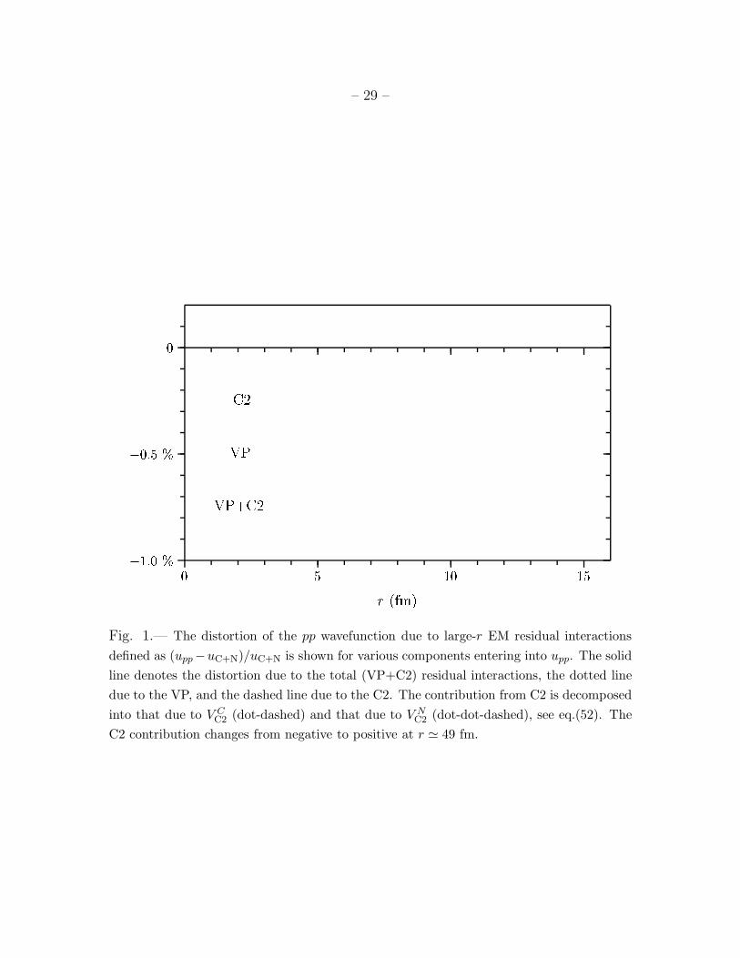
exhibited in Fig. 1, where we plot the ratio (upp − uC+N)/uC+N as a function of r.

– 17 –

5. Numerical Results

It is convenient to define the reduced matrix element of the weak current as

M ≡ M1B +M2B (53)

such that

〈ψd| ~J−|ψpp〉√8πgAASNpp

=

(

sd − iµV

2gAmN

~k × sd

)

M1B + sdM2B

=

(

sd − iµV

2gAmN

~k × sd

)

M+O(

Q4, Q2|~k|, |~k|2)

, (54)

where sd is the spin polarization vector of the deuteron and the normalization factors

AS and Npp have been defined in eqs.(26) and (49). Although the reshuffling of

terms in the last line introduces a term of O(Q3|~k|) (i.e., the product of the WM

term and two-body term), the error made thereby should be negligible. We give our

numerical results in the increasing orders in chiral counting.

5.1. O(1) & O(Q) contributions: The single-particle matrix element

It follows from eqs.(12) and (54) that the single-particle (reduced) matrix

element simplifies to

M1B =∫

∞

0dr ud(r)upp(r). (55)

Following the discussion given in the preceding section, we formally separate the

contributions into the “Coulomb plus nuclear part” and the “large-r part”

M1B = MC+N1B +M>

1B, (56)

MC+N1B ≡

∫

∞

0dr ud(r)uC+N(r), (57)

M>1B ≡

∫

∞

0dr ud(r) [upp(r)− uC+N(r)] . (58)

Clearly the most important term is the “Coulomb plus nuclear term” eq.(57),

so it needs to be calculated as accurately as possible. This term can in turn be

decomposed into a term which can be extracted from experiments using the effective

range formula and the remainder that requires theoretical input from the Argonne

potential:

MC+N1B = MER

1B + δMC+N1B . (59)

– 18 –

If the next-to-leading-order approximation is made to the effective range formula,

the resulting matrix element is

MER1B ≡

∫

∞

0dr φd(r)φC(r)

+1

2

∫

∞

0dr

{[

u2d(r) + w2d(r)

1 + η2d− φ2

d(r)

]

+[

u2C+N(r)− φ2C(r)

]

}

(60)

= − eζ

aCγ2

[

1 +aC

R

(

E1(ζ)−e−ζ

ζ

)]

− ρd + rC

4, (61)

where ζ ≡ (γR)−1 and

E1(ζ) =∫

∞

1dt

e−ζt

t=∫

∞

ζdt

e−t

t. (62)

Now we can evaluate MER1B with the experimental values for the low-energy constants

given in eqs.(27), (30) and (47). The result is

MER1B

∣

∣

∣

exp= 5.986(1) fm− 1.138(5) fm (63)

where we have given the individual contributions of the two terms in eq.(61). If one

calculates with the Argonne potential instead of using the experimental data, one

obtains

MER1B

∣

∣

∣

Argonne= 5.986 fm− 1.137 fm (64)

which shows once more that it is reasonable to identify the results given by the

Argonne potential with “experiments”. We can now estimate accurately the

remaining small contribution coming from the difference between eqs.(57) and (60)

using the Argonne wavefunctions:

δMC+N1B = 0.011 fm. (65)

Since this quantity is very small and the Argonne wavefunction is accurate enough,

we have not included the error associated with this correction. Combining eqs.(63)

and (65), we obtain

MC+N1B = (1∓ 0.02 %∓ 0.07 %∓ 0.02 %) · 4.859 fm, (66)

where the first error comes from the uncertainty in aC , the second from rC and the

third from ρd. (The use of “∓” instead of “±” indicates that MC+N1B decreases as

each of |aC |, rC and ρd increases.)

Finally the effects of the residual C2 and VP potentials are calculated from

eq.(58):

M>1B = MVP

1B +MC21B = −0.031 fm (67)

– 19 –

with MVP1B = −0.022 fm and MC2

1B = −0.009 fm. For later purpose, we evaluate the

ratio

δ1B ≡ M>1B

MC+N1B

= δVP1B + δC2

1B = −0.63 %, (68)

with

δVP1B = −0.45 %,

δC21B = δC2:C

1B + δC2:N1B = (0.03 %) + (−0.21 %) = −0.18 %, (69)

where we have presented each contribution from V CC2 and V N

C2. It is worth noting

that the contribution from the C2 potential is about 40 % of the VP contribution,

and has the same sign. This is contrary to what one would expect if the V NC2 were

ignored.

We follow KB (1994) and express the result obtained up to this point in terms

of Λ defined by

Λ ≡(

(aC)2γ3

2

)1

2

AS M1B. (70)

In terms of Λ, our result can be summarized as [see eq.(66)]#11

Λ2 = (1 + δ1B)2 (1± 0.01%∓ 0.07%± 0.07%)2 × 7.02, (71)

= (1± 0.01%∓ 0.07%± 0.07%)2 × 6.93 (72)

where again the errors correspond to the uncertainties in |aC |, rC and ρd (or AS)

in this order. The only possible sources of theoretical error, which are due to

uncertainties in the Argonne potential, are in δMC+N1B (eq.[65]) and δC2:N

1B (eq.[69]).

If we were to assign conservatively a ∼ 50% error to the two quantities there, the

resulting theoretical error on the reduced matrix element would then be ∼ 0.1 %.

5.2. Calculation of MC+N1B in effective field theory

In Section 2, we argued that the calculation of the single-particle matrix

element of the electroweak current using the Argonne wavefunctions is equivalent to

#11 If one calculates with the Argonne wavefunctions instead of using the experimental values, one

finds Λ2|Argonne = (1 + δ1B)2 × 7.03.

– 20 –

a “first-principle” calculation using effective field theory of QCD. How this comes out

in the case of the np capture was discussed in (Park et al. 1997b). Here we briefly

report the result of a first-principle calculation for the leading Gamow-Teller matrix

element eq.(57). Such a calculation involving the Coulomb potential is interesting

on its own merit, so we shall describe it in detail elsewhere (Park et al. 1998).

As in (Park et al. 1997b), we shall integrate out all fields other than the matter

field for the nucleon and treat to next-to-leading order (NLO). The potential has

then the contact interactions used for the np channel plus the Coulomb interaction

V (~q) =4π

mN

[

C0 + (C2δij +D2σ

ij)qiqj]

+ Z1Z2α

~q2,

σij =3√8

(

σi1σ

j2 + σj

1σi2

2− δij

3~σ1 · ~σ2

)

. (73)

In our case, of course, Z1Z2 = 1 for the pp channel and 0 for the np channel. Since

the Coulomb interaction is not separable, we use the Gaussian regulator as

V (~r) =∫ d3~q

(2π)3SΛ(~q

2) ei~q·~r V (~q) (74)

with

SΛ(~q2) = exp

(

− ~q2

2Λ2

)

(75)

where Λ is the cut-off. The coefficients C0,2 for the spin singlet and triplet channels

and D2 are fixed by np scattering and the properties of the deuteron. The cut-off Λ

defines a regime in which the effective theory is applicable. It is not a free parameter.

By the rule of (cut-off) effective field theory, physical quantities should not depend

sensitively on the exact form of the cut-off nor on the exact value of Λ. Since the

pion is integrated out, the cut-off should be ∼ mπ. Indeed as we found in (Park

et al. 1997b), all the static properties of the deuteron are well reproduced for the

range of cut-off, (140 ∼ 200) MeV.#12 For this range of cut-off, the one-body matrix

element for the np capture comes out to be 4.00 ∼ 3.96 which agrees well with the

result of the Argonne wavefunction (“experiment”), 3.98. The same formalism turns

out to give

MC+N1B (EFT) = 4.89 ∼ 4.85. (76)

#12 The numerical values of Λ figuring here could very well be slightly different from the value in

(Park et al. 1997b) because of the slightly different regularizations involved. The range of Λ found

there to give correct static properties of the deuteron was about (160 ∼ 220) MeV.

– 21 –

As in the case of the np capture, this agrees closely with what we might refer to

as the “experimental” value, 4.86, with an error of about 0.5 %. This validates

our assertion made in Section 2.#13 In our approach, the corrections from the V>

potential are found to be

δVP1B = −0.45 %, δC2:C

1B = 0.03 %, δC2:N1B = −(0.19 ∼ 0.15) %. (77)

These values validate the former calculation, eq.(69), where we used Argonne

wavefunction corresponding to the all order of contributions. Both δVP1B and δC2:C

1B

are found to be extremely insensitive to the cut-off. Even δC2:N1B turns out to be only

mildly dependent on Λ. This is somewhat surprising, for the effect of V NC2 ∝ 1

rVN(r)

is expected to be amplified at small r by the nuclear potential.

5.3. O(Q3) contribution: The exchange-current matrix element

The matrix element of the two-body current eq.(22) can be separated into

three pieces,

M2B = Mfinite2B +Mkin

2B +Mδ2B (78)

where Mkin2B is the contribution from the “kinetic term”, Mδ

2B is the zero-ranged

contributions, and Mfinite2B is the remaining finite-range contribution. From eqs.(54)

and (22)

Mfinite2B =

2

3

(

c3 + 2c4 +1

2

)

m3π

mNf 2π

∫

∞

0dr ud(r)y0(mπr)upp(r)

− 2√2

3

(

c3 − c4 −1

4

)

m3π

mNf 2π

∫

∞

0dr wd(r)y2(mπr)upp(r), (79)

Mkin2B =

m3π

3mNf 2π

∫

∞

0dry1(mπr)

2m2πr

[

ud(r)u′

pp(r)− u′d(r)upp(r)]

−√2m3

π

3mNf 2π

∫

∞

0dry1(mπr)

2m2πr

[

wd(r)u′

pp(r)− w′

d(r)upp(r)−3

rwd(r)upp(r)

]

,(80)

Mδ2B = −2

(

d1 − 2d2 +1

3c3 +

2

3c4 +

1

6

)

1

mNf 2π

∫

∞

0dr ud(r)

δ(r)

4πr2upp(r). (81)

#13 While small in magnitude from the view point of the next-to-leading order EFT, the error bar

of about 0.5 % is bigger than that with the Argonne potential, ∼ 0.1 %. This difference may be

accounted for by the next-order contribution, namely, the effective volume term, which we have not

considered.

– 22 –

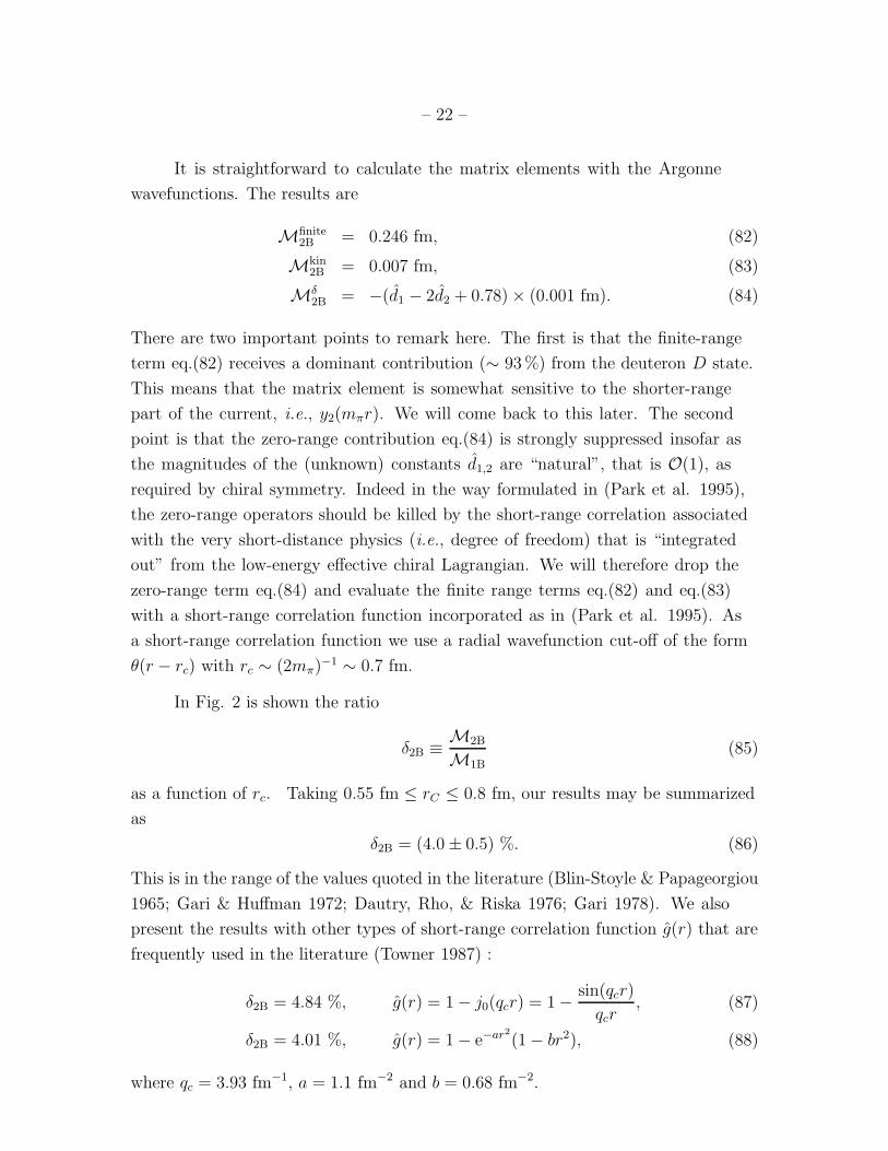
It is straightforward to calculate the matrix elements with the Argonne

wavefunctions. The results are

Mfinite2B = 0.246 fm, (82)

Mkin2B = 0.007 fm, (83)

Mδ2B = −(d1 − 2d2 + 0.78)× (0.001 fm). (84)

There are two important points to remark here. The first is that the finite-range

term eq.(82) receives a dominant contribution (∼ 93%) from the deuteron D state.

This means that the matrix element is somewhat sensitive to the shorter-range

part of the current, i.e., y2(mπr). We will come back to this later. The second

point is that the zero-range contribution eq.(84) is strongly suppressed insofar as

the magnitudes of the (unknown) constants d1,2 are “natural”, that is O(1), as

required by chiral symmetry. Indeed in the way formulated in (Park et al. 1995),

the zero-range operators should be killed by the short-range correlation associated

with the very short-distance physics (i.e., degree of freedom) that is “integrated

out” from the low-energy effective chiral Lagrangian. We will therefore drop the

zero-range term eq.(84) and evaluate the finite range terms eq.(82) and eq.(83)

with a short-range correlation function incorporated as in (Park et al. 1995). As

a short-range correlation function we use a radial wavefunction cut-off of the form

θ(r − rc) with rc ∼ (2mπ)−1 ∼ 0.7 fm.

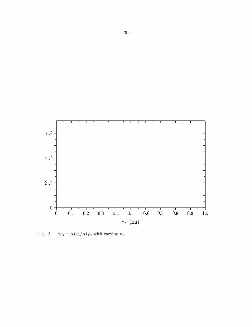
In Fig. 2 is shown the ratio

δ2B ≡ M2B

M1B(85)

as a function of rc. Taking 0.55 fm ≤ rC ≤ 0.8 fm, our results may be summarized

as

δ2B = (4.0± 0.5) %. (86)

This is in the range of the values quoted in the literature (Blin-Stoyle & Papageorgiou

1965; Gari & Huffman 1972; Dautry, Rho, & Riska 1976; Gari 1978). We also

present the results with other types of short-range correlation function g(r) that are

frequently used in the literature (Towner 1987) :

δ2B = 4.84 %, g(r) = 1− j0(qcr) = 1− sin(qcr)

qcr, (87)

δ2B = 4.01 %, g(r) = 1− e−ar2(1− br2), (88)

where qc = 3.93 fm−1, a = 1.1 fm−2 and b = 0.68 fm−2.

– 23 –

As mentioned, the non-negligible rC dependence in the region rC ∼> (2mπ)−1

comes from the fact that a short-range (or high-order) current and the D-state

component of the deuteron wavefunction are involved. This is due to the fact

that because of the symmetry involved, O(Q) and O(Q2) terms relative to the

single-particle operator are suppressed, an aspect closely related to the chiral

filter mechanism. This means that some terms higher order than the O(Q3) ones

calculated here – starting at O(Q4) and probing shorter length scales – may not be

negligible compared with the terms that are retained.#14

5.4. Cross section

For comparison with KB (1994), we focus on the low-energy cross-section

factor Spp(E) (Bahcall and May 1969),

Spp(E) ≡ σ(E)Ee2πη (89)

where σ(E) is the cross section for the process (1) and η = mpα

2p. Explicitly, it is of

the form

Spp(E) = (1 + δ2B)2 6

πmpαG

2V g

2A

Λ2

γ3m5

ef(E0 + E), (90)

where f(E0 +E) with E0 ≡ 2mp −md is the phase volume defined in (Bahcall 1966)

with however the WM term contribution as well as the deuteron recoil taken into

account. These two effects turn out to be very small.#15 Setting E ≈ 0, we have

SχPTpp (0) = 4.05

(

1 + δ2B1.04

)2 (gA

1.2601

)2(

Λ2

6.93

)

× (10−25 MeV-barn) (91)

where we have substituted GV = 1.1356 × 10−5 GeV−2 and the phase volume

f(E0) = 0.1421. It is worth noting, in passing, that our result for the above S-factor

#14 For instance, if one adopts a phenomenological approach and calculates ρ-meson-exchange

diagrams involving a ρN∆ vertex (with form factors appended to all the vertices), the one-pion-

exchange contribution is found to be considerably quenched (Bargholtz 1979; Carlson et al. 1991).

From the chiral perturbation point of view, however, these diagrams come at O(Q4) or higher, and

therefore they need to be calculated together with all other diagrams of the same chiral order. We

will not attempt such a calculation here.

#15 The WM term increases f by 0.02 % while the deuteron recoil correction decreases it by 0.06 %,

so the net effect is a 0.04 % decrease.

– 24 –

is a precise prediction based upon the Standard Model, that is, without neutrino

mass (oscillation). The corresponding expression given by KB (1994) is

SKBpp (0) = 3.89

(

1 + δ2B1.01

)2 (gA

1.2573

)2(

Λ2

6.92

)

× (10−25 MeV-barn). (92)

By plugging in the numbers obtained above, we arrive at

SχPTpp (0) = 4.05 × 10−25(1± 0.15 %± 0.48 %)2 MeV-barn (93)

where the first error arises from the one-body matrix element and the second from

the two-body term due to the uncertainty in the short-range correlation. (The latter

does not include the possible contribution of the next order (i.e., O(Q4)) term; see

later.) This is to be compared with that of KB

SKBpp (0) = 3.89 × 10−25(1± 1.1 %)MeV-barn. (94)

We are now ready to make a detailed comparison between our result and that

of KB:

1. The weak-interaction constants used by KB are: gA = 1.2575 and

GV = 1.151 × 10−5 GeV−2 (Freedman 1990)#16. Ours are gA = 1.2601 and

GV = 1.136× 10−5 GeV−2.

2. KB gave Λ2 = 6.92 and δ2B = 1 % while we have obtained Λ2 = 6.93 and

δ2B = 4 %.

Apart from small differences in the constants used, the major difference is in the

exchange-current contribution. In the next section, we will discuss whether this is

a genuine difference and to what extent our calculation will be affected by higher

chiral-order terms.

Although, as noted by KB (1994), the corrections due to the long-range

potential V> are small, it may be of some interest to make a few remarks on its

role. Our result is that the VP potential decreases the pp rate by about 0.9 % in

agreement with (Bohannon & Heller 1977) (where the decrease was found to be

about 0.8 ∼ 1.2 %) as well as with KB (1994), who found a 0.9 % decrease#17. Our

#16 The value of GV is not given explicitly in KB (1994), but we can reproduce eq.(94) only with

the use of this value of GV , a value which was also adopted in (Carlson 1991).

#17 As mentioned, despite the similarity in the numerical results, our calculational framework is

different from that of KB. This difference will be analyzed in detail elsewhere (Park et al. 1998).

– 25 –

result is slightly at variance with that of (Gould 1990), wherein with the use of

the WKB approximation a 1.3 % decrease was found. In addition the C2 potential

lowers the pp rate by about 0.4 %. In total, therefore, the downward correction due

to V> is somewhat larger than that of KB. Since the Λ2 is about the same, this

means that our single-particle matrix element M1B is somewhat larger than that of

KB.

6. Discussion

Following the procedure of chiral perturbation theory proven to be highly

successful for the thermal np capture process, we have calculated the pp fusion rate

to O(Q3) in chiral counting relative to the leading single-particle Gamow-Teller

matrix element. To the order considered, the error involved in the calculation is

small, ∼< 1 %. This result, given a justification from a cut-off effective field theory of

low-energy QCD as in the case of the np capture (Park et al. 1997b), supports the

canonical value of Bahcall et al. and does not support the “relativistic field theory

model” result of Ivanov et al. (1997).

The main caveat in this calculation is in the meson-exchange contribution

which comes out to be about 4 % when calculated to the chiral order O(Q3). At

the next order, O(Q4), loops and higher-order counter terms enter, so that there

is no reason to believe that they are negligible compared with the O(Q3) tree

contributions. (For instance, it could be lowered to about 1 ∼ 2 % instead of ∼ 4 %

found here). This aspect is different from the case of the np capture where the chiral

filter mechanism assures the dominance of the tree-order pion exchange-current

contribution. Here the absence of the chiral filter phenomenon can allow higher-order

(loop) terms to figure equally importantly as the tree-order terms. From this

viewpoint it is not surprising that a model calculation of the terms of O(Q4) and

higher based on the vector-meson exchange and form factors (Bargholtz 1979)

indicates that there can be a considerable suppression of the tree-order correction.

Although such a reduction in the exchange-current contribution seems to go in the

right direction for beta decays of higher-mass nuclei (Carlson 1991), it is probably

unsafe to import the result of such model calculations into our work. To go to O(Q4)

or above in our theory at which heavy mesons and form factors come in, a large

number of Feynman graphs of the same chiral order have to be computed on the

same footing to assure chiral symmetry, and such a calculation has not been done

yet. In the absence of consistent calculations, our attitude is that we should not

– 26 –

attach any error estimates on terms not accounted for to the chiral order computed.

Calculating the higher-order terms will be left for a future exercise.

We are grateful to John Bahcall and Gerry Brown for stressing to us the need

to revisit this long-standing problem. MR is grateful to Chung Wook Kim, Director

of the Korea Institute for Advanced Study, for the invitation to the Institute, where

part of this paper was written. TSP is indebted to Francisco Fernandez for the

hospitality at Grupo de Fısica Nuclear, Universidad de Salamanca, where this work

was completed. The work of TSP and DPM was supported in part by the Korea

Science and Engineering Foundation through CTP of SNU and in part by the

Korea Ministry of Education under the grant BSRI-97-2418. The work of KK was

supported in part by NSF Grant No. PHYS-9602000.

REFERENCES

Bahcall, J. N. 1966, Nucl. Phys., 75, 10

Bahcall, J. N. 1997, in Unsolved Problems in Astrophysics, eds. Bahcall, J. N., &

Ostriker J. P. (Princeton: Princeton University Press)

Bahcall, J. N., & Kamionkowski, M. 1997, Nucl. Phys. A, 625, 893

Bahcall, J. N., & May, R. 1969, ApJ, 155, 501

Bargholtz, C. 1979, ApJ, 233, L161

Beane, S. R., Cohen, T. D., & Phillips, D. R. 1997, preprint [nucl-th/9709062] and

references therein

Bergervoet, J. R., van Campen, P. C., van der Sanden, W. A., & de Swart, J. J.

1988, Phys. Rev. C, 38, 15

Bernard, V., Kaiser, N., & Meissner, Ulf-G. 1997, Nucl. Phys. A, 615, 483

Bethe, H., & Critchfield, C. L. 1938, Phys. Rev., 54, 248

Blin-Stoyle, R. J., & Papageorgiou, S. 1965, Nucl. Phys., 64, 1

Bohannon, G. E., & Heller, L. 1977, Phys. Rev. C, 38, 1221

Carlson, J., Riska, D. O., Schiavilla, R., & Wiringa, R. B. 1991, Phys. Rev. C, 44,

619

– 27 –

Cohen, T. D., Friar, J. L., Miller, G. A., & van Kolck, U. 1996, Phys. Rev. C, 53,

2661

Dautry, F., Rho, M., & Riska, D. O. 1976, Nucl. Phys. A, 264, 507

Degl’Innocenti, S., Fiorentini, G., & Ricci, B. 1998, Phys. Lett. B, 416, 365

Ericson, T. E. O., & Rosa-Clot, M. 1983, Nucl. Phys. A, 405, 497

Freedman, S. 1990, Comments Nucl. Part. Phys., 19, 209

Gari, M. 1978, Proceedings of Informal Conference on Status and Future of Solar

Neutrino Research, Report No. 50879, Vol. 1, ed. G. Friedlander (Upton:

Brookhaven National Laboratory), 137

Gari, M., & Huffman, A. H. 1972, ApJ, 178, 543

Gould, R. J. 1990, ApJ, 359, L67

Ivanov, A. N., Troitskaya, N. I., Faber, M., & Oberhummer, H. 1997, Nucl. Phys. A,

617, 414; Erratum-ibid.A618, 509; Erratum-ibid.A625, 896; Oberhummer,

H., Ivanov, A. N., Troitskaya, N. I., & Faber, M. 1997, preprint [astro-

ph/9705119]

Kamionkowski, M., & Bahcall, J. N. 1994, ApJ, 420, 884

Kaplan, D. B., Savage, M. J., & Wise, M. B. 1996, Nucl. Phys. B, 478, 629; preprint

[nucl-th/9802075]

van der Leun, C., & Alderliesten, C. 1982, Nucl. Phys. A, 380, 261

Luke, M., & Manohar, A. V. 1997, Phys. Rev. D, 55, 4129

Ordonez, C., Ray, L., & van Kolck, U. 1994, Phys. Rev. Lett., 72, 1982; 1996,

Phys. Rev. C, 53, 2086

Park, T.-S., Min, D.-P., & Rho, M. 1993, Phys. Rep., 233, 341; Park, T.-S., Towner,

I. S., & Kubodera, K. 1994, Nucl. Phys. A, 579, 381

Park, T.-S., Min, D.-P., & Rho, M. 1995, Phys. Rev. Lett., 74, 4153; 1996,

Nucl. Phys. A, 596, 515

Park, T.-S., Jung, H., & Min, D.-P. 1997a, Phys. Lett. B, 409, 26

– 28 –

Park, T.-S., Kubodera, K., Min, D.-P., & Rho, M. 1997b, Phys. Rev. Lett.,

submitted [hep-ph/9711463]

Park, T.-S., Kubodera, K., Min D.-P., & Rho, M. 1998, in preparation

(Particle Data Group July 1996 :) R.M. Barnett et al. 1996, Phys. Rev. D, 54, 1

Rho, M. 1991, Phys. Rev. Lett., 66, 1275

Rodning, N. L., & Knutson, L. D. 1990, Phys. Rev. C, 41, 898

Salpeter, E. E. 1952, Phys. Rev., 88, 547

Towner, I. S. 1987, Phys. Rep., 155, 263

Weinberg, S. 1990, Phys. Lett. B, 251, 288; 1991, Nucl. Phys. B, 363, 3; 1992, Phys.

Lett. B, 295, 114

Weinberg, S. 1996, The Quantum Theory of Fields II, (Cambridge: Cambridge

Press), 192; 1997, Nature, 386, 234

Wiringa, R. B., Stoks, V. G. J., & Schiavilla, R. 1995, Phys. Rev. C, 51, 38

This preprint was prepared with the AAS LATEX macros v4.0.

– 29 –

�1:0 %

�0:5 %

0

0 5 10 15

r (fm)

.

.

.

.

.

.

..

.

.

.

.

.

.

.

.

.

.

.

.

.

.

.

.

.

.

.

.

.

.

.

.

.

.

.

.

.

.

.

.

.

.

.

.

.

.

.

.

.

.

.

.

.

.

.

.

.

.

.

.

.

.

.

.

.

.

.

.

.

.

.

.

.

.

.

.

.

.

.

.

.

.

.

.

.

.

.

.

.

.

.

.

.

.

.

.

.

.

.

.

.

.

.

.

.

.

.

.

.

.

.

.

.

.

.

.

.

.

.

.

.

.

.

.

.

.

.

.

.

.

.

.

.

.

.

.

.

.

.

.

.

.

.

.

.

.

.

.

.

.

.

.

.

.

.

.

.

.

.

.

.

.

.

.

.

.

.

.

.

.

.

.

.

.

.

.

.

.

.

.

.

.

.

.

..

.

.

.

.

.

.

.

.

.

.

.

.

.

.

.

.

.

.

.

.

.

.

.

.

.

.

.

.

.

.

.

.

.

.

.

.

.

.

.

.

.

.

.

.

.

.

.

.

.

.

.

.

.

.

.

.

.

.

.

.

.

.

.

.

.

.

.

.

.

.

.

.

.

.

.

.

.

.

.

.

.

.

.

.

.

.

.

.

.

.

.

.

.

.

.

.

.

.

.

.

.

.

.

.

.

.

.

.

.

.

.

.

.

.

.

..

.

.

.

.

.

.

.

.

.

.

.

.

.

.

.

.

.

.

.

.

.

.

.

.

.

.

.

.

.

.

.

.

.

.

.

.

.

.

.

.

.

.

.

.

.

.

.

.

.

.

.

.

.

.

.

.

.

.

.

.

.

.

.

.

.

.

.

.

.

.

.

..

.

.

.

.

.

.

.

.

.

.

.

.

.

.

.

.

.

.

.

.

.

.

.

.

.

.

.

.

.

.

.

.

.

.

.

.

.

.

.

.

.

.

.

..

.

.

.

.

.

.

.

.

.

.

.

.

.

.

.

.

.

.

.

.

.

.

.

.

.

.

..

.

.

.

.

.

.

.

.

.

.

.

.

.

.

.

..

.

.

.

.

.

.

.

.

..

.

.

.

.

.

..

.....................

.

.

.

.

.

.

.

.

.

.

.

.

..

.

.

.

.

.

.

.

.

.

.

.

.

.

..

.

.

.

.

.

.

.

.

.

.

.

.

.

..

.

.

.

.

.

.

.

.

.

.

.

.

.

..

.

.

.

.

.

.

.

.

.

.

.

.

.

..

.

.

.

.

.

.

.

.

.

.

.

.

.

..

.

.

.

.

.

.

.

.

.

.

.

.

.

..

.

.

.

.

.

.

.

.

.

.

.

.

.

..

.

.

.

.

.

.

.

.

.

.

.

.

.

..

.

.

.

.

.

.

.

.

.

.

.

.

.

..

.

.

.

.

.

.

.

.

.

.

.

.

.

..

.

.

.

.

.

.

.

.

.

.

.

.

.

.

.

.

.

.

.

.

.

.

.

.

.

.

.

..

.

.

.

.

.

.

.

.

.

.

.

.

.

.

.

.

.

.

.

.

.

.

.

.

.

.

.

..

.

.

.

.

.

.

.

.

.

.

.

.

.

.

.

.

.

.

.

.

.

.

.

.

.

.

.

..

.

.

.

.

.

.

.

.

.

.

.

.

.

.

.

.

.

.

.

.

.

.

.

.

.

.

.

..

.

.

.

.

.

.

.

.

.

.

.

.

.

.

.

.

.

.

.

.

.

.

.

.

.

.

.

..

.

.

.

.

.

.

.

.

.

.

.

.

.

.

.

.

.

.

.

.

.

.

.

.

.

.

.

..

.

.

.

.

.

.

.

.

.

.

.

.

.

.

.

.

.

.

.

.

.

.

.

.

.

.

..

...................................................................................................................................................................................................................................................................................................................................................................................................................................................................................

VP+C2

.

.

.

.

.

.

.

.

.

.

.

.

.

.

.

.

.

.

.

.

.

.

.

.

.

.

.

.

.

.

.

.

.

.

.

.

.

.

.

.

.

.

.

.

.

.

.

.

.

.

.

.

.

.

.

.

.

.

.

.

.

.

.

.

.

.

.

.

.

VP

.

.

.

.

.

.

.

.

.

.

.

.

.

.

.

.

.

.

.

.

.

.

.

.

.

.

.

.

.

.

.

.

.

.

.

.

.

.

.

.

.

.

.

.

.

.

.

.

.

.

.

.

.

.

.

.

.

.

.

.

.

.

.

.

.

.

.

.

.

.

.

.

.

.

.

.

.

.

.

.

.

.

.

.

.

.

.

.

.

.

.

.

.

.

.

.

.

.

.

.

.

.

.

.

.

.

.

.

.

.

.

.

.

.

.

.

.

.

.

.

.

.

.

.

.............

.

.

.

.

.

.

.

.

.

.

.

.

.

.

.

.

.

.

.

.

.

.

.

.

.

.

.

.

.

.

.

.

.

.

.

.

.

.

.

.

.

.

.

.

.

.

.

.

.

.

.

.

.

.

.

.

.

.

.

.

.

.

.

.

.

.

.

.

..

.

.

.

.

.

.

.

.

.

.

.

.

..

.

.

.

.

...

.

.

..

.

.

..

.

.

.

..

.

.

.

..

.

..

.

.

..

.

.

.

..

.

..

.

.....

..

.

..........

.

..

.

.........

.

............

.

............

.............

.............

.............

.

............

.

............

.............

.............

..

...........

.............

.

............

.............

.............

.............

.............

.............

.............

.............

.............

C2

.

.

.

......................................................................................................................................................................................................................................................................................................................................................................................

................................

................................................................

....................................................

..........................................................

.

.

.

.

.

.

.

.

.

.

.

.

.

.

.

.

.

.

.

.

.

.

.

.

.

.

.

.

.

.

.

.

.

.

.

.

.

.

.

.

.

.

.

.

.

.

.

.

.

.

.

.

.

.

.

.

.

.

.

.

.

.

.

.

.

.

.

.

.

.

.

.

.

.

.

.

.

.

.

.

.

.

.

.

.

.

.

.

.

.

.

.

.

.

.

.

.

.

.

.

.

.

.

.

.

.

.

.

.

.

.

.

.

.

.

.

.

.

.

.

.

.

.

.

.

.

.

.

.

.

.

.

.

.

.

.

.

.

.

.

.

.

.

.

.

.

.

.

.

.

.

.

.

.

.

.

.

...

.

..

.

.

.

.

.

.

.

.

.

.

.

.

.

.

.

.

.

.

.

.

.

.

.

.

.

.

.

.

.

.

.

.

.

.

.

.

.

.

.

.

.

.

.

.

.

.

.

.

.

.

.

.

.

.

.

.

.

.

.

.

.

.

.

.

.

.

.

.

.

.

.

.

.

.

.

.

.

.

.

.

.

.

.

.

.

.

.

.

.

.

.

.

.

.

.

.

..........................

...

.

.

.

.

.

.

.

......................

.

.

.

..

.

..........................

.

..

.

..

.

.

........................

..

.

.

..

.

..

.......................

.

..

...

.

.........................

...

...

..........................

...

...

..........................

..

.

..

.

..........................

...

...

..

........................

...

................................................................

...

..............

Fig. 1.— The distortion of the pp wavefunction due to large-r EM residual interactions

defined as (upp−uC+N)/uC+N is shown for various components entering into upp. The solid

line denotes the distortion due to the total (VP+C2) residual interactions, the dotted line

due to the VP, and the dashed line due to the C2. The contribution from C2 is decomposed

into that due to V CC2 (dot-dashed) and that due to V N

C2 (dot-dot-dashed), see eq.(52). The

C2 contribution changes from negative to positive at r ≃ 49 fm.

– 30 –

0

2 %

4 %

6 %

0 0:1 0:2 0:3 0:4 0:5 0:6 0:7 0:8 0:9 1:0

r

C

(fm)

...................................................................

..........................................................................................................................................................................................................................................................................................................................................................................................................................................................

.

.

.

.

.

.

.

.

.

.

.

.

.

.

.

.

.

.

.

.

..

.

.

.

.

.

.

.

.

.

.

.

.

.

.

.

.

.

.

.

.

.

..

.

.

.

.

.

.

.

.

.

.

.

.

.

.

.

.

.

.

.

.

.

..

.

.

.

.

.

.

.

.

.

.

.

.

.

.

.

.

.

.

.

.

.

..

.

.

.

.

.

.

.

.

.

.

.

.

.

.

.

.

.

.

.

.

.

..

.

.

.

.

.

.

.

.

.

.

.

.

.

.

.

.

.

.

.

.

.

..

.

.

.

.

.

.

.

.

.

.

.

.

.

.

.

.

.

.

.

.

.

.

..

.

.

.

.

.

.

.

.

.

.

.

.

.

.

.

.

.

.

.

.

.

.

..

.

.

.

.

.

.

.

.

.

.

.

.

.

.

.

.

.

.

.

.

.

.

..

.

.

.

.

.

.

.

.

.

.

.

.

.

.

.

.

.

.

.

.

.

.

..

.

.

.

.

.

.

.

.

.

.

.

.

.

.

.

.

.

.

.

.

.

.

..

.

.

.

.

.

.

.

.

.

.

.

.

.

.

.

.

.

.

.

.

.

.

..

.

.

.

.

.

.

.

.

.

.

.

.

.

.

.

.

.

.

.

.

.

.

..

.

.

.

.

.

.

.

.

.

.

.

.

.

.

.

.

.

.

.

.

.

..

.

.

.

.

.

.

.

.

.

.

.

.

.

.

.

.

.

.

.

.

.

..

.

.

.

.

.

.

.

.

.

.

.

.

.

.

.

.

.

.

.

.

.

..

.

.

.

.

.

.

.

.

.

.

.

.

.

.

.

.

.

.

.

.

.

.

Fig. 2.— δ2B ≡ M2B/M1B with varying rC .