arX

iv:q

-alg

/960

1002

v2 1

6 Ja

n 19

96

AN INVARIANT OF INTEGRAL HOMOLOGY 3-SPHERES

WHICH IS UNIVERSAL FOR ALL FINITE TYPE INVARIANTS

THANG T. Q. LE

Abstract. In [LMO] a 3-manifold invariant Ω(M) is constructed using a modificationof the Kontsevich integral and the Kirby calculus. The invariant Ω takes values in agraded Hopf algebra of Feynman 3-valent graphs. Here we show that for homology 3-spheres the invariant Ω is universal for all finite type invariants, i.e. Ωn is an invariantof order 3n which dominates all other invariants of the same order. This shows thatthe set of finite type invariants of homology 3-spheres is equivalent to the Hopf algebraof Feynman 3-valent graphs. Some corollaries are discussed. A theory of groups ofhomology 3-spheres, similar to Gusarov’s theory for knots, is presented.

1. Introduction

In a previous work [LMO] (joint with J. Murakami and T. Ohtsuki) we defined a 3-manifold invariant Ω with values in, as expected in perturbative Chern-Simon theory (see[AS1, AS2, Ko2, Roz, Wit]), the graded Hopf algebra D of vertex-oriented 3-valent graphs.The construction uses a modification of the Kontsevich integral and the Kirby calculus.Actually, Ω corresponds only to the trivial connection in the perturbation theory. Onecan expect that Ω plays an important role in the set of homology 3-sphere invariants.

The first non-trivial degree part Ω1 is essentially the Casson invariant; and Ω canbe regarded as a far generalization of the Casson invariant. The degree n part of Ω isconstructed using finite type invariants of links of order ≤ (l +1)n, where l is the numberof components of the link.

Finite type invariants for knots and links were introduced by Vassiliev, see [Vas, BL],and proved to be very useful in knot theory. Kontsevich [Ko1] introduced a knot invariant,called the Kontsevich integral, with values in a graded algebra of chord diagrams. Thegrading n part of the Kontsevich integral is a finite type invariant of order n; and it isuniversal, since it dominates all other invariants of the same order. All quantum invariants,including the Jones polynomial, are special values of the Kontsevich integral, obtainedusing weight systems coming from semi-simple Lie algebras (see Theorem 10 of [LM2] andTheorem XX.8.3 of [Kas]).

Using sl2 quantum invariants at roots of unity, Reshetikhin and Turaev [RT] constructedquantum invariants of 3-manifolds. There are generalizations for other quantum groups.The algebraic part of the construction is the complicated theory of modular Hopf algebraand quantum groups at roots of unity, see [Tur].

Since quantum invariants of links are special values of the Kontsevich integral, therearose a question of constructing 3-manifold invariants from the Kontsevich integral. In[LMO], we succeeded in constructing such an invariant Ω. Actually we used a modificationof the Kontsevich integral, called the universal Kontsevich-Vassiliev invariant for framedlinks and tangles (see [LM1, LM2]).

1

2 THANG T. Q. LE

Invariants of finite type for homology 3-spheres were introduced by Ohtsuki [Oh1], inanalogy with the knot case. The theory was developed further in [GL1, GL2, GO1, GO2,Hab, Lin] and others. In particular, it was proved that orders of finite type invariantsare multiples of 3 (see [GL1, GO1]), and that the space of invariants of a fixed order isfinite-dimensional (see [Oh1]).

Both finite type invariants for links and for homology 3-spheres can be considered as away to organize the set of invariants in a systematical way. While a lot has been knownabout the knot case, much less is for the manifold case.

The aim of this paper is to show that for homology 3-spheres, Ω is as powerful as the setof all finite type invariants; i.e. Ω is a counterpart of the Kontsevich integral in knot theory.We show that the degree n part of Ω is an invariant of degree 3n which dominates all otherinvariants of degree 3n. This implies that the set of finite type invariants of homology3-spheres is equivalent to the (purely combinatorial) Hopf algebra D of Feynman 3-valentdiagrams. For example, the number of linearly independent invariants of degree ≤ n isequal the number of linearly independent 3-valent diagrams of degree ≤ n. The study offinite type invariants of homology 3-spheres is reduced to the study of Ω.

The proof of the main theorem is much more complicated than that of the similartheorem in the knot case. We have to use many results of the theory of the (modified)Kontsevich integral. We show that every weight system, defined in [GO1], can be in-tegrated to a finite type invariant, like in the knot case (and hence give an affirmativeanswer to Question 1 there).

We also show that for every n, there is a homology 3-sphere M which cannot bedistinguished from S3 by any invariant of order < 3n, but can be distinguished from S3

by an invariant of order 3n. An operation on homology 3-spheres which does not altervalues of invariants of order less than a fixed number is presented. A theory of groupsof homology 3-spheres, similar to Gusarov’s groups of knots, is sketched. Some othercorollaries of the main theorem are presented.

The paper is organized as follows. In Sections 2 we recall the universal Kontsevich-Vassiliev invariant for framed oriented links and tangles, considered in [LM1, LM2]. Wealso show some properties of this invariant, needed later. In Section 3 we give a definitionof Ω, and recall some fundamental concepts in the theory of finite type invariants ofhomology 3-spheres. In Section 4 we present the main results and discuss some corollariesand related problems. In Section 5 we prove the lemmas needed in the proof of the maintheorem.

The author would like to thank W. Menasco, J. Murakami and T. Ohtsuki for usefuldiscussions.

2. Chord diagrams and finite type invariants for framed tangles

2.1. Chord diagrams. Note that our definition of chord diagrams is more general thanthat of [BN1, LM1, LM2]. All vector spaces are over the field Q of rational numbers.

A uni-trivalent graph is a graph every vertex of which is either univalent or trivalent.A uni-trivalent graph is vertex-oriented if at each trivalent vertex a cyclic order of edgesis fixed. A 3-valent (resp. 1-valent) vertex is called an internal (external) vertex.

Let X be a compact oriented 1-dimensional manifold whose components are num-bered. A chord diagram with support X is the manifold X together with a vertex-oriented

A UNIVERSAL INVARIANT OF HOMOLOGY 3-SPHERES 3

uni-trivalent graph whose external vertices are on X; and the graph does not have anyconnected component homeomorphic to a circle.

In figures components of X are depicted by solid lines, while the graph is depicted bydashed lines, with the convention that the orientation at every vertex is counterclockwise.Each chord diagram has a natural topology. Two chord diagrams ξ, ξ′ on X are regardedas equal if there is a homeomorphism f : ξ → ξ′ such that f |X is a homeomorphism of Xwhich preserves components and orientation and the restriction of f to the dashed graphis a homeomorphism preserving orientation at every vertex.

There may be connected components of the dashed graph which do not have univalentvertices, and hence do not connect to any solid lines.

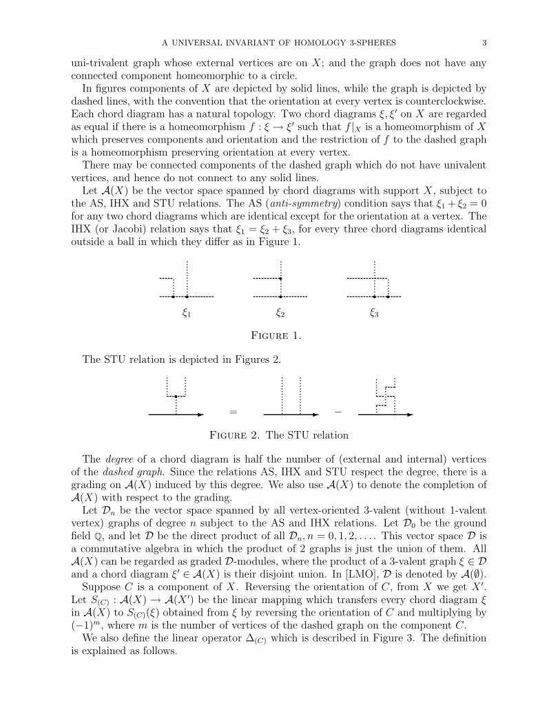
Let A(X) be the vector space spanned by chord diagrams with support X, subject tothe AS, IHX and STU relations. The AS (anti-symmetry) condition says that ξ1 + ξ2 = 0for any two chord diagrams which are identical except for the orientation at a vertex. TheIHX (or Jacobi) relation says that ξ1 = ξ2 + ξ3, for every three chord diagrams identicaloutside a ball in which they differ as in Figure 1.

ξ1

r rξ2

rrξ3

r rFigure 1.

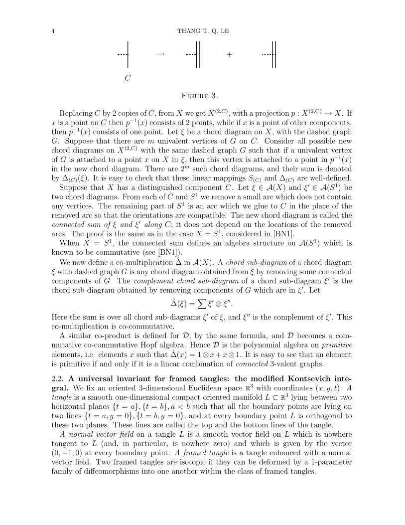
The STU relation is depicted in Figures 2.

r- = - − -

Figure 2. The STU relation

The degree of a chord diagram is half the number of (external and internal) verticesof the dashed graph. Since the relations AS, IHX and STU respect the degree, there is agrading on A(X) induced by this degree. We also use A(X) to denote the completion ofA(X) with respect to the grading.

Let Dn be the vector space spanned by all vertex-oriented 3-valent (without 1-valentvertex) graphs of degree n subject to the AS and IHX relations. Let D0 be the groundfield Q, and let D be the direct product of all Dn, n = 0, 1, 2, . . . . This vector space D isa commutative algebra in which the product of 2 graphs is just the union of them. AllA(X) can be regarded as graded D-modules, where the product of a 3-valent graph ξ ∈ Dand a chord diagram ξ′ ∈ A(X) is their disjoint union. In [LMO], D is denoted by A(∅).

Suppose C is a component of X. Reversing the orientation of C, from X we get X ′.Let S(C) : A(X) → A(X ′) be the linear mapping which transfers every chord diagram ξin A(X) to S(C)(ξ) obtained from ξ by reversing the orientation of C and multiplying by(−1)m, where m is the number of vertices of the dashed graph on the component C.

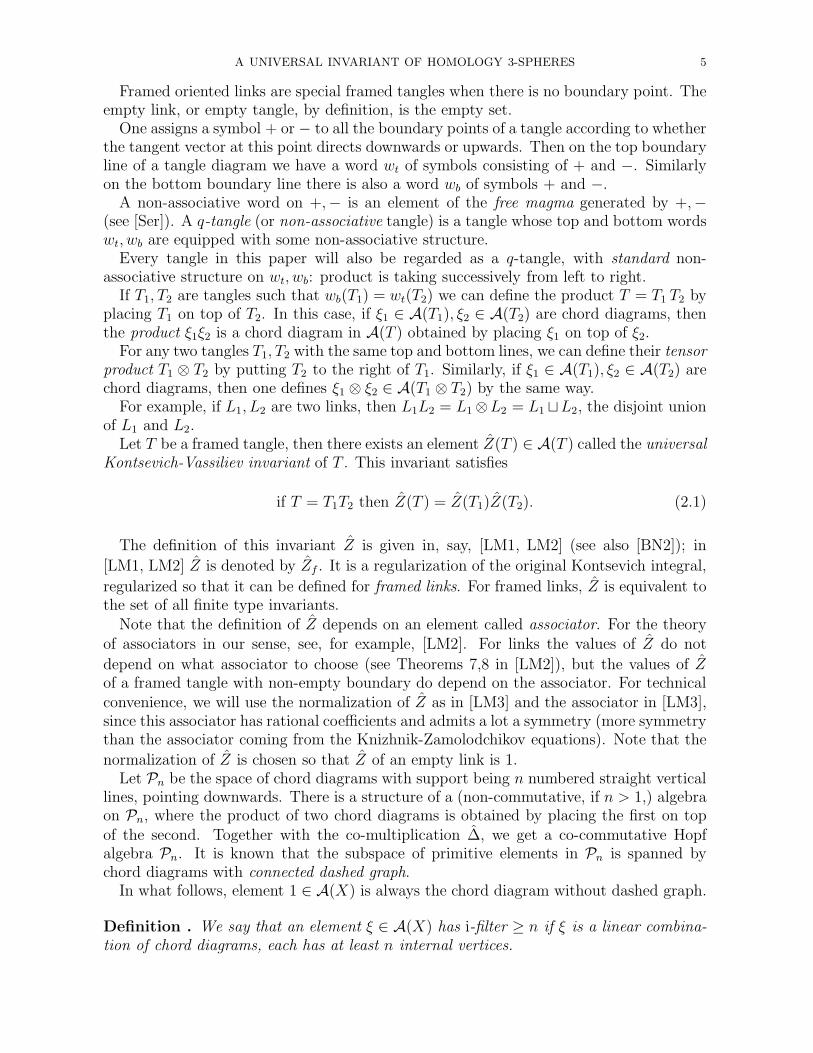
We also define the linear operator ∆(C) which is described in Figure 3. The definitionis explained as follows.

4 THANG T. Q. LE

C

→ +

Figure 3.

Replacing C by 2 copies of C, from X we get X(2,C), with a projection p : X(2,C) → X. Ifx is a point on C then p−1(x) consists of 2 points, while if x is a point of other components,then p−1(x) consists of one point. Let ξ be a chord diagram on X, with the dashed graphG. Suppose that there are m univalent vertices of G on C. Consider all possible newchord diagrams on X(2,C) with the same dashed graph G such that if a univalent vertexof G is attached to a point x on X in ξ, then this vertex is attached to a point in p−1(x)in the new chord diagram. There are 2m such chord diagrams, and their sum is denotedby ∆(C)(ξ). It is easy to check that these linear mappings S(C) and ∆(C) are well-defined.

Suppose that X has a distinguished component C. Let ξ ∈ A(X) and ξ′ ∈ A(S1) betwo chord diagrams. From each of C and S1 we remove a small arc which does not containany vertices. The remaining part of S1 is an arc which we glue to C in the place of theremoved arc so that the orientations are compatible. The new chord diagram is called theconnected sum of ξ and ξ′ along C; it does not depend on the locations of the removedarcs. The proof is the same as in the case X = S1, considered in [BN1].

When X = S1, the connected sum defines an algebra structure on A(S1) which isknown to be commutative (see [BN1]).

We now define a co-multiplication ∆ in A(X). A chord sub-diagram of a chord diagramξ with dashed graph G is any chord diagram obtained from ξ by removing some connectedcomponents of G. The complement chord sub-diagram of a chord sub-diagram ξ′ is thechord sub-diagram obtained by removing components of G which are in ξ′. Let

∆(ξ) =∑

ξ′ ⊗ ξ′′.

Here the sum is over all chord sub-diagrams ξ′ of ξ, and ξ′′ is the complement of ξ′. Thisco-multiplication is co-commutative.

A similar co-product is defined for D, by the same formula, and D becomes a com-mutative co-commutative Hopf algebra. Hence D is the polynomial algebra on primitiveelements, i.e. elements x such that ∆(x) = 1⊗x+x⊗1. It is easy to see that an elementis primitive if and only if it is a linear combination of connected 3-valent graphs.

2.2. A universal invariant for framed tangles: the modified Kontsevich inte-

gral. We fix an oriented 3-dimensional Euclidean space R3 with coordinates (x, y, t). A

tangle is a smooth one-dimensional compact oriented manifold L ⊂ R3 lying between twohorizontal planes t = a, t = b, a < b such that all the boundary points are lying ontwo lines t = a, y = 0, t = b, y = 0, and at every boundary point L is orthogonal tothese two planes. These lines are called the top and the bottom lines of the tangle.

A normal vector field on a tangle L is a smooth vector field on L which is nowheretangent to L (and, in particular, is nowhere zero) and which is given by the vector(0,−1, 0) at every boundary point. A framed tangle is a tangle enhanced with a normalvector field. Two framed tangles are isotopic if they can be deformed by a 1-parameterfamily of diffeomorphisms into one another within the class of framed tangles.

A UNIVERSAL INVARIANT OF HOMOLOGY 3-SPHERES 5

Framed oriented links are special framed tangles when there is no boundary point. Theempty link, or empty tangle, by definition, is the empty set.

One assigns a symbol + or − to all the boundary points of a tangle according to whetherthe tangent vector at this point directs downwards or upwards. Then on the top boundaryline of a tangle diagram we have a word wt of symbols consisting of + and −. Similarlyon the bottom boundary line there is also a word wb of symbols + and −.

A non-associative word on +,− is an element of the free magma generated by +,−(see [Ser]). A q-tangle (or non-associative tangle) is a tangle whose top and bottom wordswt, wb are equipped with some non-associative structure.

Every tangle in this paper will also be regarded as a q-tangle, with standard non-associative structure on wt, wb: product is taking successively from left to right.

If T1, T2 are tangles such that wb(T1) = wt(T2) we can define the product T = T1 T2 byplacing T1 on top of T2. In this case, if ξ1 ∈ A(T1), ξ2 ∈ A(T2) are chord diagrams, thenthe product ξ1ξ2 is a chord diagram in A(T ) obtained by placing ξ1 on top of ξ2.

For any two tangles T1, T2 with the same top and bottom lines, we can define their tensorproduct T1 ⊗ T2 by putting T2 to the right of T1. Similarly, if ξ1 ∈ A(T1), ξ2 ∈ A(T2) arechord diagrams, then one defines ξ1 ⊗ ξ2 ∈ A(T1 ⊗ T2) by the same way.

For example, if L1, L2 are two links, then L1L2 = L1 ⊗L2 = L1 ⊔L2, the disjoint unionof L1 and L2.

Let T be a framed tangle, then there exists an element Z(T ) ∈ A(T ) called the universalKontsevich-Vassiliev invariant of T . This invariant satisfies

if T = T1T2 then Z(T ) = Z(T1)Z(T2). (2.1)

The definition of this invariant Z is given in, say, [LM1, LM2] (see also [BN2]); in

[LM1, LM2] Z is denoted by Zf . It is a regularization of the original Kontsevich integral,

regularized so that it can be defined for framed links. For framed links, Z is equivalent tothe set of all finite type invariants.

Note that the definition of Z depends on an element called associator. For the theoryof associators in our sense, see, for example, [LM2]. For links the values of Z do not

depend on what associator to choose (see Theorems 7,8 in [LM2]), but the values of Zof a framed tangle with non-empty boundary do depend on the associator. For technicalconvenience, we will use the normalization of Z as in [LM3] and the associator in [LM3],since this associator has rational coefficients and admits a lot a symmetry (more symmetrythan the associator coming from the Knizhnik-Zamolodchikov equations). Note that the

normalization of Z is chosen so that Z of an empty link is 1.Let Pn be the space of chord diagrams with support being n numbered straight vertical

lines, pointing downwards. There is a structure of a (non-commutative, if n > 1,) algebraon Pn, where the product of two chord diagrams is obtained by placing the first on topof the second. Together with the co-multiplication ∆, we get a co-commutative Hopfalgebra Pn. It is known that the subspace of primitive elements in Pn is spanned bychord diagrams with connected dashed graph.

In what follows, element 1 ∈ A(X) is always the chord diagram without dashed graph.

Definition . We say that an element ξ ∈ A(X) has i-filter ≥ n if ξ is a linear combina-tion of chord diagrams, each has at least n internal vertices.

6 THANG T. Q. LE

If ξ is a chord diagram with connected dashed graph and of degree n, then it is easy tosee that ξ has at least (n − 1) internal vertices. Hence we have the following

Proposition 2.1. If ξ ∈ Pn is primitive and is a linear combination of chord diagramsof degree ≥ n, then ξ has i-filter ≥ (n − 1).

It is known that the associator is an element in P3 of the form exp(ξ), where ξ isprimitive and is a linear combination of chord diagrams of degree ≥ 2. It follows that

Lemma 2.2. The associator has the form 1 + (elements of i-filter ≥ 1).

Unlike invariants of tangles coming from co-associative quantum groups, in general, ifT = T1 ⊗ T2 then Z(T ) 6= Z(T1) ⊗ Z(T2). But one has

Lemma 2.3. For some elements a, b ∈ A(T1⊗T2) of the form 1+(elements of i-filter ≥ 1),one has

Z(T1 ⊗ T2) = a[Z(T1) ⊗ Z(T2)]b.

Moreover, if T2 is a trivial tangle, then a = b = 1.

Proof. The general method of computing Z in [LM2] says that

Z(T1 ⊗ T2) = a[Z(T1) ⊗ Z(T2)]b,

where a, b are derived from the associator by some operators; and these operators do notdecrease i-filters.

For a framed tangle T and its component C, let T (2,C) be obtained from T by addinga string C ′ parallel to C with respect to the framing.

Theorem 2.4. [LM3] Let C be a component of a framed tangle T .a) One has

Z(T (2,C)) = ∆(C)(Z(T )) + (elements of i-filter ≥ 1).

b) Let T ′ be obtained from T by reversing the orientation of C, then

Z(T ′) = S(C)(Z(T )).

Actually, Theorem 4.2 of [LM3] (the proof of which requires the special associatormentioned above) says that we have the identity in a), without any extra terms of elementsof i-filter ≥ 1, but for another non-associative structure of T (2,C). Here we have thestandard order; and the values of Z of two tangles differed by non-associative structurediffer by an element of i-filter ≥ 1, by the same reason as in the proof of Lemma 2.3. Partb) follows easily from the definition of Z, see Theorem 4 of [LM2].

3. The universal invariant Ω(M); finite type invariants

For a graded space A, we will denote by Gradn(A) the subspace of grading n; byGrad≤n(A) the subspace of grading ≤ n. For an element x ∈ A, we will denote byGradn(x) and Grad≤n(x), respectively, the projection of x on Gradn(A) and Grad≤n(A).

A UNIVERSAL INVARIANT OF HOMOLOGY 3-SPHERES 7

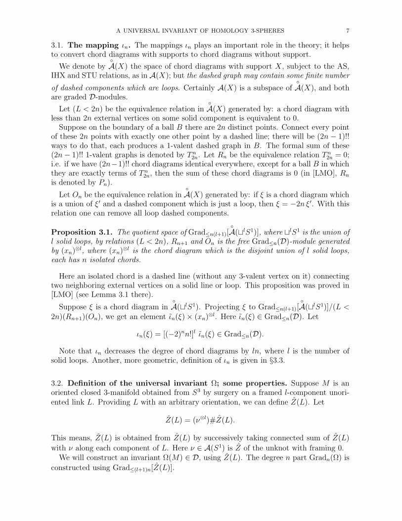
3.1. The mapping ιn. The mappings ιn plays an important role in the theory; it helpsto convert chord diagrams with supports to chord diagrams without support.

We denote by

A(X) the space of chord diagrams with support X, subject to the AS,IHX and STU relations, as in A(X); but the dashed graph may contain some finite number

of dashed components which are loops. Certainly A(X) is a subspace of

A(X), and bothare graded D-modules.

Let (L < 2n) be the equivalence relation in

A(X) generated by: a chord diagram withless than 2n external vertices on some solid component is equivalent to 0.

Suppose on the boundary of a ball B there are 2n distinct points. Connect every pointof these 2n points with exactly one other point by a dashed line; there will be (2n − 1)!!ways to do that, each produces a 1-valent dashed graph in B. The formal sum of these(2n − 1)!! 1-valent graphs is denoted by T n

2n. Let Rn be the equivalence relation T n2n = 0;

i.e. if we have (2n−1)!! chord diagrams identical everywhere, except for a ball B in whichthey are exactly terms of T n

2n, then the sum of these chord diagrams is 0 (in [LMO], Rn

is denoted by Pn).

Let On be the equivalence relation in

A(X) generated by: if ξ is a chord diagram whichis a union of ξ′ and a dashed component which is just a loop, then ξ = −2n ξ′. With thisrelation one can remove all loop dashed components.

Proposition 3.1. The quotient space of Grad≤n(l+1)[

A(⊔lS1)], where ⊔lS1 is the union ofl solid loops, by relations (L < 2n), Rn+1 and On is the free Grad≤n(D)-module generatedby (xn)⊗l, where (xn)⊗l is the chord diagram which is the disjoint union of l solid loops,each has n isolated chords.

Here an isolated chord is a dashed line (without any 3-valent vertex on it) connectingtwo neighboring external vertices on a solid line or loop. This proposition was proved in[LMO] (see Lemma 3.1 there).

Suppose ξ is a chord diagram in

A(⊔lS1). Projecting ξ to Grad≤n(l+1)[

A(⊔lS1)]/(L <2n)(Rn+1)(On), we get an element ιn(ξ) × (xn)⊗l. Here ιn(ξ) ∈ Grad≤n(D). Let

ιn(ξ) = [(−2)nn!]l ιn(ξ) ∈ Grad≤n(D).

Note that ιn decreases the degree of chord diagrams by ln, where l is the number ofsolid loops. Another, more geometric, definition of ιn is given in §3.3.

3.2. Definition of the universal invariant Ω; some properties. Suppose M is anoriented closed 3-manifold obtained from S3 by surgery on a framed l-component unori-ented link L. Providing L with an arbitrary orientation, we can define Z(L). Let

Z(L) = (ν⊗l)#Z(L).

This means, Z(L) is obtained from Z(L) by successively taking connected sum of Z(L)

with ν along each component of L. Here ν ∈ A(S1) is Z of the unknot with framing 0.We will construct an invariant Ω(M) ∈ D, using Z(L). The degree n part Gradn(Ω) is

constructed using Grad≤(l+1)n[Z(L)].

8 THANG T. Q. LE

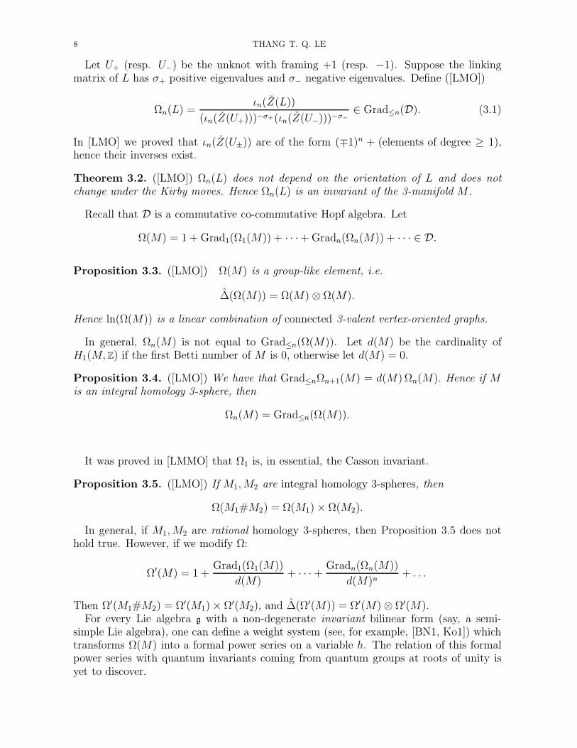
Let U+ (resp. U−) be the unknot with framing +1 (resp. −1). Suppose the linkingmatrix of L has σ+ positive eigenvalues and σ− negative eigenvalues. Define ([LMO])

Ωn(L) =ιn(Z(L))

(ιn(Z(U+)))−σ+(ιn(Z(U−)))−σ−

∈ Grad≤n(D). (3.1)

In [LMO] we proved that ιn(Z(U±)) are of the form (∓1)n + (elements of degree ≥ 1),hence their inverses exist.

Theorem 3.2. ([LMO]) Ωn(L) does not depend on the orientation of L and does notchange under the Kirby moves. Hence Ωn(L) is an invariant of the 3-manifold M .

Recall that D is a commutative co-commutative Hopf algebra. Let

Ω(M) = 1 + Grad1(Ω1(M)) + · · ·+ Gradn(Ωn(M)) + · · · ∈ D.

Proposition 3.3. ([LMO]) Ω(M) is a group-like element, i.e.

∆(Ω(M)) = Ω(M) ⊗ Ω(M).

Hence ln(Ω(M)) is a linear combination of connected 3-valent vertex-oriented graphs.

In general, Ωn(M) is not equal to Grad≤n(Ω(M)). Let d(M) be the cardinality ofH1(M, Z) if the first Betti number of M is 0, otherwise let d(M) = 0.

Proposition 3.4. ([LMO]) We have that Grad≤nΩn+1(M) = d(M) Ωn(M). Hence if Mis an integral homology 3-sphere, then

Ωn(M) = Grad≤n(Ω(M)).

It was proved in [LMMO] that Ω1 is, in essential, the Casson invariant.

Proposition 3.5. ([LMO]) If M1, M2 are integral homology 3-spheres, then

Ω(M1#M2) = Ω(M1) × Ω(M2).

In general, if M1, M2 are rational homology 3-spheres, then Proposition 3.5 does nothold true. However, if we modify Ω:

Ω′(M) = 1 +Grad1(Ω1(M))

d(M)+ · · ·+

Gradn(Ωn(M))

d(M)n+ . . .

Then Ω′(M1#M2) = Ω′(M1) × Ω′(M2), and ∆(Ω′(M)) = Ω′(M) ⊗ Ω′(M).For every Lie algebra g with a non-degenerate invariant bilinear form (say, a semi-

simple Lie algebra), one can define a weight system (see, for example, [BN1, Ko1]) whichtransforms Ω(M) into a formal power series on a variable h. The relation of this formalpower series with quantum invariants coming from quantum groups at roots of unity isyet to discover.

A UNIVERSAL INVARIANT OF HOMOLOGY 3-SPHERES 9

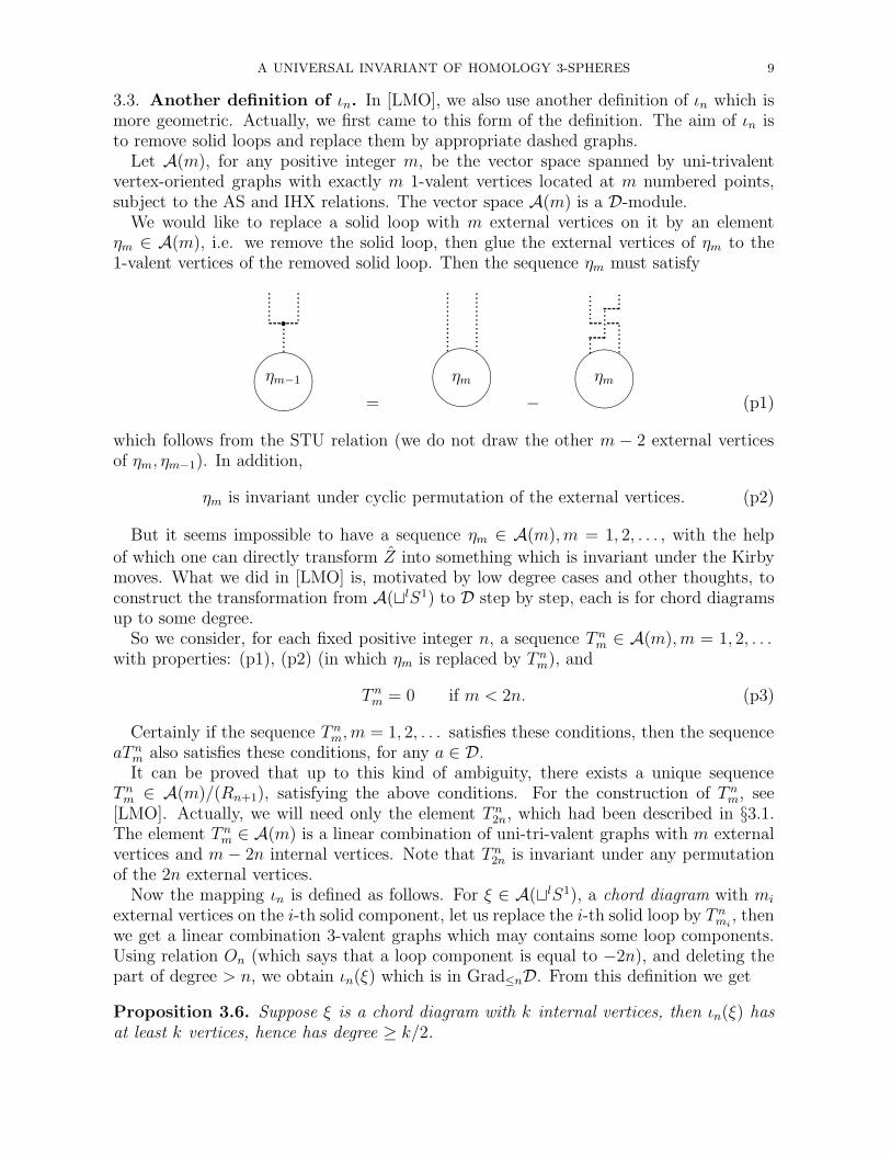
3.3. Another definition of ιn. In [LMO], we also use another definition of ιn which ismore geometric. Actually, we first came to this form of the definition. The aim of ιn isto remove solid loops and replace them by appropriate dashed graphs.

Let A(m), for any positive integer m, be the vector space spanned by uni-trivalentvertex-oriented graphs with exactly m 1-valent vertices located at m numbered points,subject to the AS and IHX relations. The vector space A(m) is a D-module.

We would like to replace a solid loop with m external vertices on it by an elementηm ∈ A(m), i.e. we remove the solid loop, then glue the external vertices of ηm to the1-valent vertices of the removed solid loop. Then the sequence ηm must satisfy

r

&%'$ηm−1

= &%'$

ηm

− &%'$

ηm

(p1)

which follows from the STU relation (we do not draw the other m − 2 external verticesof ηm, ηm−1). In addition,

ηm is invariant under cyclic permutation of the external vertices. (p2)

But it seems impossible to have a sequence ηm ∈ A(m), m = 1, 2, . . . , with the help

of which one can directly transform Z into something which is invariant under the Kirbymoves. What we did in [LMO] is, motivated by low degree cases and other thoughts, toconstruct the transformation from A(⊔lS1) to D step by step, each is for chord diagramsup to some degree.

So we consider, for each fixed positive integer n, a sequence T nm ∈ A(m), m = 1, 2, . . .

with properties: (p1), (p2) (in which ηm is replaced by T nm), and

T nm = 0 if m < 2n. (p3)

Certainly if the sequence T nm, m = 1, 2, . . . satisfies these conditions, then the sequence

aT nm also satisfies these conditions, for any a ∈ D.It can be proved that up to this kind of ambiguity, there exists a unique sequence

T nm ∈ A(m)/(Rn+1), satisfying the above conditions. For the construction of T n

m, see[LMO]. Actually, we will need only the element T n

2n, which had been described in §3.1.The element T n

m ∈ A(m) is a linear combination of uni-tri-valent graphs with m externalvertices and m − 2n internal vertices. Note that T n

2n is invariant under any permutationof the 2n external vertices.

Now the mapping ιn is defined as follows. For ξ ∈ A(⊔lS1), a chord diagram with mi

external vertices on the i-th solid component, let us replace the i-th solid loop by T nmi

, thenwe get a linear combination 3-valent graphs which may contains some loop components.Using relation On (which says that a loop component is equal to −2n), and deleting thepart of degree > n, we obtain ιn(ξ) which is in Grad≤nD. From this definition we get

Proposition 3.6. Suppose ξ is a chord diagram with k internal vertices, then ιn(ξ) hasat least k vertices, hence has degree ≥ k/2.

10 THANG T. Q. LE

3.4. Finite type invariants for homology 3-spheres. We briefly recall here somefundamental concepts, referring the reader to [Oh1, GO1, GL1].

Let M be the vector space over Q spanned by the set of all integral homology oriented3-spheres. Every invariant I of homology 3-spheres with values in a vector space can beuniquely extended to a linear mapping on M.

For a framed link L in M , let ML denote the 3-manifold obtained by performing Dehnsurgery on L. If K is a formal linear combination

∑i ciLi, where Li are framed links and

ci are numbers, then MK , by definition, is∑

i ciMLi∈ M.

When M is an oriented homology 3-sphere, there is a natural way to identify the set offramings of a knot in M with the set Z of integers; and we will use this identification.

A framed link L in M is unit-framed if the framing of each component is ±1; L isalgebraically split if the linking number of every two components is 0.

Let |L| be the number of components of L. Define

δ(L) =∑

L′⊂L

(−1)|L′|L′, (3.2)

where the sum is over all sublinks L′ ⊂ L, including the empty link.Consider the following decreasing filtration in M. Let Fn(M) be the vector space

generated by Mδ(L), where M is an arbitrary homology 3-sphere and L is a unit-framedand algebraically split n-component link in M .

Definition . ([Oh1])An invariant I of integral homology 3-spheres with values in a vectorspace is of order ≤ n if I(Fn+1(M)) = 0.

Ohtsuki showed that M/Fn(M) has finite dimension, see [Oh1]; this means the spaceof invariants of order less than n is finite-dimensional.

An important result (see [GL1, GO1]) is that F3n(M) = F3n+1(M) = F3n+2(M).Hence the set of invariants of order 3n is the same as the set of invariants of order 3n+2.

Every invariant I of order 3n with values in Q defines a linear form on M/F3n+1(M),hence restricts to a linear form on F3n(M)/F3n+1(M). As in knot theory, it’s importantto understand the structure of F3n(M)/F3n+1(M).

In [GO1], a surjective linear mapping O∗3n : Gradn(D) → F3n/F3n+1(M) was con-

structed. For a definition of O∗3n, see §5.1 below. It follows that if I is an invariant of

order 3n, then by combining with O∗3n, I defines a linear mapping from Gradn(D) to Q,

called the corresponding linear form of I. Note that if the corresponding linear form is 0,then the invariant is of order < 3n.

Is every linear mapping from Gradn(D) to Q the linear form of some invariant of order≤ 3n? (Question 1 in [GO1]). We will see that the answer is positive. This is equivalentto the fact that the above mapping O∗

3n is an isomorphism of vector spaces.

4. Main results

4.1. Universality of Ω. We will show the following

Theorem 4.1. (Main Theorem)a) For homology 3-spheres, Ωn is an invariant of order ≤ 3n.b) The mapping O∗

3n is an isomorphism, i.e. every linear form from Gradn(D) to Q isa linear form of some finite invariant of order 3n.

c) Ωn is a universal invariant of order 3n, i.e. if Ωn(M) = Ωn(M ′) then I(M) = I(M ′)for every invariant I of order ≤ 3n.

A UNIVERSAL INVARIANT OF HOMOLOGY 3-SPHERES 11

We need the following two lemmas, whose proofs will be presented in Section 5.

Lemma 4.2. Suppose that Γ is a 3-valent vertex-oriented graph in D of degree n. Thenfor any representative α(Γ) of O∗

3n(Γ) in F3n(M), one has

Ωn(α(Γ)) = (−1)nΓ + Ωn(M1), (4.1)

where M1 is in F3n+3(M).

Lemma 4.3. If N ∈ F6n+1(M), then Ωn(N) = 0.

This lemma is certainly weaker than part a) of Main Theorem.

Proof. [of Main Theorem]a) Suppose N ∈ F3n+1(M) = F3n+3(M) we have to show that Ωn(N) = 0.Since O∗

3n+3 : Gradn+1(D) → F3n+3(M)/F3n+6(M) is surjective, there is Γ1 ∈ Gradn+1(D)such that

N − α(Γ1) = N1 ∈ F3n+6(M),

where α(Γ1) is any representative of O∗3n+3(Γ1) in F3n+3(M). Apply Ωn+1 to both sides,

using Lemma 4.2 with n replaced by n + 1; we see that, for some M1 ∈ F3n+6(M),

Ωn+1(N) = ±Γ1 + Ωn+1(N1) + Ωn+1(M1) = ±Γ1 + Ω(N1 + M1).

Since Ωn = Grad≤nΩn+1 (see Proposition 3.4) and Γ1 is of degree n + 1, one has

Ωn(N) = Ωn(M1 + N1).

Here (M1 + N1) is in F3n+6, while N is in F3n+3(M). Repeat this argument n times, onefinds N ′ in F6m+3(M) such that

Ωn(N) = ΩnN ′.

Now Lemma 4.3 says that Ωn(N ′) = 0. This completes the proof of a).b) We will show an inverse of O∗

3n : Gradn(D) → F3n(M)/F3n+3(M). Let us considerequation (4.1) again. Since M1 in the equation is in F3n+3(M), by part a), we haveΩn(M1) = 0. Hence

Ωn(α(Γ)) = (−1)nΓ.

This is true for every representative α(Γ) of O∗3n(Γ) in F3n(M), hence (−1)nΩn restricts to

a well-defined linear mapping from F3n(M)/F3n+3(M) to GradnD, which, by the aboveidentity, is inverse to O∗

3n.c) We use induction on n. Suppose Ωn(M) = Ωn(M ′) ∈ Grad≤n(D) and I is an invariant

of order n with values in Q. Let W : Gradn(D) → Q be the corresponding linear form ofI. Let I1 = W (Gradn(Ωn)). Then I1 is an invariant of order ≤ 3n and I1(M) = I1(M

′).Note that I − I1 is an invariant of order ≤ 3n. It is not hard to verify that the

corresponding linear form of I − I1 from Gradn(D) to Q is 0, hence I − I1 is of order≤ (3n − 1). By induction, (I − I1)(M) = (I − I1)(M

′). Hence I(M) = I(M ′).

Let the product of two homology 3-spheres be their connected sum. The unit is S3.Define a co-product: ∆(M) = M ⊗ M , and co-unit: ε(M) = 1, for every homology3-sphere M . Then M becomes a commutative co-commutative Hopf algebra.

It is easy to see that the product is compatible with the filtration

M = F0M ⊃ F3M ⊃ · · · ⊃ F3n(M) . . .

This means, if N1 ∈ Fn1(M) and N2 ∈ Fn2

(M), then their product is in Fn1+n2(M).

12 THANG T. Q. LE

Hence the algebra structure of M induces an algebra structure on the associated (com-plete) graded vector space

GM =∞∏

i=0

F3i(M)/F3i+3(M).

A nice interpretation of the main theorem is the following.

Theorem 4.4. a) The mapping Ω : M → D is a Hopf algebra homomorphism whichmaps F3n(M) to Grad≥nD.

b) Ω induces an algebra isomorphism between GM and D.

This theorem follows immediately from the previous one and Propositions 3.3, 3.5. Partb) shows that GM has a structure of a commutative co-commutative Hopf algebra.

4.2. Some further properties of Ω.

Proposition 4.5. a) Ωn is of order exactly 3n.b) For every n there is an integral homology 3-sphere Mn such that Ω(Mn) = 1 +

degree ≥ n, and the n-th degree part is not 0.

Proof. a) This is equivalent to the fact that Gradn(D) has positive dimension. It’s enoughto show that there is a non-zero linear form on Gradn(D). One can use the weight systemcoming from simple Lie algebra, as defined in [Ko1, BN1, LM2], to define non-zero linearform. The details are left for the reader. a) also follows from b).

b) Consider a solid loop and a dashed loop, each has 2n marked points x1, x2, . . . , x2n

and y1, y2, . . . , y2n, counting counterclockwise. Connect xi with yi by a dashed line, forevery i = 1, 2, . . . , 2n, we get a chord diagram ξn on a solid loop. In [Ng], a knot Kwas constructed with property that for every knot invariant I of degree < 2n, we haveI(K) = I(unknot) and for every invariant I of degree 2n we have I(K) = I(ξn). It followsthat if K has framing 0, then

Z(K) = ν(1 + ξn) + (elements of degree > 2n).

Hence if K ′ is the knot K with framing 1, we have

Z(K ′) = ν2eθ/2(1 + ξn) + (elements of degree > 2n).

Here θ ∈ A(S1) is the chord diagram of degree 1 with one isolated chord; eθ/2 is thecontribution of framing 1 (see [LM2], Theorem 3). Let Mn be obtained by Dehn surgeryon K ′, then, by definition

Ωn(Mn) =ιn(Z(K ′))

ιn(U+)=

ιn[ν2eθ/2(1 + ξn)]

ιn(ν2eθ/2).

Since ξn is of degree 2n, ιn annihilates any chord diagram in A(S1) of degree > 2n, andιn(U+) = ιn(ν2eθ/2) = (−1)n + ..., we see that Ωn(Mn) = 1 + (−1)nιn(ξn).

Using the definition of ιn (the one with T n2n described in §3.3), combining with sl2-weight

system, one can prove that ιn(ξn) 6= 0.

In [Lin], X. S. Lin asked whether there exists an operation, similar to the Stanford onein the knot case, on homology 3-spheres which does not alter the values of any invariantof order ≤ n. We now present such an operation.

Suppose M is obtained by Dehn surgery on a unit-framed algebraically split link L.Suppose that T is a part of L which is a trivial tangle with m strands. Let Gj(Pm), j =

A UNIVERSAL INVARIANT OF HOMOLOGY 3-SPHERES 13

0, 1, 2, . . . be the lower central series of the pure braid group Pm on m strands, defined byG0(Pm) = Pm, Gj+1(Pm) = [Gj(Pm), Pm]. Replacing T by an element γ in the (2n + 2)-th group G2n+2(Pm), we obtain a unit-framed algebraically split link L′. The homology3-sphere S3

L′ is said to be obtained from M by an sn operation.

Proposition 4.6. If M ′ is obtained from M by an sn operation, then Ωn(M) = Ωn(M ′).Hence the values of any invariant of order ≤ 3n on M and on M ′ are the same.

Proof. We first consider Z(γ) ∈ Pm. By a result of Stanford [Sta] (see also [Koh]), thevalues of any pure braid invariant of order ≤ (2n + 1) on T (the trivial tangle) and γ arethe same. Hence

Grad≤(2n+1)Z(γ) = 1.

From Theorem 4.2 of [LM3], it follows that Z(γ) is a group-like element, i.e. Z(γ) =exp(ξ), where ξ is primitive. The above identity shows that ξ is a linear combination ofchord diagrams of degree ≥ (2n + 2). Hence from Proposition 2.1 one sees that

Z(γ) = 1 + (elements of i-filter ≥ (2n + 1)).

Since ιn annihilates any element of i-filter ≥ (2n+1), we have that Ωn(M) = Ωn(M ′).

Note that we proved this fact only for invariants with rational values. It would beinteresting to give a direct geometric proof of this fact, and to establish the same fact forinvariants with values in any abelian group.

From this proposition, it is easy to construct, for any given homology 3-sphere M andany positive integer n, infinitely many homology 3-spheres which are indistinguishablefrom M by all invariants of order ≤ n.

4.3. Some other corollaries; remarks. X. S. Lin proved (see [Lin])

Proposition 4.7. The space of finite type invariants of homology 3-spheres with rationalvalues is a commutative co-commutative Hopf algebra.

Here this fact is a consequence of Theorem 4.4, b), as observed in [GO1], Remark 1.10.Suppose I is an invariant of integral homology 3-spheres, K is a knot in S3. Let us

define λI(K) = I(S3K), where we provide K with framing 1.

Proposition 4.8. If I is a homology 3-sphere invariant of order 3n, then λI is a knotinvariant of order 2n.

This had been conjectured by Garoufalidis, and proved by Habegger, see [Hab]. Herethis fact follows easily from the main theorem: for a knot K, the universal invariantΩn(S3

K) is computed using Grad≤2n(Z(K)), hence IΩn(K) is derived from Grad≤2nZ(K)

which is a knot invariant of order ≤ 2n.

Remark . 1. The main theorem can be reformulated and proved (in a similar way) forrational homology 3-spheres, see [GO2] for theory of finite type invariants of rationalhomology 3-spheres. The details will appear elsewhere.

2. The construction of Ω suggests that the relation between Ω, combined with sl2weight, and sl2 quantum invariant at roots of unity maybe expressed through Ohtsukipolynomial in [Oh2], or the invariant defined in [Oh3].

14 THANG T. Q. LE

4.4. Groups of homology 3-spheres. In analogy with the knot case (see [Gus, Ng,NgS]), we say that two integral homology spheres M1, M2 are Vn-equivalent if they areindistinguishable by any rational invariant of order ≤ n; or the same as: (M1 − M2) ∈F3n+1(M), or Ωn(M1) = Ωn(M2).

Let VMn be the set of all homology 3-spheres, regarded up to the Vn-equivalencerelation. This set VMn is a semigroup, where the product is the connected sum.

Theorem 4.9. For every connected 3-valent vertex-oriented graph Γ of degree n, thereare homology 3-spheres M±(Γ) such that

Ω(M±(Γ)) = 1 + ±Γ + (elements of degree > n).

Moreover, M±(Γ) are obtained by Dehn surgery on links of n components.

This is stronger than proposition 4.5. From Theorem 4.9, one gets

Theorem 4.10. The semi-group VMn is a group. This means, for every homology 3-sphere M , there is another homology 3-spheres M ′ such that M#M ′ is Vn-equivalent to 0.

The group VMn is free abelian of rank equal to the dimension of the subspace ofGradn(D), spanned by connected 3-valent vertex-oriented graphs.

This answers the first part of question 2 in [Lin].Proofs of Theorems 4.9 and 4.10 will appear elsewhere.

5. Proofs

5.1. The mapping O∗3n. Let’s consider a 3-valent vertex-oriented graph Γ of degree n

in R3. Like with links, we can represent Γ using a generic projection on the plane withdecoration at every double point to indicate over/under-crossing. We suppose that Γ isequal to this projection everywhere except for a neighborhood of the double points, thatthe orientation at every vertex is given by counterclockwise direction of the plane, andthat the three edges incident to a 3-valent vertex is going downwards in a neighborhoodof the vertex as in Figure 4. Here edges of Γ are depicted by solid lines.

Γ has 2n trivalent vertices and 3n edges. Using 2n pairs of horizontal lines on the plane,each pair consists of a line above and a line below a vertex, we can decompose Γ as:

Γ = T1V1T2V2 . . . T2nV2nT2n+1. (5.1)

Here Ti are some non-oriented tangles while Vi are trivial tangles with a 3-valent vertexpart as in Figure 4; and product in the right hand side means “placing on top”.

@@

@

Figure 4. Vi

Now we define β(Ti) and β(Vi) as follows. Let β(Ti) be the tangle obtained by replacingeach component of Ti by a pair of parallel push-offs (on the plane) of this component.The orientation on β(Ti) is chosen so that at boundary points of a pair of push-offs, theleft boundary point is pointing upwards, and the right boundary point downwards.

A UNIVERSAL INVARIANT OF HOMOLOGY 3-SPHERES 15

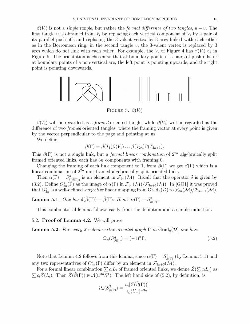
β(Vi) is not a single tangle, but rather the formal difference of two tangles, u− v. Thefirst tangle u is obtained from Vi by replacing each vertical component of Vi by a pair ofits parallel push-offs and replacing the 3-valent vertex by 3 arcs linked with each otheras in the Borromean ring; in the second tangle v, the 3-valent vertex is replaced by 3arcs which do not link with each other. For example, the Vi of Figure 4 has β(Vi) as inFigure 5. The orientation is chosen so that at boundary points of a pairs of push-offs, orat boundary points of a non-vertical arc, the left point is pointing upwards, and the rightpoint is pointing downwards.

@@

ll

ll

$−

Figure 5. β(Vi)

β(Ti) will be regarded as a framed oriented tangle, while β(Vi) will be regarded as thedifference of two framed oriented tangles, where the framing vector at every point is givenby the vector perpendicular to the page and pointing at us.

We define

β(Γ) = β(T1)β(V1) . . . β(V2n)β(T2n+1).

This β(Γ) is not a single link, but a formal linear combination of 22n algebraically splitframed oriented links, each has 3n components with framing 0.

Changing the framing of each link component to 1, from β(Γ) we get β(Γ) which is alinear combination of 22n unit-framed algebraically split oriented links.

Then α(Γ) = S3δ(β(Γ))

is an element in F3n(M). Recall that the operator δ is given by

(3.2). Define O∗3n(Γ) as the image of α(Γ) in F3n(M)/F3n+1(M). In [GO1] it was proved

that O∗3n is a well-defined surjective linear mapping from Gradn(D) to F3n(M)/F3n+1(M).

Lemma 5.1. One has δ(β(Γ)) = β(Γ). Hence α(Γ) = S3β(Γ)

.

This combinatorial lemma follows easily from the definition and a simple induction.

5.2. Proof of Lemma 4.2. We will prove

Lemma 5.2. For every 3-valent vertex-oriented graph Γ in Gradn(D) one has:

Ωn(S3β(Γ)

) = (−1)nΓ. (5.2)

Note that Lemma 4.2 follows from this lemma, since α(Γ) = S3β(Γ)

(by Lemma 5.1) and

any two representatives of O∗3n(Γ) differ by an element in F3n+3(M).

For a formal linear combination∑

ciLi of framed oriented links, we define Z(∑

ciLi) as∑

ciZ(Li). Then Z(β(Γ)) ∈ A(⊔3nS1). The left hand side of (5.2), by definition, is

Ωn(S3β(Γ)

) =ιn[Z(β(Γ))]

ιn(U+)−3n.

16 THANG T. Q. LE

Since ιn(U+) has the form (−1)n+ elements of degree ≥ 1 (see [LMO]), in order to prove(5.2) it suffices to show that

ιn[Z(β(Γ))] = Γ. (5.3)

For Vi in the decomposition (5.1) of Γ, β(Vi) = u−v, where u−v are tangles in Figure 5.

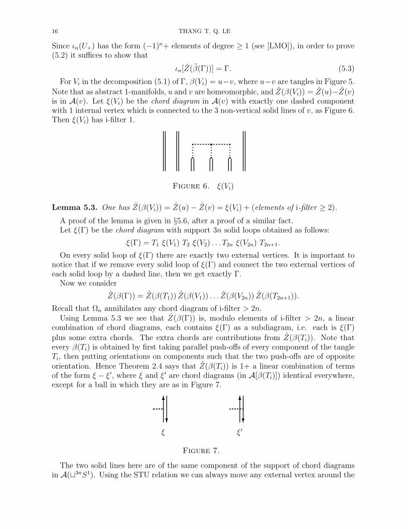
Note that as abstract 1-manifolds, u and v are homeomorphic, and Z(β(Vi)) = Z(u)−Z(v)is in A(v). Let ξ(Vi) be the chord diagram in A(v) with exactly one dashed componentwith 1 internal vertex which is connected to the 3 non-vertical solid lines of v, as Figure 6.Then ξ(Vi) has i-filter 1.

r

Figure 6. ξ(Vi)

Lemma 5.3. One has Z(β(Vi)) = Z(u) − Z(v) = ξ(Vi) + (elements of i-filter ≥ 2).

A proof of the lemma is given in §5.6, after a proof of a similar fact.Let ξ(Γ) be the chord diagram with support 3n solid loops obtained as follows:

ξ(Γ) = T1 ξ(V1) T2 ξ(V2) . . . T2n ξ(V2n) T2n+1.

On every solid loop of ξ(Γ) there are exactly two external vertices. It is important tonotice that if we remove every solid loop of ξ(Γ) and connect the two external vertices ofeach solid loop by a dashed line, then we get exactly Γ.

Now we consider

Z(β(Γ)) = Z(β(T1)) Z(β(V1)) . . . Z(β(V2n)) Z(β(T2n+1)).

Recall that Ωn annihilates any chord diagram of i-filter > 2n.Using Lemma 5.3 we see that Z(β(Γ)) is, modulo elements of i-filter > 2n, a linear

combination of chord diagrams, each contains ξ(Γ) as a subdiagram, i.e. each is ξ(Γ)

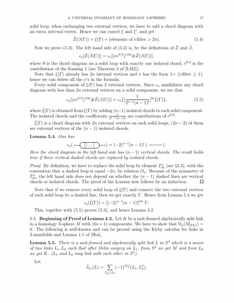
plus some extra chords. The extra chords are contributions from Z(β(Ti)). Note thatevery β(Ti) is obtained by first taking parallel push-offs of every component of the tangleTi, then putting orientations on components such that the two push-offs are of oppositeorientation. Hence Theorem 2.4 says that Z(β(Ti)) is 1+ a linear combination of termsof the form ξ − ξ′, where ξ and ξ′ are chord diagrams (in A[β(Ti)]) identical everywhere,except for a ball in which they are as in Figure 7.

ξ ξ′

6

? ?

6

Figure 7.

The two solid lines here are of the same component of the support of chord diagramsin A(⊔3nS1). Using the STU relation we can always move any external vertex around the

A UNIVERSAL INVARIANT OF HOMOLOGY 3-SPHERES 17

solid loop; when exchanging two external vertices, we have to add a chord diagram withan extra internal vertex. Hence we can cancel ξ and ξ′, and get

Z(β(Γ)) = ξ(Γ) + (elements of i-filter > 2n). (5.4)

Now we prove (5.3). The left hand side of (5.3) is, by the definitions of Z and β,

ιn[Z(β(Γ))] = ιn[(νeθ/2)⊗3n#Z(β(Γ))],

where θ is the chord diagram on a solid loop with exactly one isolated chord; eθ/2 is thecontribution of the framing 1 (see Theorem 3 of [LM2]).

Note that ξ(Γ) already has 2n internal vertices and ν has the form 1+ (i-filter ≥ 1),hence we can delete all the ν’s in the formula.

Every solid component of ξ(Γ) has 2 external vertices. Since ιn annihilates any chorddiagram with less than 2n external vertices on a solid component, we see that

ιn[(νeθ/2)⊗3n#Z(β(Γ))] = ιn[1

2n−1(n − 1)!]3nξ(Γ), (5.5)

where ξ(Γ) is obtained from ξ(Γ) by adding (n−1) isolated chords to each solid component.The isolated chords and the coefficients 1

2n−1(n−1)!are contributions of eθ/2.

ξ(Γ) is a chord diagram with 2n external vertices on each solid loops, (2n− 2) of themare external vertices of the (n − 1) isolated chords.

Lemma 5.4. One has

ιn( · · · ) = (−2)n−1(n − 1)! ( ).

Here the chord diagram in the left hand side has (n− 1) vertical chords. The result holdstrue if these vertical dashed chords are replaced by isolated chords.

Proof. By definition, we have to replace the solid loop by element T n2n (see §3.3), with the

convention that a dashed loop is equal −2n, by relation On. Because of the symmetry ofT n

2n, the left hand side does not depend on whether the (n − 1) dashed lines are verticalchords or isolated chords. The proof of the Lemma now follows by an induction.

Note that if we remove every solid loop of ξ(Γ) and connect the two external verticesof each solid loop be a dashed line, then we get exactly Γ. Hence from Lemma 5.4 we get

ιn(ξ(Γ)) = [(−2)n−1(n − 1)!]3n Γ.

This, together with (5.5) proves (5.3), and hence Lemma 4.2.

5.3. Beginning of Proof of Lemma 4.3. Let K be a unit-framed algebraically split linkin a homology 3-sphere M with (6n+1) components. We have to show that Ωn(Mδ(K)) =0. The following is well-known and can be proved using the Kirby calculus for links in3-manifolds and Lemma 1.1 of [Hos].

Lemma 5.5. There is a unit-framed and algebraically split link L in S3 which is a unionof two links L1, L2 such that after Dehn surgery on L1, from S3 we get M and from L2

we get K. (L1 and L2 may link with each other in S3).

LetδL2

(L) =∑

L′

2⊂L2

(−1)|L′

2|(L1, L

′′2),

18 THANG T. Q. LE

where the sum is over the set of all sublinks L′2 of L2; and (L1, L

′′2) is the link obtained

from L = (L1, L2) by replacing every component of L2 \ L′2 by a trivial knot with the

same framing; the trivial knots are not linked with each other nor with L.Let (L1, L

′2) be obtained from (L1, L2) by replacing L2 with L′

2.By definition,

Ωn(Mδ(L)) =∑

L′

2⊂L2

(−1)|L′

2|Ωn[S3

(L1,L′

2)] =

∑

L′

2⊂L2

(−1)|L′

2| ιn(Z(L1, L

′2))

ιn(U+)−σ+(L1,L′

2)ιn(U−)−σ−(L1,L′

2).

Note that U± are the trivial knots with framing ±1, and that ιn(a⊔ b) = ιn(a)ιn(b) fortwo links a, b. Using the same denominator ιn(U+)−σ+ιn(U−)−σ−, where σ± = σ±(L1, L2),for all the terms of the last sum, we arrive at the following important formula:

Ωn(Mδ(K)) =ιn[Z(δL2

(L1, L2))]

ιn(U+)−σ+ιn(U−)−σ−

.

Hence in order to prove Lemma 4.3, it’s sufficient to prove that

ιn[Z(δL2(L1, L2))] = 0 (5.6)

Here (L1, L2) is a unit-framed algebraically split link in S3 with |L2| = 6n + 1.The proof of (5.6) may look complicated, but the idea is simple. The point is that

δL2(L) is a repeated difference formula. The simplest case is when |L2| = 1 (only one

step). In this case δL2(L) = L − L′, where L′ is obtained from L by replacing the only

component of L2 by a trivial knot with the same framing. Then it can be proved thatZ(L − L′) is of i-filter ≥ 1. (The reason for this phenomenon is that the linking numberof L2 and other components is 0).

When |L2| > 1 we have a repeated difference sum for Z(δL2(L1, L2)); we expect that

Z(δL2(L1, L2)) has i-filter ≥ (2n+1), if |L2| is sufficiently large (|L2| = 6n+1 is enough).

It follows then ιn[Z(δL2(L1, L2))] = 0. A rigorous proof requires a lot of technical stuff.

5.4. Some preparations. Let Y be a submanifold of X; Y consists of several compo-nents of X. We say that an element ξ ∈ A(X) is i-near Y if ξ is a linear combination ofchord diagrams, each has internal vertices near every component of Y . Here an internalvertex is near a solid component if the vertex is connected to the solid component by adashed line of the dashed graph.

Recall that Pm, the space of chord diagrams on m numbered solid lines, is a co-commutative Hopf algebra. The space of primitive elements is spanned by chord diagramswith connected dashed graph.

A tangle consisting of m strings (no loops) such that the two end points of each stringproject vertically to the same point is called a string link. Suppose that T is an m-component framed string link whose orientation at every boundary points is downward. Acorollary of Theorem 4.2 of [LM3] is that Z(T ) ∈ Pm is group-like. Hence Z(T ) = exp(ξ),where ξ is primitive.

Suppose T ′ is obtained from T by removing a component C. Let εC : Pm → Pm−1

be the linear mapping which send a chord diagram ξ ∈ Pm to εC(ξ) obtained from ξ byremoving the solid line C if there is no external vertex on C; otherwise εC(ξ) = 0.

The relation between Z(T ) and Z(T ′) is expressed by (see [LM1, LM2]):

Z(T ′) = εC [Z(T )]. (5.7)

A UNIVERSAL INVARIANT OF HOMOLOGY 3-SPHERES 19

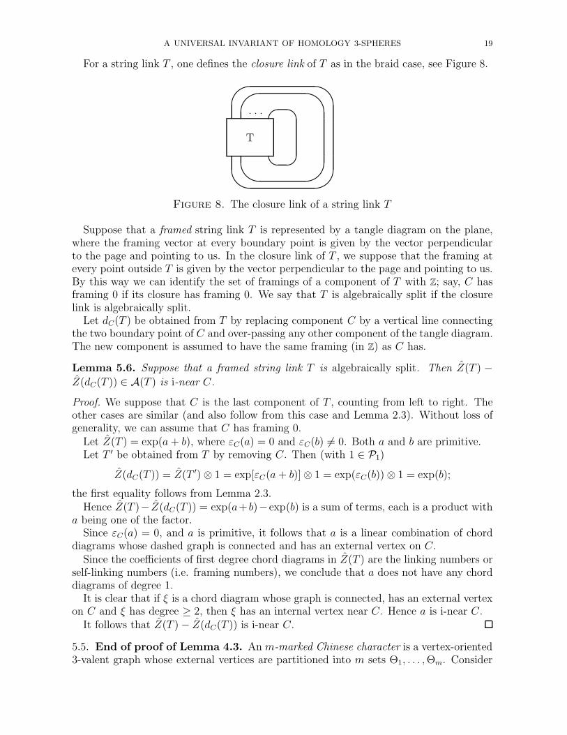
For a string link T , one defines the closure link of T as in the braid case, see Figure 8.

T

& %& %

' $' $ . . .

Figure 8. The closure link of a string link T

Suppose that a framed string link T is represented by a tangle diagram on the plane,where the framing vector at every boundary point is given by the vector perpendicularto the page and pointing to us. In the closure link of T , we suppose that the framing atevery point outside T is given by the vector perpendicular to the page and pointing to us.By this way we can identify the set of framings of a component of T with Z; say, C hasframing 0 if its closure has framing 0. We say that T is algebraically split if the closurelink is algebraically split.

Let dC(T ) be obtained from T by replacing component C by a vertical line connectingthe two boundary point of C and over-passing any other component of the tangle diagram.The new component is assumed to have the same framing (in Z) as C has.

Lemma 5.6. Suppose that a framed string link T is algebraically split. Then Z(T ) −Z(dC(T )) ∈ A(T ) is i-near C.

Proof. We suppose that C is the last component of T , counting from left to right. Theother cases are similar (and also follow from this case and Lemma 2.3). Without loss ofgenerality, we can assume that C has framing 0.

Let Z(T ) = exp(a + b), where εC(a) = 0 and εC(b) 6= 0. Both a and b are primitive.Let T ′ be obtained from T by removing C. Then (with 1 ∈ P1)

Z(dC(T )) = Z(T ′) ⊗ 1 = exp[εC(a + b)] ⊗ 1 = exp(εC(b)) ⊗ 1 = exp(b);

the first equality follows from Lemma 2.3.Hence Z(T )− Z(dC(T )) = exp(a+ b)−exp(b) is a sum of terms, each is a product with

a being one of the factor.Since εC(a) = 0, and a is primitive, it follows that a is a linear combination of chord

diagrams whose dashed graph is connected and has an external vertex on C.Since the coefficients of first degree chord diagrams in Z(T ) are the linking numbers or

self-linking numbers (i.e. framing numbers), we conclude that a does not have any chorddiagrams of degree 1.

It is clear that if ξ is a chord diagram whose graph is connected, has an external vertexon C and ξ has degree ≥ 2, then ξ has an internal vertex near C. Hence a is i-near C.

It follows that Z(T ) − Z(dC(T )) is i-near C.

5.5. End of proof of Lemma 4.3. An m-marked Chinese character is a vertex-oriented3-valent graph whose external vertices are partitioned into m sets Θ1, . . . , Θm. Consider

20 THANG T. Q. LE

the space Em spanned by m-marked Chinese characters, subject to the AS and IHXrelations.

Let s be a subset of 1, 2, . . . , m. An element ξ ∈ Em is i-near s if ξ is a linearcombination of m-marked Chinese characters, each has internal vertices near Θj for everyj ∈ s. Here an internal vertex is near Θj if it is connected to an external vertex in Θj bya dashed line.

Consider the linear mapping χ : Em → Pm, defined as follows. Suppose an m-markedChinese character ξ has ki external vertices in Θi, i = 1, 2, . . . , m. There are ki! ways toput the vertices from Θi on the i-th solid string; and each of the k1! k2! . . . km! possibilitiesgive us a chord diagram in Pm. Summing up all such chord diagrams, we get χ(ξ).

It is known that χ is an isomorphism of vector spaces (see Theorem 9 in [LM2]). Thecase when m = 1 was first proved by Kontsevich; for a detailed proof of the case m = 1see [BN1] (Theorem 6). The inverse of χ is obtained by a symmetrizing process.

It follows from the definitions of χ and its inverse that

Proposition 5.7. For the j-th component C of the support of Pm, χ : Em → Pm mapsisomorphically the subspace of i-near j elements to the subspace of i-near C elements.

An important fact is that the AS and IHX relations preserve the property to have aninternal vertex near Θj . Hence the space spanned by m-marked Chinese characters noti-near j has 0 intersection with the space of elements i-near j, for every j ∈ 1, 2, . . . , m.The similar fact does not hold true for Pm, due to the STU relation. It follows that

Proposition 5.8. Suppose that ξ ∈ Em is i-near j for each j ∈ s, where s is a subset of1, 2, . . . , m, then ξ is i-near s.

From this proposition and Proposition 5.7 we have

Proposition 5.9. If ξ ∈ Pm is i-near C for each component C of Y , then ξ is i-near Y .

Now we prove Lemma 4.3. We need to prove (5.6). We will first prove that Z(δL2(L))

is i-near L2, i.e., Z(δL2(L)) is a linear combination of chord diagrams, each has internal

vertices near every component of L2. Since each internal vertex can be near at most 3different solid components, and since |L2| = 6n + 1, it then follows that Z(δL2

(L)) has

i-filter ≥ 2n + 1. Hence Ωn[Z(δL2(L))] = 0.

We can represent L = (L1, L2) as the closure of an m-component string link T . Wesuppose T is the union of Ti, i = 1, 2, where the components of Ti correspond to thecomponents of Li. For a sub-tangle T ′

2 ⊂ T2, let (T1, T′′2 ) be the tangle obtained from

T = (T1, T2) by successively applying dC to T , where C runs the set of all components ofT2 \ T ′

2 and dC is as in Lemma 5.6. Let

δT2(T ) =

∑

T ′

2⊂T2

(−1)|T′

2|(T1, T

′′2 ).

It is easy to see that for every component C of T2, the sum Z(δT2(T )) can be represented

as a finite sum of terms, each is of the form Z(V ) − Z(dC(V )). Hence by Lemma 5.6,

Z(δT2(T )) ∈ Pm is i-near C. Since this is true for every component C in T2, Proposition

5.9 says that Z(δT2(T )) is i-near T2.

Observe that δT2(T ) is a linear combination of framed string links; and the closure of

δT2(T ) is exactly δL2

(L). By Lemma 2.3 and property (2.1) we have

Z(δL2(L)) = a[Z(δT2

(T )) ⊗ 1]b,

A UNIVERSAL INVARIANT OF HOMOLOGY 3-SPHERES 21

where 1 ∈ Pm is the chord diagram without dashed graph, and a, b are some linearcombinations of chord diagrams. It follows that Z(δL2

(L)) is i-near L2. As argued above,

since |L2| ≥ 6n + 1, we get Ωn[Z(δL2(L))] = 0. This completes the proof of (5.6), and

hence that of Lemma 4.3.

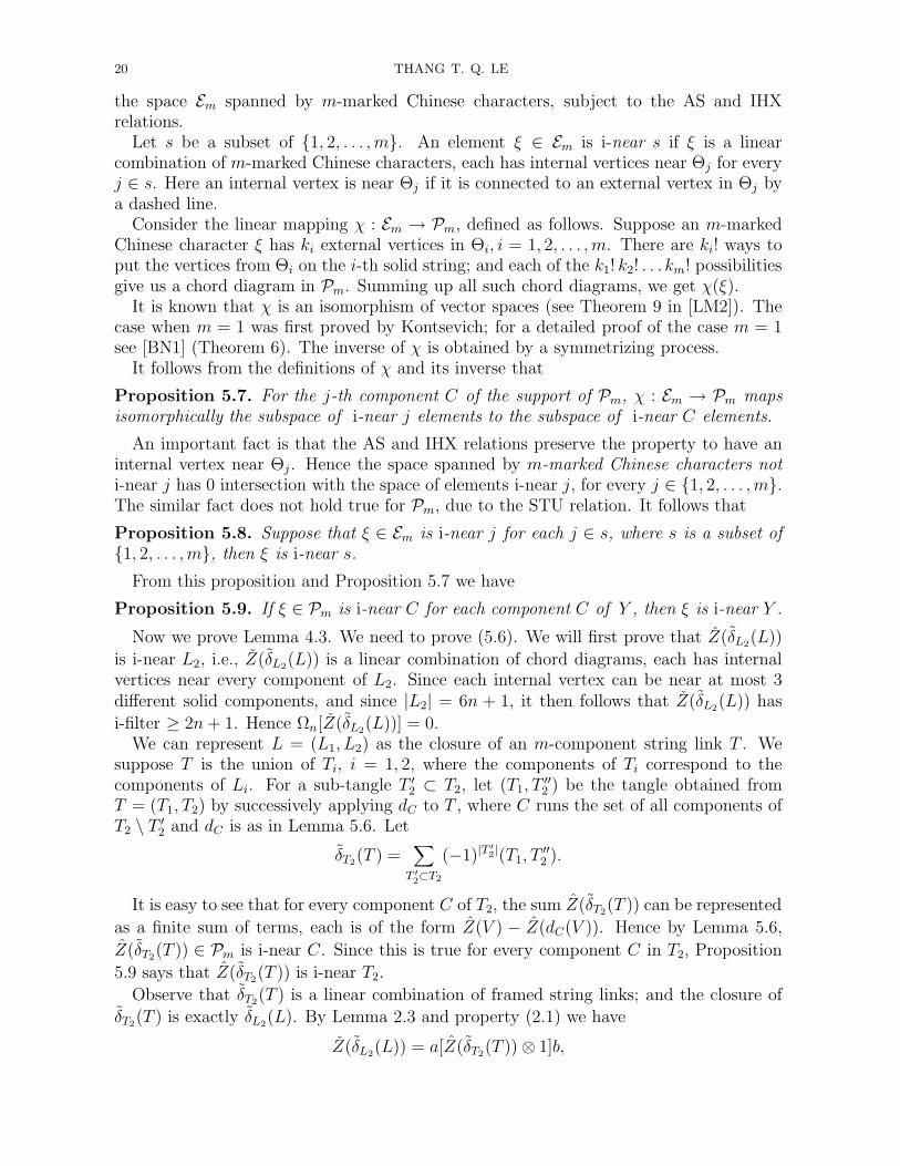
5.6. Proof of Lemma 5.3. By Lemma 2.3, it suffices to consider the case when Vi doesnot contain any vertical line. Then β(Vi) = u − v, where v is 3 arcs not linked with eachother, while u is 3 arcs linked with each other like in the Borromean link.

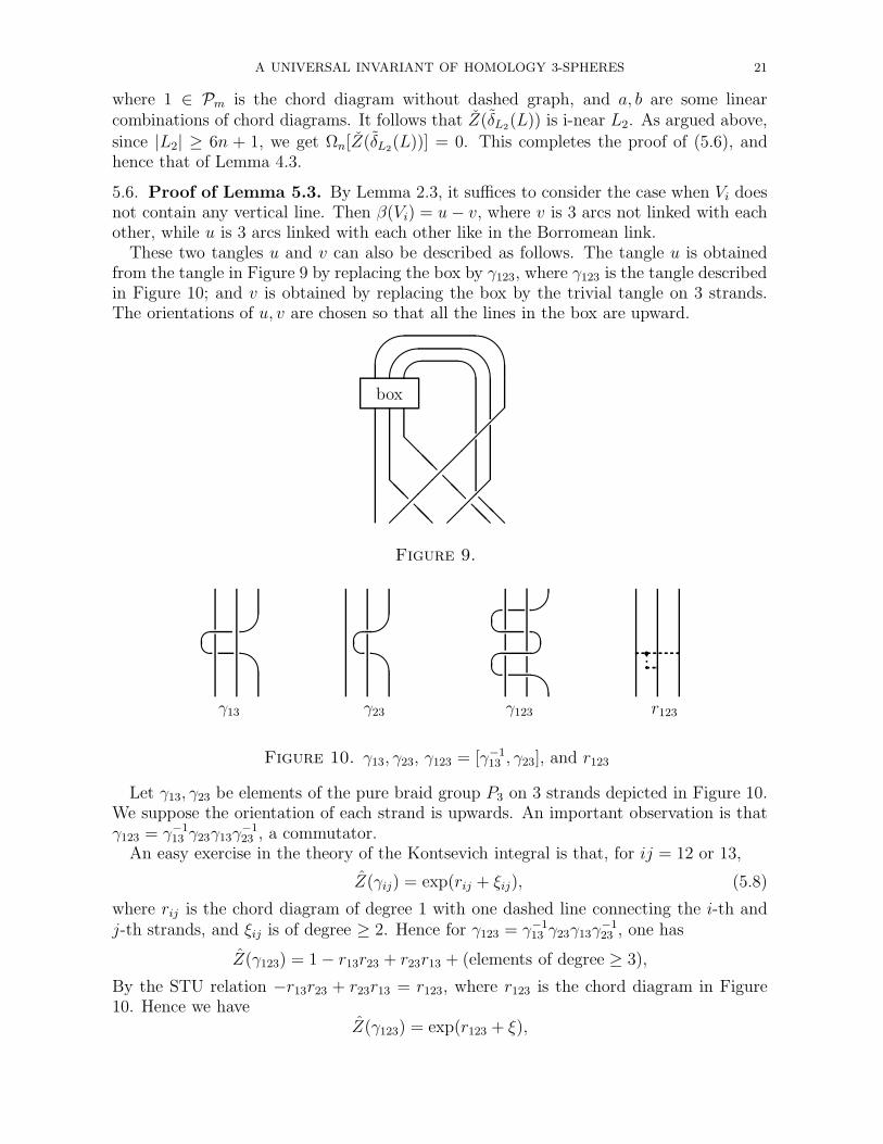
These two tangles u and v can also be described as follows. The tangle u is obtainedfrom the tangle in Figure 9 by replacing the box by γ123, where γ123 is the tangle describedin Figure 10; and v is obtained by replacing the box by the trivial tangle on 3 strands.The orientations of u, v are chosen so that all the lines in the box are upward.' $' $

box

@@ @@ @

@

@@

@@@

@@

Figure 9.

γ13

γ23

γ123

rr123

Figure 10. γ13, γ23, γ123 = [γ−113 , γ23], and r123

Let γ13, γ23 be elements of the pure braid group P3 on 3 strands depicted in Figure 10.We suppose the orientation of each strand is upwards. An important observation is thatγ123 = γ−1

13 γ23γ13γ−123 , a commutator.

An easy exercise in the theory of the Kontsevich integral is that, for ij = 12 or 13,

Z(γij) = exp(rij + ξij), (5.8)

where rij is the chord diagram of degree 1 with one dashed line connecting the i-th andj-th strands, and ξij is of degree ≥ 2. Hence for γ123 = γ−1

13 γ23γ13γ−123 , one has

Z(γ123) = 1 − r13r23 + r23r13 + (elements of degree ≥ 3),

By the STU relation −r13r23 + r23r13 = r123, where r123 is the chord diagram in Figure10. Hence we have

Z(γ123) = exp(r123 + ξ),

22 THANG T. Q. LE

where ξ is primitive and of degree ≥ 3. It follows from Proposition 2.1 that

Z(γ123) = 1 + r123 + (elements of i-filter ≥ 2). (5.9)

Note that if we replace the box in Figure 9 by r123, then we get ξ(Vi). Hence

Z(β(Vi)) = Z(u) − Z(v) = ξ(Vi) + (elements of i-filter ≥ 2).

This completes the proof.

References

[AS1] S. Axelrod and I. M. Singer, Chern-Simons perturbation theory, Proc. XXth DGM Conference

(New York, 1991) World Scientific, 3–45 (1992).

[AS2] , Perturbative aspects of Chern-Simons topological quantum field theory II, J. Diff. Geom.

39, 173–213 (1994).

[BN1] D. Bar-Natan, On the Vassiliev knot invariants, Topology, 34, 423–472 (1995).

[BN2] , Non-Associative tangles, Harvard University preprint, 1993.

[BL] J.S. Birman and X.S. Lin, Knot polynomials and Vassiliev’s invariants, Invent. Math., 111

(1993), pp. 225–270.

[GL1] S. Garoufalidis and J. Levine, On finite type 3-manifold invariants II, preprint 1995.

[GL2] , On finite type 3-manifold invariants IV: comparison of definitions, preprint.

[GO1] S. Garoufalidis and T. Ohtsuki, On finite type 3-manifold invariants III: manifold weight systems,

preprint, August 1995.

[GO2] , On finite type 3-manifold invariants V, preprint, 1995.

[Gus] M. N. Gusarov, On n-equivalence of knots and invariants of finite degrees, in “topology of man-

ifolds and varieties”, edited by O. Viro, Adv. Soviet Math., 18, 1994.

[Hab] N. Habegger, Finite type 3-manifold invariants: a proof of a conjecture of Garoufalidis, preprint,

1995.

[Hos] J. Hoste, A formula for Casson’s invariant, Trans. Amer. Math. Soc., 297 (1986), 547–562.

[Kas] C. Kassel, Quantum groups, Graduate Texts in Mathematics 155, Springer-Verlag, in 1994.

[Koh] T. Kohno, Vassiliev invariants and de-Rham complex on the space of knots, preprint, Tokyo

university, 1994.

[Ko1] M. Kontsevich, Vassiliev’s knot invariants, Advances in Soviet Mathematics, 16, 137–150 (1993).

[Ko2] , Feynman diagrams and low-dimensional topology, preprint 1992.

[LM1] T. T. Q. Le and J. Murakami, Representations of the category of tangles by Kontsevich’s iterated

integral, Commun. Math. Phys., 168, 535–562 (1995).

[LM2] , The universal Vassiliev-Kontsevich invariant for framed oriented links, to appear in

Compositio Math.

[LM3] , Parallel version of the universal Vassiliev-Kontsevich invariant, preprint 1994.

[LMO] T. T. Q. Le, J. Murakami and T. Ohtsuki, On a universal quantum invariant of 3-manifolds,

preprint q-alg/9512002, 1995.

[LMMO] T. T. Q. Le, H. Murakami, J. Murakami and T. Ohtsuki, A three-manifold invariant derived

from the universal Vassiliev-Kontsevich invariant, Proc. Japan Acad., 71, Ser. A, 125–127 (1995).

[Lin] X. S. Lin, Finite type invariants of integral homology 3-sphere: a survey, preprint, October 1995.

[Ng] Ka Yi Ng, Groups of ribbon knots, preprint, Columbia university, 1995.

[NgS] Ka Yi Ng, T. Stanford, On Gusarov’s groups of knots, preprint 1995.

A UNIVERSAL INVARIANT OF HOMOLOGY 3-SPHERES 23

[Oh1] T. Ohtsuki, Finite type invariant of integral homology 3-spheres, to appear in Jour. of Knot

theory Rami..

[Oh2] , A polynomial invariant of rational homology 3-spheres, to appear in Invent. Math.

[Oh3] , Invariants of 3-manifolds derived from universal invariants of framed links, Math. Proc.

Camb. Phil. Soc., 117 (1995), 259–273.

[RT] N. Reshetikhin and V. G. Turaev, Invariants of 3-manifolds via link polynomials and quantum

groups, Invent. Math. 103, 547–597 (1991).

[Roz] L. Rozansky, The trivial connection contribution to Witten’s invariant and finite type invariants

of rational homology spheres, preprint, 1995.

[Ser] J. P. Serre, Lie algebras and Lie groups,, W. A. Benjamin Inc., New York, Amsterdam, 1965.

[Sta] T. Stanford, Braid commutators and Vassiliev invariants, to appear in Pacific J. Math..

[Tur] V. G. Turaev, Quantum invariants of knots and 3-manifolds, de Gruyter Studies in Mathematics

18, Walter de Gruyter, Berlin New York 1994.

[Vas] V. A. Vassiliev, Cohomology of knot spaces, in “Theory of Singularities and Its Applications” (ed.

V.I. Arnold), Advances in Soviet Mathematics, AMS 1 (1990), 23–69.

[Wit] E. Witten, Quantum field theory and the Jones polynomial, Commun. Math. Phys. 121, 360–379

(1989).

Dept. of Mathematics, 106 Diefendorf Hall, SUNY at Buffalo, Buffalo, NY 14214,

USA

E-mail address : letu@newton.math.buffalo.edu