Recent development of Seiberg-Witten Floer Theoryshimizu/Nakamura_f.pdf · 2017-02-01 · Recent...

Recent development of Seiberg-Witten FloerTheory

Homology cobordism invariants for ZHS3

Nobuhiro Nakamura

Osaka Medical College

Jan 26, 2017

Nobuhiro Nakamura Seiberg-Witten Floer theory

Recent developments of SWF theory

Homology cobordism invariants for ZHS3

Froyshov invariant

Manolescu’s α, β, γ

K-theoretic invariants

SWF stable homotopy type for Y 3 (with b1 > 0)

[Manolescu,’03] for b1 = 0

[Kronheimer-Manolescu, ’02,’03,’14] for b1 = 1, 2

[T.Khandhawit-J.Lin-Sasahira,’16] for b1 > 0

[Furuta-T.Khandhawit-Matsuo-Sasahira] for b1 > 0


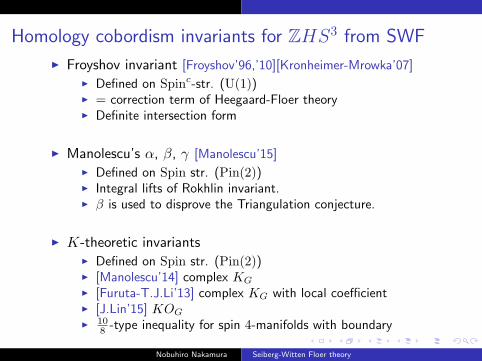
Homology cobordism invariants for ZHS3 from SWF

Froyshov invariant [Froyshov’96,’10][Kronheimer-Mrowka’07] Defined on Spinc-str. (U(1)) = correction term of Heegaard-Floer theory Definite intersection form

Manolescu’s α, β, γ [Manolescu’15] Defined on Spin str. (Pin(2)) Integral lifts of Rokhlin invariant. β is used to disprove the Triangulation conjecture.

K-theoretic invariants Defined on Spin str. (Pin(2)) [Manolescu’14] complex KG

[Furuta-T.J.Li’13] complex KG with local coefficient [J.Lin’15] KOG

108 -type inequality for spin 4-manifolds with boundary


Contents

Introduction

Overview (Casson inv & gauge theory)

Seiberg-Witten Floer stable homotopy type when b1 = 0

Homology cobordism invariants


Overview Casson invariant and gauge theory

Casson invariant λ(Y )

Y : ZHS3, Heegaard splitting Y = U0 ∪Σ U1

R(X) = π1X → SU(2)/conj ∼= SU(2)-flat connections/GR∗(X): irreducble part

R∗(U0)

zzR∗(Σ) R∗(Y )

dd

zzR∗(U1)

dd

Roughly λ(Y ) =1

2#(R∗(U0) ∩R∗(U1))


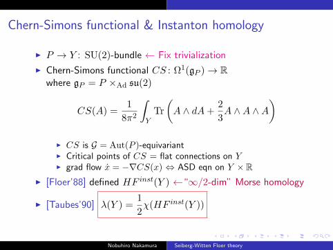
Chern-Simons functional & Instanton homology

P → Y : SU(2)-bundle ← Fix trivialization

Chern-Simons functional CS : Ω1(gP )→ Rwhere gP = P ×Ad su(2)

CS(A) =1

8π2

∫YTr

(A ∧ dA+

2

3A ∧A ∧A

) CS is G = Aut(P )-equivariant Critical points of CS = flat connections on Y grad flow x = −∇CS(x) ⇔ ASD eqn on Y × R

[Floer’88] defined HF inst(Y ) ←“∞/2-dim” Morse homology

[Taubes’90] λ(Y ) =1

2χ(HF inst(Y ))


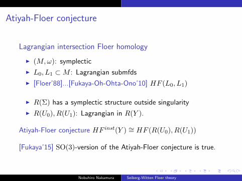
Atiyah-Floer conjecture

Lagrangian intersection Floer homology

(M,ω): symplectic

L0, L1 ⊂M : Lagrangian submfds

[Floer’88]...[Fukaya-Oh-Ohta-Ono’10] HF (L0, L1)

R(Σ) has a symplectic structure outside singularity

R(U0), R(U1): Lagrangian in R(Y ).

Atiyah-Floer conjecture HF inst(Y ) ∼= HF (R(U0), R(U1))

[Fukaya’15] SO(3)-version of the Atiyah-Floer conjecture is true.


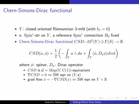
Chern-Simons-Dirac functional

Y : closed oriented Riemannian 3-mfd (with b1 = 0)

s: Spinc-str on Y , a reference Spinc connection B0 fixed

Chern-Simons-Dirac functional CSD : iΩ1(Y )⊕ Γ(S)→ R

CSD(a, ϕ) =1

2

(−∫Ya ∧ da+

∫Y⟨ϕ,Daϕ⟩dvol

)where ϕ: spinor, Da: Dirac operator

CSD is G = Map(Y,U(1))-equivariant ∇CSD = 0 ⇔ SW eqn on (Y, s) grad flow x = −∇CSD(x) ⇔ SW eqn on Y × R


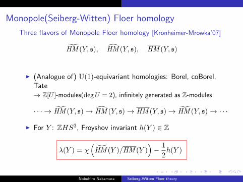
Monopole(Seiberg-Witten) Floer homology

Three flavors of Monopole Floer homology [Kronheimer-Mrowka’07]

HM (Y, s), HM (Y, s), HM (Y, s)

(Analogue of) U(1)-equivariant homologies: Borel, coBorel,Tate→ Z[U ]-modules(degU = 2), infinitely generated as Z-modules

· · · →

HM (Y, s)→ HM (Y, s)→ HM (Y, s)→

HM (Y, s)→ · · ·

For Y : ZHS3, Froyshov invariant h(Y ) ∈ Z

λ(Y ) = χ(

HM (Y )/HM (Y ))− 1

2h(Y )


Atiyah-Floer conjecture for SWF?

2-dim SW eqn = vortex equation→ moduli spaceM(Σ) = Sym•(Σ).

M(U0)

yySym•(Σ) M(Y )

dd

zzM(U1)

ee

(Not studied yet...???)


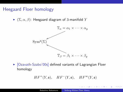
Heegaard Floer homology

(Σ, α, β): Heegaard diagram of 3-manifold Y

Tα = α1 × · · · × αg

vvSymg(Σ)

Tβ = β1 × · · · × βg

hh

[Ozavath-Szabo’00s] defined variants of Lagrangian Floerhomology

HF+(Y, s), HF−(Y, s), HF∞(Y, s)


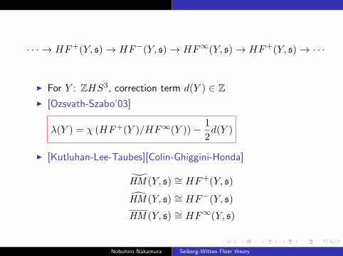
· · · → HF+(Y, s)→ HF−(Y, s)→ HF∞(Y, s)→ HF+(Y, s)→ · · ·

For Y : ZHS3, correction term d(Y ) ∈ Z [Ozsvath-Szabo’03]

λ(Y ) = χ (HF+(Y )/HF∞(Y ))− 1

2d(Y )

[Kutluhan-Lee-Taubes][Colin-Ghiggini-Honda]

HM (Y, s) ∼= HF+(Y, s)

HM (Y, s) ∼= HF−(Y, s)

HM (Y, s) ∼= HF∞(Y, s)


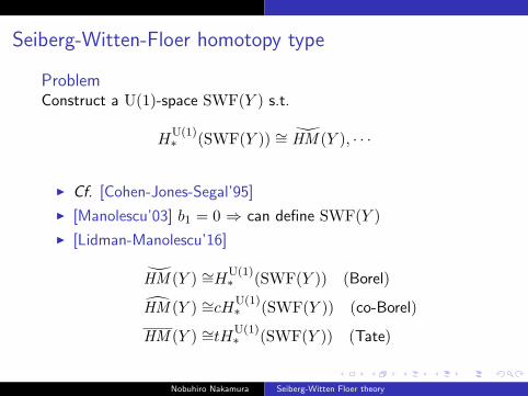
Seiberg-Witten-Floer homotopy type

ProblemConstruct a U(1)-space SWF(Y ) s.t.

HU(1)∗ (SWF(Y )) ∼=

HM (Y ), · · ·

Cf. [Cohen-Jones-Segal’95]

[Manolescu’03] b1 = 0 ⇒ can define SWF(Y )

[Lidman-Manolescu’16]

HM (Y ) ∼=HU(1)∗ (SWF(Y )) (Borel)

HM (Y ) ∼=cHU(1)∗ (SWF(Y )) (co-Borel)

HM (Y ) ∼=tHU(1)∗ (SWF(Y )) (Tate)


Idea of the construction of SWF(Y )

Finite dimensional approximation of CSD

Conley index


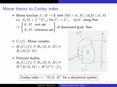
Morse theory to Conley index

Morse function f : M → R with ∂M = ∂+M ∪ ∂0M ∪ ∂−Ms.t. ∂±M = f−1(C±) for C− < C+, ∂0M : along flow

⇒

∂−M : exit set

∂+M : entrance set

of downward grad. flow

C∗(f): Morse complex

⇒ H∗(C∗(f)) ∼= H∗(M,∂−M) ∼=H∗(M/∂−M).

Poincare dualityH∗(C∗(f)) ∼= H∗(M,∂−M) ∼=H∗(M,∂+M) = H∗(C∗(−f)).

Conley index → “M/∂−M” for a dynamical system


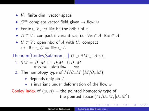
V : finite dim. vector space

C∞ complete vector field given → flow φ

For x ∈ V , let Rx be the oribit of x.

A ⊂ V : compact invariant set, i.e. ∀x ∈ A, Rx ⊂ A.

U ⊂ V : open nbd of A with U : compacts.t. Rx ⊂ U ⇒ Rx ⊂ A

Theorem[Conley,Salamon,...] U ⊃ ∃M ⊃ A s.t.

1. ∂M = ∂+Mentrance

∪ ∂0Malong flow

∪ ∂−Mexit

2. The homotopy type of M/∂−M (M/∂+M)

depends only on A is invariant under deformation of the flow φ

Conley index of (φ,A) = the pointed homotopy type ofthe pointed space (M/∂−M, [∂−M ])


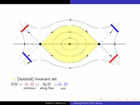
A: (isolated) invariant set∂M = ∂+M

entrance∪ ∂0M

along flow∪ ∂−M

exit


Finite dimensional approximation of CSD

CSD : iΩ1(Y )⊕ Γ(S)→ R, G-equivariant G = Map(Y,U(1)) = G0 ×H1(Y ;Z)×U(1) where

G0 =eif∣∣∣∣ f : Y → R,

∫Yfdvol = 0

← contractible

G0 ×H1(Y ;Z)-action on iΩ1(Y )⊕ Γ(S) is free.

the slice of G0-action: V = i ker d∗ ⊕ Γ(S)

Suppose b1(Y ) = 0 ⇒ G = G0 ×U(1), CSD: G-invariant

CSD with G-action ↔ CSD|V with U(1)-action

x = −∇(CSD|V)(x) ← U(1)-equivariant

[Fact] A =∪(bounded trajectries) ← invariant set

b1(Y ) = 0 ⇒ ∃ball ⊃ A


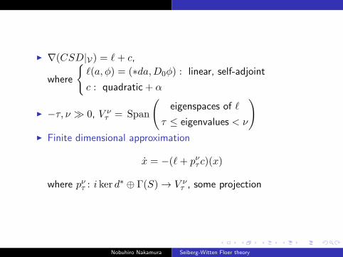
∇(CSD|V) = ℓ+ c,

where

ℓ(a, ϕ) = (∗da,D0ϕ) : linear, self-adjoint

c : quadratic+ α

−τ, ν ≫ 0, V ντ = Span

(eigenspaces of ℓ

τ ≤ eigenvalues < ν

) Finite dimensional approximation

x = −(ℓ+ pντ c)(x)

where pντ : i ker d∗ ⊕ Γ(S)→ V ν

τ , some projection


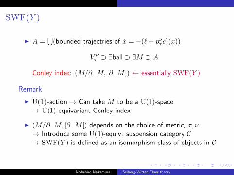
SWF(Y )

A =∪(bounded trajectries of x = −(ℓ+ pντ c)(x))

V ντ ⊃ ∃ball ⊃ ∃M ⊃ A

Conley index: (M/∂−M, [∂−M ]) ← essentially SWF(Y )

Remark

U(1)-action → Can take M to be a U(1)-space→ U(1)-equivariant Conley index

(M/∂−M, [∂−M ]) depends on the choice of metric, τ, ν.→ Introduce some U(1)-equiv. suspension category C→ SWF(Y ) is defined as an isomorphism class of objects in C


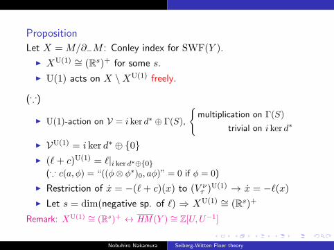
Proposition

Let X = M/∂−M : Conley index for SWF(Y ).

XU(1) ∼= (Rs)+ for some s.

U(1) acts on X \XU(1) freely.

(∵)

U(1)-action on V = i ker d∗ ⊕ Γ(S),

multiplication on Γ(S)

trivial on i ker d∗

VU(1) = i ker d∗ ⊕ 0 (ℓ+ c)U(1) = ℓ|i ker d∗⊕0

(∵ c(a, ϕ) = “((ϕ⊗ ϕ∗)0, aϕ)” = 0 if ϕ = 0)

Restriction of x = −(ℓ+ c)(x) to (V ντ )

U(1) → x = −ℓ(x) Let s = dim(negative sp. of ℓ) ⇒ XU(1) ∼= (Rs)+

Remark: XU(1) ∼= (Rs)+ ↔ HM (Y ) ∼= Z[U,U−1]


A definition of Froyshov invariant

Y : QHS3 with Spinc-structure

[Froyshov invariant] δU(1)(Y ) = −h(Y ) ∈ QδU(1)(Y ): Manolescu’s convention

h(Y ): Froyshov, Kronheimer-Mrowka

X = M/∂−M : Conley ind. for SWF(Y ), XU(1) ∼= (Rs)+.

Apply H∗U(1)( · ;F) (F: field) to the inclusion i : XU(1) → X

i∗ : H∗U(1)(X;F)→ H∗

U(1)(XU(1);F)

Note H∗+sU(1)(X

U(1)) ∼=Thom iso.

H∗U(1)(pt)

∼= F[u], deg u = 2.

Via this identification, ∃d, Im i∗ = ⟨ud⟩.

δU(1)(Y ) = −h(Y ) = d+ (some grading shift)


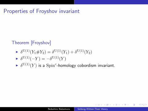
Properties of Froyshov invariant

Theorem [Froyshov]

δU(1)(Y1#Y2) = δU(1)(Y1) + δU(1)(Y2)

δU(1)(−Y ) = −δU(1)(Y )

δU(1)(Y ) is a Spinc-homology cobordism invariant.


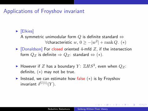
Applications of Froyshov invariant

[Elkies]A symmetric unimodular form Q is definite standard ⇔

∀characteristic w, 0 ≥ −|w2|+ rankQ. (∗) [Donaldson] For closed oriented 4-mfd Z, if the intersection

form QZ is definite ⇒ QZ : standard ⇔ (∗).

However if Z has a boundary Y : ZHS3, even when QZ :definite, (∗) may not be true.

Instead, we can estimate how false (∗) is by Froyshovinvariant δU(1)(Y ).


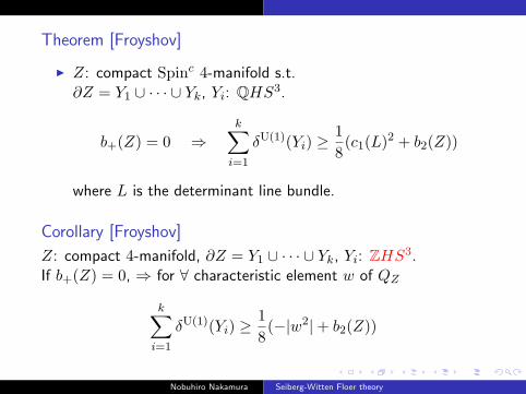
Theorem [Froyshov]

Z: compact Spinc 4-manifold s.t.∂Z = Y1 ∪ · · · ∪ Yk, Yi: QHS3.

b+(Z) = 0 ⇒k∑

i=1

δU(1)(Yi) ≥1

8(c1(L)

2 + b2(Z))

where L is the determinant line bundle.

Corollary [Froyshov]

Z: compact 4-manifold, ∂Z = Y1 ∪ · · · ∪ Yk, Yi: ZHS3.If b+(Z) = 0, ⇒ for ∀ characteristic element w of QZ

k∑i=1

δU(1)(Yi) ≥1

8(−|w2|+ b2(Z))


Proof of Froyshov’s theorem Y0, Y1: QHS3 with Spinc

Xi: Conley ind. for SWF(Yi) (i = 0, 1) Z: cobordism from Y0 to Y1 ∂Z = (−Y0) ∪ Y1 [Manolescu][T.Khandhawit] monopole map for cobordism→ Finite dim approx

f : Σ•X0 → Σ•X1 ← U(1)-map

We have a diagram

Σ•X0f−−−−→ Σ•X1x x

(Σ•X0)U(1)

∼=−−−−−−−−→if b+(Z) = 0

(Σ•X1)U(1)

Apply H∗U(1)( · )


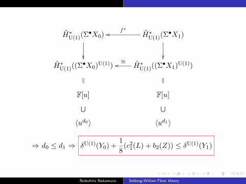
H∗U(1)(Σ

•X0)

H∗U(1)(Σ

•X1)f∗

oo

H∗

U(1)((Σ•X0)

U(1))

∥

H∗U(1)((Σ

•X1)U(1))

∼=oo

∥

F[u]∪ F[u]∪⟨ud0⟩ ⟨ud1⟩

⇒ d0 ≤ d1 ⇒ δU(1)(Y0) +1

8(c21(L) + b2(Z)) ≤ δU(1)(Y1)


Spin structure

On Spin structure, Seiberg-Witten Floer theory has aPin(2)-symmetry Pin(2) = U(1) ∪ jU(1) ⊂ Sp(1) ⊂ H

In fact, G = Pin(2)-action on ker d∗ ⊕ Γ(S) is givenon Γ(S) by multiplication

on ker d∗ via Pin(2)→ ±1, j 7→ −1⇒ ℓ+ c: G-equivariant

We obtain SWF(Y ) with G-action whose X satisfies XU(1) ∼= (Rs)+ where R = (Pin(2)→ ±1 R) G acts freely on X \XU(1)

For a spin cobordism Z from Y0 to Y1, we have G-equivariantfinite dim approx

f : Σ•X0 → Σ•X1


Manolescu’s α, β, γ

[Fact]

H∗G(pt;F2) = H∗(BG;F2) = F2[q, v]/(q

3)

where deg q = 1, deg v = 4(∵ G→ SU(2)→ RP2 → BG→ B SU(2) ∼= HP∞)

Apply H∗G( · ;F2) to the inclusion (Rs)+ ∼= XU(1) i→ X

H∗G(X)

i∗→ H∗G(X

U(1)) ∼= H∗G((Rs)+) ∼=

Thom iso.H∗

G(pt;F2)

im i∗ can be identified with an ideal J ⊂ F2[q, v]/(q3)

J has a form (va, qvb, q2vc) for a ≥ b ≥ c ≥ 0


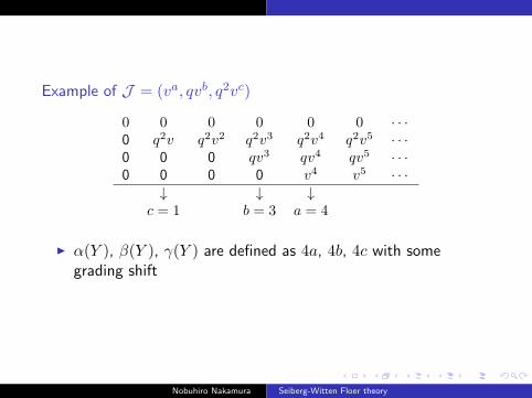
Example of J = (va, qvb, q2vc)

0 0 0 0 0 0 · · ·0 q2v q2v2 q2v3 q2v4 q2v5 · · ·0 0 0 qv3 qv4 qv5 · · ·0 0 0 0 v4 v5 · · ·

↓ ↓ ↓c = 1 b = 3 a = 4

α(Y ), β(Y ), γ(Y ) are defined as 4a, 4b, 4c with somegrading shift


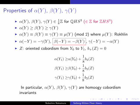
Properties of α(Y ), β(Y ), γ(Y )

α(Y ), β(Y ), γ(Y ) ∈ 18Z for QHS3 (∈ Z for ZHS3)

α(Y ) ≥ β(Y ) ≥ γ(Y )

α(Y ) ≡ β(Y ) ≡ γ(Y ) ≡ µ(Y ) (mod 2) where µ(Y ): Rokhlin

α(−Y ) = −γ(Y ), β(−Y ) = −β(Y ) , γ(−Y ) = −α(Y )

Z: oriented cobordism from Y0 to Y1, b+(Z) = 0

α(Y1) ≥α(Y0) +1

8b2(Z)

β(Y1) ≥β(Y0) +1

8b2(Z)

γ(Y1) ≥γ(Y0) +1

8b2(Z)

In particular, α(Y ), β(Y ), γ(Y ) are homoogy cobordisminvariants


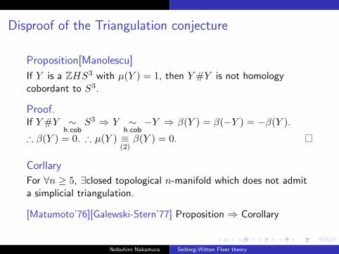
Disproof of the Triangulation conjecture

Proposition[Manolescu]

If Y is a ZHS3 with µ(Y ) = 1, then Y#Y is not homologycobordant to S3.

Proof.If Y#Y ∼

h.cobS3 ⇒ Y ∼

h.cob−Y ⇒ β(Y ) = β(−Y ) = −β(Y ).

∴ β(Y ) = 0. ∴ µ(Y ) ≡(2)

β(Y ) = 0.

Corllary

For ∀n ≥ 5, ∃closed topological n-manifold which does not admita simplicial triangulation.

[Matumoto’76][Galewski-Stern’77] Proposition ⇒ Corollary


Applications by Stoffregen

[Stoffregen’15] studies α, β, γ for connected sums of QHS3,especially Seifert fibered spaces

Theorem[Stoffregen’15]

The integral homology cobordism group θ3H contains a Z∞

summand generated by

Σ(p, 2p− 1, 2p+ 1), p ≥ 3, p : odd

Cf. [Furuta’90](p=2, q=3), [Fintushel-Stern’90]

Σ(p, q, pqn− 1), n ≥ 1, p, q : relatively prime

are linearly independent in θ3H


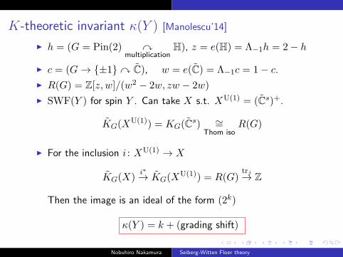
K-theoretic invariant κ(Y ) [Manolescu’14]

h = (G = Pin(2) multiplication

H), z = e(H) = Λ−1h = 2− h

c = (G→ ±1 C), w = e(C) = Λ−1c = 1− c.

R(G) = Z[z, w]/(w2 − 2w, zw − 2w)

SWF(Y ) for spin Y . Can take X s.t. XU(1) = (Cs)+.

KG(XU(1)) = KG(Cs) ∼=

Thom isoR(G)

For the inclusion i : XU(1) → X

KG(X)i∗→ KG(X

U(1)) = R(G)trj→ Z

Then the image is an ideal of the form (2k)

κ(Y ) = k + (grading shift)


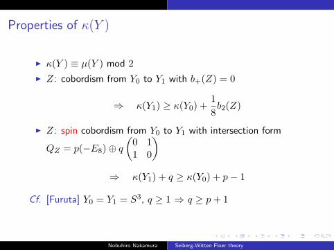
Properties of κ(Y )

κ(Y ) ≡ µ(Y ) mod 2

Z: cobordism from Y0 to Y1 with b+(Z) = 0

⇒ κ(Y1) ≥ κ(Y0) +1

8b2(Z)

Z: spin cobordism from Y0 to Y1 with intersection form

QZ = p(−E8)⊕ q

(0 11 0

)⇒ κ(Y1) + q ≥ κ(Y0) + p− 1

Cf. [Furuta] Y0 = Y1 = S3, q ≥ 1 ⇒ q ≥ p+ 1


Other versions of K-theoretic invariants

[Furuta-T.J.Li’13] complex KG with local coefficient

[J.Lin’15] KOG


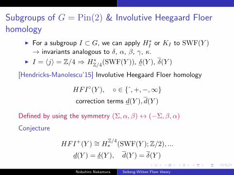
Subgroups of G = Pin(2) & Involutive Heegaard Floerhomology

For a subgroup I ⊂ G, we can apply H∗I or KI to SWF(Y )

→ invariants analogous to δ, α, β, γ, κ.

I = ⟨j⟩ = Z/4 ⇒ H∗Z/4(SWF(Y )), δ(Y ), δ(Y )

[Hendricks-Manolescu’15] Involutive Heegaard Floer homology

HFI(Y ), ∈ ,+,−,∞correction terms d(Y ), d(Y )

Defined by using the symmetry (Σ, α, β)↔ (−Σ, β, α)

Conjecture

HFI+(Y ) ∼= HZ/4∗ (SWF(Y );Z/2), ...

d(Y ) = δ(Y ), d(Y ) = δ(Y )


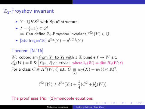
Z2-Froyshov invariant

Y : QHS3 with Spinc-structure

I = ±1 ⊂ S1

⇒ Can define Z2-Froyshov invariant δZ2(Y ) ∈ Q [Stoffregen’16] δZ2(Y ) = δU(1)(Y )

Theorem [N.’16]

W : cobordism from Y0 to Y1 with a Z bundle ℓ→W s.t.bℓ+(W ) = 0 & ℓ|Y0 , ℓ|Y1 : trivial where b(W ) = dimH(W ; ℓ)

For a class C ∈ H2(W ; ℓ) s.t. C ≡(2)

w2(X) + w1(ℓ⊗ R)2,

δZ2(Y1) ≥ δZ2(Y0) +1

4(C2 + bℓ2(W ))

The proof uses Pin−(2)-monopole equations


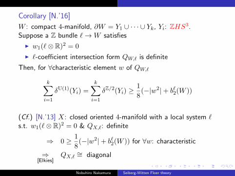
Corollary [N.’16]

W : compact 4-manifold, ∂W = Y1 ∪ · · · ∪ Yk, Yi: ZHS3.Suppose a Z bundle ℓ→W satisfies

w1(ℓ⊗ R)2 = 0

ℓ-coefficient intersection form QW,ℓ is definite

Then, for ∀characteristic element w of QW,ℓ

k∑i=1

δU(1)(Yi) =

k∑i=1

δZ/2(Yi) ≥1

8(−|w2|+ bℓ2(W ))

(Cf.) [N.’13] X: closed oriented 4-manifold with a local system ℓs.t. w1(ℓ⊗ R)2 = 0 & QX,ℓ: definite

⇒ 0 ≥ 1

8(−|w2|+ bℓ2(W )) for ∀w: characteristic

⇒[Elkies]

QX,ℓ∼= diagonal


Recent development of Seiberg-Witten Floer Theoryshimizu/Nakamura_f.pdf · 2017-02-01 · Recent...

Documents

Transcript of Recent development of Seiberg-Witten Floer Theoryshimizu/Nakamura_f.pdf · 2017-02-01 · Recent...