ELLIPTIC SPECTRA, THE WITTEN GENUS AND THE THEOREM …
67
ELLIPTIC SPECTRA, THE WITTEN GENUS AND THE THEOREM OF THE CUBE M. ANDO, M. J. HOPKINS, AND N. P. STRICKLAND Contents 1. Introduction 2 1.1. Outline of the paper 6 2. More detailed results 7 2.1. The algebraic geometry of even periodic ring spectra 7 2.2. Constructions of elliptic spectra 9 2.3. The complex-orientable homology of BU 2k for k ≤ 3 10 2.4. The complex-orientable homology of MU 2k for k ≤ 3 14 2.5. The σ–orientation of an elliptic spectrum 18 2.6. The Tate curve 20 2.7. The elliptic spectrum K Tate and its σ-orientation 23 2.8. Modularity 25 3. Calculation of C k ( b G a , G m ) 26 3.1. The cases k = 0 and k =1 26 3.2. The strategy for k = 2 and k =3 26 3.3. The case k =2 27 3.4. The case k = 3: statement of results 28 3.5. Additive cocycles 30 3.6. Multiplicative cocycles 32 3.7. The Weil pairing: cokernel of δ × :C 2 ( b G a , G m ) →C 3 ( b G a , G m ) 35 3.8. The map δ × :C 1 ( b G a , G m ) →C 2 ( b G a , G m ) 39 3.9. Rational multiplicative cocycles 40 4. Topological calculations 40 4.1. Ordinary cohomology 41 4.2. The isomorphism for BU 0 and BU 2 41 4.3. The isomorphism for rational homology and all k 42 4.4. The ordinary homology of BSU 42 4.5. The ordinary homology of BU 6 43 4.6. BSU and BU 6 for general E 46 Appendix A. Additive cocycles 48 A.1. Rational additive cocycles 48 1
Transcript of ELLIPTIC SPECTRA, THE WITTEN GENUS AND THE THEOREM …
ELLIPTIC SPECTRA, THE WITTEN GENUS AND THE THEOREM OF THECUBE
M. ANDO, M. J. HOPKINS, AND N. P. STRICKLAND
Contents
1. Introduction 2
1.1. Outline of the paper 6
2. More detailed results 7
2.1. The algebraic geometry of even periodic ring spectra 7
2.2. Constructions of elliptic spectra 9
2.3. The complex-orientable homology of BU〈2k〉 for k ≤ 3 10
2.4. The complex-orientable homology of MU〈2k〉 for k ≤ 3 14
2.5. The σ–orientation of an elliptic spectrum 18
2.6. The Tate curve 20
2.7. The elliptic spectrum KTate and its σ-orientation 23
2.8. Modularity 25
3. Calculation of Ck(Ga,Gm) 26
3.1. The cases k = 0 and k = 1 26
3.2. The strategy for k = 2 and k = 3 26
3.3. The case k = 2 27
3.4. The case k = 3: statement of results 28
3.5. Additive cocycles 30
3.6. Multiplicative cocycles 32
3.7. The Weil pairing: cokernel of δ× : C2(Ga,Gm) →C3(Ga,Gm) 35
3.8. The map δ× : C1(Ga,Gm) →C2(Ga,Gm) 39
3.9. Rational multiplicative cocycles 40
4. Topological calculations 40
4.1. Ordinary cohomology 41
4.2. The isomorphism for BU〈0〉 and BU〈2〉 41
4.3. The isomorphism for rational homology and all k 42
4.4. The ordinary homology of BSU 42
4.5. The ordinary homology of BU〈6〉 43
4.6. BSU and BU〈6〉 for general E 46
Appendix A. Additive cocycles 48
A.1. Rational additive cocycles 481
2 M. ANDO, M. J. HOPKINS, AND N. P. STRICKLAND
A.2. Divisibility 49
A.3. Additive cocycles: The modular case 51
Appendix B. Generalized elliptic curves 53
B.1. Examples of Weierstrass curves 58
B.2. Elliptic curves over C 60
B.3. Singularities 61
B.4. The cubical structure for the line bundle I(0) on a generalized elliptic curve 61
References 65
1. Introduction
This paper is part of a series ([HMM98, HM98] and other work in progress) getting at somenew aspects of the topological approach to elliptic genera. Most of these results were announcedin [Hop95].
In [Och87] Ochanine introduced the elliptic genus—a cobordism invariant of oriented mani-folds taking its values in the ring of (level 2) modular forms. He conjectured and proved half ofthe rigidity theorem—that the elliptic genus is multiplicative in bundles of spin manifolds withconnected structure group.
Ochanine defined his invariant strictly in terms of characteristic classes, and the question ofdescribing the elliptic genus in more geometric terms naturally arose—especially in connectionwith the rigidity theorem.
In [Wit87, Wit88] Witten interpreted Ochanine’s invariant in terms of index theory on loopspaces and offered a proof of the rigidity theorem. Witten’s proof was made mathematicallyrigorous by Bott and Taubes [BT89], and since then there have been several new proofs of therigidity theorem [Liu95, Ros98].
In the same papers Witten described a variant of the elliptic genus now known as the Wittengenus. There is a characteristic class λ of Spin manifolds, twice which is the first Pontrjagin class,p1. The Witten genus is a cobordism invariant of Spin-manifolds for which λ = 0, and it takesits values in modular forms (of level 1). It has exhibited a remarkably fecund relationship withgeometry (see [Seg88], and [HBJ92]).
Rich as it is, the theory of the Witten genus is not as developed as are the invariants described bythe index theorem. One thing that is missing is an understanding of the Witten genus of a family.Let S be a space, and Ms a family of n-dimensional Spin-manifolds (with λ = 0) parameterizedby the points of S. The family Ms defines an element in the cobordism group
MO〈8〉−nS,
where MO〈8〉 denotes the cobordism theory of “Spin-manifolds with λ = 0.” The Witten genusof this family should be some kind of “family of modular forms” parameterized by the points ofS. Motivated by the index theorem, we should regard this family of modular forms as an elementin
E−nS
for some (generalized) cohomology theory E. From the topological point of view, the Witten genusof a family is thus a multiplicative map of generalized cohomology theories
MO〈8〉 −→ E,
ELLIPTIC SPECTRA 3
and the question arises as to which E to choose, and how, in this language, to express the modularinvariance of the Witten genus. One candidate for E, elliptic cohomology, was introduced byLandweber, Ravenel, and Stong in [LRS95].
To keep the technicalities to a minimum, we focus in this paper on the restriction of the Wittengenus to stably almost complex manifolds with a trivialization of the Chern classes c1 and c2 ofthe tangent bundle. The bordism theory of such manifolds is denoted MU〈6〉. We will considergeneralized cohomology theories (or, more precisely, homotopy commutative ring spectra) E whichare even and periodic. In the language of generalized cohomology, this means that the cohomologygroups
E0(Sn)
are zero for n odd, and that for each pointed space X, the map
E0(S2) ⊗E0(pt)
E0(X) −→ E0(S2 ∧X)
is an isomorphism. In the language of spectra the conditions are that
πoddE = 0
and that π2E contains a unit. Our main result is a convenient description of all multiplicativemaps
MU〈6〉 −→ E.
In another paper in preparation we will give, under more restrictive hypotheses on E, an analogousdescription of the multiplicative maps
MO〈8〉 −→ E.
These results lead to a useful homotopy theoretic explanation of the Witten genus, and to anexpression of the modular invariance of the Witten genus of a family. To describe them it isnecessary to make use of the language of formal groups.
The assumption that E is even and periodic implies that the cohomology ring
E0CP∞.
is the ring of functions on a formal group PE over π0E = E0(pt) [Qui69, Ada74]. From the pointof view of the formal group, the result [Ada74, Part II, Lemma 4.6] can be interpreted as sayingthat the set of multiplicative maps
MU −→ E
is naturally in one to one correspondence with the set of rigid sections of a certain rigid line bundleΘ1(L) over PE . Here a line bundle is said to be rigid if it has a specified trivialization at the zeroelement, and a section is said to be rigid if it takes the specified value at zero. Our line bundleL is the one whose sections are functions that vanish at zero, or in other words L = O(−0).The fiber of Θ1(L) at a point a ∈ PE is defined to be L0 ⊗ L∗a; it is immediate that Θ1(L) has acanonical rigidification.
Similarly, given a line bundle L over a commutative group A, let Θ3(L) be the line bundle overA3 whose fiber at (a, b, c) is
Θ3(L)(a,b,c) =La+bLb+cLa+cL0
La+b+cLaLbLc.
In this expression the symbol “+” refers to the group law of A, and multiplication and divisionindicate the tensor product of lines and their duals. A cubical structure on L is a nowhere vanishingsection s of Θ3(L) satisfying (after making the appropriate canonical identifications of line bundles)
(rigid) s(0, 0, 0) = 1(symmetry) s(aσ(1), aσ(2), aσ(3)) = s(a1, a2, a3)(cocycle) s(b, c, d)s(a, b + c, d) = s(a + b, c, d)s(a, b, d).
4 M. ANDO, M. J. HOPKINS, AND N. P. STRICKLAND
(See [Bre83], and Remark 2.42 for comparison of conventions.) Our main result (2.50) asserts thatthe set of multiplicative maps
MU〈6〉 −→ E
is naturally in one to one correspondence with the set of cubical structures on L = O(−0).We have chosen a computational approach to the proof of this theorem partly because it is
elementary, and partly because it leads to a general result. In [AS98], the first and third authorsgive a less computational proof of this result (for formal groups of finite height in positive charac-teristic), using ideas from [Mum65, Gro72, Bre83] on the algebraic geometry of biextensions andcubical structures.
On an elliptic curve the line bundle O(−0) has a unique cubical structure. Indeed, for fixed xand y, there is by Abel’s theorem a rational function f(x, y, z) with divisor −x−y+0−−x−−y. Any two such functions have a constant ratio, so the quotient s(x, y, z) = f(x, y, 0)/f(x, y, z)is well-defined and is easily seen to determine a trivialization of Θ3(O(−0)). Since the onlyglobal functions on an elliptic curve are constants, the requirement s(0, 0, 0) = 1 determines thesection uniquely, and shows that it satisfies the “symmetry” and “cocycle” conditions. In fact the“theorem of the cube” (see for example [Mum70]) shows more generally that any line bundle overany abelian variety has a unique cubical structure.
Over the complex numbers, a transcendental formula for f(x, y, z) is
σ(x + y + z)σ(z)σ(x + y)σ(x + z)
,
where σ is the Weierstrass σ function. It follows that the unique cubical structure is given by
σ(x + y)σ(x + z)σ(y + z)σ(0)σ(x + y + z)σ(x)σ(y)σ(z)
. (1.1)
Putting all of this together, if the formal group PE can be identified with the formal completionof an elliptic curve, then there is a canonical multiplicative map
MU〈6〉 −→ E
corresponding to the unique cubical structure which extends to the elliptic curve.
Definition 1.2. An elliptic spectrum consists of
i. an even, periodic, homotopy commutative ring spectrum E with formal group PE over π0E;ii. a generalized elliptic curve C over E0(pt);iii. an isomorphism t : PE −→ C of PE with the formal completion of C.
For an elliptic spectrum E = (E,C, t), the σ-orientation
σE : MU〈6〉 −→ E
is the map corresponding to the unique cubical structure extending to C.
Note that this definition involves generalized elliptic curves over arbitrary rings. The relevanttheory is developed in [KM85, DR73]; we give a summary in Appendix B.
A map of elliptic spectra E1 = (E1, C1, t1) −→ E2 = (E2, C2, t2) consists of a map f : E1 −→ E2
of multiplicative cohomology theories, together with an isomorphism of elliptic curves
(π0f)∗C2 −→ C1,
ELLIPTIC SPECTRA 5
extending the induced map of formal groups. Given such a map, the uniqueness of cubical struc-tures over elliptic curves shows that
MU〈6〉σE1
wwww
wwww
w σE2
##GGGG
GGGG
G
E1f
// E2
(1.3)
commutes. We will refer to the commutativity of this diagram as the modular invariance of theσ-orientation.
By way of illustration, let’s consider examples derived from elliptic curves over C, and ordinarycohomology (for which the formal group is the additive group).
An elliptic curve over C is of the form C/Λ for some lattice Λ ⊂ C. The map of formal groupsderived from
C −→ C/Λ
gives an isomorphism tΛ, from the additive formal group to the formal completion of the ellipticcurve. Let RΛ be the graded ring C[uΛ, u−1
Λ ] with |uΛ| = 2, and define an elliptic spectrumHΛ = (EΛ, CΛ, tΛ) by taking EΛ to be the spectrum representing
H∗(− ;RΛ),
CΛ the elliptic curve C/Λ, and tΛ the isomorphism described above.
The abelian group of cobordism classes of 2n-dimensional stably almost complex manifolds witha trivialization of c1 and c2 is
MU〈6〉2n(pt).
The σ-orientation for HΛ thus associates to each such M , an element of (EΛ)2n(pt) which can bewritten
Φ(M ; Λ) · unΛ,
with
Φ(M ; Λ) ∈ C.
Suppose that Λ′ ⊂ C is another lattice, and that λ is a non-zero complex number for whichλ · Λ = Λ′. Then multiplication by λ gives an isomorphism C/Λ −→ C/Λ′. This extends to a mapHΛ′ −→ HΛ, of elliptic spectra, which, in order to induce the correct map of formal groups, mustsend uΛ′ to λuΛ (this is explained in example 2.3). The modular invariance of the σ-orientationthen leads to the equation
Φ(M ;λ · Λ) = λ−nΦ(M ; Λ).
This can be put in a more familiar form by choosing a basis for the lattice Λ. Given a complexnumber τ with positive imaginary part, let Λ(τ) be the lattice generated by 1 and τ , and set
f(M, τ) = Φ(M, Λ(τ)).
Given (a bc d
)∈ SL2(Z)
set
Λ = Λ(τ)
Λ′ = Λ ((a τ + b)/(c τ + d))
λ = (c τ + d)−1.
6 M. ANDO, M. J. HOPKINS, AND N. P. STRICKLAND
The above equation then becomes
f(M ; (a τ + b)/(c τ + d)) = (c τ + d)nf(M ; τ),
which is the functional equation satisfied by a modular form of weight n. It can be shown thatf(M, τ) is a holomorphic function of τ by considering the elliptic spectrum derived from the familyof elliptic curves
H× C/〈1, τ〉 −→ H
parameterized by the points of the upper half plane H, and with underlying homology theory
H∗(− ;O[u, u−1]
),
where O is the ring of holomorphic functions on H. Thus the σ-orientation associates a modularform of weight n to each 2n-dimensional MU〈6〉-manifold. Using an elliptic spectrum constructedout of K-theory and the Tate curve, one can also show that the modular forms that arise in thismanner have integral q-expansions (see §2.8).
In fact, it follows from formula (1.1) (for details see §2.7) that the q-expansion of this modularform is the Witten genus of M . The σ-orientation can therefore be viewed as a topologicalrefinement of the Witten genus, and its modular invariance (1.3), an expression of the modularinvariance of the Witten genus of a family.
All of this makes it clear that one can deduce special properties of the Witten genus by takingspecial choices of E. But it also suggests that the really natural thing to do is to consider allelliptic curves at once. This leads to some new torsion companions to the Witten genus, some newcongruences on the values of the Witten genus, and to the ring of topological modular forms. Itis the subject of the papers [HMM98, HM98].
1.1. Outline of the paper. In §2, we state our results and the supporting definitions in moredetail. In §2.3 we give a detailed account of our algebraic model for E0BU〈2k〉. In §2.4 we describeour algebraic model for E0MU〈2k〉. We deduce our results about MU〈2k〉 from the results aboutBU〈2k〉 and careful interpretation of the Thom isomorphism; the proof of the main result aboutE0BU〈2k〉 (Theorem 2.29) is the subject of §4.
In §2.5 we give in more detail the argument sketched in the introduction that there is a uniquecubical structure on any elliptic curve. We give an argument with explicit formulae which workswhen the elliptic curves in question are allowed to degenerate to singular cubics (“generalizedelliptic curves”), and also gives some extra insight even in the non-degenerate case. The proof ofthe main formula (Proposition 2.55) is given in appendix B.
In §2.6, we give a formula for the cubical structure on the Tate curve, inspired by the tran-scendental formula involving the σ-function that was mentioned in the introduction. In §2.7, weinterpret this formula as describing the σ-orientation for the elliptic spectrum KTate, and we showthat its effect on homotopy rings is the Witten genus. In §2.8, we deduce the modularity of theWitten genus from the modular invariance of the σ-orientation.
The rest of the main body of the paper assembles a proof of Theorem 2.29. In §3 we study aset Ck(Ga,Gm)(R) of formal power series in k variables over a ring R with certain symmetry andcocycle properties. This is a representable functor of R, in other words Ck(Ga,Gm) is an affinegroup scheme. For 0 ≤ k ≤ 3 we will eventually identify Ck(Ga,Gm) with spec(H∗BU〈2k〉). Fork = 3 we use a small fragment of the theory of Weil pairings associated to cubical structures; thisforms the heart of an alternative proof of our results [AS98] which works for p-divisible formalgroups but not for the formal group of an arbitrary generalized elliptic curve.
In §4 we first check that our algebraic model coincides with the usual description of spec(E0BU).We then compare our algebraic calculations to the homology of the fibration
BSU −→ BU −→ CP∞
to show that spec(H∗BSU) ∼= C2(Ga,Gm).
ELLIPTIC SPECTRA 7
We then recall Singer’s analysis of the Serre spectral sequence of the fibration
K(Z, 3) −→ BU〈6〉 −→ BSU.
By identifying the even homology of K(Z, 3) with the scheme of Weil pairings described in §3.7,we show that spec(H∗BU〈6〉) ∼= C3(Ga,Gm). Finally we deduce Theorem 2.29 for all E from thecase of ordinary homology.
The paper has two appendices. The first proves some results about the group of additivecocycles Ck(Ga, Ga)(A), which are used in §3. The second gives an exposition of the theory ofgeneralized elliptic curves, culminating in a proof of Proposition 2.55. We have tried to makethings as explicit as possible rather than relying on the machinery of algebraic geometry, and wehave given a number of examples.
2. More detailed results
2.1. The algebraic geometry of even periodic ring spectra. Let BU〈2k〉 → Z×BU be the(2k−1)–connected cover, and let MU〈2k〉 be the associated bordism theory. For an even periodicring spectrum E and for k ≤ 3, the map
RingSpectra(MU〈2k〉, E) −→ Algπ0E(E0MU〈2k〉, π0E)
is an isomorphism. In other words, the multiplicative maps MU〈2k〉 → E are in one-to-onecorrespondence with π0E-valued points of spec(π0E∧MU〈2k〉). If E is an elliptic spectrum, thenthe Theorem of the Cube endows this scheme with a canonical point. In order to connect thetopology to the algebraic geometry, we shall express some facts about even periodic ring spectrain the language of algebraic geometry.
2.1.1. Formal schemes and formal groups. Following [DG70], we will think of an affine scheme asa representable covariant functor from rings to sets. The functor (co-)represented by a ring A isdenoted spec A. The ring (co-)representing a functor X will be denoted OX .
A formal scheme is a filtered colimit of affine schemes. For example, the functor A1 associatingto a ring R its set of nilpotent elements is the colimit of the schemes spec(Z[x]/xk) and thus is aformal scheme.
The category of formal schemes has finite products: if X = colim Xα and Y = colimYβ thenX × Y = colim Xα × Yβ . The formal schemes in this paper will all be of the form An × Z =A1 × . . .× A1 × Z for some affine scheme Z. If X = colimα Xα is a formal scheme, then we shallwrite OX for limαOXα ; in particular we have ObA1 = Z[[x]]. We write ⊗ for the completed tensorproduct, so that for example
OX×Y = OX⊗OY .
If X → S is a morphism of schemes with a section j : S → X, then X will denote the completionof X along the section. Explicitly, the section j defines an augmentation
OXj∗−→ OS .
If J denotes the kernel of j∗, then
X = colimN
spec(OX/JN ).
For example, the zero element defines a section spec(Z) → A1, and the completion of A1 alongthis section is the formal scheme A1.
A commutative one-dimensional formal group over S is a commutative group G in the categoryof formal schemes over S which, locally on S, is isomorphic to S × A1 as a pointed formal schemeover S. We shall often omit “commutative” and “one-dimensional”, and simply refer to G as aformal group.
8 M. ANDO, M. J. HOPKINS, AND N. P. STRICKLAND
We shall use the notation Ga for the additive group, and Gm for the multiplicative group. Asfunctors we have Ga(R) = R and Gm(R) = R×. Thus Ga is the additive formal group, and Ga(R)is the additive group of nilpotent elements of R.
If the group scheme Gm acts on a scheme X, we have a map α : Gm ×X → X, correspondingto a map α∗ : OX −→ OGm×X = OX [u, u−1]. We put (OX)n = f | α(f) = unf. This makes OX
into a graded ring.
A graded ring R∗ is said to be of finite type over Z if each Rn is a finitely generated abeliangroup.
2.1.2. Even ring spectra and schemes. If E is an even periodic ring spectrum, then we write
SEdef= spec(π0E).
If X is a space, we write E0X and E0X for the unreduced E-(co)homology of X. If A is aspectrum, we write E0A and E0A for its spectrum (co)homology. These are related by the formulaE0X = E0Σ∞X+.
Let X be a CW-complex. If Xα is the set of finite subcomplexes of X then we write XE
for the formal scheme colimα spec(E0Xα). This gives a covariant functor from spaces to formalschemes over SE .
We say that X is even if H∗X is a free abelian group, concentrated in even degrees. If X is evenand E is an even periodic ring spectrum, then E0X is a free module over E0, and E0X is its dual.The restriction to even spaces of the functor X 7→ XE preserves finite products. For example thespace P
def= CP∞ is even, and PE is (non-canonically) isomorphic to the formal affine line. Themultiplication P × P → P classifying the tensor product of line bundles makes the scheme PE
into a (one-dimensional commutative) formal group over SE .
The formal group PE is not quite the same as the one introduced by Quillen [Qui69]. The ringof functions on Quillen’s formal group is E∗(P ), while the ring of functions on PE is E0(P ). Thehomogeneous parts of E∗(P ) can interpreted as sections of line bundles over PE . For example, letI be the ideal of functions on PE which vanish along the identity section. The natural map
I/I2 → E0(S2) = π2E (2.1)
is an isomorphism. Now I/I2 is, by definition, the Zariski cotangent space to the group PE at theidentity, and defines a line bundle over specπ0E. This line bundle is customarily denoted ω, andcan be regarded as the sheaf of invariant 1-forms on PE . In this way we will identify π2E withinvariant 1-forms on PE . More generally, π2nE can be identified with the module of sections ofωn (i.e., invariant differentials of degree n on PE).
Note that for any space X, the map
E0(X)⊗π0E π−2n(E) −→ E2n(X)
is an isomorphism, and so E2n(X) can be identified with the module of sections of the pull-backof the line bundle ω−n to XE .
Let E be an even ring spectrum, which need not be periodic. Let EP =∨
n∈ZΣ2nE. There isan evident way to make this into a commutative ring spectrum with the property that π∗EP =E∗[u, u−1] with u ∈ π2EP . With this structure, EP becomes an even periodic ring spectrum.Note that when X is finite we just have EP 0X =
⊕n E2nX, so the ring EP 0X has a natural
even grading. If X is an infinite, even CW-complex then EP 0X is the completed direct sum (withrespect to the topology defined by kernels of restrictions to finite subcomplexes) of the groupsE2nX and so again has a natural even grading.
We write HP for the 2-periodic integer Eilenberg-MacLane spectrum HZP , and MP forMUP = MU〈0〉. The formal group of HP is the additive group Ga; and we may choose anadditive coordinate z on Ga for which u = dz. By Quillen’s theorem [Qui69], the formal group ofMP is Lazard’s universal formal group law.
ELLIPTIC SPECTRA 9
If X is an even, homotopy commutative H-space, then XE is a (commutative but in generalnot one-dimensional) formal group. In that case E0X is a Hopf algebra over E0 and we writeXE = spec(E0X) for the corresponding group scheme. It is the Cartier dual of the formal groupXE . We recall (from [Dem72, §II.4], for example; see also [Str99a, Section 6.4] for a treatmentadapted to the present situation) that the Cartier dual of a formal group G is the functor fromrings to groups
Hom(G,Gm)(A) = (u, f) | u : spec(A) −→ S , f ∈ (Formal groups)(u∗G, u∗Gm).Let b ∈ E0X⊗E0X be the adjoint of the identity map E0X → E0X. Given a ring homomorphismg : E0X → A we get a map u : spec(A) → SE and an element g(b) ∈ (A⊗E0X)× = (A⊗OXE
)×,which corresponds to a map of schemes
f : u∗XE −→ u∗Gm.
One shows that it is a group homomorphism, and so gives a map of group schemes
XE −→ Hom(XE ,Gm), (2.2)
which turns out to be an isomorphism.
2.2. Constructions of elliptic spectra. Recall that an elliptic spectrum is a triple (E, C, t)consisting of an even, periodic, homotopy commutative ring spectrum E, a generalized ellipticcurve C over E0(pt), and an isomorphism formal groups
t : PE −→ C.
Here are some examples.
Example 2.3. As discussed in the introduction, if Λ ⊂ C is a lattice, then the quotient C/Λ isan elliptic curve CΛ over C. The covering map C → C/Λ gives an isomorphism tΛ : CΛ
∼= Ga.Let EΛ be the spectrum representing the cohomology theory H∗(− ;C[uΛ, u−1
Λ ]). Define HΛ tobe the elliptic spectrum (EΛ, CΛ, tΛ). Note that uΛ can be taken to correspond to the invariantdifferential dz on C under the isomorphism (2.1).
Given a non-zero complex number λ, consider the map
f : EλΛ −→ EΛ
uλΛ 7→ λuΛ
(i.e. π2f scales the invariant differential by λ). The induced map of formal groups is simplymultiplication by λ, and so extends to the isomorphism
CΛλ·−→ CλΛ
of elliptic curves. Thus f defines a map of elliptic spectra
f : HλΛ −→ HΛ.
Example 2.4. Let CHP be the cuspidal cubic curve y2z = x3 over spec(Z). In §B.1.4, we givean isomorphism s : (CHP )reg ∼= Ga and so s : CHP
∼= Ga = PHP . Thus the triple (HP,CHP , s) isan elliptic spectrum.
Example 2.5. Let C = CK be the nodal cubic curve y2z + xyz = x3 over spec(Z). In §B.1.4,we give an isomorphism t : (CK)reg ∼= Gm so CK
∼= Gm = PK . The triple (K, CK , t) is an ellipticspectrum.
Example 2.6. Let C/S be an untwisted generalized elliptic curve (see Definition B.2) with theproperty that the formal group C is Landweber exact (For example, this is automatic if OS is a Q-algebra). Landweber’s exact functor theorem gives an even periodic cohomology theory E∗(− ),together with an isomorphism of formal groups t : PE −→ C. This is the classical constructionof elliptic cohomology; and gives rise to many examples. In fact, the construction identifies arepresenting spectrum E up to canonical isomorphism, since Franke [Fra92] and Strickland [Str99a,Proposition 8.43] show that there are no phantom maps between Landweber exact elliptic spectra.
10 M. ANDO, M. J. HOPKINS, AND N. P. STRICKLAND
Example 2.7. In §2.6, we describe an elliptic spectrum based on the Tate elliptic curve, withunderlying spectrum K[[q]].
2.3. The complex-orientable homology of BU〈2k〉 for k ≤ 3. Let E be an even periodicring spectrum with a coordinate x ∈ E0P , giving rise to a formal group law F over E0. Letρ : P 3 → BU〈6〉 be the map (see (2.24)) such that the composition
P 3 ρ−→ BU〈6〉 → BU
classifies the virtual bundle∏
i(1 − Li). Let f = f(x1, x2, x3) be the power series which is theadjoint of E0ρ in the ring E0P 3⊗E0BU〈6〉 ∼= E0BU〈6〉[[x1, x2, x3]]. It is easy to check that fsatisfies the following three conditions.
f(x1, x2, 0) = 1 (2.8a)
f(x1, x2, x3) is symmetric in the xi (2.8b)
f(x1, x2, x3)f(x0, x1 +F x2, x3) = f(x0 +F x1, x2, x3)f(x0, x1, x3). (2.8c)
We will eventually prove the following result.
Theorem 2.9. E0BU〈6〉 is the universal example of an E0-algebra R equipped with a formalpower series f ∈ R[[x1, x2, x3]] satisfying the conditions (2.8).
In this section we will reformulate this statement (as the case k = 3 of Theorem 2.29) in a waywhich avoids the choice of a coordinate.
2.3.1. The functor Ck.
Definition 2.10. If A and T are abelian groups, we let C0(A, T ) be the group
C0(A, T ) def= (Sets)(A, T ),
and for k ≥ 1 we let Ck(A, T ) be the subgroup of f ∈ (Sets)(Ak, T ) such that
f(a1, . . . , ak−1, 0) = 0; (2.11a)
f(a1, . . . , ak) is symmetric in the ai; (2.11b)
f(a1, a2, a3, . . . , ak) + f(a0, a1 + a2, a3, . . . , ak) = f(a0 + a1, a2, a3, . . . , ak) + f(a0, a1, a3, . . . , ak).(2.11c)
We refer to (2.11c) as the cocycle condition for f . It really only involves the first two argumentsof f , with the remaining arguments playing a dummy role. Of course, because f is symmetric, wehave a similar equation for any pair of arguments of f .
Remark 2.12. We leave it to the reader to verify that the condition (2.11a) can be replaced withthe weaker condition
f(0, . . . , 0) = 0 (2.11a’)
Remark 2.13. Let Z[A] denote the group ring of A, and let I[A] be its augmentation ideal. Fork ≥ 0 let
Ck(A) def= SymkZ[A] I[A]
be the kth symmetric tensor power of I[A], considered as a module over the group ring. One hasC0(A) = Z[A] and C1(A) = I[A]. For k ≥ 1, the abelian group Ck(A) is the quotient of Symk
Z I[A]by the relation
([c]− [c + a1])⊗ ([0]− [a2])⊗ . . .⊗ ([0]− [ak]) = ([0]− [a1])⊗ ([c]− [c + a2])⊗ . . .⊗ ([0]− [ak])
for c ∈ A. After some rearrangement and reindexing, this relation may be expressed in terms ofgenerators of the form 〈a1, . . . , ak〉 def= ([0]− [a1])⊗ . . .⊗ ([0]− [ak]) by the formula
〈a1, a2, a3, . . . , ak〉 − 〈a0 + a1, a2, a3, . . . , ak〉+ 〈a0, a1 + a2, a3, . . . , ak〉 − 〈a0, a1, a3, . . . , ak〉 = 0.
ELLIPTIC SPECTRA 11
It follows that the map of sets
Ak → Ck(A)
(a1, . . . , ak) 7→ 〈a1, . . . , ak〉
induces an isomorphism
(Abelian groups)(Ck(A), T ) ∼= Ck(A, T ).
Remark 2.14. Definition 2.10 generalizes to give a subgroup Ck(A, B) of the group of mapsf : Ak −→ B, if A and B are abelian groups in any category with finite products.
Definition 2.15. If G and T are formal groups over a scheme S, and we wish to emphasize therole of S, we will write Ck
S(G,T ). For any ring R, we define
Ck(G,T )(R) = (u, f) | u : spec(R) −→ S , f ∈ Ckspec(R)(u
∗G, u∗T ).
This gives a covariant functor from rings to groups. We shall abbreviate Ck(G,Gm × S) toCk(G,Gm).
Remark 2.16. It is clear from the definition that, for all maps of schemes S′ → S, the naturalmap
Ck(G×S S′,Gm) → Ck(G,Gm)×S S′
is an isomorphism.
Proposition 2.17. Let G be a formal group over a scheme S. For all k, the functor Ck(G,Gm)is an affine commutative group scheme.
Proof. We assume that k > 0, leaving the modifications for the case k = 0 to the reader. Itsuffices to work locally on S, and so we may choose a coordinate x on G. Let F be the resultingformal group law of G. We let A be the set of multi-indices α = (α1, . . . , αk), where each αi
is a nonnegative integer. We define R = OS [bα | α ∈ A][b−10 ], and f(x1, . . . , xk) =
∑α bαxα ∈
R[[x1, . . . , xk]]. Thus, f defines a map spec(R)×S Gk −→ Gm, and in fact spec(R) is easily seen tobe the universal example of a scheme over S equipped with such a map. We define power seriesg0, . . . , gk by
gi =
i = 0 f(0, . . . , 0)i < k f(x1, . . . , xi−1, xi+1, xi, . . . , xk)f(x1, . . . , xk)−1
i = k f(x1, . . . , xk)f(x0 +F x1, x2, . . . )−1f(x0, x1 +F x2, . . . )f(x0, x1, x3, . . . )−1
We then let I be the ideal in R generated by all the coefficients of all the power series gi − 1. Itis not hard to check that spec(R/I) has the universal property that defines Ck(G,Gm).
Remark 2.18. A similar argument shows that Ck(G, T ) is a group scheme when T is a formalgroup, or when T is the additive group Ga.
Remark 2.19. If G is a formal group and k > 0 then the inclusion Ck(G, Gm) −→ Ck(G,Gm) isan isomorphism, so we shall not distinguish between these two schemes. Indeed, we can locallyidentify Ck(G,Gm)(R) with a set of power series f as in the above proof. One of the conditionson f is that f(0, . . . , 0) = 1, so when x1, . . . , xk are nilpotent we see that f(x1, . . . , xn) = 1 modnilpotents, so f(x1, . . . , xn) ∈ Gm ⊂ Gm. This does not work for k = 0, as then we have
C0(G,Gm) = Map(G,Gm) 6= Map(G, Gm) = C0(G, Gm).
12 M. ANDO, M. J. HOPKINS, AND N. P. STRICKLAND
2.3.2. The maps δ : Ck(G,T ) → Ck+1(G,T ). We now define maps of schemes that will turn outto correspond to the maps BU〈2k + 2〉 −→ BU〈2k〉 of spaces.
Definition 2.20. If G and T are abelian groups, and if f : Gk → T is a map of sets, then letδ(f) : Gk+1 → T be the map given by the formula
δ(f)(a0, . . . , ak) = f(a0, a2, . . . , ak) + f(a1, a2, . . . , ak)− f(a0 + a1, a2, . . . , ak). (2.21)
It is clear that δ generalizes to abelian groups in any category with products. We leave it tothe reader to verify the following.
Lemma 2.22. For k ≥ 1, the map δ induces a homomorphism of groups
δ : Ck(G,T ) → Ck+1(G, T ).
Moreover, if G and T are formal groups over a scheme S, then δ induces a homomorphism ofgroup schemes δ : Ck(G,T ) −→ Ck+1(G,T ).
Remark 2.23. When A and T are discrete abelian groups, the group H2(A; T ) def= cok(δ : C1(A, T ) −→C2(A, T )) classifies central extensions of A by T . The next map δ : C2(A, T ) −→ C3(A, T )) canalso be interpreted in terms of biextensions [Mum65, Gro72, Bre83].
2.3.3. Relation to BU〈2k〉. For any space X, we write K∗(X) for the periodic complex K-theorygroups of X; in the case of a point we have K∗ = Z[v, v−1] with v ∈ K−2. We have K2t(X) =[X,Z×BU ] for all t. We also consider the connective K-theory groups bu∗(X), so bu∗ = Z[v] andbu2t(X) = [X,BU〈2t〉]. To make this true when t = 0, we adopt the convention that BU〈0〉 = Z×BU . Multiplication by vt : Σ2tbu → bu gives an identification of the 0-space of Σ2tbu with BU〈2t〉.Under this identification, the projection BU〈2t + 2〉 −→ BU〈2t〉 is derived from multiplication byv mapping Σ2t+2bu → Σ2tbu.
For t ≥ 0 we define a map
ρt : P t = (CP∞)t → BU〈2t〉 (2.24)
as follows. The map ρ0 : P → 1 × BU ⊂ BU〈0〉 is just the map classifying the tautological linebundle L. For t > 0, let L1, . . . , L2 be the obvious line bundles over P t. Let xi ∈ bu2(P t) be thebu-theory Euler class, given by the formula
vxi = 1− Li.
Then we have the isomorphisms
bu∗(P t) ∼= Z[v][[x1, . . . , xt]]
K∗(P t) ∼= Z[v, v−1][[x1, . . . , xt]].
The class∏
i xi ∈ bu2t(P t) gives the map ρt. Note that the composition
P t ρt−→ BU〈2t〉 → BU
classifies the bundle∏
i(1− Li).
Since P and BU〈2t〉 are abelian group objects in the homotopy category of topological spaces,we can define
Ct(P,BU〈2t〉) ⊂ [P t, BU〈2t〉] = bu2t(P t).
Then we have the following.
Proposition 2.25. The map ρt is contained in the subgroup Ct(P,BU〈2t〉) of bu2t(P t) and sat-isfies
v∗ρt+1 = δ(ρt) ∈ Ct+1(P, BU〈2t〉).
ELLIPTIC SPECTRA 13
Proof. It suffices to check that ft gives an element of Ct(P, BU〈0〉). As the group structure of Pcorresponds to the tensor product of line bundles, while the group structure of BU〈0〉 correspondsto the Whitney sum of vector bundles, the cocycle condition (2.11c) amounts to the equation
(1− L2)(1− L3) + (1− L1)(1− L2L3) = (1− L1L2)(1− L3) + (1− L1)(1− L2)
in K0(P 3). The other conditions for membership in Ct are easily verified. Similarly, the equationv∗ρt+1 = δ(ρt) follows from the equation
(1− L1) + (1− L2)− (1− L1L2) = (1− L1)(1− L2).
Now let E be an even periodic ring spectrum. Applying E-homology to the map ρk gives ahomomorphism
E0ρk : E0Pk → E0BU〈2k〉.
For k ≤ 3, BU〈2k〉 is even ([Sin68] or see §4), and of course the same is true of P , and so we mayconsider the adjoint ρk of E0ρk in E0BU〈2k〉⊗E0P k. Proposition 2.25 then implies the following.
Corollary 2.26. The element ρk ∈ E0BU〈2k〉⊗E0P k is an element of Ck(PE ,Gm)(E0BU〈2k〉).
Definition 2.27. For k ≤ 3, let fk : BU〈2k〉E → Ck(PE ,Gm) be the map classifying the cocycleρk.
Corollary 2.28. The map fk is a map of group schemes. For k ≤ 2, the diagram
BU〈2k + 2〉E
fk+1
²²
vE// BU〈2k〉E
fk
²²
Ck+1(PE ,Gm)δ
// Ck(PE ,Gm)
commutes.
Proof. The commutativity of the diagram follows easily from the Proposition. To see that fk isa map of group schemes, note that the group structure on BU〈2k〉E is induced by the diagonalmap ∆: BU〈2k〉 −→ BU〈2k〉 ×BU〈2k〉. The commutative diagram
P k ∆−−−−→ P k × P k
ρk
yyρk×ρk
BU〈2k〉 ∆−−−−→ BU〈2k〉 ×BU〈2k〉shows that
BU〈2k〉E ×BU〈2k〉E −→ BU〈2k〉E
pulls the function ρk back to the multiplication of ρk ⊗ 1 and 1 ⊗ ρk as elements of the ringE0(BU〈2k〉2)⊗E0P k of functions on P k
E × (BU〈2k〉E × BU〈2k〉E). The result follows, since thegroup structure of Ck(PE ,Gm) is induced by the multiplication of functions in OP k
E.
Our main calculation, and the promised coordinate-free version of Theorem 2.9, is the following.
Theorem 2.29. For k ≤ 3, the map of group schemes
BU〈2k〉E fk−→ Ck(PE ,Gm)
is an isomorphism.
14 M. ANDO, M. J. HOPKINS, AND N. P. STRICKLAND
This is proved in §4. The cases k ≤ 1 are essentially well-known calculations. For k = 2and k = 3 we can reduce to the case E = MP , using Quillen’s theorem that π0MP carriesthe universal example of a formal group law. Using connectivity arguments and the Atiyah-Hirzebruch spectral sequence, we can reduce to the case E = HP . After these reductions, weneed to compare H∗BU〈2k〉 with OCk(bGa,Gm). We analyze H∗(BU〈2k〉;Q) and H∗(BU〈2k〉;Fp)using the Serre spectral sequence, and we analyze OCk(bGa,Gm) by direct calculation, one primeat a time. For the case k = 3 we also give a model for the scheme associated to the polyno-mial subalgebra of H∗(K(Z, 3);Fp), and by fitting everything together we show that the mapBU〈2k〉E −→ Ck(PE ,Gm) is an isomorphism.
Remark 2.30. As BU〈2k〉E = Hom(BU〈2k〉E ,Gm) = Ck(PE ,Gm), it is natural to hope thatone could
i. define a formal group scheme Ck(PE) which could be interpreted as the k’th symmetric tensorpower of the augmentation ideal in the group ring of the formal group PE ;
ii. show that Ck(PE ,Gm) = Hom(Ck(PE),Gm); andiii. prove that BU〈2k〉E = Ck(PE).
This would have advantages over the above theorem, because the construction X 7→ XE is functo-rial for all spaces and maps, whereas the construction X 7→ XE is only functorial for commutativeH-spaces and H-maps. It is in fact possible to carry out this program, at least for k ≤ 3. Itrelies on the apparatus developed in [Str99a], and the full strength of the present paper is requiredeven to prove that C3(G) (as defined by a suitable universal property) exists. Details will appearelsewhere.
2.4. The complex-orientable homology of MU〈2k〉 for k ≤ 3. We now turn our attention tothe Thom spectra MU〈2k〉. We first note that when k ≤ 3, the map BU〈2k〉 → BU〈0〉 = Z×BUis a map of commutative, even H-spaces. The Thom isomorphism theorem as formulated by[MR81] implies that E0MU〈2k〉 is an E0BU〈2k〉-comodule algebra; and a choice of orientationMU〈0〉 → E gives an isomorphism
E0MU〈2k〉 ∼= E0BU〈2k〉of comodule algebras. In geometric language, this means that the scheme MU〈2k〉E is a principalhomogeneous space or “torsor” for the group scheme BU〈2k〉E .
In this section, we work through the Thom isomorphism to describe the object which corre-sponds to MU〈2k〉E under the isomorphism BU〈2k〉E ∼= Ck(PE ,Gm) of Theorem 2.29. Whereasthe schemes BU〈2k〉E are related to functions on the formal group PE of E, the schemes MU〈2k〉Eare related to the sections of the ideal sheaf I(0) on PE . In §2.4.4, we describe the analogueCk(G; I(0)) for the line bundle I(0) of the functor Ck(G,Gm). In §2.4.5, we give the map
gk : MU〈2k〉E → Ck(PE ; I(0))
which is our description of MU〈2k〉E .
2.4.1. Torsors. We begin with a brief review of torsors in general and the Thom isomorphism inparticular.
Definition 2.31. Let S be a scheme and G a group scheme over S. A (right) G-torsor over S isan S-scheme X with a right action
X ×Gµ−→ X
of the group G, with the property that there exists a faithfully flat S-scheme T and an isomorphism
G× T −→ X × T
of T -schemes, compatible with the action of G×T . (All the products here are to be interpreted asfiber products over S.) Any such isomorphism is a trivialization of X over T . A map of G-torsorsis just an equivariant map of schemes. Note that a map of torsors is automatically an isomorphism.
ELLIPTIC SPECTRA 15
When G = spec(H) is affine over S = spec(A), a G-torsor works out to consists of an affineS-scheme T = spec(M) and a right coaction
Mµ∗−→ M ⊗A H
with the property that over some faithfully flat A-algebra B there is an isomorphism
H ⊗A B −→ M ⊗A B
of rings which is a map of right H ⊗A B-comodules.
For example, consider the relative diagonal
MU〈2k〉 ∆−→ MU〈2k〉 ∧BU〈2k〉+.
If E is an even periodic ring spectrum and k ≤ 3, then by the Kunneth and universal coefficienttheorems, the map ∆ induces an action
MU〈2k〉E ×BU〈2k〉E µ−→ MU〈2k〉E .
of the group scheme BU〈2k〉E on MU〈2k〉E . The scheme MU〈2k〉E is in fact a torsor for BU〈2k〉E .Indeed, a complex orientation MU〈0〉 −→ E restricts to an orientation Φ: MU〈2k〉 −→ E whichinduces an isomorphism
E0MU〈2k〉 ∆−→ E0MU〈2k〉 ∧BU〈2k〉+ Φ∧BU〈2k〉+−−−−−−−−→ E0BU〈2k〉+ (2.32)
of E0BU〈2k〉-comodule algebras.
2.4.2. The line bundle I(0). Another source of torsors is line bundles. If L is a line bundle(invertible sheaf of OX -modules) over X, let Γ×(L) be the functor of rings
Γ×(L)(R) = (u, s) | u : spec(R) −→ X , s a trivialization of u∗L.Then Γ×(L) is a Gm-torsor over X, and Γ× is an equivalence between the category of line bundles(and isomorphisms) and the category of Gm torsors. We will often not distinguish in notationbetween L and the associated Gm-torsor Γ×(L).
Let G be a formal group over a scheme S. The ideal sheaf I(0) associated to the zero sectionS ⊂ G defines a line bundle over G. Indeed, the set of global sections of I(0) is the set offunctions f ∈ OG such that f |S = 0. Locally on S, a choice of coordinate x gives an isomorphismOG = OS [[x]], and the module of sections is the ideal (x), which is free of rank 1.
If C is a generalized elliptic curve over, then we again let I(0) denote the ideal sheaf of S ⊂ C.Its restriction to the formal completion C is the same as the line bundle over C constructed above.
2.4.3. The Thom sheaf. Suppose that X is a finite complex and V is a complex vector bundle overX. We write XV for its Thom spectrum, with bottom cell in degree equal to the real rank of V .This is the suspension spectrum of the usual Thom space. Now let E be an even periodic ringspectrum. The E0X-module E0XV is the sheaf of sections of a line bundle over XE . We shallwrite L(V ) for this line bundle, and L defines a functor from vector bundles over X to line bundlesover XE . If V and W are two complex vector bundles over X then there is a natural isomorphism
L(V ⊕W ) ∼= L(V )⊗ L(W ), (2.33)
and so L extends to the category of virtual complex vector bundles by the formula L(V −W ) =L(V )⊗ L(W )−1. Moreover, if f : Y → X is a map of spaces, then there is a natural isomorphism(spec E0f)∗L(V ) ∼= L(f∗V ) of line bundles over YE . This construction extends naturally to infinitecomplexes by taking suitable (co)limits.
Example 2.34. For example, if L is the tautological line bundle over P = CP∞ then the zerosection P −→ PL induces an isomorphism E0PL ∼= E0P = ker(E0P −→ E0), and thus gives anisomorphism
L(L) ∼= I(0) (2.35)
of line bundles over PE .
16 M. ANDO, M. J. HOPKINS, AND N. P. STRICKLAND
2.4.4. The functors Θk (after Breen [Bre83]). We recall that the category of line bundles or Gm-torsors is a strict Picard category, or in other words a symmetric monoidal category in which everyobject L has an inverse L−1, and the twist map of L ⊗ L is the identity. This means that theprocedures we use below to define line bundles give results that are well-defined up to coherentcanonical isomorphism.
Suppose that G is a formal group over a scheme S and L is a line bundle over G.
Definition 2.36. A rigid line bundle over G is a line bundle L equipped with a specified trivi-alization of L|S at the identity S → G. A rigid section of such a line bundle is a section s whichextends the specified section at the identity. A rigid isomorphism between two rigid line bundlesis an isomorphism which preserves the specified trivializations.
Definition 2.37. Suppose that k ≥ 1. Given a subset I ⊆ 1, . . . , k, we define σI : GkS −→ G by
σI(a1, . . . , ak) =∑
i∈I ai, and we write LI = σ∗IL, which is a line bundle over GkS . We also define
the line bundle Θk(L) over GkS by the formula
Θk(L) def=⊗
I⊂1,...,k(LI)(−1)|I| . (2.38)
Finally, we define Θ0(L) = L.
For example we have
Θ0(L)a = La
Θ1(L)a =L0
La
Θ2(L)a,b =L0 ⊗ La+b
La ⊗ Lb
Θ3(L)a,b,c =L0 ⊗ La+b ⊗ La+c ⊗ Lb+c
La ⊗ Lb ⊗ Lc ⊗ La+b+c.
We observe three facts about these bundles.
i. Θk(L) has a natural rigid structure for k > 0.ii. For each permutation σ ∈ Σk, there is a canonical isomorphism
ξσ : π∗σΘk(L) ∼= Θk(L),
where πσ : GkS −→ Gk
S permutes the factors. Moreover, these isomorphisms compose in theobvious way.
iii. There is a canonical identification (of rigid line bundles over Gk+1S )
Θk(L)a1,a2,... ⊗Θk(L)−1a0+a1,a2,... ⊗Θk(L)a0,a1+a2,... ⊗Θk(L)−1
a0,a1,...∼= 1. (2.39)
Definition 2.40. A Θk–structure on a line bundle L over a group G is a trivialization s of theline bundle Θk(L) such that
i. for k > 0, s is a rigid section;ii. s is symmetric in the sense that for each σ ∈ Σk, we have ξσπ∗σs = s;iii. the section s(a1, a2, . . . )⊗s(a0+a1, a2, . . . )−1⊗s(a0, a1+a2, . . . )⊗s(a0, a1, . . . )−1 corresponds
to 1 under the isomorphism (2.39).
A Θ3–structure is known as a cubical structure [Bre83]. We write Ck(G;L) for the set of Θk-structures on L over G. Note that C0(G;L) is just the set of trivializations of L, and C1(G;L) isthe set of rigid trivializations of Θ1(L). We also define a functor from rings to sets by
Ck(G;L)(R) = (u, f) | u : spec(R) −→ S , f ∈ Ckspec(R)(u
∗G; u∗L).Remark 2.41. Note that for the trivial line bundle OG, the set Ck(G;OG) reduces to that of thegroup Ck(G,Gm) of cocycles introduced in §2.3.1.
ELLIPTIC SPECTRA 17
Remark 2.42. There are some differences between our functors Θk and Breen’s functors Λ andΘ [Bre83]. Let L′ = Θ1(L)−1 be the line bundle La/L0. Then there are natural isomorphisms
Λ(L′) ∼= Θ2(L)
Θ(L′) ∼= Θ3(L)−1.
Breen also uses the notation Θ1(M) for Θ(L′) [Bre83, Equation 2.8.1]. As the trivializations ofL biject with those of L−1 in an obvious way, our definition of cubical structures is equivalent toBreen’s.
Proposition 2.43. If G is a formal group over S, and L is a trivializable line bundle over G,then the functor Ck(G;L) is a scheme, whose formation commutes with change of base. Moreover,Ck(G;L) is a trivializable torsor for Ck(G,Gm).
Proof. There is an evident action of Ck(G,Gm) on Ck(G;L), and a trivialization of L clearly givesan equivariant isomorphism of Ck(G;L) with Ck(G;OG) = Ck(G,Gm). Given this, the Propo-sition follows from the corresponding statements for Ck(G,Gm), which were proved in Proposi-tion 2.17.
The following lemmas can easily be checked from Definitions 2.37 and 2.40.
Lemma 2.44. If L is a line bundle over a formal group G, then there is a canonical isomorphism
Θk(L)a0,a2,... ⊗Θk(L)a1,a2,... ⊗Θk(L)−1a0+a1,a2,...
∼= Θk+1(L)a0,...,ak.
Lemma 2.45. There is a natural map δ : Ck(G;L) −→ Ck+1(G;L), given by
δ(s)(a0, . . . , ak) = s(a0, a2, . . . )s(a1, a2, . . . )s(a0 + a1, a2, . . . )−1,
where the right hand side is regarded as a section of Θk+1(L) by the isomorphism of the previouslemma.
2.4.5. Relation to MU〈2k〉. For 1 ≤ i ≤ k, let Li be the line bundle over the i factor of P k. Recallfrom (2.24) that the map ρk : P k → BU〈2k〉 pulls the tautological virtual bundle over BU〈2k〉back to the bundle
V =⊗
i
(1− Li).
Passing to Thom spectra gives a map
(P k)V → MU〈2k〉which determines an element sk of E0MU〈2k〉⊗E0((P k)V ).
We recall from (2.35) that there is an isomorphism of line bundles L(L) ∼= I(0) over PE , whereI(0) is the ideal sheaf of the zero section; and that the functor L (from virtual vector bundles toline bundles over XE) sends direct sums to tensor products. Together these observations give anisomorphism
L(V ) ∼= Θk(I(0)) (2.46)
of line bundles over P kE . With this identification, sk is a section of the pull-back of Θk(I(0)) along
the projection MU〈2k〉E −→ SE .
Lemma 2.47. The section sk is a Θk-structure.
Proof. This is analogous to Corollary 2.26.
Let
MU〈2k〉E gk−→ Ck(PE ; I(0))
be the map classifying the Θk-structure sk. We note that the isomorphism BU〈2k〉E ∼= Ck(PE ,Gm)gives Ck(PE ; I(0)) the structure of a torsor for the group scheme BU〈2k〉E .
18 M. ANDO, M. J. HOPKINS, AND N. P. STRICKLAND
Theorem 2.48. For k ≤ 3, the map gk is a map of torsors for the group BU〈2k〉E (and so anisomorphism). Moreover, the map MU〈2k + 2〉 −→ MU〈2k〉 induces the map δ : Ck(PE ; I(0)) −→Ck+1(PE ; I(0)).
Proof. Let us write µ for the action
Ck(PE ; I(0))× Ck(PE ,Gm) −→ Ck(PE ; I(0)).
If funiv is the universal element of Ck(PE ,Gm) and suniv is the universal element of Ck(PE ; I(0)),then µ is characterized by the equation
µ∗suniv = funivsuniv, (2.49)
as elements of Ck(PE ; I(0))(OCk(PE ;I(0))×Ck(PE ,Gm)).
Now consider the commutative diagram
(P k)V ∆ //
²²
(P k)V ∧ (P k)+
²²
MU〈2k〉∆
// MU〈2k〉 ∧BU〈2k〉+.
Applying E-homology and then taking the adjoint in E0(BU〈2k〉+ ∧MU〈2k〉)⊗E0(P k)V gives asection of Θk(I(0)) over BU〈2k〉E ×MU〈2k〉E . The counterclockwise composition identifies thissection as the pull-back of the section sk under the action
MU〈2k〉E ×BU〈2k〉E ∆E
−−→ MU〈2k〉Eas in §2.4.1. Via the isomorphism BU〈2k〉E ∼= Ck(PE ,Gm) of Theorem 2.29, the clockwise com-position is funivsk. From the description of µ (2.49) it follows that gk is a map of torsors, asrequired.
Another diagram chase shows that the map MU〈2k + 2〉 −→ MU〈2k〉 is compatible with themap δ : Ck(GE ; I(0)) −→ Ck+1(GE ; I(0)).
Corollary 2.50. For 0 ≤ k ≤ 3, maps of ring spectra MU〈2k〉 −→ E are in bijective correspon-dence with Θk-structures on I(0) over GE.
Proof. Since E∗MU〈2k〉 is torsion free and concentrated in even degrees, one has
[MU〈2k〉, E] = E0MU〈2k〉 = Homπ0E(E0MU〈2k〉, π0E).
One checks that maps of ring spectra correspond to ring homomorphisms, so
RingSpectra(MU〈2k〉, E) = Algπ0E(E0MU〈2k〉, π0E).
This is just the set of global sections of MU〈2k〉E over SE , which is the set of Θk-structures onI(0) over GE by the theorem.
Example 2.51. Maps of ring spectra MP = MU〈0〉 −→ E are in bijective correspondence withglobal trivializations of the sheaf I(0) ∼= L(L), that is, with generators x of the augmentationideal E0P → E0(pt).
Example 2.52. Maps of ring spectra MU = MU〈2〉 → E are in bijective correspondence withrigid sections of ω ⊗ I(0)−1, or equivalently with rigid sections of ω−1 ⊗ I(0). The isomorphism(2.46) identifies sections of ω−1⊗I(0) with elements of E0(PL−1), and the rigid sections are thosewhich restrict to the identity under the inclusion
S0 → PL−1
of the bottom cell. It is equivalent to give a class x ∈ E2(P ) whose restriction to E2(S2) is thesuspension of 1 ∈ E0S0; this is the description of maps MU → E in [Ada74].
2.5. The σ–orientation of an elliptic spectrum.
ELLIPTIC SPECTRA 19
2.5.1. Elliptic spectra and the Theorem of the Cube. Let C be a generalized elliptic curve overan affine scheme S. To begin, note that the smooth locus Creg is a group scheme over S, so wecan define Θ3(I(0)) over Creg. We define a cubical structure on C to be a cubical structure onI(0)|Creg ; and we write C3(C; I(0)) for C3(Creg; I(0)).
Theorem 2.53. For any (nonsingular) elliptic curve C over a normal scheme S, there is a uniquecubical structure s(C/S) ∈ C3(C; I(0)). It has the following properties:
i. If C ′/S′ is obtained from C/S by base change along f : S′ −→ S, then
s(C ′/S′) = f∗s(C/S)
ii. If t : C ′ −→ C is an isomorphism over S, then
s(C ′/S) = (t3)∗s(C/S).
Proof. The first claim follows from [Gro72, Expose VIII, Cor. 7.5] (see also [Bre83, Proposition2.4]); the argument was sketched in the introduction. The other claims are immediate by unique-ness.
We would like to extend this to the case where S need not be normal and C is allowed to havesingularities. In this generality there may be many cubical structures (for example when C isa cuspidal cubic over spec(Z), with Creg = Ga) but nonetheless there will be a canonical choiceof one. To prove this, we will exhibit a formula which gives the unique cubical structure on theuniversal elliptic curve over Z[a1, a2, a3, a4, a6][∆−1] and give a density argument to show that thisformula works in general.
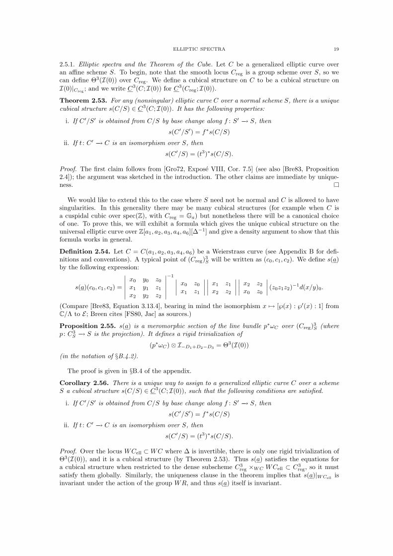
Definition 2.54. Let C = C(a1, a2, a3, a4, a6) be a Weierstrass curve (see Appendix B for defi-nitions and conventions). A typical point of (Creg)3S will be written as (c0, c1, c2). We define s(a)by the following expression:
s(a)(c0, c1, c2) =
∣∣∣∣∣∣
x0 y0 z0
x1 y1 z1
x2 y2 z2
∣∣∣∣∣∣
−1 ∣∣∣∣x0 z0
x1 z1
∣∣∣∣∣∣∣∣
x1 z1
x2 z2
∣∣∣∣∣∣∣∣
x2 z2
x0 z0
∣∣∣∣ (z0z1z2)−1d(x/y)0.
(Compare [Bre83, Equation 3.13.4], bearing in mind the isomorphism x 7→ [℘(x) : ℘′(x) : 1] fromC/Λ to E ; Breen cites [FS80, Jac] as sources.)
Proposition 2.55. s(a) is a meromorphic section of the line bundle p∗ωC over (Creg)3S (wherep : C3
S −→ S is the projection). It defines a rigid trivialization of
(p∗ωC)⊗ I−D1+D2−D3 = Θ3(I(0))
(in the notation of §B.4.2).
The proof is given in §B.4 of the appendix.
Corollary 2.56. There is a unique way to assign to a generalized elliptic curve C over a schemeS a cubical structure s(C/S) ∈ C3(C; I(0)), such that the following conditions are satisfied.
i. If C ′/S′ is obtained from C/S by base change along f : S′ −→ S, then
s(C ′/S′) = f∗s(C/S)
ii. If t : C ′ −→ C is an isomorphism over S, then
s(C ′/S) = (t3)∗s(C/S).
Proof. Over the locus WCell ⊂ WC where ∆ is invertible, there is only one rigid trivialization ofΘ3(I(0)), and it is a cubical structure (by Theorem 2.53). Thus s(a) satisfies the equations fora cubical structure when restricted to the dense subscheme C3
reg ×WC WCell ⊂ C3reg, so it must
satisfy them globally. Similarly, the uniqueness clause in the theorem implies that s(a)|WCell isinvariant under the action of the group WR, and thus s(a) itself is invariant.
20 M. ANDO, M. J. HOPKINS, AND N. P. STRICKLAND
Now suppose we have a generalized elliptic curve C over a general base S. At least locally, wecan choose a Weierstrass parameterization of C and then use the formula s(a) to get a cubicalstructure. Any other Weierstrass parameterization is related to the first one by the action of WR,so it gives the same cubical structure by the previous paragraph. We can thus patch togetherour local cubical structures to get a global one. The stated properties follow easily from theconstruction.
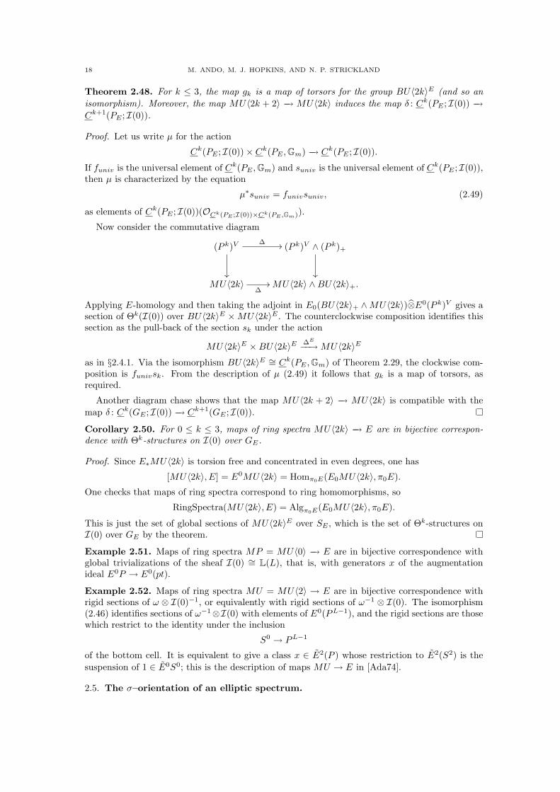
Theorem 2.57. For any elliptic spectrum E = (E, C, t) there is a canonical map of ring spectra
σE : MU〈6〉 −→ E.
This map is natural in the sense that if f : E −→ E′ = (E′, C ′, t′) is a map of elliptic spectra, thenthe diagram
MU〈6〉σE
xxxx
xxxx
x σE′
##GGGG
GGGG
G
Ef
// E′
commutes (up to homotopy).
Proof. This is now very easy. Let s(C/SE) be the cubical structure constructed in Corollary 2.56,and let s(C/SE) be the restriction of s(C/S) to CE . The orientation is the map σE : MU〈6〉 −→ E
corresponding to t∗s(C/S) via Corollary 2.50. The functoriality follows from the functoriality ofs in the corollary.
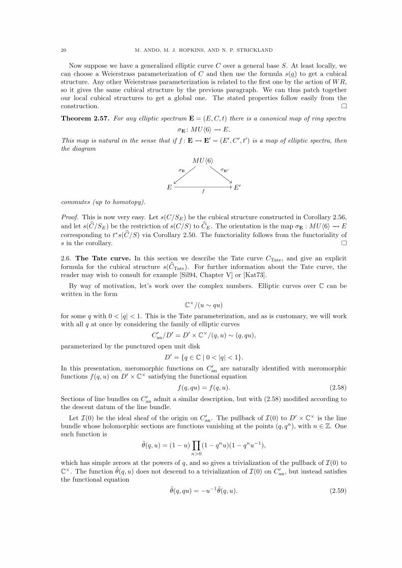
2.6. The Tate curve. In this section we describe the Tate curve CTate, and give an explicitformula for the cubical structure s(CTate). For further information about the Tate curve, thereader may wish to consult for example [Sil94, Chapter V] or [Kat73].
By way of motivation, let’s work over the complex numbers. Elliptic curves over C can bewritten in the form
C×/(u ∼ qu)
for some q with 0 < |q| < 1. This is the Tate parameterization, and as is customary, we will workwith all q at once by considering the family of elliptic curves
C ′an/D′ = D′ × C×/(q, u) ∼ (q, qu),
parameterized by the punctured open unit disk
D′ = q ∈ C | 0 < |q| < 1.In this presentation, meromorphic functions on C ′an are naturally identified with meromorphicfunctions f(q, u) on D′ × C× satisfying the functional equation
f(q, qu) = f(q, u). (2.58)
Sections of line bundles on C ′an admit a similar description, but with (2.58) modified according tothe descent datum of the line bundle.
Let I(0) be the ideal sheaf of the origin on C ′an. The pullback of I(0) to D′ × C× is the linebundle whose holomorphic sections are functions vanishing at the points (q, qn), with n ∈ Z. Onesuch function is
θ(q, u) = (1− u)∏n>0
(1− qnu)(1− qnu−1),
which has simple zeroes at the powers of q, and so gives a trivialization of the pullback of I(0) toC×. The function θ(q, u) does not descend to a trivialization of I(0) on C ′an, but instead satisfiesthe functional equation
θ(q, qu) = −u−1θ(q, u). (2.59)
ELLIPTIC SPECTRA 21
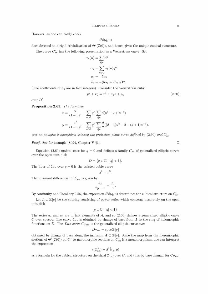
However, as one can easily check,
δ3θ(q, u)
does descend to a rigid trivialization of Θ3(I(0)), and hence gives the unique cubical structure.
The curve C ′an has the following presentation as a Weierstrass curve. Set
σk(n) =∑
d|ndk
αk =∑n>0
σk(n)qn
a4 = −5α3
a6 = −(5α3 + 7α5)/12
(The coefficients of a6 are in fact integers). Consider the Weierstrass cubic
y2 + xy = x3 + a4x + a6 (2.60)
over D′.
Proposition 2.61. The formulae
x =u
(1− u)2+
∑n>0
qn∑
d|nd(ud − 2 + u−d)
y =u2
(1− u)3+
∑n>0
qn∑
d|n
d
2((d− 1)ud + 2− (d + 1)u−d).
give an analytic isomorphism between the projective plane curve defined by (2.60) and C ′an.
Proof. See for example [Sil94, Chapter V §1].
Equation (2.60) makes sense for q = 0 and defines a family Can of generalized elliptic curvesover the open unit disk
D = q ∈ C | |q| < 1.The fiber of Can over q = 0 is the twisted cubic curve
y2 = x3.
The invariant differential of Can is given bydx
2y + x=
du
u.
By continuity and Corollary 2.56, the expression δ3θ(q, u) determines the cubical structure on Can.
Let A ⊂ Z[[q]] be the subring consisting of power series which converge absolutely on the openunit disk
q ∈ C | |q| < 1 .
The series a4 and a6 are in fact elements of A, and so (2.60) defines a generalized elliptic curveC over spec A. The curve Can is obtained by change of base from A to the ring of holomorphicfunctions on D. The Tate curve CTate is the generalized elliptic curve over
DTate = specZ[[q]]
obtained by change of base along the inclusion A ⊂ Z[[q]]. Since the map from the meromorphicsections of Θ3(I(0)) on C3 to meromorphic sections on C3
an is a monomorphism, one can interpretthe expression
s(C3an) = δ3θ(q, u)
as a formula for the cubical structure on the sheaf I(0) over C, and thus by base change, for CTate.
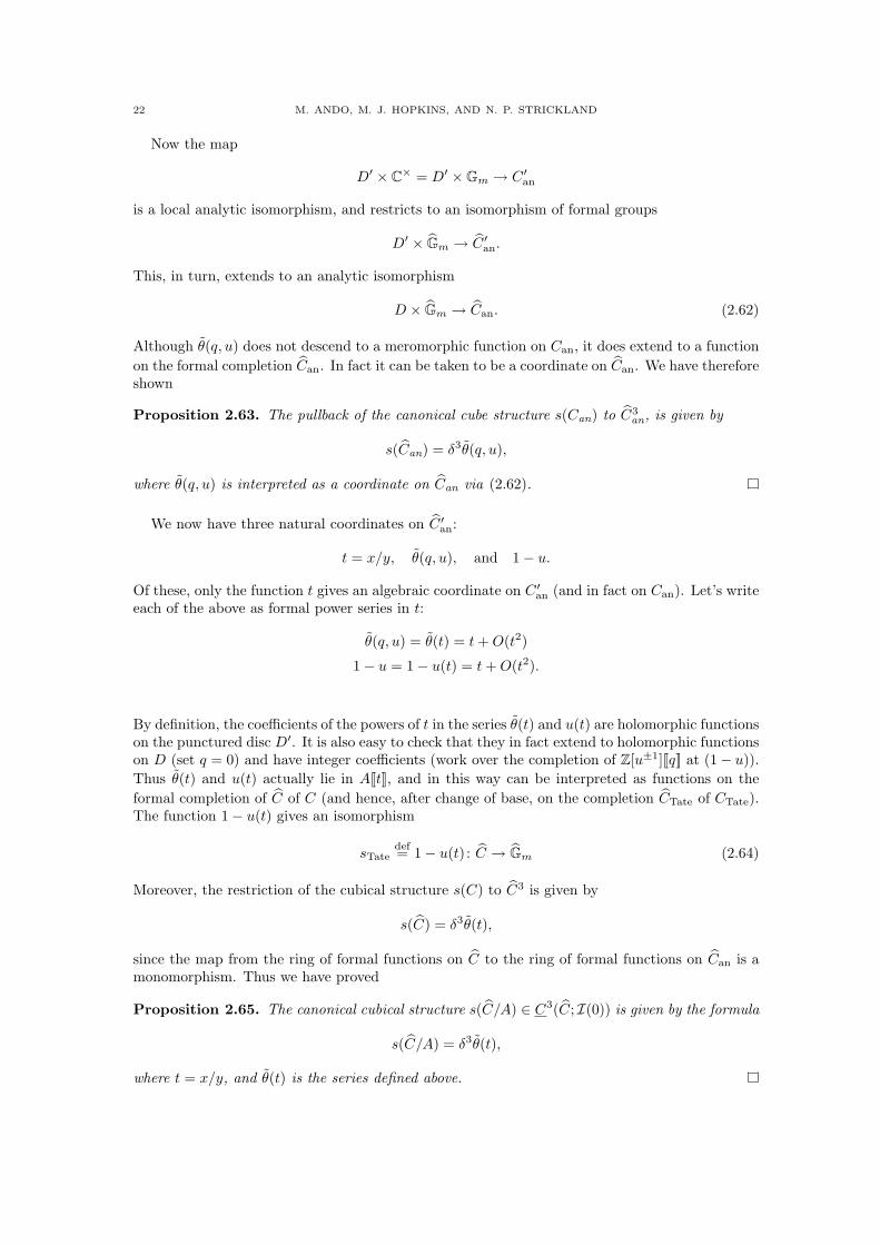
22 M. ANDO, M. J. HOPKINS, AND N. P. STRICKLAND
Now the map
D′ × C× = D′ ×Gm → C ′an
is a local analytic isomorphism, and restricts to an isomorphism of formal groups
D′ × Gm → C ′an.
This, in turn, extends to an analytic isomorphism
D × Gm → Can. (2.62)
Although θ(q, u) does not descend to a meromorphic function on Can, it does extend to a functionon the formal completion Can. In fact it can be taken to be a coordinate on Can. We have thereforeshown
Proposition 2.63. The pullback of the canonical cube structure s(Can) to C3an, is given by
s(Can) = δ3θ(q, u),
where θ(q, u) is interpreted as a coordinate on Can via (2.62).
We now have three natural coordinates on C ′an:
t = x/y, θ(q, u), and 1− u.
Of these, only the function t gives an algebraic coordinate on C ′an (and in fact on Can). Let’s writeeach of the above as formal power series in t:
θ(q, u) = θ(t) = t + O(t2)
1− u = 1− u(t) = t + O(t2).
By definition, the coefficients of the powers of t in the series θ(t) and u(t) are holomorphic functionson the punctured disc D′. It is also easy to check that they in fact extend to holomorphic functionson D (set q = 0) and have integer coefficients (work over the completion of Z[u±1][[q]] at (1− u)).Thus θ(t) and u(t) actually lie in A[[t]], and in this way can be interpreted as functions on theformal completion of C of C (and hence, after change of base, on the completion CTate of CTate).The function 1− u(t) gives an isomorphism
sTatedef= 1− u(t) : C → Gm (2.64)
Moreover, the restriction of the cubical structure s(C) to C3 is given by
s(C) = δ3θ(t),
since the map from the ring of formal functions on C to the ring of formal functions on Can is amonomorphism. Thus we have proved
Proposition 2.65. The canonical cubical structure s(C/A) ∈ C3(C; I(0)) is given by the formula
s(C/A) = δ3θ(t),
where t = x/y, and θ(t) is the series defined above.
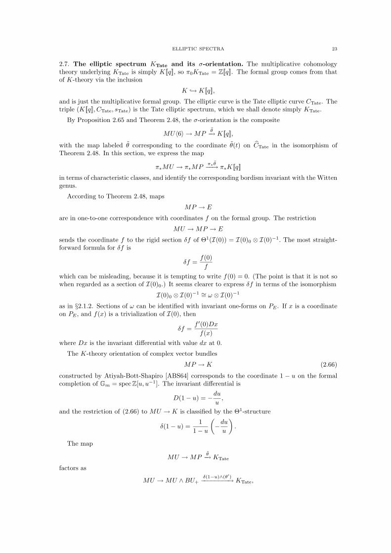
ELLIPTIC SPECTRA 23
2.7. The elliptic spectrum KTate and its σ-orientation. The multiplicative cohomologytheory underlying KTate is simply K[[q]], so π0KTate = Z[[q]]. The formal group comes from thatof K-theory via the inclusion
K → K[[q]],
and is just the multiplicative formal group. The elliptic curve is the Tate elliptic curve CTate. Thetriple (K[[q]], CTate, sTate) is the Tate elliptic spectrum, which we shall denote simply KTate.
By Proposition 2.65 and Theorem 2.48, the σ-orientation is the composite
MU〈6〉 → MPθ−→ K[[q]],
with the map labeled θ corresponding to the coordinate θ(t) on CTate in the isomorphism ofTheorem 2.48. In this section, we express the map
π∗MU → π∗MPπ∗θ−−→ π∗K[[q]]
in terms of characteristic classes, and identify the corresponding bordism invariant with the Wittengenus.
According to Theorem 2.48, maps
MP → E
are in one-to-one correspondence with coordinates f on the formal group. The restriction
MU → MP → E
sends the coordinate f to the rigid section δf of Θ1(I(0)) = I(0)0 ⊗ I(0)−1. The most straight-forward formula for δf is
δf =f(0)f
which can be misleading, because it is tempting to write f(0) = 0. (The point is that it is not sowhen regarded as a section of I(0)0.) It seems clearer to express δf in terms of the isomorphism
I(0)0 ⊗ I(0)−1 ∼= ω ⊗ I(0)−1
as in §2.1.2. Sections of ω can be identified with invariant one-forms on PE . If x is a coordinateon PE , and f(x) is a trivialization of I(0), then
δf =f ′(0)Dx
f(x)where Dx is the invariant differential with value dx at 0.
The K-theory orientation of complex vector bundles
MP → K (2.66)
constructed by Atiyah-Bott-Shapiro [ABS64] corresponds to the coordinate 1 − u on the formalcompletion of Gm = specZ[u, u−1]. The invariant differential is
D(1− u) = −du
u,
and the restriction of (2.66) to MU → K is classified by the Θ1-structure
δ(1− u) =1
1− u
(−du
u
).
The map
MU → MPθ−→ KTate
factors as
MU → MU ∧BU+δ(1−u)∧(θ′)−−−−−−−−→ KTate,
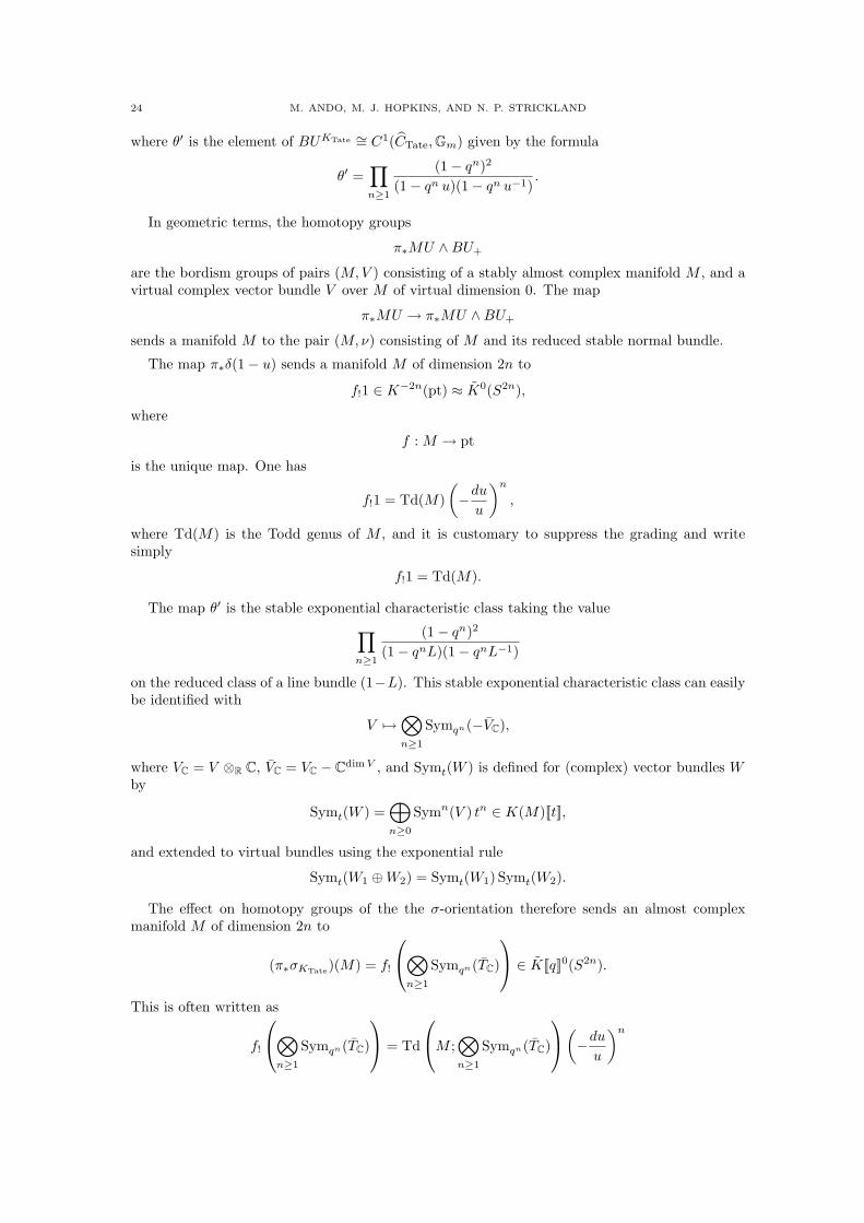
24 M. ANDO, M. J. HOPKINS, AND N. P. STRICKLAND
where θ′ is the element of BUKTate ∼= C1(CTate,Gm) given by the formula
θ′ =∏
n≥1
(1− qn)2
(1− qn u)(1− qn u−1).
In geometric terms, the homotopy groups
π∗MU ∧BU+
are the bordism groups of pairs (M,V ) consisting of a stably almost complex manifold M , and avirtual complex vector bundle V over M of virtual dimension 0. The map
π∗MU → π∗MU ∧BU+
sends a manifold M to the pair (M,ν) consisting of M and its reduced stable normal bundle.
The map π∗δ(1− u) sends a manifold M of dimension 2n to
f!1 ∈ K−2n(pt) ≈ K0(S2n),
where
f : M → pt
is the unique map. One has
f!1 = Td(M)(−du
u
)n
,
where Td(M) is the Todd genus of M , and it is customary to suppress the grading and writesimply
f!1 = Td(M).
The map θ′ is the stable exponential characteristic class taking the value∏
n≥1
(1− qn)2
(1− qnL)(1− qnL−1)
on the reduced class of a line bundle (1−L). This stable exponential characteristic class can easilybe identified with
V 7→⊗
n≥1
Symqn(−VC),
where VC = V ⊗R C, VC = VC − Cdim V , and Symt(W ) is defined for (complex) vector bundles Wby
Symt(W ) =⊕
n≥0
Symn(V ) tn ∈ K(M)[[t]],
and extended to virtual bundles using the exponential rule
Symt(W1 ⊕W2) = Symt(W1) Symt(W2).
The effect on homotopy groups of the the σ-orientation therefore sends an almost complexmanifold M of dimension 2n to
(π∗σKTate)(M) = f!
⊗
n≥1
Symqn(TC)
∈ K[[q]]0(S2n).
This is often written as
f!
⊗
n≥1
Symqn(TC)
= Td
M ;
⊗
n≥1
Symqn(TC)
(−du
u
)n
ELLIPTIC SPECTRA 25
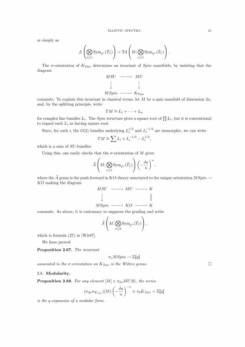
or simply as
f!
⊗
n≥1
Symqn(TC)
= Td
M ;
⊗
n≥1
Symqn(TC)
.
The σ-orientation of KTate determines an invariant of Spin–manifolds, by insisting that thediagram
MSU −−−−→ MUyy
MSpin −−−−→ KTate
commute. To explain this invariant in classical terms, let M be a spin manifold of dimension 2n,and, by the splitting principle, write
TM ∼= L1 + · · ·+ Ln
for complex line bundles Li. The Spin structure gives a square root of∏
Li, but it is conventionalto regard each Li as having square root.
Since, for each i, the O(2) bundles underlying L1/2i and L
−1/2i are isomorphic, we can write
TM ∼=∑
Li + L−1/2i − L
1/2i ,
which is a sum of SU -bundles.
Using this, one easily checks that the σ-orientation of M gives
A
M ;
⊗
n≥1
Symqn(TC)
(−du
u
)n
,
where the A genus is the push-forward in KO-theory associated to the unique orientation MSpin →KO making the diagram
MSU −−−−→ MU −−−−→ Ky
∥∥∥MSpin −−−−→ KO −−−−→ K
commute. As above, it is customary to suppress the grading and write
A
M ;
⊗
n≥0
Symqn(TC)
,
which is formula (27) in [Wit87].
We have proved
Proposition 2.67. The invariant
π∗MSpin → Z[[q]]
associated to the σ-orientation on KTate is the Witten genus.
2.8. Modularity.
Proposition 2.68. For any element [M ] ∈ π2nMU〈6〉, the series
(π2nσKTate)(M)(−du
u
)−n
∈ π0KTate = Z[[q]]
is the q-expansion of a modular form.
26 M. ANDO, M. J. HOPKINS, AND N. P. STRICKLAND
Proof. Let us write
Φ(M) = (π2nσKTate)(M)(−du
u
)−n
.
The discussion in the preceding section shows that Φ(M) defines holomorphic function on D, withintegral q-expansion coefficients. It suffices to show that, if π : H → D is the map
π(τ) = e2πiτ ,
then π∗Φ(M) transforms correctly under the action of SL2Z. This follows from the discussion ofHΛ in the introduction.
3. Calculation of Ck(Ga,Gm)
In this section, we calculate the structure of the schemes Ck(Ga,Gm) for 1 ≤ k ≤ 3, so as tobe able to compare them to BU〈2k〉HP in §4.
3.1. The cases k = 0 and k = 1. The group C0(Ga,Gm)(R) is just the group of invertibleformal power series f ∈ R[[x]]; and C1(Ga,Gm) is the group of formal power series f ∈ R[[x]] withf(0) = 1. Let R0 = Z[b0, b
−10 , b1, b2, . . . ], and let R1 = Z[b1, b2, b3, . . . ]. If Fk ∈ Ck(Ga,Gm)(Rk)
are the power series
F0 =∑
i≥0
bixi
F1 = 1 +∑
i≥1
bixi,
then the following is obvious.
Proposition 3.1. For k = 0 and k = 1, the ring Rk represents the functor Ck(Ga,Gm), withuniversal element Fk. v
Note that F0 has a unique product expansion
F0 = a0
∏
n≥1
(1− anxn) (3.2)
The ai give a different polynomial basis for R0 and R1.
3.2. The strategy for k = 2 and k = 3. For k ≥ 2, the group Ck(Ga,Gm)(R) is the group ofsymmetric formal power series f ∈ R[[x1, . . . , xk]] such that f(x1, . . . , xk−1, 0) = 1 and
f(x1, x2, . . . )f(x0 + x1, . . . )−1f(x0, x1 + x2, . . . )f(x0, x1, . . . )−1 = 1.
In the light of Remark 2.12, we can replace the normalization f(x1, . . . , xk−1, 0) = 1 by f(0, . . . , 0) =1. Alternatively, by symmetry, we can replace it by the condition that f(x1, . . . , xk) = 1(mod
∏j xj).
Similarly, the group Ck(Ga, Ga)(R) is the group of symmetric formal power series f ∈ R[[x1, . . . , xk]]such that f(x1, . . . , xk−1, 0) = 0 and
f(x1, x2, . . . )− f(x0 + x1, . . . ) + f(x0, x1 + x2, . . . )− f(x0, x1, . . . ) = 0.
We write Ckd(Ga, Ga)(R) for the subgroup consisting of polynomials of homogeneous degree d.
Our strategy for constructing the universal 2 and 3-cocycles is based on the following simpleobservation.
Lemma 3.3. Suppose that h ∈ Ck(Ga,Gm)(R), and that h = 1 mod (x1, . . . , xk)d. Then thereis a unique cocycle c ∈ Ck
d(Ga, Ga) such that h = 1 + c mod (x1, . . . , xk)d+1. If g and h aretwo elements of Ck(Ga,Gm) of the form 1 + c mod (x1, . . . , xk)d+1, then g/h is an element ofCk(Ga,Gm) of the form 1 mod (x1, . . . , xk)d+1.
ELLIPTIC SPECTRA 27
We call c the leading term of h. We first calculate a basis of homogeneous polynomials for thegroup of additive cocycles. Then we attempt construct multiplicative cocycles with study withour homogeneous additive cocycles as leading term. The universal multiplicative cocycle is theproduct of these multiplicative cocycles. Much of the work in the case k = 3 is showing howadditive cocycles can occur as leading multiplicative cocycles.
In the cases k = 0 and k = 1, this procedure leads to the product description (3.2) of invertiblepower series.
We shall use the notation
δ× : Ck−1(Ga,Gm) → Ck(Ga,Gm)
for the map given in Definition 2.20, and reserve δ for the map
δ : Ck−1(Ga, Ga) → Ck(Ga, Ga).
Definition 2.20 gives these maps for k ≥ 2; for f ∈ C0(Ga,Gm)(R) we define
δ×f(x1) = f(0)f(x1)−1
and similarly for C0(Ga, Ga).
3.3. The case k = 2. Although we shall see (Proposition 3.12) that the ring OC2(bGa,Gm) ispolynomial over Z, the universal 2-cocycle F2 does not have a product decomposition
F2 =∏
d≥2
g2(d, bd),
with g2(d, bd) having leading term of degree d, until one localizes at a prime p. The analogousresult for H∗BSU is due to Adams [Ada76].
Fix a prime p. For d ≥ 2, let c(d) ∈ Z[x1, x2] be the polynomial
c(d) =
1p (xd
1 + xd2 − (x1 + x2)d) d = ps for some s ≥ 1
xd1 + xd
2 − (x1 + x2) otherwise(3.4)
The following calculation of C2(Ga, Ga) is due to Lazard; it is known as the “symmetric 2-cocycle lemma”. A proof may be found in [Ada74].
Lemma 3.5. Let A be a Z(p)-algebra. For d ≥ 2, the group C2d(Ga, Ga)(A) is the free A-module
on the single generator c(d).
Let
E(t) = exp
∑
k≥0
tpk
pk
(3.6)
be the Artin-Hasse exponential (see for example [Haz78]). It is of the form 1 mod (t), and it hascoefficients in Z(p).
For d ≥ 2, let g2(d, b) ∈ C2(Ga,Gm)(Q[b]) be the power series
g2(d, b) =
δ2×(E(bxd)−p) if d is a power of p
δ2×(E(bxd)) otherwise.
(3.7)
Using the formulae for the polynomials c(d) and the Artin-Hasse exponential, it is not hard tocheck that g2(d, b) belongs to the ring Z(p)[b][[x1, x2]], and that it is of the form
g2(d, b) = 1 + bc(d) mod (x1, x2)d+1. (3.8)
We give the proof as Corollary 3.22.
28 M. ANDO, M. J. HOPKINS, AND N. P. STRICKLAND
Now let R2 be the ring
R2 = Z(p)[a2, a3, . . . ],
and F2 ∈ C2(Ga,Gm)(R2) be the the cocycle
F2 =∏
d≥2
g2(d, ad).
Proposition 3.9. The ring R2 represents C2(Ga,Gm)× spec(Z(p)), with universal element F2.
Proof. Let A be a Z(p)-algebra, and let h ∈ C2(Ga,Gm)(A) be a cocycle. By Lemma 3.5 and theequation (3.8), there is a unique element a2 ∈ A such that
h
g2(2, a2)= 1 mod (x1, x2)3
in C2(Ga,Gm)(A). Proceeding by induction yields a unique homomorphism from R2 to A, whichsends the cocycle F2 to h.
3.4. The case k = 3: statement of results. The analysis of C3(Ga,Gm) is more complicatedthan that of of C2(Ga,Gm) for two reasons. First, the structure of C3(Ga, Ga) is more compli-cated; in addition, it is a more delicate matter to prolong some of the additive cocycles c intomultiplicative ones of the form 1 + bc + . . . . This is reflected in the answer: although the ringrepresenting C2(Ga,Gm) is polynomial, the ring representing C3(Ga,Gm) × spec(Z(p)) containsdivided polynomial generators.
Definition 3.10. We write D[x] for the divided-power algebra on x over Z. It has a basis con-sisting of the elements x[m] for m ≥ 0; the product is given by the formula
x[m]x[n] =(m + n)!
m!n!x[m+n].
If R is a ring then we write DR[x] for the ring R⊗D[x].
We summarize some well-known facts about divided-power algebras in §3.4.1.
Fix a prime p. Let R3 be the ring
R3 = Z(p)[ad|d ≥ 3 not of the form 1 + pt]⊗⊗
t≥1
DZ(p) [a1+pt ].
In §3.6.1, we construct an element F3 ∈ C3(Ga,Gm). In Proposition 3.28, we show that the mapclassifying F3 gives an isomorphism
Z3 = spec R3 −→∼= C3(Ga,Gm)× spec(Z(p)). (3.11)
The plan of the rest of this section is as follows. In §3.5, we describe the scheme Ck(Ga, Ga).We calculate Ck(Ga, Ga)× specQ for all k, and we calculate C3(Ga, Ga)× specFp. The proofs ofthe main results are given in Appendix A.
In §3.6, we construct multiplicative cocycles with our additive cocycles as leading terms. Thiswill allow us to write a cocycle Z3 over R3 in §3.6.1. For some of our additive cocycles in charac-teristic p (precisely, those we call c′(d)), we are only able to write down a multiplicative cocycleof the form 1 + ac′(d) by assuming that ap = 0 (mod p); these correspond to the divided-powergenerators in R3.
In §3.7, we show that the condition ap = 0 (mod p) is universal, completing the proof of theisomorphism (3.11).
ELLIPTIC SPECTRA 29
3.4.1. Divided powers. For convenience we recall some facts about divided-power rings.
i. A divided power sequence in a ring R is a sequence
(1 = a[0], a = a[1], a[2], a[3], . . . )
such that
a[m]a[n] =(m + n)!
m!n!a[m+n]
for all m,n ≥ 0. It follows that am = m!a[m]. We write D1(R) for the set of divided powersequences in R. It is clear that D1 = spec D[x].
ii. An exponential series over R is a series α(x) ∈ R[[x]] such that α(0) = 1 and α(x + y) =α(x)α(y). We write Exp(R) for the set of such series. It is a functor from rings to abeliangroups.
iii. Given a ∈ D1(R), we define exp(a)(x) =∑
m≥0 a[m]xm ∈ R[[x]]. By a mild abuse, we allowourselves to write exp(ax) for this series. It is an exponential series, and the correspondencea 7→ exp(a)(x) gives an isomorphism of functors D1 ∼= Exp. In particular both are groupschemes.
iv. The map Q[x] → DQ[x] sending x to x has inverse x[m] 7→ xm/m!, and this gives an isomor-phism
D1 × spec(Q) ∼= A1 × spec(Q).
v. We write Tp[x] for the truncated polynomial ring Tp[x] = Fp[x]/xp, and we write αp =spec Tp[x]. Thus αp(R) is empty unless R is an Fp-algebra, and in that case αp(R) = a ∈R | ap = 0.
vi. Given a Z(p)-algebra R and an element a ∈ R, we define texp(ax) =∑p−1
k=0 akxk/k!. Here wecan divide by k! because it is coprime to p.
vii. Over Fp the divided power ring decomposes as a tensor product of truncated polynomial rings
DFp [x] ∼=⊗
r≥0
Tp[x[pr ]]
Moreover there is an equation
exp(ax) =∏
r≥0
texp(a[pr ]xpr
) (mod p).
Each factor on the right is separately exponential: if a ∈ αp(R) then
texp(a(x + y)) = texp(ax) texp(ay).
In other words, the map
a 7→ (a[1], a[p], a[p2], . . . )
gives an isomorphism
D1 × spec(Fp) =∏
m≥0
αp,
and the resulting isomorphism∏
m≥0
αp∼= Exp× spec(Fp)
is given by
b 7→∏
m≥0
texp(bmxpm
).
30 M. ANDO, M. J. HOPKINS, AND N. P. STRICKLAND
3.4.2. Grading. It will be important to know that the maps OCk(bGa,Gm) → Rk we construct maybe viewed as maps of connected graded rings of finite type: a graded ring R∗ is said to be of finitetype over Z if each Rn is a finitely generated abelian group.
We let Gm act on the scheme Ck(Ga,Gm) by
(u.h)(x1, . . . , xk) = h(ux1, . . . , uxk),
and give OCk(bGa,Gm) the grading associated to this action. One checks that the coefficient ofxα =
∏i xαi
i in the universal cocycle has degree |α| =∑
i αi. If k > 0 then the constant term is1 and the other coefficients have strictly positive degrees tending to infinity, so the homogeneouscomponents of OCk(bGa,Gm) have finite type over Z.
The divided power ring D[x] can be made into a graded ring by setting |x[m]| = m|x|. We canthen grade our rings Rk by setting the degree of ad to be d. It is clear that R1 is a connectedgraded ring of finite type over Z, and Rk is a connected graded ring of finite type over Z(p) fork > 1.
This can be described in terms of an action of Gm on Zk = spec Rk. We have
Z0∼= Gm ×
∏
d≥1
A1
Z1∼=
∏
d≥1
A1
Z2∼=
∏
d≥2
A1 × specZ(p)
Z3∼=
∏
d≥3
Z3,d
where
Z3,d =
A1 × specZ(p) d 6= 1 + pt
D1 × specZ(p) d = 1 + pt.
We let Gm act on A1 or Gm by u.a = ua, and on D1 by (u.a)[k] = uka[k]. We then let Gm act onZk by
u.(ak, ak+1, . . . ) = (uk.ak, uk+1.ak+1, . . . ).
The resulting grading on Rk is as described. For k ≤ 2, it is easy to check that the map Zk →Ck(Ga,Gm) classifying Fk is Gm-equivariant.
As an example of the utility of the gradings, we have the following.
Proposition 3.12. The ring OC2(bGa,Gm) is polynomial over Z on countably many homogeneousgenerators.
Proof. As OC2(bGa,Gm) is a connected graded ring of finite type over Z, it suffices by well-knownarguments to check that Z(p)⊗OC2(bGa,Gm) is polynomial on homogeneous generators for all primesp. By Proposition 3.9, we have an isomorphism of rings Z(p)⊗OC2(bGa,Gm)
∼= OZ2 = Z(p)[ad | d ≥ 2],and it is easy to check that ad is homogeneous of degree d.
3.5. Additive cocycles. In this section we describe the group Ck(Ga, Ga)(A) for various k andA. The results provide the list of candidates for leading terms of multiplicative cocycles. Proofsare given in the appendix A.
Fix an integer k ≥ 1. We write Ck(A) for Ck(Ga, Ga)(A), and we write Ckd (A) for the subgroup
Ckd(Ga, Ga) of series which are homogeneous of degree d. Note that Ck
d (A) = 0 for d < k.
ELLIPTIC SPECTRA 31
Given a set I ⊆ 1, . . . , k we write xI =∑
i∈I xi. One can easily check that for g ∈ A[[x]] =C0(A) we have
(δkg)(x1, . . . , xk) =∑
I
(−1)|I|g(xI).
For example, if g(x) = xd then
(δ2g)(x, y) = (x + y)d − xd − yd
(δ3g)(x, y, z) = −(x + y + z)d + (x + y)d + (x + z)d + (y + z)d − xd − yd − zd.
3.5.1. The rational case. Rationally, the cocycles δkxd for d ≥ k are a basis for the additivecocycles.
Proposition 3.13 (A.1). If A is a Q-algebra, then for d ≥ k the group Ckd (A) is the free abelian
group on the single generator δkxd.
3.5.2. Divisibility. Now we fix an integer k ≥ 2 and a prime p.
Definition 3.14. For all n let νp(n) denote the p-adic valuation of n. For d ≥ k we let u(d) bethe greatest common divisor of the coefficients of the polynomial δk(xd). We write v(d) for thep-adic valuation νp(u(d)). Let c(d) be the polynomial c(d) = ((−δ)k(xd))/pv(d) ∈ Z[x1, . . . , xk](We have put a sign in the definition to ensure that c(d) has positive coefficients). It is clear that
c(d) ∈ Ckd (Z).
If we wish to emphasize the dependence on k, we write uk(d), ck(d), and vk(d).
We will need to understand the integers v(d) more explicitly.
Definition 3.15. For any nonnegative integer d and any prime p, we write σp(d) for the sum ofthe digits in the base p expansion of d. In more detail, there is a unique sequence of integers di
with 0 ≤ di < p and∑
i dipi = d, and we write σp(d) =
∑i di.
The necessary information is given by the following result, which will be proved in Appendix A.
Proposition 3.16 (A.10). For any d ≥ k we have
v(d) = max(
0,
⌈k − σp(d)
p− 1
⌉).
The important examples of Proposition 3.16 for the present paper are k = 2 and k = 3:
Corollary 3.17.
v2(d) =
1 σp(d) = 10 otherwise
v3(d) =
2 σ2(d) = 1 and p = 21 σp(d) = 1 and p > 21 σp(d) = 20 σp(d) > 2.
In other words, v2(d) = 1 if d is a power of p, and 0 otherwise. We have v3(d) = 2 if p = 2 andd has the form 2t with t > 1, and v3(d) = 1 if p = 2 and d has the form 2s(1 + 2t). On the otherhand, when p > 2 we have v3(d) = 1 if d has the form pt or 2pt or ps(1 + pt) (with s ≥ 0 andt > 0). In all other cases we have v3(d) = 0.
In particular, the calculation of v2(d) shows that the cocycle c2(d) in Definition 3.14 coincideswith the cocycle c(d) in the formula (3.4).
32 M. ANDO, M. J. HOPKINS, AND N. P. STRICKLAND
3.5.3. The modular case. We continue to fix an integer k ≥ 2 and a prime p, and we analyzeCk(A) when p = 0 in A.
For any ring A we define an endomorphism φ of A[[x1, . . . , xk]] by φ(xi) = xpi . If p = 0 in A one
checks that this sends Ck(A) to Ck(A) and Ckd (A) to Ck
dp(A). Moreover, if A = Fp then ap = a
for all a ∈ Fp and thus φ(h) = hp.
In particular, we can consider the element φjc(d) ∈ Z[x1, . . . , xk], whose reduction mod p liesin Ck
pjd(Fp). The following proposition shows that this rarely gives anything new.
Proposition 3.18. If νp(d) ≥ v(d) then
c(pjd) = c(d)pj
= φjc(d) (mod pνp(d)−v(d)+1).
It is clear from Proposition 3.16 that v(pd) = v(d), so even if the above proposition does notapply to d, it does apply to pid for large i.
Proof. We can reduce easily to the case j = 1. Write v = v(pd) = v(d), so that c(d) =(−δ)k(xd)/pv and c(pd) = (−δ)k(xpd)/pv. Write w = vp(d), so the claim is equivalent to theassertion that
φ(−δ)k(xd) = (−δ)k(xpd) (mod pw+1).
The left hand side is∑
I ±φ(xdI) =
∑I ±φ(xI)d. It is well-known that φ(xI) = (xI)p (mod p), and
that whenever we have a = b (mod p) we also have api
= bpi
(mod pi+1). It follows easily thatφ(xI)d = (xI)pd (mod pw+1). As the right hand side of the displayed equation is just
∑I ±(xI)pd,
the claim follows.
3.5.4. The case k = 3. In this section we set k = 3, and we give basis for the group of additivethree-cocycles over an Fp-algebra. In order to describe the combinatorics of the situation, it willbe convenient to use the following terminology.
Definition 3.19. We say that an integer d ≥ 3 has type
I if d is of the form 1 + pt with t > 0.II if d is of the form ps(1 + pt) with s, t > 0.
III otherwise.
If d = ps(1 + pt) has type I or II we define c′(d) = φsc(1 + pt) ∈ C3d(Fp). Note that d has type I
precisely when σp(d− 1) = 1, and in that case we have c′(d) = c(d).
Proposition 3.20 (A.12). If A is an Fp-algebra then C3(A) is a free module over A generatedby the elements c(d) for d ≥ 3 and the elements c′(d) for d of type II.
3.6. Multiplicative cocycles. We fix a prime p and an integer k ≥ 1. In this section we writedown the basic multiplicative cocycles. We need the following integrality lemma; many similarresults are known (such as [Haz78, Lemma 2.3.3]) and this one may well also be in the literaturebut we have not found it.
Lemma 3.21. Let A be a torsion-free p-local ring, and φ : A −→ A a ring map such that φ(a) = ap
(mod p) for all a ∈ A. If (bk)k>0 is a sequence of elements such that φ(bk) = bk+1 (mod pk+1)for all k, then the series exp(
∑k bkxpk
/pk) ∈ (Q⊗A)[[x]] actually lies in A[[x]].
Proof. Write f(x) = exp(∑
k bkxpk
/pk). Clearly f(0) = 1, so there are unique elements aj ∈ Q⊗Asuch that f(x) =
∏j>0 E(ajx
j), and it is enough to show that aj ∈ A for all j. By taking logs wefind that
∑
k
bkxpk
/pk =∑
i,j
api
j xjpi
/pi.
ELLIPTIC SPECTRA 33
It follows that aj = 0 unless j is a power of p, and that bk =∑
k=i+j piapj
pi . We may assumeinductively that a1, ap, . . . , apj−1 are integral. It follows that for i < j we have φ(api) = ap
pi
(mod p), and thus (by a well-known lemma) that
φ(apj−i−1
pi ) = φ(api)pj−i−1= apj−i
pi (mod pj−i).
It follows that
pjapj = bj −j−1∑
i=0
piapj−i
pi
= bj −j−1∑
i=0
piφ(api)pj−i−1(mod pj)
= bj − φ(bj−1)
= 0 (mod pj),
or in other words that apj is integral.
Recall from (3.6) that E(t) ∈ Z(p)[[t]] denotes the Artin-Hasse exponential.
Corollary 3.22. If d is such that νp(d) ≥ v(d), then δk×E(bxd)p−v(d) ∈ Q[b][[x1, . . . , xk]] actually
lies in Ck(Ga,Gm)(Z(p)[b]) ⊆ Z(p)[b][[x1, . . . , xk]]. It has leading term bc(d).
Proof. The symmetric cocycle conditions are clear, so we need only check that the series is integral.Using the exp in the Artin-Hasse exponential gives the formula
δk×E(bxd)p−v(d)
= exp
∑
i≥0
bpi
δk(xdpi
)pi+v(d)
= exp
∑
i≥0
bpi
c(dpi)pi
.
In view of Lemma 3.21, it suffices to check that φ(c(dpi)) = c(dpi+1) (mod pi+1), where φ is theendomorphism of Z(p)[[x1, . . . , xk]] given by φ(xi) = xp
i . This follows from Proposition 3.18.
Definition 3.23. If R is a Z(p)-algebra, b is an element of R, and if d is such that νp(d) ≥ v(d),we define
E(k, d, b) def= δk×E(bxd)p−v(d)
to be the element of Ck(Ga,Gm)(R) given by the corollary.
In order to analyze the map δ×, we need the following calculation.
Lemma 3.24. If νp(d) ≥ v(d) we have
E(k, d, b)p = E(k, pd, bp) (mod p).
Proof. We can work in the universal case, where A = Z(p)[b] is torsion-free, so it makes sense touse exponentials. We have
E(k, d, b) = exp(∑
k
bpk
c(pkd)/pk),
and it follows easily that E(k, d, b)p/E(k, pd, ap) = exp(pac(d)). One checks easily that the seriesexp(pt)− 1 has coefficients in pZ(p), and the claim follows.
We need one other family of cocycles, given by the following result.
Proposition 3.25. Let B be the divided-power algebra on one generator b over Z(p). Then theseries δk
× exp(bxd/pv(d)) = exp((−1)kb c(d)) lies in Ck(Ga,Gm)(B) ⊆ B[[x1, . . . , xk]].
34 M. ANDO, M. J. HOPKINS, AND N. P. STRICKLAND
3.6.1. The case k = 3. Suppose that d ≥ 3 is not of the form 1 + pt. Then Corollary 3.17 showsthat νp(d) ≥ v(d), and so Definition 3.23 gives cocycles
g3(d, ad)def= E(3, d, ad) ∈ C3(Ga,Gm)(Z(p)[ad]). (3.26)
For d = 1 + pt and t ≥ 1, let
g3(d, ad)def= exp(−ad c(d)) ∈ C3(Ga,Gm)(DZ(p) [ad])
be the cocycle given by Proposition 3.25.
Note that if d = 1 + pt then in Fp ⊗DZ(p) [ad] we have an equation
g3(d, ad) =∏
s≥0
texp(−a[ps]d c′(dps)) (3.27)
as in §3.4.1, and each factor on the right is separately an element of C3(Ga,Gm)(Tp[a[ps]d ]).
Let F3 be the cocycle
F3 =∏
d≥3
g3(d, ad)
over
Z3 = specZ(p)[ad | d 6= 1 + pt]⊗⊗
t≥1
DZ(p) [a1+pt ].
Proposition 3.28. The map Z3 → C3(Ga,Gm)× spec(Z(p)) classifying F3 is an isomorphism.
Proof. Let h denote this map. It is easy to check that it is compatible with the Gm-actionsdescribed in §3.4.2, so the induced map of rings preserves the gradings.
We will show that the map h(R) : Z3(R) −→ C3(Ga,Gm)(R) is an isomorphism when R is aQ-algebra or an Fp-algebra. This means that the map h∗ : OC3(bGa,Gm) ⊗ Z(p) −→ OZ3 becomes anisomorphism after tensoring with Q or Fp. As both sides are connected graded rings of finite typeover Z(p), it follows that h is itself an isomorphism.
Suppose that R is a Q-algebra. In this case we get divided powers for free, and an elementof Z3(R) is just a list of elements (a3, a4, . . . ). According to Proposition 3.13, the additive co-cycle c(d) generates C3
d(Ga, Ga)(R). Since gd has leading term adc(d), the process of successiveapproximation suggested by Lemma 3.3 shows that h(R) is an isomorphism.
We now suppose instead that R is an Fp-algebra. As DFp [x] = Tp[x[pi] | i ≥ 0], we see that a
point of Z3(R) is just a sequence of elements ad ∈ R for d ≥ 3, with additional elements ad,i = a[pi]d
when d has type I, such that ad,0 = ad and apd,i = 0. We write a′dpi = ad,i. With this reindexing,
an element of Z3(R) is a system of elements ad (where d has type II or III) together with a systemof elements a′d (where d has type I or II) subject only to the condition (a′d)
p = 0.
On the other hand, suppose that f ∈ C3(Ga,Gm)(R) is a cocycle with leading term c of degreed. If d has type III, then Proposition 3.20 shows that c = adc(d) for a unique c in R. If d has typeI, then c = a′d,0c
′(d) for some unique a′d,0 in R. Finally, if d has type II, then c = adc(d) + a′dc′(d)
for some unique ad and a′d in R. We shall show in Proposition 3.29 that in fact (a′d)p = 0. The
process of successive approximation gives a point of Z3(R) which clearly maps to f under the maph(R).
In the course of the proof, we used the following result, whose proof will be given in §3.7.
Proposition 3.29. Suppose that R is an Fp-algebra and that f ∈ C3(Ga,Gm)(R) has leadingterm ac′(d) (so that d has type I or II). Then ap = 0.
Corollary 3.30. The ring OC3(bGa,Gm) is a graded free abelian group of finite type.
ELLIPTIC SPECTRA 35
Proof. Proposition 3.28 shows that this is true p-locally for every prime p, so it is true integrally.
3.7. The Weil pairing: cokernel of δ× : C2(Ga,Gm) → C3(Ga,Gm). The first result of thissection is a proof of Proposition 3.29, which completes the calculation in Proposition 3.28. Theanalysis which leads to this result also gives a description of the cokernel of the map
C2(Ga,Gm)δ×−→ C3(Ga,Gm),
which we shall use to compare C3(Ga,Gm) to BU〈6〉HP .
More precisely, the scheme Z3 decomposes as a product of schemes
Z3 = Z ′3 × Z′′3where
Z ′3 = spec DZ(p) [a1+pt | t ≥ 1]
Z ′′3 = specZ(p)[ad | d not of the form 1 + pt].
We shall show that δ× maps C2(Ga,Gm) × specFp surjectively onto Z ′′3 × specFp, and that thecokernel Z′3 × specFp has a natural description as the scheme Weil(Ga) of Weil pairings. In§4.5.1, we shall see that this scheme is isomorphic to the scheme associated to the even homol-ogy of K(Z, 3). In this paper we give a bare-bones account of Weil pairings. The reader canconsult [Bre83, Mum65, AS98] for a more complete treatment.
Definition 3.31. Let R be any ring, and h an element of C3(Ga,Gm)(R). We define a seriese(h) ∈ R[[x, y]] by the formula
e(h)(x, y) =p−1∏
k=1
h(x, kx, y)h(x, ky, y)
.
In §3.7.1, e will be interpreted as giving a map of group schemes
C3(Ga,Gm)× specFp −→ Weil(Ga).
Proposition 3.32. We have
e(h)(x, y) e(h)(x, z) = e(h)(x, y + z)h(px, y, z)h(x, py, pz)
= e(h)(x, y + z) (mod p),
and e(h)(x, y)p = 1 (mod p).
Proof. Recall the cocycle relation R(w, x, y, z) = 1, where
R(w, x, y, z) =h(x, y, z)h(w, x + y, z)h(w + x, y, z)h(w, x, z)
.
By brutally expanding the relation
R(y, z, k(y + z), x)R(ky, (k + 1)z, y, x)R((k + 1)z, y, ky, x)
R(ky, kz, z, x)R(kx, x, y, z)R(x, y, z, kx) = 1,
and using the symmetry of h, we find thath(x, kx, y)h(x, ky, y)
.h(x, kx, z)h(x, kz, z)
=h(x, kx, y + z)
h(x, ky + kz, y + z).
h(x, ky, kz)h(x, (k + 1)y, (k + 1)z)
.h((k + 1)x, y, z)
h(kx, y, z)We now take the product from k = 1 to p− 1. We note that the second term on the right has theform f(k)/f(k + 1), so the product gives f(1)/f(p). After dealing with the last term in a similarway and doing some cancellation, we find that
e(h)(x, y) e(h)(x, z) = e(h)(x, y + z) h(px, y, z)h(x, py, pz)−1,
36 M. ANDO, M. J. HOPKINS, AND N. P. STRICKLAND
as claimed. For any cocycle h we have h = 1 (mod xyz), so our expression reduces to e(h)(x, y+z)modulo p. This means that e(h) behaves exponentially in the second argument, so e(h)(x, y)p =e(h)(x, py) = 1 (mod p).
We can also consider an additive analogue of the above construction. Given c ∈ C3(Ga, Ga)(R),we write
e+(c)(x, y) =p−1∑
k=1
(c(x, kx, y)− c(x, ky, y)).
By applying the definitions and canceling in a simple-minded manner we find that
e+(δ3f)(x, y) = f(x)− f(x + py)− f(y) + f(y + px)− f(px) + f(py).
Thus e+(δ3f) = 0 (mod p).
The following calculation is the key to the proof of Proposition 3.29, and it also permits theidentification of Z′3 with the scheme of Weil pairings.
Lemma 3.33. Let d = ps(1 + pt) with s ≥ 0 and t ≥ 1. Then
e+(c′(d)) = xps
yps+t − xps+t
yps
(mod p).
Proof. As c′(ps(1 + pt))p = c(1 + pt)ps+1, it suffices to calculate e+(c(1 + pt)) (mod p). Let
n = 1 + pt. By Corollary 3.17, we have c(n) = δ3(xn)/p, so that
pe+(c(n)) = xn − (x + py)n − yn + (y + px)n − pnxn + pnyn
= −pnxn−1y + pnxyn−1 (mod p2)
= p(xypt − xpt
y) (mod p2).
Thus e+(c(1 + pt)) = xypt − yxpt
(mod p) as required.
We can now give the
Proof of Proposition 3.29. Suppose that R is an Fp-algebra and that h ∈ C3(Ga,Gm)(R) hasleading term ac′(d) (so that d has type I or II).
It is easy to see that e(h) = 1 + ae+(c′(d)) (mod (x, y, z)d+1), and thus that e(h)p = 1 +ape+(c′(d))p (mod (x, y, z)pd+1). On the other hand, we know from Proposition 3.32 that e(h)p =1. Lemma 3.33 shows that e+(c′(d))p is a nonzero polynomial over Fp which is homogeneous ofdegree pd. It follows that ap = 0.
3.7.1. The scheme of Weil pairings. In this section we work implicitly over spec(Fp). We notethat a faithfully flat map of schemes is an epimorphism.
We also recall [DG70, III,§3,n. 7] that the category of affine commutative group schemes overFp is an abelian category, in which spec f : spec A → spec B is an epimorphism if and only iff : B → A is injective.
Let R be an Fp-algebra. We write Weil(Ga)(R) for the group (under multiplication) of formalpower series f(x, y) ∈ R[[x, y]] such that
f(x, x) = 1
f(x, y)f(x, z) = f(x, y + z)
f(x, z)f(y, z) = f(x + y, z).(3.34)
Note that this implies f(x, y)f(y, x) = 1 by a polarization argument. We write Weil(Ga)(R) = ∅if R is not an Fp-algebra.
ELLIPTIC SPECTRA 37
Proposition 3.32 shows that, if R is an Fp-algebra and h ∈ C3(Ga,Gm) is a three-cocycle, thene(h) is a Weil pairing. In other words, e may be viewed as a natural transformation
e : C3(Ga,Gm) −→ Weil(Ga).
In this section, we show that there is a commutative diagram
C2(Ga,Gm)δ×
//
²²²²
C3(Ga,Gm)e // // Weil(Ga)
Z ′′3 // // Z ′3 × Z ′′3
∼=OO
// // Z ′3
∼=OO
(3.35)
of group schemes over specFp, with exact rows and with epi, mono, and isomorphisms as indicated.In §4.5, we compare the top row to a sequence arising from the fibration K(Z, 3) → BU〈6〉 → BSU .
To begin, we note that Weil(Ga) is an affine group scheme over Fp. The representing ringOWeil(bGa) is the quotient of the ring Fp[akl | k, l ≥ 0] by the ideal generated by the coefficients of
the series f(x, x) − 1 and f(x + y, z) − f(x, z)f(y, z) and f(x, y + z) − f(x, y)f(x, z), where f isthe power series
f(x, y) =∑
aklxkyl.
We let Gm act on Weil(Ga) by (u.f)(x, y) = f(ux, uy), and this gives a grading on OWeil(bGa)
making it into a graded connected Hopf algebra over Fp. If
f(x, y) =∑
i,j
aijxiyj
is the universal Weil pairing, then the degree of aij is i + j.
Lemma 3.36. The ring OWeil(bGa) is a tensor product of rings of the form Fp[a]/ap. If f =∑aijx
iyj is the universal Weil pairing, then elements of the form apm,pn with m < n are a basisfor Ind(OWeil(bGa)).
Proof. Let us temporarily write A for OWeil(bGa). Note that if f(x, y) ∈ Weil(Ga)(R) we havef(x, y)p = f(x, py) = f(x, 0) = 1, and it follows that the Frobenius map for A is trivial. It followsfrom the structure theory of connected graded Hopf algebras over Fp that A is a tensor productof rings of the form Fp[a]/ap.
The dual of the group of indecomposables in A is easily identified with the kernel of the map
Weil(Ga)(Fp[ε]/ε2) −→ Weil(Ga)(Fp)
that is induced by the augmentation map Fp[ε]/ε2 −→ Fp. This kernel is the set of power series ofthe form 1+εg(x, y) (with g ∈ Fp[[x, y]]) such that 1+εg(x, x) = 0 and (1+εg(x, y))(1+εg(x, z)) =1 + εg(x, y + z) and (1 + εg(x, z))(1 + εg(y, z)) = 1 + εg(x + y, z). This reduces to the requirementthat g(x, y) be additive in both arguments, with g(x, x) = 0. The additivity means that g(x, y)must have the form
∑m,n bmnxpm
ypn
. Because g(x, x) = 0 we must have bmm = 0 (even if p = 2)and bmn = −bnm if m > n.
Let j denote the splitting map
Z ′3 → C3(Ga,Gm).
Note that Z ′3 is a group scheme, because
Z ′3 ∼=∏D1 × spec(Z(p)) ∼=
∏Exp× spec(Z(p)).
It is easy to check that j is a map of group schemes (even over spec(Z(p))). The first step in theanalysis of the diagram 3.35 is the following.
38 M. ANDO, M. J. HOPKINS, AND N. P. STRICKLAND
Proposition 3.37. The map of group schemes
ej : Z ′3 −→ Weil(Ga)
is an isomorphism.
Proof. First, when R is an Fp-algebra we can identify Z ′3(R) with∏
da ∈ R | ap = 0, where druns over integers d ≥ 3 of type I or II, and according to (3.27), j(a) is the cocycle
j(a) =∏
d
texp(−adc′(d)).
Lemma 3.33 shows that if d = ps(1 + pt) then
e(texp(−adc′(d)) = 1− ad(xps
yps+t − xps+t
yps
) (mod (x, y)d+1).
It follows that ej induces an isomorphism of indecomposables. Moreover, ej induces a map ofgraded rings ifOZ′3 is given the grading with a′d in dimension d. We thus a map of connected gradedalgebras, both of which are tensor products of polynomial algebras truncated at height p, and ourmap gives an isomorphism on indecomposables. It follows that the map is an isomorphism.
To show that Z ′′3 is the kernel of e, we first observe that C2(Ga,Gm) maps to the kernel.
Lemma 3.38. If R is an Fp-algebra and g ∈ C2(Ga,Gm)(R) then e(δ×g) = 1.
Proof. By definition we have δ×g(x, kx, y) = g(x, y)g(kx, y)/g((k + 1)x, y). As δ×g is symmetric,we have δ×g(x, ky, y) = g(x, y)g(x, ky)/g(x, (k + 1)y). By substituting these equations into thedefinition of e(δ×g) and canceling, we obtain e(δ×g)(x, y) = g(x, py)/g(px, y), which is 1 becausep = 0 in R.
Next we show that δ× actually factors through the inclusion Z ′′3 → C3(Ga,Gm). Let w and θbe given by the formulae
w(2) = 1
w(d) = v3(d)− v2(d) d ≥ 3
θ(d) = pw(d)d.
By Corollary 3.17, it is equivalent to set w(d) = 1 if d is of the form ps(1 + pr) with r ≥ 0,and w(d) = 0 otherwise. It follows also that θ gives a bijection from d | d ≥ 2 to d | d ≥3 and d is not of the form 1 + pt.
Let r : Z2 = spec R2 → Z ′′3 be given by the formula
r∗aθ(d) = apw(d)
d .
It is clear that r is faithfully flat.
Lemma 3.39. The diagram
C2(Ga,Gm)δ×−−−−→ C3(Ga,Gm)
∼=x
xZ2
r−−−−→ Z ′′3commutes over spec(Fp). In particular, over spec(Fp), δ× factors through a faithfully flat mapC2(Ga,Gm) → Z ′′3 .
Proof. This follows from the equations
δ×g2(d, a) = δ3×E(axd)p−v2(()d)
= E(3, d, a)pw(d)= E(3, θ(d), apw(d)
) = g3(θ(d), apw(d)).
ELLIPTIC SPECTRA 39
The only equation which is not a tautology is the third, which is Lemma 3.24. Actually the lemmadoes not apply in the case d = 2, but the result is valid anyway. One can see this directly fromthe definitions, using the fact that δ3(x2) = 0.
Proposition 3.40. The kernel of the map
e : C3(Ga,Gm) −→ Weil(Ga)
is Z ′′3 (which is thus a subgroup scheme). Moreover, we have C3(Ga,Gm) = Z ′3 × Z ′′3 as groupschemes.
Proof. We know from Lemma 3.38 that eδ× = 1, and faithfully flat maps are epimorphismsof schemes, so Lemma 3.39 implies that Z ′′ ≤ ker(e). As the map (f ′, f ′′) 7→ f ′f ′′ gives anisomorphism Z ′×Z ′′ −→ C3, and e : Z ′ −→ Weil(Ga) is an isomorphism, it follows that Z ′′ = ker(e).This means that Z ′′ is a subgroup scheme, and we have already observed before Proposition 3.37that the same is true of Z ′. It follows that C3 = Z ′ × Z ′′ as group schemes.
We summarize the discussion in this section as the following.
Corollary 3.41. If we work over spec(Fp) then the following sequence of group schemes is exact:
C2(Ga,Gm) δ−→ C3(Ga,Gm) e−→ Weil(Ga) → 0.
3.8. The map δ× : C1(Ga,Gm) → C2(Ga,Gm). In the course of comparing BSUHP to C2(Ga,Gm)in §4, we shall use the following analogue of Corollary 3.41.
Proposition 3.42. For each prime p, the map
C1(Ga,Gm)× spec(Fp)δ×−→ C2(Ga,Gm)× spec(Fp)
is faithfully flat.
Proof. In order to calculate δ×, it is useful to use the model for C1 which is analogous to ourmodel Z2 for C2. Let Z1 be the scheme
Z1 = specZ(p)[ad | d ≥ 1],
and let
F1def=
∏
d≥1
E(1, d, ad)
=∏
d≥1
E(adxd)
be the resulting cocycle over OZ1 . It is clear that the map
Z1 → C1(Ga,Gm)× spec(Z(p))
classifying F1 is an isomorphism. Thus if k = 1 or 2, and if R is a Z(p)-algebra, then Zk(R) is theset of sequences (ak, ak+1, . . . ) of elements of R.
For d ≥ 1 let θ(d) = pv2(d)d, with the convention that v2(1) = 1. The calculation of v2(d) inCorollary 3.17 shows that θ induces a bijection from the set d | d ≥ 1 to the set d | d ≥ 2. Letr : Z1 → Z2 be the map which sends a sequence a = (a1, a2, . . . ) ∈ Z1(R) to the sequence
r(a)θ(d) = apv2(d)
d .
Thus r is a product of copies of the identity map A1 → A1 (indexed by d | v(d) = 0), togetherwith some copies of the Frobenius map A1 → A1 (indexed by d | v(d) = 1). These maps are
40 M. ANDO, M. J. HOPKINS, AND N. P. STRICKLAND
faithfully flat, and so r is faithfully flat. The Proposition then follows once we know that thediagram
C1(Ga,Gm)× spec(Fp)δ×−−−−→ C2(Ga,Gm)× spec(Fp)
∼=x
x∼=Z1 × spec(Fp)
r−−−−→ Z2 × spec(Fp)
commutes. The commutativity of the diagram follows from the equations (modulo p)
δ×E(axd) = E(2, d, a)pv2(d)
= E(2, θ(d), apv2(d))
= g2(θ(d), apv2(d)).
The first and last equations are tautologies; the middle equation follows from Lemma 3.24.
3.9. Rational multiplicative cocycles. Given k > 0, let Yk(R) be the set of formal powerseries f(x) ∈ R[[x]] such that f(x) = 1 (mod xk). This clearly defines a closed subscheme Yk ⊂C0(Ga,Gm)
Proposition 3.43. Over spec(Q), the map δk× : Yk −→ Ck(Ga,Gm) is an isomorphism.
Proof. Let R be a Q-algebra, and let g ∈ R[[x1, . . . , xk]] be an element of Ck(Ga,Gm)(R). Weneed to show that g = δk
×(f) for a unique element f ∈ Yk(R). If I = (x1, . . . , xk) then g = 1(mod I) so the series log(g) = −∑
m>0(1 − g)m/m is I-adically convergent. One checks that itdefines an element of Ck(Ga,Ga)(R), so Proposition 3.13 tells us that there is a unique h ∈ R[[x]]with h = 0 (mod xk) and δk(h) = log(g). The series exp(h) =
∑m hm/m! is x-adically convergent
to an element of Yk(R), which is easily seen to be the required f .
4. Topological calculations
In this section we will compare our algebraic calculations with known topological calculations ofE∗BU , H∗BSU , and H∗BU〈6〉, and we deduce that BU〈k〉E = Ck(PE ,Gm) for k ≤ 3. We startwith the cases k = 0 and k = 1, which are merely translations of very well-known results. We thenprove the result for all k when E = HPQ (the rational periodic Eilenberg-MacLane spectrum);this is an easy calculation.
Next, we prove the case k = 2 with E = HP . It suffices to do this with coefficients in thefield Fp, and then it is easy to compare our analysis of the scheme C2(Ga,Gm) to the short exactsequence
PHP −→ BUHP −→ BSUHP .
For BU〈6〉 we recall Singer’s calculation of H∗(BU〈6〉;Fp), which is based on the fibration
K(Z, 3) −→ BU〈6〉 −→ BSU.
Most of the work in this section is to produce the topological analogue of the exact sequence
C2(Ga,Gm)δ×
// C3(Ga,Gm)e // Weil(Ga) // 0
of Corollary 3.41; see (4.9). Having done so, we can easily prove the isomorphism BU〈6〉E ∼=C3(PE ,Gm) for E = HPFp. The isomorphism for integral homology follows from the casesE = HPQ and E = HPFp. Using a collapsing Atiyah-Hirzebruch spectral sequence and itsalgebraic analogue, we deduce the case E = MP , and we find that MP0BU〈6〉 is free over MP0.It is then easy to deduce the isomorphism for arbitrary E.
ELLIPTIC SPECTRA 41
4.1. Ordinary cohomology. We begin with a brief recollection of the ordinary cohomology ofBU , in order to fix notation.
It is well-known that H∗BU is a formal power series algebra generated by the Chern classes.It follows easily that the corresponding thing is true for HP 0BU : we can define Chern classesck ∈ HP 0BU for k > 0 and we find that HP 0BU = Z[[ck | k > 0]]. We also put c0 = 1. Wedefine a series c(t) ∈ HP 0[[t]] by c(t) =
∑k≥0 cktk. We then define elements qk by the equation
tc′(t)/c(t) =∑
k qktk. The group of primitives is
Prim HP 0BU = ∑
i
niqi | ni ∈ Z ∼=∏
i>0
Z.
There is an inclusion S1 = U(1)j−→ U and a determinant map U
det−−→ S1 with det j = 1. These
give maps PBj−−→ BU
B det−−−→ P with B det Bj = 1, and the fiber of B det is BU〈4〉 = BSU . Infact, if i : BSU −→ BU is the inclusion then one sees easily that i + j : BSU × P −→ BU inducesan isomorphism of homotopy groups, so it is an equivalence.
We have HP 0P = Z[[x]] with B det∗ x = c1 and Bj∗c1 = x and Bj∗ck = 0 for k > 1. Itfollows (as is well-known) that the inclusion BSU −→ BU gives an isomorphism HP 0BSU =HP 0BU/c1 = Z[[ck | k > 1]].
In particular, both BU and BSU are even spaces.
The Hopf algebra HP0BU is again a polynomial algebra, with generators bk for k > 0. We alsoput b0 = 1. The pairing between this ring and HP 0BU satisfies
〈ck,∏
i
bαii 〉 =
1 if
∏i bαi
i = bk1
0 otherwise.
The group of primitives in HP0BU is generated by elements rk, which are characterized by theequation
t d log(b(t))/dt = t b′(t)/b(t) =∑
k
rktk.
4.2. The isomorphism for BU〈0〉 and BU〈2〉.Proposition 4.1. For k = 0 and k = 1 and for any even periodic ring spectrum E, the naturalmap
BU〈2k〉E −→ Ck(PE ,Gm)
is an isomorphism.
Proof. We treat the case k = 1, leaving the case k = 0 for the reader. A coordinate x on PE givesisomorphisms
OPE = E0P ∼= E0[[x]]
O∨PE= E0P ∼= E0β1, β2, . . .
E0(BU) ∼= E0[b1, b2, . . . ]
OC1(PE ,Gm)∼= E0[b′1, b
′2, . . . ].
Here the βi ∈ E0P are defined so 〈xi, βj〉 = δij , and bi = (E0ρ1)(βi), where ρ1 : P −→ BU classifiesthe virtual bundle 1 − L. The b′i are defined by writing the universal element of C1(PE ,Gm) as1 +
∑i≥1 b′ix
i.
By Definition 2.27, the map BUE → C1(PE ,Gm) classifies the element b ∈ E0BU⊗E0P ∼=E0BU [[x]] which is the adjoint of the map E0ρ1. It is easy to see that b =
∑i bix
i.
42 M. ANDO, M. J. HOPKINS, AND N. P. STRICKLAND
Recall that Cartier duality (2.2) gives an isomorphism
PE ∼= Hom(PE ,Gm).
The construction f 7→ 1/f gives a map
Hom(PE ,Gm) i−→ C1(PE ,Gm).
Corollary 4.2. The diagram
PE(B det)E
//
∼=²²
BUE
∼=²²
Hom(PE ,Gm) i // C1(PE ,Gm)
commutes.
Proof. It will be enough to show that the dual diagram of rings commutes. As E0BU is generatedover E0 by (E0ρ1)(E0P ), it suffices to check commutativity after composing with E0ρ1. It is thenclear, because B det ρ1 classifies det(1− L) ∼= L−1, and so has degree −1.
4.3. The isomorphism for rational homology and all k.
Proposition 4.3. For any k > 0 we have
HP 0(BU〈2k〉;Q) = HP 0(BU ;Q)/(c1, . . . , ck−1) = Q[[cn | n ≥ k]].
We also have an isomorphism
BU〈2k〉HPQ ∼= Ck(Ga,Gm)× spec(Q).
Proof. We have fibrations BU〈2k + 2〉 −→ BU〈2k〉 −→ K(Z, 2k). It is well-known that
H∗(K(Z, 2k);Q) = Q[u2k]
with |u2k| = 2k. We know that the map BU〈2k〉 −→ K(Z, 2k) induces an isomorphism on π2k(−)and we may assume inductively that H∗(BU〈2k〉;Q) = Q[[cn | n ≥ k]], so the Hurewicz theoremtells us that u2k hits a nontrivial multiple of ck. It now follows from the Serre spectral sequencethat
H∗(BU〈2k + 2〉;Q) = Q[[cn | n ≥ k + 1]] = H∗(BU ;Q)/(c1, . . . , ck).
Dually, we know that H∗(BU ;Q) is generated by primitive elements ri such that ri is dual to ci,and we find that H∗(BU〈2k〉;Q) = Q[ri | i ≥ k]. These are precisely the functions on C1(Ga,Gm)that are unchanged when we replace f ∈ C1(Ga,Gm)(R) by f exp(g) for some polynomial g ofdegree less than k, as we see from the definition of the ri. We see from the proof of Proposition 3.43that these are the same as the functions that depend only on δk−1
× (f), and thus that BU〈2k〉HPQ
can be identified with Ck(Ga,Gm)× spec(Q), as claimed.
4.4. The ordinary homology of BSU .
Proposition 4.4. The natural map
BSUHP −→ C2(Ga,Gm)
is an isomorphism.
ELLIPTIC SPECTRA 43
Proof. It is enough to prove this modulo p for all primes p, so fix one. Consider the diagram ofaffine commutative group schemes (in which everything is taken implicitly over Fp)
PHP //
∼=²²
BUHP //
∼=²²
BSUHP
²²
Hom(Ga,Gm) // C1(Ga,Gm)δ×
// C2(Ga,Gm).
The diagram commutes by Corollaries 2.28 and 4.2. The splitting BU = BSU × P implies thatthe top row is a short exact sequence. It is clear that Hom(Ga,Gm) is the kernel of δ×, so itremains to show that δ× is an epimorphism. That is precisely the content of Proposition 3.42.
4.5. The ordinary homology of BU〈6〉. The mod p cohomology of BU〈2k〉 was computed (forall k ≥ 0) by Singer [Sin68]. We next recall the calculation for k = 3. Note that BU〈6〉 is thefiber of a map BSU −→ K(Z, 4) and ΩK(Z, 4) = K(Z, 3) so we have a fibration
K(Z, 3)γ−→ BU〈6〉 v−→ BSU.
In this section we give an algebraic model for the ordinary homology of this fibration, in terms ofthe theory of symmetric cocycles and Weil pairings.
Classical calculations show that for p > 2 we have
H∗(K(Z, 3);Fp) = E[u0, u1, . . . ]⊗ Fp[βu1, βu2, . . . ],
where |uk| = 2pk +1 and uk+1 = P pk
uk and βu0 = 0. We write A∗ for the polynomial subalgebragenerated by the elements βuk for k > 0. We also write A =
∏k≥0 A2k, which is an ungraded
formal power series algebra over Fp. In the case p = 2 we have
H∗(K(Z, 3);F2) = F2[u0, u1, . . . ],
with |uk| = 2k+1 + 1 and uk+1 = Sq2k+1uk, and we let A∗ be the subalgebra generated by the
elements u2k. We write A∨∗ for the vector space dual Hom(A∗,Fp).
Lemma 4.5. In the Serre spectral sequence
H∗(BSU ; H∗(K(Z, 3);Fp)) =⇒ H∗(BU〈6〉;Fp)
the class ut survives to E2pt+2, and then there is a differential d2pt+2(ut) = q1+pt , up to a unit inFp.
Proof. We treat the case p > 2 and leave the (small) modifications for p = 2 to the reader. AsBU〈6〉 is 5-connected, we must have a transgressive differential d4(u0) = c2 (up to a unit inFp). We can think of H∗(BU ;Fp) as a ring of symmetric functions in the usual way, so we havec2 =
∑i<j xixj . One checks by induction that
P pt−1. . . P pP 1(c2) =
∑
i 6=j
xixpt
j = q1+pt
1 − q1+pt
for t > 0. We also have q1 = c1 (which vanishes on BSU) and thus P pt−1. . . P pP 1(c2) = −q1+pt
in H∗(BSU ;Fp). It follows from the Kudo transgression theorem and our knowledge of the actionof the Steenrod algebra that ut survives to E2pt+2 and d2pt+2(ut) = q1+pt .
Proposition 4.6. We have a short exact sequence of Hopf algebras
H∗(BSU ;Fp)/(c2, q1+pt | t > 0) ½ H∗(BU〈6〉;Fp) ³ A∗.
Moreover, H∗(BU〈6〉;Fp) is a polynomial ring over Fp, concentrated in even degrees, with thesame Poincare series as Fp[ck | k ≥ 3].
44 M. ANDO, M. J. HOPKINS, AND N. P. STRICKLAND
Proof. Note that qk = kck modulo decomposables, so we can take q1+pt as a generator ofH2(1+pt)(BSU) p-locally when t > 0. Thus
H∗(BSU ;Fp) = Fp[q1+pt | t > 0]⊗ Fp[ck | k ≥ 2 is not of the form 1 + pt]
Using this, one can check that Lemma 4.5 gives all the differentials in the spectral sequence, andthat
E∞ = H∗(BU ;Fp)/(c2, q1+pt | t > 0)⊗A∗
= Fp[ck | k ≥ 2 is not of the form 1 + pt]⊗Fp[βuk | k > 0].
By thinking about the edge homomorphisms of the spectral sequence, we obtain the claimed shortexact sequence of Hopf algebras. As the two outer terms are polynomial rings in even degrees,the same is true of the middle term. As |βuk| = |q1+pk |, we have the claimed equality of Poincareseries.
Corollary 4.7. BU〈6〉 is a even space, and H∗BU〈6〉 is a polynomial algebra of finite type overZ.
Proof. It is easy to see that BU〈6〉 has finite type. The remaining statements are true p-locally forall p by the Proposition, and the integral statement follows because everything has finite type.
Corollary 4.8. The sequence of group schemes over Fp
BSUHPFp −→ BU〈6〉HPFp −→ spec(A∨) −→ 0
is exact.
4.5.1. The Weil scheme and HP0K(Z, 3). In this section, we work over Fp unless otherwise spec-ified. In particular, homology is taken with coefficients in Fp.
We now have the solid arrows of the diagram
BSUHP
f2 ∼=²²
// BU〈6〉HP
f3
²²
// spec(A∨)
λ∼=²²ÂÂÂ
// 0
C2(Ga,Gm)δ×
// C3(Ga,Gm)e // Weil(Ga) // 0.
(4.9)
The diagram commutes by Corollary 2.28. Moreover the rows are exact (by Corollaries 3.41 and4.8), and the map f2 is an isomorphism by Proposition 4.4. It follows that there is a map λ makingthe diagram commute. Our next task is to show that this map is an isomorphism.
We can give an explicit formula for this map. Recall from §2.3.3 that f3 classifies the 3-cocycleρ3 ∈ HP 0P ⊗HP0BU〈6〉. Here ρ3 is the adjoint of HP0ρ3, where ρ3 is the map
P 3 ρ3−→ BU〈6〉whose composite to BU classifies the bundle
∏i(1−Li). Let W : P 2 → BU〈6〉 be the map whose
composite to BU classifies the virtual bundlep−1∑
k=1
((1− L1)(1− Lk
1)(1− L2)− (1− L1)(1− Lk2)(1− L2)
) ∼= (1− L1)(1− L2)p−1∑
k=1
Lk2 − Lk
1 .
(4.10)
Let W be the adjoint in HP 0P 2⊗HP0BU〈6〉 of the map HP0W . Let x = −c1L1 and y = −c1L2
be the indicated generators of HP 0P 2. Then W gives a power series
W (x, y) ∈ HP0(BU〈6〉)[[x, y]] ∼= HP 0P 2⊗HP0BU〈6〉.
ELLIPTIC SPECTRA 45
Lemma 4.11. The power series W (x, y) has coefficients in the subring A∨[[x, y]]. As such it isan element of Weil(Ga)(A∨). The map λ : spec(A∨) → Weil(Ga) classifying W (x, y) makes thediagram (4.9) commute.
Proof. Recall that the map e : C3(Ga,Gm) → Weil(Ga) takes the power series f(x, y, z) to thepower series
e(f)(x, y) =p−1∏
k=1
f(x, kx, y)f(x, ky, y)
.
Recall also that the H-space structure of BU〈6〉 corresponds on the algebraic side to the mul-tiplication of power series and on the topological side to addition of line bundles. The H-spacestructure of P corresponds on the algebraic side to addition in the group Ga and on the topologicalside to the tensor product of line bundles.
Putting these observations together shows that
W = e(ρ3).
The lemma follows from this equation and the structure of the solid diagram (4.9).
Lemma 4.12. For s ≥ 1, we have an equation
W ∗q1+ps = p(xyps − xps
y) mod p2
in the integral cohomology HP 0P 2.
Proof. As x = −c1L1 and y = −c1L2, the total Chern class of the bundle (4.10) is given by theformula
W ∗c(t) =(1− yt)(1− pxt)(1− (x + py)t)(1− xt)(1− pyt)(1− (px + y)t)
.
We have q(t) = td log c(t). Modulo p2 we have equations
td log(1− xt) =− tx(1 + xt + (xt)2 + . . . )
td log(1− pxt) =− pxt
td log(1− (x + py)t) =(x + py)t
(1− (x + py)t)=− pyt(1 + xt + (xt)2 + . . . )− xt(1 + xt + (xt)2 + . . . )
− pxyt2(1 + 2xt + 3(xt)2 + . . . ).
With these formulae it is easy to verify the assertion.
Note that Lemma 4.11 implies that the map (of Fp–modules)
HP0W : HP0P2 −→ HP0BU〈6〉
factors through the inclusion of A∨ in HP0BU〈6〉.Proposition 4.13. The map of group schemes λ : spec(A∨) → Weil(Ga) is an isomorphism.
Proof. First note that A is a formal power series algebra on primitive generators (because u0
is primitive and the Steenrod action preserves primitives). It follows that A∨ is a divided poweralgebra over Fp and thus a tensor product of rings of the form Fp[y]/yp. We know from Lemma 3.36that OWeil(bGa) also has this structure. It will thus suffice to show that the map Ind(OWeil(bGa)) −→Ind(A∨) = Prim(A)∨ is an isomorphism, or equivalently that the resulting pairing of Ind(OWeil(bGa))with Prim(A) is perfect.
Define elements bi ∈ H∗P by setting 〈bi, xj〉 = δij , and define elements bij ∈ A∨ by setting
bij = H∗W (bi ⊗ bj).
46 M. ANDO, M. J. HOPKINS, AND N. P. STRICKLAND
It is clear that the Weil pairing g(x, y) associated to HP0W is given by the formula
g(x, y) =∑
ij
bijxiyj .
Let f(x, y) =∑
i,j aijxiyj be the universal Weil pairing defined over OWeil(bGa), so our map
sends f to g and thus aij to bij . We know from Lemma 3.36 that the elements api,pj (with i < j)form a basis for Ind(OWeil(bGa)). On the other hand, the elements (βuk)pm
(with k > 0 and m ≥ 0)are easily seen to form a basis for Prim(A).
The calculation of the Serre spectral sequence in Lemma 4.5 and the characteristic class calcu-lation in Lemma 4.12 together imply that
W ∗βuk = ε(xypk − xpk
y)
in H∗(P 2), where ε is a unit in Fp. It follows that the inner product 〈bpi,pj , (βuk)pm〉 in A is thesame (up to a unit) as the inner product 〈bpi,pj , xpm
ypk+m −xpk+m
ypm〉 in H∗(P 2), and this innerproduct is just δimδjk. This proves that the pairing is perfect, as required.
Corollary 4.14. For periodic integral homology, the map BU〈6〉HP −→ C3(Ga,Gm) is an iso-morphism.
Proof. It is enough to prove this mod p for all p. We can chase the diagram 4.9 to see that the mapBU〈6〉HPFp −→ C3(Ga,Gm)× spec(Fp) is an epimorphism. We see from Propositions 4.3 and 3.28that the corresponding graded rings have the same Poincare series, so the map must actually bean isomorphism.
4.6. BSU and BU〈6〉 for general E. Let FGL be the scheme of formal group laws and letG = A1×FGL. There is a canonical group structure σ : G×FGLG = A2×FGL → A1×FGL = Ggiven by the formula σ(a, b, F ) = (a+F b, F ). We define an action of Gm on FGL by (u.F )(x, y) =u−1F (ux, uy). This gives a grading on OFGL; explicitly, if F (x, y) =
∑i,j aijx
iyj is the universalformal group law, then aij is a homogeneous element of OFGL of degree i + j − 1. It is clear thatOFGL is generated (subject to many relations) by the elements aij . It is a theorem of Lazard(see [Ada74] for example) that OFGL is a graded polynomial algebra with one generator in eachdegree i > 0.
The scheme C = C3(G,Gm) is the functor that assigns to each ring R the set of pairs (F, f),where F is a formal group law over R and f ∈ R[[x1, x2, x3]] is symmetric, congruent to 1 modulox1x2x3, and satisfies the cocycle condition
f(x1, x2, x3)f(x0 +F x1, x2, x3)−1f(x0, x1 +F x2, x3)f(x0, x1, x3)−1 = 1.
The action of Gm on FGL extends to an action on C by the formula u.(F, f) = (u.F, u.f), where
(u.f)(x1, x2, x3) = f(ux1, ux2, ux3)
and
(u.F )(x, y) = u−1F (ux, uy).
This gives OC the structure of a graded OFGL-algebra. If f(x1, x2, x3) =∑
i,j,k≥0 bijkxi1x
j2x
k3 then
bijk can be thought of as a homogeneous element of OC with degree i + j + k. Moreover, we haveb000 = 1.
It is clear that OC is generated over OFGL by the elements bijk, and thus that OC is a connectedgraded ring of finite type over Z.
Lemma 4.15. The ring OC is a graded free module over OFGL. In particular, it is free of finitetype over Z.
ELLIPTIC SPECTRA 47
Proof. Let I be the ideal in OC generated by the elements of positive degree in OFGL, so theassociated closed subscheme V (I) ∼= spec(Z) ⊂ FGL just consists of the additive formal grouplaw. It follows that OC/I = OC3(bGa,Gm), which is a free abelian group by Corollary 3.30. Wechoose a homogeneous basis for OC/I and lift the elements to get a system of homogeneouselements in OC . Using these, we can construct a graded free module M over OFGL and a mapM
α−→ OC of OFGL-modules that induces an isomorphism M/IM ∼= OC/IOC . It is easy to checkby induction on the degrees that α is surjective. Also, M is free over OFGL, which is free over Z,so M is free over Z. Now, if we have a surjective map f : A −→ B of finitely generated Abeliangroups such that A is free and A⊗Q ∼= B ⊗Q, it is easy to see that f is an isomorphism. Thus,if we can show that M has the same rational Poincare series as OC , we can deduce that α is anisomorphism.
If (F, f) is a point of C over a rational ring R, then we can define a series expF in the usualway and get a series g = f (exp3
F ) defined by g(x1, x2, x3) = f(expF (x1), expF (x2), expF (x3)).Clearly we have g ∈ C3(Ga,Gm)(R), and this construction gives an isomorphism C × spec(Q) −→FGL×C3(Ga,Gm) × spec(Q). It follows that the Poincare series of OC is the same as that ofOFGL ⊗OC3(bGa,Gm), which is the same as that of M by construction.
Proposition 4.16. For any even periodic ring spectrum E, the natural maps
BSUE −→ C2(PE ,Gm)
and
BU〈6〉E −→ C3(PE ,Gm)
are isomorphisms.
Proof. Let k = 2 or 3. Because BU〈2k〉 is even, we know that the Atiyah-Hirzebruch spectralsequence
H∗(BU〈2k〉; E∗) =⇒ E∗BU〈2k〉collapses, and thus that E1BU〈2k〉 = 0 and E0BU〈2k〉 is a free module over E0. If we have aring map E′ −→ E between even periodic ring spectra then we get a map E0 ⊗E′0 E′
0BU〈2k〉 −→E0BU〈2k〉, and a comparison of Atiyah-Hirzebruch spectral sequences shows that this is an iso-morphism, so BU〈2k〉E = BU〈2k〉E′ ×SE′ SE . On the other hand, because the formation of Ck
commutes with base change, we have
Ck(PE ,Gm) = Ck(PE′ ×SE′ SE ,Gm) = Ck(PE′ ,Gm)×SE′ SE .
It follows that if the theorem holds for E′ then it holds for E. It holds for E = HP by Proposition4.4 or Corollary 4.14, and we have ring maps
HP −→ HPQ −→ HPQ ∧MU = MPQ,
so the theorem holds for MPQ.
For any E, we can choose a coordinate on E and thus a map MP −→ E of even periodic ringspectra, so it suffices to prove the theorem when E = MP , in which case SE = FGL. In thiscase we have a map of graded rings OC −→ MP0BU〈2k〉 = MU∗BU〈2k〉, both of which are freeof finite type over Z. This map is a rational isomorphism by the previous paragraph, so it mustbe injective, and the source and target must have the same Poincare series. It will thus sufficeto prove that it is surjective. Recall that I denotes the kernel of the map MP0 −→ Z = HP0
that classifies the additive formal group law, or equivalently the ideal generated by elements ofstrictly positive dimension in MU∗. By induction on degrees, it will suffice to prove that the mapOC/I −→ MP0BU〈2k〉/I is surjective. Base change and the Atiyah-Hirzebruch sequence identifiesthis map with the map OC3(bGa,Gm) −→ HP0BU〈2k〉, in other words the case E = HP of theproposition. This case was proved in Proposition 4.4 (k = 2) or Corollary 4.14 (k = 3).
48 M. ANDO, M. J. HOPKINS, AND N. P. STRICKLAND
Appendix A. Additive cocycles
The main results of this section are proofs of Propositions 3.13, 3.16, and 3.20. We use thenotation of §3. In particular, we abbreviate Ck(A) for Ck(Ga, Ga), and for d ≥ 1 we write Ck
d (A)for the subgroup of polynomials which are homogeneous of degree d.
For d ≥ 1 let xd be considered as an element of C0(Ga, Ga)(Z). Then we have polynomialsδk(xd) ∈ Z[x1, . . . , xk] giving elements of Ck(Z). For example
δ2(xd) = xd1 + xd
2 − (x1 + x2)d
δ3(xd) = xd1 + xd
2 + xd3 − (x1 + x2)d − (x1 + x2)d − (x2 + x3)d + (x1 + x2 + x3)d.
A.1. Rational additive cocycles.
Proposition A.1 (3.13). If A is a Q-algebra, then for d ≥ k the group Ckd (A) is the free abelian
group on the single generator δkxd.
Proof. If h ∈ Ck(A) then there is a unique series f(x) such that h(x, ε, . . . , ε) = εk−1f(x)(mod εk), and moreover f(0) = 0. It follows that there is a unique series g ∈ C0
≥k(A) whose(k − 1)’st derivative is f . We can thus define an A-linear map π : Ck(A) −→ C0
≥k(A) by π(h) =(−1)kg. We claim that this is the inverse of δk.
To see this, suppose that g ∈ C0≥k(A), so that g(k−1)(0) = 0. From the definitions, we have
(δkg)(x, ε, . . . , ε) =∑
I
(−1)|I|(g(|I|ε)− g(x + |I|ε))
=k−1∑
j=0
(−1)j
(k − 1
j
)(g(jε)− g(x + jε)),
where I runs over subsets of 2, . . . , k. To understand this, we introduce the operators (Tf)(x) =f(x + ε) and (Df)(x) = f ′(x). Taylor’s theorem tells us that T = exp(εD). It is clear that
k−1∑
j=0
(−1)j
(k − 1
j
)g(x + jε) = ((1− T )k−1g)(x)
= ((1− exp(εD))k−1g)(x)
= (−ε)k−1g(k−1)(x) (mod εk).
If we feed this twice into our earlier expression and use the fact that g(k−1)(0) = 0, we find that
(δkg)(x, ε, . . . , ε) = (−1)kεk−1g(k−1)(x) (mod εk).
This shows that πδk = 1.
To complete the proof, it suffices to show that π is injective. Suppose that h ∈ Ck(A) and thatπ(h) = 0, so that h(x, ε, . . . , ε) = 0 (mod εk). If k = 2 we consider the cocycle condition
h(y, z)− h(x + y, z) + h(x, y + z)− h(x, y) = 0.
If we substitute z = ε and work modulo ε2 then the first two terms become zero and we haveh(x, y+ε) = h(x, y), or equivalently ∂h(x, y)/∂y = 0. By symmetry we also have ∂h(x, y)/∂x = 0,and as A is rational we can integrate so h is constant. We also know that h(0, 0) = 0 so h = 0 asrequired.
Now suppose that k > 2. We know that h has the form g(x1, . . . , xk)xk for some series g.By assumption, εk divides h(x, ε, . . . , ε) = εg(x, ε, . . . , ε) so g(x, ε, . . . , ε) = 0 (mod εk−1). On theother hand, x2, . . . , xk−1 also divide g so it is not hard to see that g(x, ε, . . . , ε, 0) = g(x, ε, . . . , ε) =0 (mod εk−1). Moreover, the series g(x1, . . . , xk−1, 0) lies in Ck−1(A), so by induction on k wefind that g(x1, . . . , xk−1, 0) = 0. This shows that h(x1, . . . , xk−1, ε) = 0 (mod ε2). The argumentof the k = 2 case now shows that h = 0.
ELLIPTIC SPECTRA 49
A.2. Divisibility. Recall that ud is the greatest common divisor of the coefficients of the poly-nomial δkxd. Let
c(k, d) =δkxd
ud.
It is clear that Ck(Z) = Ck(Q) ∩ Z[[x1, . . . , xk]], so Proposition A.1 has the following corollary.
Corollary A.2. For d ≥ k, the group Ckd (Z) is a free abelian group on the single generator
c(k, d)
We fix a prime p and an integer k ≥ 1. In §3 it is convenient work p-locally, and then to usethe cocycles
c(d) =(−δ)k(xd)
pv(d),
which locally at p are unit multiples of c(k, d) (see Definition 3.14). In this section we studyv(d) = νp(u(d)).
It is clear that u(d) is the greatest common divisor of the multinomial coefficientsd
a1! · · · · · ak!,
where ai ≥ 1 and∑
ai = d.
We start with some auxiliary definitions.
Definition A.3. For any nonnegative integer d, we write σp(d) for the sum of the digits in thebase p expansion of d. In more detail, there is a unique sequence of integers di with 0 ≤ di < pand
∑i dip
i = d, and we write σp(d) =∑
i di. Given a sequence α = (α1, . . . , αk) of nonnegativeintegers, we write
|α| =∑
i
αi
xα =∏
i
xαii
α! =∏
i
αi!
supp(α) = i | αi > 0.Lemma A.4. We have
v(d) = infνp(d!/α!) | |α| = d and αi > 0 for all i.
To exploit this, we need some well-known formulae involving multinomial coefficients.
Lemma A.5. We have vp(n!) = (n− σp(n))/(p− 1).
Proof. The number of integers in 1, . . . , n that are divisible by p is bn/pc. Of these, pre-cisely bn/p2c are divisible by a further power of p, and so on. This leads easily to the formulavp(n!) =
∑kbn/pkc. If n has expansion
∑i nip
i in base p, then bn/pkc =∑
i≥k nipi−k. A little
manipulation gives vp(n!) =∑
i ni(pi − 1)/(p− 1) = (n− σp(n))/(p− 1) as claimed.
Corollary A.6. For any multi-index α we have
vp(|α|!/α!) =
(∑
i
σp(αi)− σp(|α|))
/(p− 1).
Thus
v(d) = inf ∑
i σp(αi)− σp(d)p− 1
∣∣∣∣ |α| = d and αi > 0 for all i
.
50 M. ANDO, M. J. HOPKINS, AND N. P. STRICKLAND
It is not hard to check the following description of the minimum in Corollary A.6.
Lemma A.7. The minimum in Corollary A.6 is achieved by the multi-index α such that summing
d = α1 + · · ·+ αk
in base p involves “carrying” the fewest number of times; and v(d) is equal to the number ofcarries.
The proof of Proposition 3.16 involves working out this number of carries. To make the argu-ment precise, we introduce a few definitions.
Definition A.8. We let A(p, k, d) denote the set of doubly indexed sequences α = (αij), where iruns from 1 to k, j runs over all nonnegative integers, and the following conditions are satisfied:
i. For each i, j we have 0 ≤ αij ≤ p− 1.ii. We have
∑i,j αijp
j = d.iii. For each i there exists j such that αij > 0.
By writing multi-indices in base p, we see that v(d) is the minimum value of (∑
ij αij −σp(d))/(p− 1) as α runs over A(p, k, d).
Definition A.9. We let B = B(p, k, d) be the set of sequences β = (βj) (where j runs overnonnegative integers) such that
i. For each j we have 0 ≤ βj ≤ k(p− 1).ii. We have
∑j βjp
j = d.iii. We have
∑j βj ≥ k.
We also write B = B(p, k, d) for the larger set of sequences satisfying only conditions i and ii.Given β ∈ B we write τ(β) =
∑j βj , so β ∈ B if and only if τ(β) ≥ k. If d has expansion
d =∑
k βkpk in base p, then β = (β0, β1, . . . ) is an element of B, with τ(β) = σp(d).
Proposition A.10 (3.16). For any d ≥ k we have
v(d) = max(
0,
⌈k − σp(d)
p− 1
⌉).
Alternatively, v(d) is equal to the minimum number of “carries” in base-p arithmetic, when d iscalculated as the sum of k integers a1, . . . , ak with ai ≥ 1.
Proof. Consider the map ρ : A(p, k, d) −→ B(p, k, d) defined by ρ(α)j =∑
i αij . It is easily seen thatρ is surjective and that τρ(α) =
∑ij αij . It follows that v(p, k, d) = inf(τ(β)−σp(d))/(p−1) | β ∈
B. If k ≤ σp(d) = τ(β) then β ∈ B and this makes it clear that v(d) = 0. From now on weassume that k > σp(d).
We define a map θ : B \B −→ B as follows. If β ∈ B \B then∑
j βj < k and∑
j βjpj = d. As
d ≥ k this clearly cannot happen unless there exists some i > 0 with βi > 0. We let j denote thelargest such i. We then define
θ(β)i =
i = j βj − 1i = j − 1 βj−1 + p
i 6= j − 1, j βi.
We claim that the resulting sequence lies in B. The only way this could fail would be if βj−1 +p >k(p− 1), but as βj > 0 this would imply
τ(β) ≥ βj + βj−1 ≥ 1 + (k − 1)(p− 1) ≥ k,
contradicting the assumption that β 6∈ B.
ELLIPTIC SPECTRA 51
Note that τθ(β) = τ(β) + (p− 1). It follows that for some i, the sequence β = θi(β) is defined,lies in B, and satisfies k ≤ τ(β) = σp(d) + i(p− 1) < k + p− 1. It follows that
i =τ(β)− σp(d)
p− 1=
⌈k − σp(d)
p− 1
⌉,
and thus that v(d) ≤ d(k−σp(d))/(p− 1)e. By definition we have τ(γ) ≥ k for all γ ∈ B, and thisimplies the reverse inequality. Thus v(d) = d(k − σp(d))/(p− 1)e.
A.3. Additive cocycles: The modular case. In this section we give the description of C3(A)when A is an Fp-algebra, as promised in Proposition 3.20. For convenience, we recall what weneed to prove.
Let φ be the endomorphism of A[[x1, . . . , xk]] defined by φ(xi) = xpi , and we observed that if
p = 0 in A then this sends Ck(A) to Ck(A) and Ckd (A) to Ck
dp(A). Moreover, if A = Fp thenap = a for all a ∈ Fp and thus φ(h) = hp.
Definition A.11. We say that an integer d ≥ 3 has type
I if d is of the form 1 + pt with t > 0.II if d is of the form ps(1 + pt) with s, t > 0.
III otherwise.
If d = ps(1 + pt) has type I or II we define c′(d) = φsc(1 + pt) ∈ C3d(Fp). Note that d has type I
precisely when σp(d− 1) = 1, and in that case we have c′(d) = c(d).
Proposition A.12 (3.20). If A is an Fp-algebra then C3(A) is a free module over A generatedby the elements c(d) for d ≥ 3 and the elements c′(d) for d of type II.
The proof will be given at the end of this section. It is based on the observation that a cocycleh = h(x, y, z) ∈ C3
d(A) can be written uniquely in the form∑
i hi(x, y)zi. Each hi must be atwo-cocycle, and so a multiple of c2(d− i). The symmetry of h restricts how the hi can occur.
It is convenient to have the following description of the image of φ.
Lemma A.13. If p = 0 in A and h ∈ Ck(A) and h(x1, . . . , xk−1, ε) = 0 (mod ε2) then h = φ(g)for some g ∈ Ck(A). Moreover, if h is homogeneous of degree d, then g is homogeneous of degreed/p, which means that h = 0 if p does not divide d.
Proof. The cocycle condition gives
h(x1, . . . , xk)− h(x1, . . . , xk−1, xk + ε) + h(x1, . . . , xk−1 + xk, ε)− h(x1, . . . , xk−2, xk, ε) = 0.
Modulo ε2, the last two terms vanish and we conclude that ∂h/∂xk = 0. This shows that powersxj
k can only occur in h if p divides j, or in other words that h is a function of xpk. By symmetry it
is a function of xpi for all i, or in other words it has the form φ(g) for some g. It is easy to check
that g lies again in Ck(A). The extra statements for when h is homogeneous are clear.
Definition A.14. Given an integer d ≥ 3 and a prime p, we let τ = τ(d) be the unique integersuch that pτ + 1 < d ≤ pτ+1 + 1.
Definition A.15. We define a map π : C3d(A) −→ A as follows. Given a cocycle h ∈ C3
d(A), write
h(x, y, z) =d∑
i=0
hi(x, y)zi.
Then we can write h(x, y, z) uniquely in the form∑d
i=0 hi(x, y)zi. It is easy to check that hi isa two-cocycle, and so Lemma 3.5 implies that hi = aic2(d − i) for a unique element ai ∈ A. Setπ(h) = apτ(d) .
52 M. ANDO, M. J. HOPKINS, AND N. P. STRICKLAND
Lemma A.16. There is a unit λ ∈ Fp× such that π(ac(d)) = λa, so π is always surjective. If d
is not divisible by p then π : C3d(A) −→ A is an isomorphism. If d is divisible by p then the kernel
of π is contained in the image of the map φ : C3d/p(A) −→ C3
d(A).
Proof. For the first claim we need only check that when A = Fp, the element λ = π(c(d)) isnonzero. Equivalently, we claim that some term xiyjzpτ
(with i + j + pτ = d) occurs nontriviallyin c(d). Given Corollary A.6 and Proposition 3.16, it is enough to show that there exist integersi, j > 0 with i + j + pτ = d and
σp(i) + σp(j) + 1− σp(d)p− 1
= max(⌈
3− σp(d)p− 1
⌉, 0
).
If σp(d) ≥ 3 then this reduces to the requirement that σp(i) + σp(j) = σp(d) − 1. We cannothave d = pτ+1 or d = pτ+1 + 1 because in those cases σp(d) < 3, so we must have pτ + 1 <d < pτ+1. It follows that in the base-p expansion d =
∑τi=0 dip
i we have dτ > 0, and thus thatσp(d−pτ ) = σp(d)−1 ≥ 2. It is now easy to find numbers i, j > 0 such that i+ j = d−pτ and thesum can be computed in base p without carrying, which implies that σp(i) + σp(j) = σp(d − pτ )as required.
We now suppose that σp(d) ≤ 2. In this case, we need to find i, j > 0 such that i + j + pτ = dand
3− σp(d) ≤ σp(i) + σp(j) + 1− σp(d) < 3− σp(d) + p− 1,
or equivalently
2 ≤ σp(i) + σp(j) < p + 1.
Assuming that p > 2, the possible values of d, together with appropriate values of i and j, are asfollows.
d = pτ+1 i = j = 12 (p− 1)pτ
d = 1 + pτ+1 i = 1 , j = (p− 1)pτ
d = ps + pτ (0 < s ≤ τ) i = ps−1 , j = (p− 1)ps−1
In the case p = 2, the possibilities are as follows.
d = 2τ+1 (τ > 0) i = j = 2τ−1
d = 1 + 2τ+1 i = 1 , j = 2τ
d = 2s + 2τ (0 < s < τ) i = j = 2s−1
This completes the proof that λ = π(c(d)) is nonzero. For general A we have π(ac(d)) = λa, andit follows immediately that π is surjective.
We next show that the kernel of π is contained in the image of φ (and thus is zero if p doesnot divide d). Suppose that h ∈ C3
d(A) and π(h) = 0. Let ai be as in Definition A.15, so thatapτ = π(h) = 0. By Lemma A.13, it suffices to check that h is divisible by x2. We already knowthat it is divisible by x, so we just need to know that a1 = 0. Let λi,j ∈ Fp be the coefficient ofxiyj in c2(()i + j), so we have
h =∑
i+j+k=d
λi,jakxiyjzk.
As h is symmetric in x, y, and z, we conclude that λi,jak = λi,kaj . In particular, we have
a1λpτ ,d−pτ−1 = apτ λ1,d−pτ−1 = 0.
It is thus enough to check that λpτ ,d−pτ−1 is a unit in Fp. In the case d = pτ+1 + 1 we have
c(2, p, pτ+1) = ((x+ y)pτ+1 −xpτ+1 − ypτ+1)/p and thus λpτ ,d−pτ−1 =
(pτ+1
pτ
)/p. Corollary A.6
tells us that this integer has p-adic valuation 0, so it becomes a unit in Fp. In the case when
d < pτ+1 +1, we have c(p, 2, d− 1) = (x+ y)d−1−xd−1− yd−1 and thus λpτ ,d−1−pτ =(
d− 1pτ
).
ELLIPTIC SPECTRA 53
It is not hard to see that we have a base-p expansion d − 1 =∑τ
i=0 dipi in which dτ > 0. Given
this, Corollary A.6 again tells us that λpτ ,d−1−pτ is a unit, as required.
Lemma A.17. If d has type II then π(c′(d)) = 0.
Proof. We have d = ps(1+pt) with s > 0 and 1+pt ≥ 3. As s > 0 we have 1+ps+t < ps +ps+t ≤1 + ps+t+1, so τ(ps + ps+t) = s + t. We thus have to prove that there are no terms of the formxiyjzps+t
in c(1 + pt)ps
, or equivalently that there are no terms of the form xiyjzpt
in c(1 + pt).This is clear because c(1 + pt) has the form xyz f(x, y, z), where f is homogeneous of degreept − 2.
Proof of Proposition A.12. It is clear from Lemma A.16 that C3(A) is generated over A by theelements φsc(d) for all s and d. However, Proposition 3.18 and Corollary 3.17 tell us that φsc(d) =c(psd) unless νp(d) < v(d), where
v(d) =
2 σ2(d) = 1 and p = 21 σp(d) = 1 and p > 21 σp(d) = 20 σp(d) > 2.
Suppose that d is one of these exceptional cases. We clearly cannot have σp(d) > 2. If σp(d) = 1then d = pt for some t. The inequality νp(d) < v(d) means that t < 2 if p = 2 and t < 1 if p > 2.We also must have d ≥ 3, so t > 0, and t > 1 if p = 2. These requirements are inconsistent, so wecannot have σp(d) = 1. This only leaves the possibility σp(d) = 2, so d = pr(1 + pt) with t ≥ 0,and t > 0 if p = 2. The inequality νp(d) < v(d) now means that r = 0. The inequality d ≥ 3means that the case t = 0 is excluded even when p > 2.
In other words, φsc(d) = c(dps) unless s > 0 and d has the form 1 + pt with t > 0, so psd hastype II. Thus C3(A) is spanned by the elements c(d) for d ≥ 3 and c′(d) for d of type II.
It is easy to see that C3d(A) = C3
d(Fp)⊗A, and in the case A = Fp we know from Lemmas A.16and A.17 that our spanning set is linearly independent. The proposition follows.
Appendix B. Generalized elliptic curves
In this appendix, we outline the theory of generalized elliptic curves. We have tried to givean elementary account, with explicit formulae wherever possible. This has both advantages anddisadvantages over the other available approaches, which make more use of the apparatus ofschemes and sheaf cohomology. For more information, and proofs of results merely stated here,see [Del75, KM85, Sil94, DR73]. Note, however, that our definition is not quite equivalent tothat of [DR73]: their generalized elliptic curves are more generalized than ours, so what we call ageneralized elliptic curve is what they would call a stable curve of genus 1 with a specified sectionin the smooth locus.
We shall again think of non-affine schemes as functors from rings to sets. The basic exampleis the projective scheme Pn, where Pn(R) is the set of submodules L ≤ Rn+1 such that L is asummand and has rank one. If we have elements a0, . . . , an ∈ R such that
∑i Rai = R then the
vector (a0, . . . , an) ∈ Rn+1 generates such a submodule, which we denote by [a0 : . . . : an]. Thisis of course a free module. In general, L may be a non-free projective module, so it need nothave the form [a0 : . . . : an], but nonetheless it is usually sufficient to consider only points of thatform. For more details, and a proof of equivalence with more traditional approaches, see [Str99a,Section 3].
Definition B.1. A Weierstrass curve over a scheme S is a (non-affine) scheme of the form
C = C(a1, a2, a3, a4, a6)
= ([x : y : z], s) ∈ P2 × S | y2z + a1(s)xyz + a3(s)yz2 = x3 + a2(s)x2z + a4(s)xz2 + a6(s)z3
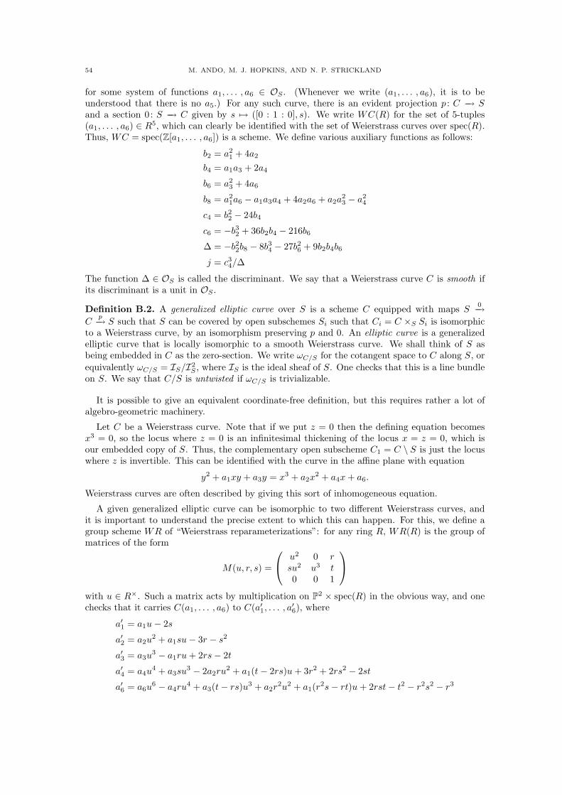
54 M. ANDO, M. J. HOPKINS, AND N. P. STRICKLAND
for some system of functions a1, . . . , a6 ∈ OS . (Whenever we write (a1, . . . , a6), it is to beunderstood that there is no a5.) For any such curve, there is an evident projection p : C −→ Sand a section 0: S −→ C given by s 7→ ([0 : 1 : 0], s). We write WC(R) for the set of 5-tuples(a1, . . . , a6) ∈ R5, which can clearly be identified with the set of Weierstrass curves over spec(R).Thus, WC = spec(Z[a1, . . . , a6]) is a scheme. We define various auxiliary functions as follows:
b2 = a21 + 4a2
b4 = a1a3 + 2a4
b6 = a23 + 4a6
b8 = a21a6 − a1a3a4 + 4a2a6 + a2a
23 − a2
4
c4 = b22 − 24b4
c6 = −b32 + 36b2b4 − 216b6
∆ = −b22b8 − 8b3
4 − 27b26 + 9b2b4b6
j = c34/∆
The function ∆ ∈ OS is called the discriminant. We say that a Weierstrass curve C is smooth ifits discriminant is a unit in OS .
Definition B.2. A generalized elliptic curve over S is a scheme C equipped with maps S0−→
Cp−→ S such that S can be covered by open subschemes Si such that Ci = C ×S Si is isomorphic
to a Weierstrass curve, by an isomorphism preserving p and 0. An elliptic curve is a generalizedelliptic curve that is locally isomorphic to a smooth Weierstrass curve. We shall think of S asbeing embedded in C as the zero-section. We write ωC/S for the cotangent space to C along S, orequivalently ωC/S = IS/I2
S , where IS is the ideal sheaf of S. One checks that this is a line bundleon S. We say that C/S is untwisted if ωC/S is trivializable.
It is possible to give an equivalent coordinate-free definition, but this requires rather a lot ofalgebro-geometric machinery.
Let C be a Weierstrass curve. Note that if we put z = 0 then the defining equation becomesx3 = 0, so the locus where z = 0 is an infinitesimal thickening of the locus x = z = 0, which isour embedded copy of S. Thus, the complementary open subscheme C1 = C \ S is just the locuswhere z is invertible. This can be identified with the curve in the affine plane with equation
y2 + a1xy + a3y = x3 + a2x2 + a4x + a6.
Weierstrass curves are often described by giving this sort of inhomogeneous equation.
A given generalized elliptic curve can be isomorphic to two different Weierstrass curves, andit is important to understand the precise extent to which this can happen. For this, we define agroup scheme WR of “Weierstrass reparameterizations”: for any ring R, WR(R) is the group ofmatrices of the form
M(u, r, s) =
u2 0 rsu2 u3 t0 0 1
with u ∈ R×. Such a matrix acts by multiplication on P2 × spec(R) in the obvious way, and onechecks that it carries C(a1, . . . , a6) to C(a′1, . . . , a′6), where
a′1 = a1u− 2s
a′2 = a2u2 + a1su− 3r − s2
a′3 = a3u3 − a1ru + 2rs− 2t
a′4 = a4u4 + a3su
3 − 2a2ru2 + a1(t− 2rs)u + 3r2 + 2rs2 − 2st
a′6 = a6u6 − a4ru
4 + a3(t− rs)u3 + a2r2u2 + a1(r2s− rt)u + 2rst− t2 − r2s2 − r3
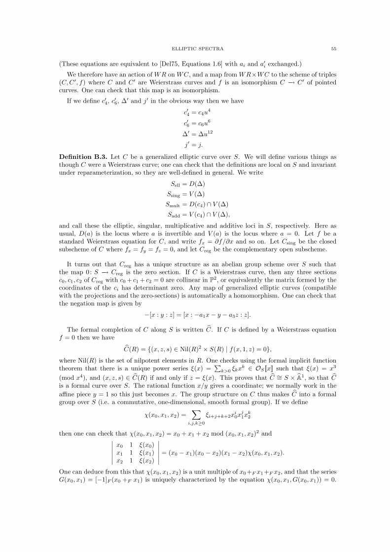
ELLIPTIC SPECTRA 55
(These equations are equivalent to [Del75, Equations 1.6] with ai and a′i exchanged.)
We therefore have an action of WR on WC, and a map from WR×WC to the scheme of triples(C, C ′, f) where C and C ′ are Weierstrass curves and f is an isomorphism C −→ C ′ of pointedcurves. One can check that this map is an isomorphism.
If we define c′4, c′6, ∆′ and j′ in the obvious way then we have
c′4 = c4u4
c′6 = c6u6
∆′ = ∆u12
j′ = j.
Definition B.3. Let C be a generalized elliptic curve over S. We will define various things asthough C were a Weierstrass curve; one can check that the definitions are local on S and invariantunder reparameterization, so they are well-defined in general. We write
Sell = D(∆)
Ssing = V (∆)
Smult = D(c4) ∩ V (∆)
Sadd = V (c4) ∩ V (∆),
and call these the elliptic, singular, multiplicative and additive loci in S, respectively. Here asusual, D(a) is the locus where a is invertible and V (a) is the locus where a = 0. Let f be astandard Weierstrass equation for C, and write fx = ∂f/∂x and so on. Let Csing be the closedsubscheme of C where fx = fy = fz = 0, and let Creg be the complementary open subscheme.
It turns out that Creg has a unique structure as an abelian group scheme over S such thatthe map 0: S −→ Creg is the zero section. If C is a Weierstrass curve, then any three sectionsc0, c1, c2 of Creg with c0 + c1 + c2 = 0 are collinear in P2, or equivalently the matrix formed by thecoordinates of the ci has determinant zero. Any map of generalized elliptic curves (compatiblewith the projections and the zero-sections) is automatically a homomorphism. One can check thatthe negation map is given by
−[x : y : z] = [x : −a1x− y − a3z : z].
The formal completion of C along S is written C. If C is defined by a Weierstrass equationf = 0 then we have
C(R) = (x, z, s) ∈ Nil(R)2 × S(R) | f(x, 1, z) = 0,where Nil(R) is the set of nilpotent elements in R. One checks using the formal implicit functiontheorem that there is a unique power series ξ(x) =
∑k>0 ξkxk ∈ OS [[x]] such that ξ(x) = x3
(mod x4), and (x, z, s) ∈ C(R) if and only if z = ξ(x). This proves that C ∼= S × A1, so that Cis a formal curve over S. The rational function x/y gives a coordinate; we normally work in theaffine piece y = 1 so this just becomes x. The group structure on C thus makes C into a formalgroup over S (i.e. a commutative, one-dimensional, smooth formal group). If we define
χ(x0, x1, x2) =∑
i,j,k≥0
ξi+j+k+2xi0x
j1x
k2
then one can check that χ(x0, x1, x2) = x0 + x1 + x2 mod (x0, x1, x2)2 and∣∣∣∣∣∣
x0 1 ξ(x0)x1 1 ξ(x1)x2 1 ξ(x2)
∣∣∣∣∣∣= (x0 − x1)(x0 − x2)(x1 − x2)χ(x0, x1, x2).
One can deduce from this that χ(x0, x1, x2) is a unit multiple of x0+F x1+F x2, and that the seriesG(x0, x1) = [−1]F (x0 +F x1) is uniquely characterized by the equation χ(x0, x1, G(x0, x1)) = 0.
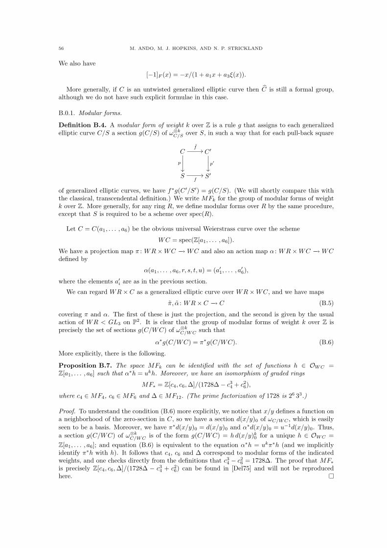
56 M. ANDO, M. J. HOPKINS, AND N. P. STRICKLAND
We also have
[−1]F (x) = −x/(1 + a1x + a3ξ(x)).
More generally, if C is an untwisted generalized elliptic curve then C is still a formal group,although we do not have such explicit formulae in this case.
B.0.1. Modular forms.
Definition B.4. A modular form of weight k over Z is a rule g that assigns to each generalizedelliptic curve C/S a section g(C/S) of ω⊗k
C/S over S, in such a way that for each pull-back square
Cf
//
p
²²
C ′
p′
²²
Sf
// S′
of generalized elliptic curves, we have f∗g(C ′/S′) = g(C/S). (We will shortly compare this withthe classical, transcendental definition.) We write MFk for the group of modular forms of weightk over Z. More generally, for any ring R, we define modular forms over R by the same procedure,except that S is required to be a scheme over spec(R).
Let C = C(a1, . . . , a6) be the obvious universal Weierstrass curve over the scheme
WC = spec(Z[a1, . . . , a6]).
We have a projection map π : WR×WC −→ WC and also an action map α : WR×WC −→ WCdefined by
α(a1, . . . , a6, r, s, t, u) = (a′1, . . . , a′6),
where the elements a′i are as in the previous section.
We can regard WR× C as a generalized elliptic curve over WR×WC, and we have maps
π, α : WR× C −→ C (B.5)
covering π and α. The first of these is just the projection, and the second is given by the usualaction of WR < GL3 on P2. It is clear that the group of modular forms of weight k over Z isprecisely the set of sections g(C/WC) of ω⊗k
C/WC such that
α∗g(C/WC) = π∗g(C/WC). (B.6)
More explicitly, there is the following.
Proposition B.7. The space MFk can be identified with the set of functions h ∈ OWC =Z[a1, . . . , a6] such that α∗h = ukh. Moreover, we have an isomorphism of graded rings
MF∗ = Z[c4, c6, ∆]/(1728∆− c34 + c2
6),
where c4 ∈ MF4, c6 ∈ MF6 and ∆ ∈ MF12. (The prime factorization of 1728 is 26 33.)
Proof. To understand the condition (B.6) more explicitly, we notice that x/y defines a function ona neighborhood of the zero-section in C, so we have a section d(x/y)0 of ωC/WC , which is easilyseen to be a basis. Moreover, we have π∗d(x/y)0 = d(x/y)0 and α∗d(x/y)0 = u−1d(x/y)0. Thus,a section g(C/WC) of ω⊗k
C/WC is of the form g(C/WC) = h d(x/y)k0 for a unique h ∈ OWC =
Z[a1, . . . , a6]; and equation (B.6) is equivalent to the equation α∗h = ukπ∗h (and we implicitlyidentify π∗h with h). It follows that c4, c6 and ∆ correspond to modular forms of the indicatedweights, and one checks directly from the definitions that c3
4 − c26 = 1728∆. The proof that MF∗
is precisely Z[c4, c6,∆]/(1728∆ − c34 + c2
6) can be found in [Del75] and will not be reproducedhere.
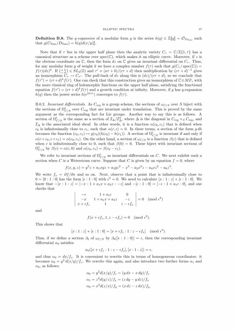
ELLIPTIC SPECTRA 57
Definition B.8. The q-expansion of a modular form g is the series h(q) ∈ Z[[q]] = ODTate suchthat g(CTate/DTate) = h(q)d(x/y)k
0 .
Note that if τ lies in the upper half plane then the analytic variety Cτ = C/Z1, τ has acanonical structure as a scheme over spec(C), which makes it an elliptic curve. Moreover, if z isthe obvious coordinate on C, then the form dz on C gives an invariant differential on Cτ . Thus,for any modular form g of weight k we have a complex number f(τ) such that g(Cτ/ spec(C)) =f(τ)(dz)k. If
(a bc d
) ∈ SL2(Z) and τ ′ = (aτ + b)/(cτ + d) then multiplication by (cτ + d)−1 givesan isomorphism Cτ −→ Cτ ′ . The pull-back of dz along this is (dz)/(cτ + d), so we conclude thatf(τ ′) = (cτ +d)kf(τ). One can check that this construction gives an isomorphism of C⊗MF∗ withthe more classical ring of holomorphic functions on the upper half plane, satisfying the functionalequation f(τ ′) = (cτ + d)kf(τ) and a growth condition at infinity. Moreover, if g has q-expansionh(q) then the power series h(e2πiτ ) converges to f(τ).
B.0.2. Invariant differentials. As Creg is a group scheme, the sections of ωC/S over S biject withthe sections of Ω1
C/S over Creg that are invariant under translation. This is proved by the sameargument as the corresponding fact for Lie groups. Another way to say this is as follows. Asection of Ω1
C/S is the same as a section of I∆/I2∆, where ∆ is the diagonal in Creg ×S Creg, and
I∆ is the associated ideal sheaf. In other words, it is a function α(c0, c1) that is defined whenc0 is infinitesimally close to c1, such that α(c, c) = 0. In these terms, a section of the form g dhbecomes the function (c0, c1) 7→ g(c0)(h(c0)− h(c1)). A section of Ω1
C/S is invariant if and only ifα(c+ c0, c+ c1) = α(c0, c1). On the other hand, a section of ωC/S is a function β(c) that is definedwhen c is infinitesimally close to 0, such that β(0) = 0. These biject with invariant sections ofΩ1
C/S by β(c) = α(c, 0) and α(c0, c1) = β(c0 − c1).
We refer to invariant sections of Ω1C/S as invariant differentials on C. We next exhibit such a
section when C is a Weierstrass curve. Suppose that C is given by an equation f = 0, where
f(x, y, z) = y2z + a1xyz + a3yz2 − x3 − a2x2z − a4xz2 − a6z
3.
We write fx = ∂f/∂x and so on. Next, observe that a point that is infinitesimally close to0 = [0 : 1 : 0] has the form [ε : 1 : 0] with ε2 = 0. We need to calculate [x : 1 : z] + [ε : 1 : 0]. Weknow that −[x : 1 : z] = [−x : 1 + a1x + a3z : −z] and −[ε : 1 : 0] = [−ε : 1 + a1ε : 0], and onechecks that ∣∣∣∣∣∣
−ε 1 + a1ε 0−x 1 + a1x + a3z −z
x + εfz 1 z − εfx
∣∣∣∣∣∣= 0 (mod ε2)
and
f(x + εfz, 1, z − εfx) = 0 (mod ε2).
This shows that
[x : 1 : z] + [ε : 1 : 0] = [x + εfz : 1 : z − εfx] (mod ε2).
Thus, if we define a section β0 of ωC/S by β0([ε : 1 : 0]) = ε, then the corresponding invariantdifferential α0 satisfies
α0([x + εfz : 1 : z − εfx], [x : 1 : z]) = ε,
and thus α0 = dx/fz. It is convenient to rewrite this in terms of homogeneous coordinates: itbecomes α0 = y2 d(x/y)/fz. We rewrite this again, and also introduce two further forms α1 andα2, as follows:
α0 = y2d(x/y)/fz = (y dx− x dy)/fz
α1 = z2d(y/z)/fx = (z dy − y dz)/fx
α2 = x2d(z/x)/fy = (x dz − z dx)/fy.
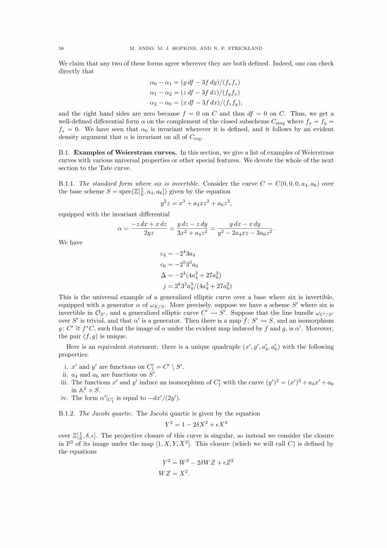
58 M. ANDO, M. J. HOPKINS, AND N. P. STRICKLAND
We claim that any two of these forms agree wherever they are both defined. Indeed, one can checkdirectly that
α0 − α1 = (y df − 3f dy)/(fxfz)
α1 − α2 = (z df − 3f dz)/(fyfx)
α2 − α0 = (x df − 3f dx)/(fzfy),
and the right hand sides are zero because f = 0 on C and thus df = 0 on C. Thus, we get awell-defined differential form α on the complement of the closed subscheme Csing where fx = fy =fz = 0. We have seen that α0 is invariant wherever it is defined, and it follows by an evidentdensity argument that α is invariant on all of Creg.
B.1. Examples of Weierstrass curves. In this section, we give a list of examples of Weierstrasscurves with various universal properties or other special features. We devote the whole of the nextsection to the Tate curve.
B.1.1. The standard form where six is invertible. Consider the curve C = C(0, 0, 0, a4, a6) overthe base scheme S = spec(Z[ 16 , a4, a6]) given by the equation
y2z = x3 + a4xz2 + a6z3,
equipped with the invariant differential
α =−z dx + x dz
2yz=
y dz − z dy
3x2 + a4z2=
y dx− x dy
y2 − 2a4xz − 3a6z2.
We have
c4 = −243a4
c6 = −2533a6
∆ = −24(4a34 + 27a2
6)
j = 2833a34/(4a3
4 + 27a26)
This is the universal example of a generalized elliptic curve over a base where six is invertible,equipped with a generator α of ωE/S . More precisely, suppose we have a scheme S′ where six isinvertible in OS′ , and a generalized elliptic curve C ′ −→ S′. Suppose that the line bundle ωC′/S′
over S′ is trivial, and that α′ is a generator. Then there is a map f : S′ −→ S, and an isomorphismg : C ′ ∼= f∗C, such that the image of α under the evident map induced by f and g, is α′. Moreover,the pair (f, g) is unique.
Here is an equivalent statement: there is a unique quadruple (x′, y′, a′4, a′6) with the following
properties:
i. x′ and y′ are functions on C ′1 = C ′ \ S′.ii. a4 and a6 are functions on S′.iii. The functions x′ and y′ induce an isomorphism of C ′1 with the curve (y′)2 = (x′)3 + a4x
′+ a6
in A2 × S.iv. The form α′|C′1 is equal to −dx′/(2y′).
B.1.2. The Jacobi quartic. The Jacobi quartic is given by the equation
Y 2 = 1− 2δX2 + εX4
over Z[ 16 , δ, ε]. The projective closure of this curve is singular, so instead we consider the closurein P3 of its image under the map [1, X, Y, X2]. This closure (which we will call C) is defined bythe equations
Y 2 = W 2 − 2δWZ + εZ2
WZ = X2.
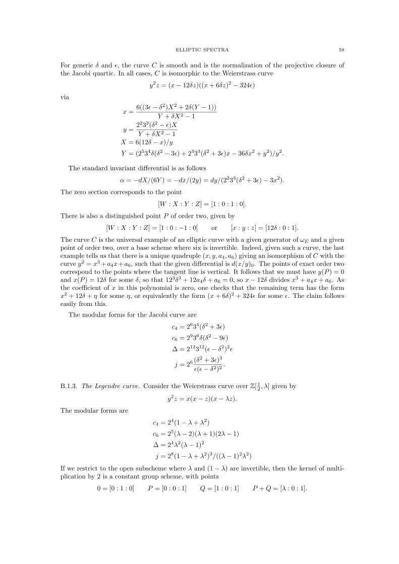
ELLIPTIC SPECTRA 59
For generic δ and ε, the curve C is smooth and is the normalization of the projective closure ofthe Jacobi quartic. In all cases, C is isomorphic to the Weierstrass curve
y2z = (x− 12δz)((x + 6δz)2 − 324ε)
via
x =6((3ε− δ2)X2 + 2δ(Y − 1))
Y + δX2 − 1
y =2233(δ2 − ε)XY + δX2 − 1
X = 6(12δ − x)/y
Y = (2534δ(δ2 − 3ε) + 2333(δ2 + 3ε)x− 36δx2 + y2)/y2.
The standard invariant differential is as follows
α = −dX/(6Y ) = −dx/(2y) = dy/(2233(δ2 + 3ε)− 3x2).
The zero section corresponds to the point
[W : X : Y : Z] = [1 : 0 : 1 : 0].
There is also a distinguished point P of order two, given by
[W : X : Y : Z] = [1 : 0 : −1 : 0] or [x : y : z] = [12δ : 0 : 1].
The curve C is the universal example of an elliptic curve with a given generator of ωE and a givenpoint of order two, over a base scheme where six is invertible. Indeed, given such a curve, the lastexample tells us that there is a unique quadruple (x, y, a4, a6) giving an isomorphism of C with thecurve y2 = x3 +a4x+a6, such that the given differential is d(x/y)0. The points of exact order twocorrespond to the points where the tangent line is vertical. It follows that we must have y(P ) = 0and x(P ) = 12δ for some δ, so that 123δ3 + 12a4δ + a6 = 0, so x− 12δ divides x3 + a4x + a6. Asthe coefficient of x in this polynomial is zero, one checks that the remaining term has the formx2 + 12δ + η for some η, or equivalently the form (x + 6δ)2 + 324ε for some ε. The claim followseasily from this.
The modular forms for the Jacobi curve are
c4 = 2634(δ2 + 3ε)
c6 = 2936δ(δ2 − 9ε)
∆ = 212312(ε− δ2)2ε
j = 26 (δ2 + 3ε)3
ε(ε− δ2)2.
B.1.3. The Legendre curve. Consider the Weierstrass curve over Z[ 12 , λ] given by
y2z = x(x− z)(x− λz).
The modular forms are
c4 = 24(1− λ + λ2)
c6 = 25(λ− 2)(λ + 1)(2λ− 1)
∆ = 24λ2(λ− 1)2
j = 28(1− λ + λ2)3/((λ− 1)2λ2)
If we restrict to the open subscheme where λ and (1− λ) are invertible, then the kernel of multi-plication by 2 is a constant group scheme, with points
0 = [0 : 1 : 0] P = [0 : 0 : 1] Q = [1 : 0 : 1] P + Q = [λ : 0 : 1].
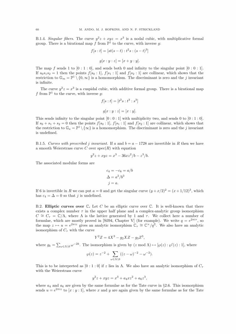
60 M. ANDO, M. J. HOPKINS, AND N. P. STRICKLAND
B.1.4. Singular fibers. The curve y2z + xyz = x3 is a nodal cubic, with multiplicative formalgroup. There is a birational map f from P1 to the curve, with inverse g:
f [s : t] = [st(s− t) : t2s : (s− t)3]
g[x : y : z] = [x + y : y].
The map f sends 1 to [0 : 1 : 0], and sends both 0 and infinity to the singular point [0 : 0 : 1].If s0s1s2 = 1 then the points f [s0 : 1], f [s1 : 1] and f [s2 : 1] are collinear, which shows that therestriction to Gm = P1 \ 0,∞ is a homomorphism. The discriminant is zero and the j invariantis infinite.
The curve y2z = x3 is a cuspidal cubic, with additive formal group. There is a birational mapf from P1 to the curve, with inverse g:
f [s : t] = [t2s : t3 : s3]
g[x : y : z] = [x : y].
This sends infinity to the singular point [0 : 0 : 1] with multiplicity two, and sends 0 to [0 : 1 : 0].If s0 + s1 + s2 = 0 then the points f [s0 : 1], f [s1 : 1] and f [s2 : 1] are collinear, which shows thatthe restriction to Ga = P1 \∞ is a homomorphism. The discriminant is zero and the j invariantis undefined.
B.1.5. Curves with prescribed j invariant. If a and b = a− 1728 are invertible in R then we havea smooth Weierstrass curve C over spec(R) with equation
y2z + xyz = x3 − 36xz2/b− z3/b.
The associated modular forms are
c4 = −c6 = a/b
∆ = a2/b3
j = a.
If 6 is invertible in R we can put a = 0 and get the singular curve (y +x/2)2 = (x+1/12)3, whichhas c4 = ∆ = 0 so that j is undefined.
B.2. Elliptic curves over C. Let C be an elliptic curve over C. It is well-known that thereexists a complex number τ in the upper half plane and a complex-analytic group isomorphismC ∼= Cτ = C/Λ, where Λ is the lattice generated by 1 and τ . We collect here a number offormulae, which are mostly proved in [Sil94, Chapter V] (for example). We write q = e2πiτ , sothe map z 7→ u = e2πiz gives an analytic isomorphism Cτ
∼= C×/qZ. We also have an analyticisomorphism of Cτ with the curve
Y 2Z = 4X3 − g2XZ − g3Z3,
where gk =∑
ω∈Λ\0 ω−2k. The isomorphism is given by (z mod Λ) 7→ [℘(z) : ℘′(z) : 1], where
℘(z) = z−2 +∑
ω∈Λ\0((z − ω)−2 − ω−2).
This is to be interpreted as [0 : 1 : 0] if z lies in Λ. We also have an analytic isomorphism of Cτ
with the Weierstrass curve
y2z + xyz = x3 + a4xz2 + a6z3,
where a4 and a6 are given by the same formulae as for the Tate curve in §2.6. This isomorphismsends u = e2πiz to [x : y : 1], where x and y are again given by the same formulae as for the Tate
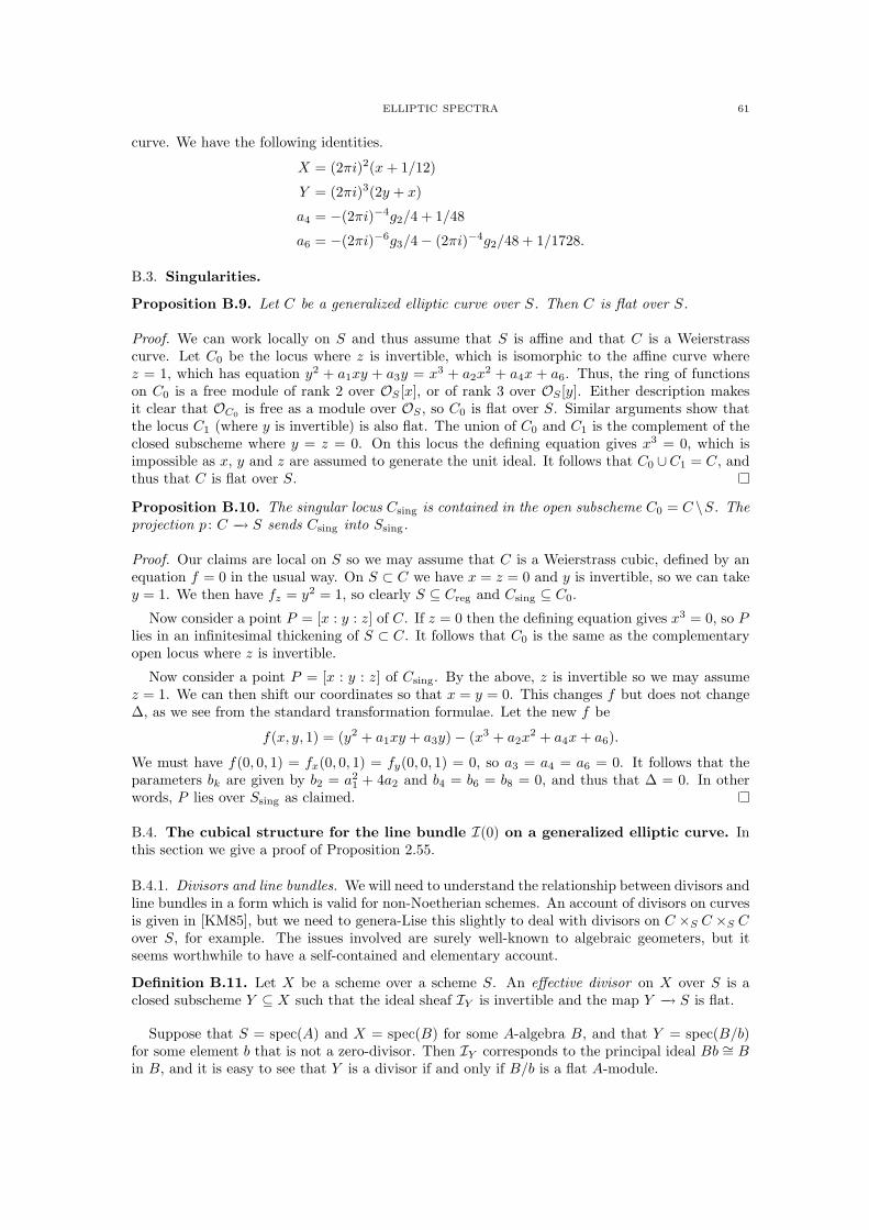
ELLIPTIC SPECTRA 61
curve. We have the following identities.
X = (2πi)2(x + 1/12)
Y = (2πi)3(2y + x)
a4 = −(2πi)−4g2/4 + 1/48
a6 = −(2πi)−6g3/4− (2πi)−4g2/48 + 1/1728.
B.3. Singularities.
Proposition B.9. Let C be a generalized elliptic curve over S. Then C is flat over S.
Proof. We can work locally on S and thus assume that S is affine and that C is a Weierstrasscurve. Let C0 be the locus where z is invertible, which is isomorphic to the affine curve wherez = 1, which has equation y2 + a1xy + a3y = x3 + a2x
2 + a4x + a6. Thus, the ring of functionson C0 is a free module of rank 2 over OS [x], or of rank 3 over OS [y]. Either description makesit clear that OC0 is free as a module over OS , so C0 is flat over S. Similar arguments show thatthe locus C1 (where y is invertible) is also flat. The union of C0 and C1 is the complement of theclosed subscheme where y = z = 0. On this locus the defining equation gives x3 = 0, which isimpossible as x, y and z are assumed to generate the unit ideal. It follows that C0 ∪C1 = C, andthus that C is flat over S.
Proposition B.10. The singular locus Csing is contained in the open subscheme C0 = C \S. Theprojection p : C −→ S sends Csing into Ssing.
Proof. Our claims are local on S so we may assume that C is a Weierstrass cubic, defined by anequation f = 0 in the usual way. On S ⊂ C we have x = z = 0 and y is invertible, so we can takey = 1. We then have fz = y2 = 1, so clearly S ⊆ Creg and Csing ⊆ C0.
Now consider a point P = [x : y : z] of C. If z = 0 then the defining equation gives x3 = 0, so Plies in an infinitesimal thickening of S ⊂ C. It follows that C0 is the same as the complementaryopen locus where z is invertible.
Now consider a point P = [x : y : z] of Csing. By the above, z is invertible so we may assumez = 1. We can then shift our coordinates so that x = y = 0. This changes f but does not change∆, as we see from the standard transformation formulae. Let the new f be
f(x, y, 1) = (y2 + a1xy + a3y)− (x3 + a2x2 + a4x + a6).
We must have f(0, 0, 1) = fx(0, 0, 1) = fy(0, 0, 1) = 0, so a3 = a4 = a6 = 0. It follows that theparameters bk are given by b2 = a2
1 + 4a2 and b4 = b6 = b8 = 0, and thus that ∆ = 0. In otherwords, P lies over Ssing as claimed.
B.4. The cubical structure for the line bundle I(0) on a generalized elliptic curve. Inthis section we give a proof of Proposition 2.55.
B.4.1. Divisors and line bundles. We will need to understand the relationship between divisors andline bundles in a form which is valid for non-Noetherian schemes. An account of divisors on curvesis given in [KM85], but we need to genera-Lise this slightly to deal with divisors on C ×S C ×S Cover S, for example. The issues involved are surely well-known to algebraic geometers, but itseems worthwhile to have a self-contained and elementary account.
Definition B.11. Let X be a scheme over a scheme S. An effective divisor on X over S is aclosed subscheme Y ⊆ X such that the ideal sheaf IY is invertible and the map Y −→ S is flat.
Suppose that S = spec(A) and X = spec(B) for some A-algebra B, and that Y = spec(B/b)for some element b that is not a zero-divisor. Then IY corresponds to the principal ideal Bb ∼= Bin B, and it is easy to see that Y is a divisor if and only if B/b is a flat A-module.
62 M. ANDO, M. J. HOPKINS, AND N. P. STRICKLAND
Conversely, if Y is a divisor then one can cover S by open sets of the form S′ = spec(A) andthe preimage X ′ of S′ by sets of the form spec(B) in such a way that Y ∩ spec(B) has the formspec(B/b) as above.
Proposition B.12. Let Y and Z be effective divisors on X over S. Then there is a uniqueeffective divisor Y + Z with IY +Z = IY IZ = IY ⊗OX
IZ . The effective divisors form an abelianmonoid Div+(X/S) under this operation. Moreover, this monoid has cancellation.
Proof. We define Y + Z to be the closed subscheme defined by the ideal sheaf IY IZ < OX . Weclaim that the product map IY ⊗OX
IZ −→ IY +Z = IY IZ is an isomorphism. Indeed, the questionis local, and locally it translates to the claim that Bb⊗B Bc maps isomorphically to Bbc when band c are not zero-divisors, and this claim is obvious. All that is left is to check that Y + Z is flatover S. Locally, we have a short exact sequence
B/b // c // B/bc // // B/c
with B/b and B/c flat over A, so B/bc is also flat over A. The rest is clear.
Definition B.13. We write Div(X/S) for the group completion of the monoid Div+(X/S), andrefer to its elements as divisors. The proposition implies that the natural map Div+(X/S) −→Div(X/S) is injective. It also implies that given a divisor Y = Y+ − Y−, we can define a linebundle IY = IY+I−1
Y− and this is well-defined up to canonical isomorphism.
Proposition B.14. Let f : X ′ −→ X be a flat map. Then the pull-back along f gives a homomor-phism Div+(X/S) −→ Div+(X ′/S), with If∗Y = f∗IY as line bundles over X ′. This extends togive an induced homomorphism f∗ : Div(X/S) −→ Div(X ′/S).
Proof. Let Y ⊂ X be a divisor, and write Y ′ = f∗Y = Y ×X X ′. It is clear that this is a closedsubscheme of X ′. The induced map f ′ : Y ′ −→ Y is a pull-back of a flat map so it is again flat.The map Y −→ S is flat because Y is a divisor, so the composite Y ′ −→ S is flat. Let j : Y −→ Xand j′ : Y ′ −→ X ′ be the inclusion maps. Essentially by definition we have f∗OX = OX′ andf∗j∗OY = j′∗(f ′)∗OY = j′∗OY ′ . We have a short exact sequence of sheaves IY −→ OX −→ j∗OY ,where j : Y −→ X is the inclusion. As f is flat, the functor f∗ is exact, so we have a short exactsequence f∗IY −→ OX′ −→ j′∗OY ′ . It follows that IY ′ = f∗IY , and f∗IY is clearly a line bundle.Thus, Y ′ is a divisor, as required. It is easy to see that f∗ is a homomorphism, and it follows bygeneral nonsense that it induces a map of group completions.
Proposition B.15. Let g : S′ −→ S be an arbitrary map, and write X ′ = g∗X. Then pull-backalong g gives a homomorphism Div+(X/S) −→ Div+(X ′/S′), with Ig∗Y = g∗IY as line bundlesover X ′. This extends to give an induced homomorphism f∗ : Div(X/S) −→ Div(X ′/S).
Proof. The proof is similar to that of the previous result.
Definition B.16. Let L be a line bundle over X, and u a section of L. Then there is a largestclosed subscheme Y of X such that u|Y = 0. If this is a divisor, we say that u is divisorial andwrite div(u) = Y . If so, then u is a trivialization of the line bundle L ⊗ IY , so L ∼= I−1
Y .
If v is a divisorial section of another line bundle M then one can check that u⊗ v is a divisorialsection of L ⊗M with div(u ⊗ v) = div(u) + div(v). One can also check that the formation ofdiv(u) is compatible with the two kinds of base change discussed in Propositions B.14 and B.15.
Definition B.17. A meromorphic divisorial section u of a line bundle L is an expression of theform u+/u−, where u+ and u− are divisorial sections of line bundles L+ and L− with a givenisomorphism L = L+/L−. These expressions are subject to the obvious sort of equivalence relation.We define div(u) = div(u+)−div(u−), which is well-defined by the above remarks. We again haveL ∼= I−1
div(u).
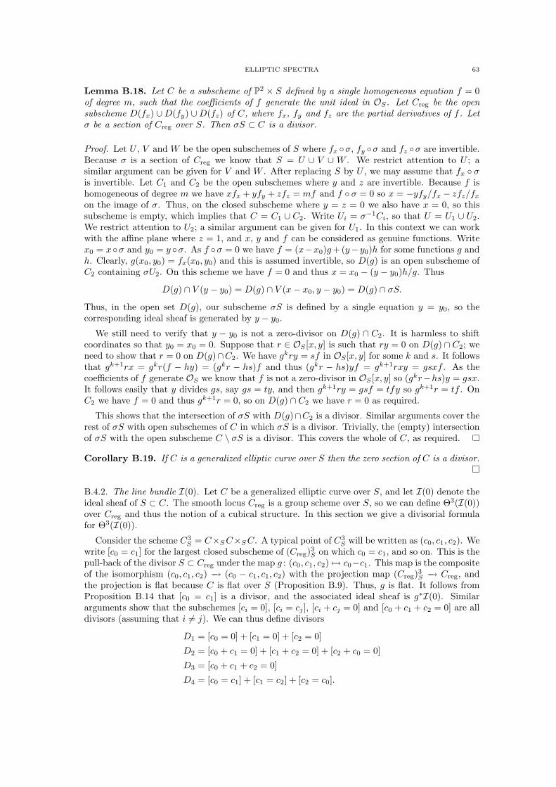
ELLIPTIC SPECTRA 63
Lemma B.18. Let C be a subscheme of P2 × S defined by a single homogeneous equation f = 0of degree m, such that the coefficients of f generate the unit ideal in OS. Let Creg be the opensubscheme D(fx) ∪D(fy) ∪D(fz) of C, where fx, fy and fz are the partial derivatives of f . Letσ be a section of Creg over S. Then σS ⊂ C is a divisor.
Proof. Let U , V and W be the open subschemes of S where fx σ, fy σ and fz σ are invertible.Because σ is a section of Creg we know that S = U ∪ V ∪ W . We restrict attention to U ; asimilar argument can be given for V and W . After replacing S by U , we may assume that fx σis invertible. Let C1 and C2 be the open subschemes where y and z are invertible. Because f ishomogeneous of degree m we have xfx + yfy + zfz = mf and f σ = 0 so x = −yfy/fx − zfz/fx
on the image of σ. Thus, on the closed subscheme where y = z = 0 we also have x = 0, so thissubscheme is empty, which implies that C = C1 ∪ C2. Write Ui = σ−1Ci, so that U = U1 ∪ U2.We restrict attention to U2; a similar argument can be given for U1. In this context we can workwith the affine plane where z = 1, and x, y and f can be considered as genuine functions. Writex0 = xσ and y0 = y σ. As f σ = 0 we have f = (x−x0)g +(y−y0)h for some functions g andh. Clearly, g(x0, y0) = fx(x0, y0) and this is assumed invertible, so D(g) is an open subscheme ofC2 containing σU2. On this scheme we have f = 0 and thus x = x0 − (y − y0)h/g. Thus
D(g) ∩ V (y − y0) = D(g) ∩ V (x− x0, y − y0) = D(g) ∩ σS.
Thus, in the open set D(g), our subscheme σS is defined by a single equation y = y0, so thecorresponding ideal sheaf is generated by y − y0.
We still need to verify that y − y0 is not a zero-divisor on D(g) ∩ C2. It is harmless to shiftcoordinates so that y0 = x0 = 0. Suppose that r ∈ OS [x, y] is such that ry = 0 on D(g) ∩ C2; weneed to show that r = 0 on D(g)∩C2. We have gkry = sf in OS [x, y] for some k and s. It followsthat gk+1rx = gkr(f − hy) = (gkr − hs)f and thus (gkr − hs)yf = gk+1rxy = gsxf . As thecoefficients of f generate OS we know that f is not a zero-divisor in OS [x, y] so (gkr−hs)y = gsx.It follows easily that y divides gs, say gs = ty, and then gk+1ry = gsf = tfy so gk+1r = tf . OnC2 we have f = 0 and thus gk+1r = 0, so on D(g) ∩ C2 we have r = 0 as required.
This shows that the intersection of σS with D(g)∩C2 is a divisor. Similar arguments cover therest of σS with open subschemes of C in which σS is a divisor. Trivially, the (empty) intersectionof σS with the open subscheme C \ σS is a divisor. This covers the whole of C, as required.
Corollary B.19. If C is a generalized elliptic curve over S then the zero section of C is a divisor.
B.4.2. The line bundle I(0). Let C be a generalized elliptic curve over S, and let I(0) denote theideal sheaf of S ⊂ C. The smooth locus Creg is a group scheme over S, so we can define Θ3(I(0))over Creg and thus the notion of a cubical structure. In this section we give a divisorial formulafor Θ3(I(0)).
Consider the scheme C3S = C×S C×S C. A typical point of C3
S will be written as (c0, c1, c2). Wewrite [c0 = c1] for the largest closed subscheme of (Creg)3S on which c0 = c1, and so on. This is thepull-back of the divisor S ⊂ Creg under the map g : (c0, c1, c2) 7→ c0−c1. This map is the compositeof the isomorphism (c0, c1, c2) −→ (c0 − c1, c1, c2) with the projection map (Creg)3S −→ Creg, andthe projection is flat because C is flat over S (Proposition B.9). Thus, g is flat. It follows fromProposition B.14 that [c0 = c1] is a divisor, and the associated ideal sheaf is g∗I(0). Similararguments show that the subschemes [ci = 0], [ci = cj ], [ci + cj = 0] and [c0 + c1 + c2 = 0] are alldivisors (assuming that i 6= j). We can thus define divisors
D1 = [c0 = 0] + [c1 = 0] + [c2 = 0]
D2 = [c0 + c1 = 0] + [c1 + c2 = 0] + [c2 + c0 = 0]
D3 = [c0 + c1 + c2 = 0]
D4 = [c0 = c1] + [c1 = c2] + [c2 = c0].
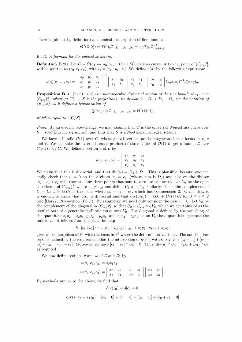
64 M. ANDO, M. J. HOPKINS, AND N. P. STRICKLAND
There is (almost by definition) a canonical isomorphism of line bundles
Θ3(I(0)) = I(0)0I−D1+D2−D3 = ωCID2I−1D1+D3
.
B.4.3. A formula for the cubical structure.
Definition B.20. Let C = C(a1, a2, a3, a4, a6) be a Weierstrass curve. A typical point of (Creg)3Swill be written as (c0, c1, c2), with ci = [xi : yi : zi]. We define s(a) by the following expression:
s(a)(c0, c1, c2) =
∣∣∣∣∣∣
x0 y0 z0
x1 y1 z1
x2 y2 z2
∣∣∣∣∣∣
−1 ∣∣∣∣x0 z0
x1 z1
∣∣∣∣∣∣∣∣
x1 z1
x2 z2
∣∣∣∣∣∣∣∣
x2 z2
x0 z0
∣∣∣∣ (z0z1z2)−1d(x/y)0.
Proposition B.21 (2.55). s(a) is a meromorphic divisorial section of the line bundle p∗ωC over(Creg)3S (where p : C3
S −→ S is the projection). Its divisor is −D1 + D2 − D3 (in the notation of§B.4.2), so it defines a trivialization of
(p∗ωC)⊗ I−D1+D2−D3 = Θ3(I(0)),
which is equal to s(C/S).
Proof. By an evident base-change, we may assume that C is the universal Weierstrass curve overS = spec(Z[a1, a2, a3, a4, a6]), and thus that S is a Noetherian, integral scheme.
We have a bundle O(1) over C, whose global sections are homogeneous linear forms in x, yand z. We can take the external tensor product of three copies of O(1) to get a bundle L overC ×S C ×S C. We define a section u of L by
u(c0, c1, c2) =
∣∣∣∣∣∣
x0 y0 z0
x1 y1 z1
x2 y2 z2
∣∣∣∣∣∣.
We claim that this is divisorial, and that div(u) = D4 + D3. This is plausible, because one caneasily check that u = 0 on the divisors [ci = cj ] (whose sum is D3) and also on the divisor[c0 + c1 + c2 = 0] (because any three points that sum to zero are collinear). Let U0 be the opensubscheme of (Creg)3S where c1 6= c2, and define U1 and U2 similarly. Then the complement ofU = U0 ∪ U1 ∪ U2 is the locus where c0 = c1 = c2, which has codimension 2. Given this, itis enough to check that u|Ui is divisorial and that div(u|Ui) = (D4 + D3) ∩ Ui for 0 ≤ i ≤ 2(see [Har77, Proposition II.6.5]). By symmetry, we need only consider the case i = 0. Let V0 bethe complement of the diagonal in (Creg)2S , so that U0 = Creg ×S V0, which we can think of as theregular part of a generalized elliptic curve over V0. The diagonal is defined by the vanishing ofthe quantities x1y2 − x2y1, y1z2 − y2z1, and z1x2 − z2x1, so on V0 these quantities generate theunit ideal. It follows from this that the map
h : [s1 : s2] 7→ [s1x1 + s2x2 : s1y1 + s2y2 : s1z1 + s2z2]
gives an isomorphism of P1 with the locus in P2 where the determinant vanishes. The addition lawon C is defined by the requirement that the intersection of h(P1) with C ×S V0 is [c0 = c1] + [c0 =c2] + [c0 = −c1 − c2]. Moreover, we have [c1 = c2] ∩ U0 = ∅. Thus, div(u) ∩ U0 = (D4 + D3) ∩ U0
as required.
We now define sections v and w of L and L2 by
v(c0, c1, c2) = z0z1z2
w(c0, c2, c2) =∣∣∣∣
x0 z0
x1 z1
∣∣∣∣∣∣∣∣
x1 z1
x2 z2
∣∣∣∣∣∣∣∣
x2 z2
x0 z0
∣∣∣∣ .
By methods similar to the above, we find that
div(z0) = 3[c0 = 0]
div(x0z1 − x1z0) = [c0 = 0] + [c1 = 0] + [c0 = c1] + [c0 + c1 = 0]
ELLIPTIC SPECTRA 65
and thus
div(v) = 3D1
div(w) = 2D1 + D2 + D4.
We also have s(a) = u−1wv−1d(x/y)0 so as claimed this is a meromorphic divisorial section ofp∗ωC , with divisor −D1 + D2 −D3. As explained earlier, it therefore gives rise to a trivializationof Θ3(I(0)).
Recall that Θ3(I(0)) is canonically trivialized on the locus where c2 = 0. In terms of ourpicture of Θ3(I(0)) involving rational one-forms, this isomorphism sends a one-form to its residueat c2 = 0. To calculate this for s(a), we may as well restrict attention to the affine piece wherey0 = y1 = y2 = 1, and let x2 tend to zero. The 3 × 3 determinant in the definition of s(a)approaches − | x0 z0
x1 z1 |. The defining cubic gives the relation
z2(1 + a1x2 − a2x22 + a3z2 − a4x2z2 − a6z
22) = x3
2,
which shows that z2 is asymptotic to x32 and thus that | x1 z1
x2 z2 | is asymptotic to −x2z1 and | x2 z2x0 z0 | is
asymptotic to x2z0. (Here we say that two functions f and g are asymptotic if there is a functionh on a neighborhood of the locus c2 = 0 such that f = gh and h = 1 when c2 = 0). It follows thats(a)(c0, c1, c2) is asymptotic to x−1
2 d(x)0, and this means that s(a) has residue 1, as required.
We now see that s(a) is a rigid section of Θ3(I(0)), so that f = s(a)/s(C/S) is an invertiblefunction on (Creg)3S , whose restriction to S is 1. It follows that f = 1 on the open subschemep−1Sell, which is dense in (Creg)3S , so f = 1 everywhere. Thus s(a) = s(C/S).
References
[ABS64] Michael F. Atiyah, Raoul Bott, and Arnold Shapiro. Clifford modules. Topology, 3 suppl. 1:3–38, 1964.[Ada76] J. Frank Adams. Primitive elements in the K-theory of BSU . Quart. J. Math. Oxford Ser. (2),
27(106):253–262, 1976.[Ada74] J. Frank Adams. Stable Homotopy and Generalised Homology. University of Chicago Press, Chicago,
1974.[AS98] Matthew Ando and Neil P. Strickland. Weil pairings and Morava K-theory. 23 pp., To appear in
Topology, 1998.[Bre83] L. Breen. Fonctions Theta et Theoreme du Cube, volume 980 of Lecture Notes in Mathematics.
Springer–Verlag, 1983.[BT89] Raoul Bott and Clifford Taubes. On the rigidity theorems of Witten. J. Amer. Math. Soc., 2(1):137–186,
1989.[Del75] Pierre Deligne. Courbes elliptiques: formulaire (d’apres J. Tate). In Modular Functions of One Variable
III, volume 476 of Lecture Notes in Mathematics, pages 53–73. Springer–Verlag, 1975.[Dem72] Michel Demazure. Lectures on p-divisible groups. Springer-Verlag, Berlin, 1972. Lecture Notes in Math-
ematics, Vol. 302.[DG70] Michel Demazure and Pierre Gabriel. Groupes algebriques. Tome I: Geometrie algebrique, generalites,
groupes commutatifs. Masson & Cie, Editeur, Paris, 1970. Avec un appendice Corps de classes localpar Michiel Hazewinkel.
[DR73] P. Deligne and M. Rapoport. Les schemas de modules de courbes elliptiques. In Modular Functions ofOne Variable II, volume 349 of Lecture Notes in Mathematics, pages 143–316. Springer–Verlag, 1973.
[EKMM96] A. D. Elmendorf, I. Kriz, M. A. Mandell, and J. P. May. Rings, Modules and Algebras in StableHomotopy Theory, volume 47 of Amer. Math. Soc. Surveys and Monographs. American MathematicalSociety, 1996.
[Fra92] J. Franke. On the construction of elliptic cohomology. Math. Nachr., 158:43–65, 1992.[FS80] G. Frobenius and L. Stickelberger. Uber die Addition und Multiplication der elliptischen Functionen.
J. fur die reine u. angewandte Math., 88:146–184, 1880. Reproduced in Frobenius, Oeuvres Completes,Springer 1968.
[Gro72] Groupes de monodromie en geometrie algebrique. I. Springer-Verlag, Berlin, 1972. Seminaire deGeometrie Algebrique du Bois-Marie 1967–1969 (SGA 7 I), Dirige par A. Grothendieck. Avec la col-laboration de M. Raynaud et D. S. Rim, Lecture Notes in Mathematics, Vol. 288.
[Har77] Robin H. Hartshorne. Algebraic Geometry, volume 52 of Graduate Texts in Mathematics. Springer–Verlag, 1977.
[Haz78] Michiel Hazewinkel. Formal Groups and Applications. Academic Press, 1978.
66 M. ANDO, M. J. HOPKINS, AND N. P. STRICKLAND
[HBJ92] Friedrich Hirzebruch, Thomas Berger, and Rainer Jung. Manifolds and modular forms. Aspects ofMathematics, E20. Friedr. Vieweg & Sohn, Braunschweig, 1992. With appendices by Nils-Peter Sko-ruppa and by Paul Baum.
[HM98] M. J. Hopkins and M. Mahowald. Elliptic curves and stable homotopy theory II. in preparation, 1998.[HMM98] M. J. Hopkins, M. Mahowald, and H. R. Miller. Elliptic curves and stable homotopy theory I. in
preparation, 1998.[Hop95] Michael J. Hopkins. Topological modular forms, the Witten genus, and the theorem of the cube. In
Proceedings of the International Congress of Mathematicians, Vol. 1, 2 (Zurich, 1994), pages 554–565,Basel, 1995. Birkhauser.
[Hus75] Dale Husemoller. Fibre Bundles, volume 33 of Graduate Texts in Mathematics. Springer–Verlag, 1975.[Jac] C. G. J. Jacobi. Formulae novae in theoria transcendentium ellipticarum fundamentales. Crelle J. fur
die reine u. angewandte Math., 15:199–204. Reproduced in Gesammelte Werke Vol. I 335-341, Verlagvon G. Reimer, Berlin 1881.
[Kat73] Nicholas M. Katz. p-adic properties of modular schemes and modular forms. In Modular functionsof one variable, III (Proc. Internat. Summer School, Univ. Antwerp, Antwerp, 1972), pages 69–190.Lecture Notes in Mathematics, Vol. 350, Berlin, 1973. Springer.
[KM85] N. M. Katz and B. Mazur. Arithmetic Moduli of Elliptic Curves, volume 108 of Annals of MathematicsStudies. Princeton University Press, 1985.
[Lan87] Serge Lang. Elliptic functions, volume 112 of Graduate Texts in Mathematics. Springer-Verlag, NewYork, second edition, 1987. With an appendix by J. Tate.
[Liu95] Kefeng Liu. On modular invariance and rigidity theorems. J. Differential Geom., 41(2):343–396, 1995.[LRS95] Peter S. Landweber, Douglas C. Ravenel, and Robert E. Stong. Periodic cohomology theories defined
by elliptic curves. In The Cech centennial (Boston, MA, 1993), volume 181 of Contemp. Math., pages317–337. Amer. Math. Soc., Providence, RI, 1995.
[MR81] Mark Mahowald and Nigel Ray. A note on the Thom isomorphism. Proc. Amer. Math. Soc., 82(2):307–308, 1981.
[MM65] John W. Milnor and John C. Moore. On the structure of Hopf algebras. Annals of Mathematics,81(2):211–264, 1965.
[Mor89] Jack Morava. Forms of K-theory. Math. Z., 201(3):401–428, 1989.[Mum65] David Mumford. Biextensions of formal groups. In Arithmetic algebraic geometry (proceedings of Pur-
due conference). Harper, 1965.[Mum70] David Mumford. Abelian Varieties, volume 5 of Tata institute of fundamental research series in math-
ematics. Oxford University Press, 1970.[Och87] S. Ochanine. Sur les genres multiplicatifs definis par des integrals elliptiques. Topology, 26:143–151,
1987.[Qui69] Daniel G. Quillen. On the formal group laws of unoriented and complex cobordism. Bulletin of the
American Mathematical Society, 75:1293–1298, 1969.[Qui71] Daniel G. Quillen. The spectrum of an equivariant cohomology ring, I and II. Annals of Mathematics,
94:549–602, 1971.[Ros98] Ioanid Rosu. Equivariant elliptic cohomology and rigidity. PhD thesis, MIT, 1998.[RW77] Douglas C. Ravenel and W. Stephen Wilson. The Hopf ring for complex cobordism. Journal of Pure
and Applied Algebra, 9:241–280, 1977.[Seg88] Graeme Segal. Elliptic cohomology. In Seminaire Bourbaki 1987/88, volume 161-162 of Asterisque,
pages 187–201. Societe Mathematique de France, Fevrier 1988.[Sil86] Joseph H. Silverman. The Arithmetic of Elliptic Curves. Graduate Texts in Mathematics. Springer–
Verlag, New York, 1986.[Sil94] Joseph H. Silverman. Advanced Topics in the Arithmetic of Elliptic Curves, volume 151 of Graduate
Texts in Mathematics. Springer–Verlag, New York, 1994.[Sin68] William M. Singer. Connective fiberings over BU and U . Topology, 7, 1968.[Str99a] Neil P. Strickland. Formal schemes and formal groups. In J.P. Meyer, J. Morava, and W.S. Wilson,
editors, Homotopy-invariant algebraic structures: in honor of J.M. Boardman, Contemporary Mathe-matics. American Mathematical Society, 1999. 75 pp., To Appear.
[Str99b] Neil P. Strickland. Products on MU -modules. Transactions of the American Mathematical Society,351:2569–2606, 1999.
[Tat74] John T. Tate. The arithmetic of elliptic curves. Invent. Math., 23:179–206, 1974.[Wit87] Edward Witten. Elliptic genera and quantum field theory. Comm. Math. Physics, 109:525–536, 1987.[Wit88] Edward Witten. The index of the Dirac operator in loop space. In P. S. Landweber, editor, Elliptic
Curves and Modular Forms in Algebraic Topology, volume 1326 of Lecture Notes in Mathematics, pages161–181, New York, 1988. Springer–Verlag.
ELLIPTIC SPECTRA 67
Department of Mathematics, The University of Illinois at Urbana-Champaign, Urbana IL 61801, USA
E-mail address: [email protected]
Department of Mathematics, Massachusetts Institute of Technology, Cambridge, MA 02139-4307,USA
E-mail address: [email protected]
Department of Pure Mathematics, University of Sheffield, Sheffield S3 7RH, England
E-mail address: [email protected]


![Vafa-Witten invariants of projective surfaces · Cumrun Vafa Ed Witten Riemannian 4-manifold M, SU(r) bundle E !M, connection A, elds B 2 +(su(E)); 2 0(su(E)), F+ A + [B:B] + [B;]](https://static.fdocument.org/doc/165x107/611a45e8ffc9dd3cfa5ceb98/vafa-witten-invariants-of-projective-surfaces-cumrun-vafa-ed-witten-riemannian-4-manifold.jpg)