An imbalanced Fermi gas in 1+ dimensions
38
An imbalanced Fermi gas in 1 + dimensions Andrew J. A. James A. Lamacraft 2009
Transcript of An imbalanced Fermi gas in 1+ dimensions
An imbalanced Fermi gas in 1 + ε dimensions
Andrew J. A. JamesA. Lamacraft
2009
Quantum Liquids
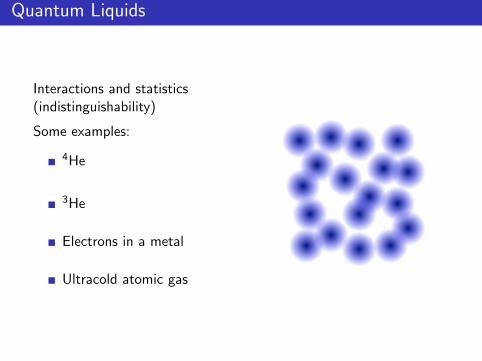
Interactions and statistics(indistinguishability)
Some examples:
4He
3He
Electrons in a metal
Ultracold atomic gas
Fermi Liquids
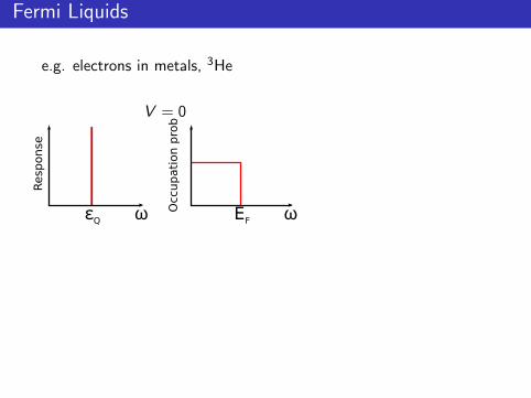
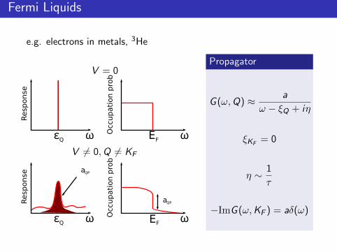
e.g. electrons in metals, 3He
V = 0
ωεQ ω
Resp
onse
Occ
upati
on p
rob
EF
V 6= 0,Q 6= KF
ωεQ ω
Resp
onse
Occ
upati
on p
rob
aQP
aQP
EF
Propagator
G (ω,Q) ≈ a
ω − ξQ + iη
ξKF= 0
η ∼ 1
τ
−ImG (ω,KF ) = aδ(ω)
Fermi Liquids
e.g. electrons in metals, 3He
V = 0
ωεQ ω
Resp
onse
Occ
upati
on p
rob
EF
V 6= 0,Q 6= KF
ωεQ ω
Resp
onse
Occ
upati
on p
rob
aQP
aQP
EF
Propagator
G (ω,Q) ≈ a
ω − ξQ + iη
ξKF= 0
η ∼ 1
τ
−ImG (ω,KF ) = aδ(ω)
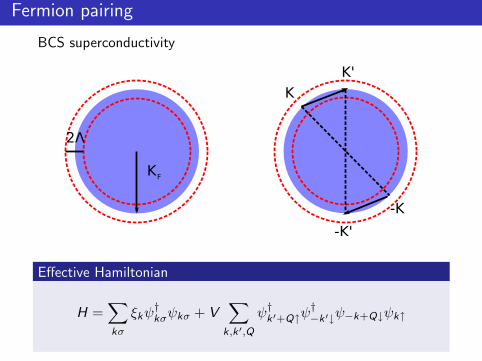
Fermion pairing
BCS superconductivity
2Λ
KF
K'
-K'
K
-K
Effective Hamiltonian
H =∑kσ
ξkψ†kσψkσ + V
∑k,k ′,Q
ψ†k ′+Q↑ψ
†−k ′↓ψ−k+Q↓ψk↑
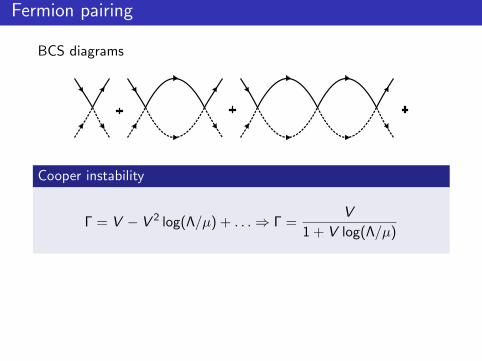
Fermion pairing
BCS diagrams
Cooper instability
Γ = V − V 2 log(Λ/µ) + . . .⇒ Γ =V
1 + V log(Λ/µ)
RG flow
dΓ
d log Λ= 0⇒ − dV
d log Λ= −V 2 V0
FLBCS
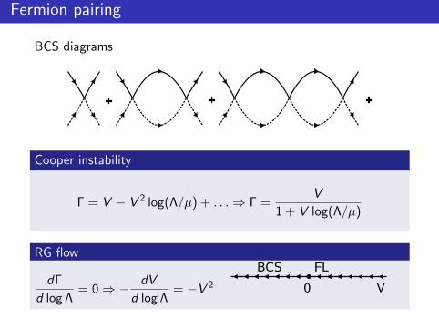
Fermion pairing
BCS diagrams
Cooper instability
Γ = V − V 2 log(Λ/µ) + . . .⇒ Γ =V
1 + V log(Λ/µ)
RG flow
dΓ
d log Λ= 0⇒ − dV
d log Λ= −V 2 V0
FLBCS
Inhomogenous Superconductors
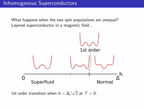
What happens when the two spin populations are unequal?Layered superconductor in a magnetic field...
h0 Δ
Superfluid Normal
1st order
1st order transition when h = ∆/√
2 at T = 0.
Inhomogenous Superconductors
What happens when the two spin populations are unequal?Layered superconductor in a magnetic field...
h0 Δ
Superfluid Normal
1st order
1st order transition when h = ∆/√
2 at T = 0.
Cooper’s Problem
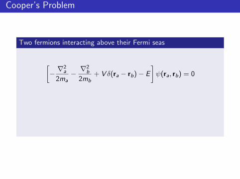
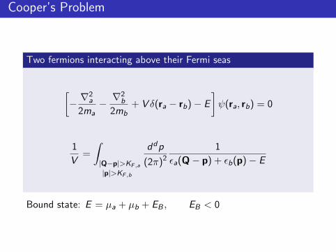
Two fermions interacting above their Fermi seas
[− ∇
2a
2ma−∇2
b
2mb+ V δ(ra − rb)− E
]ψ(ra, rb) = 0
1
V=
∫|Q−p|>KF ,a
|p|>KF ,b
ddp
(2π)21
εa(Q− p) + εb(p)− E
Bound state: E = µa + µb + EB , EB < 0
Cooper’s Problem
Two fermions interacting above their Fermi seas
[− ∇
2a
2ma−∇2
b
2mb+ V δ(ra − rb)− E
]ψ(ra, rb) = 0
1
V=
∫|Q−p|>KF ,a
|p|>KF ,b
ddp
(2π)21
εa(Q− p) + εb(p)− E
Bound state: E = µa + µb + EB , EB < 0
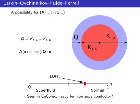
Larkin–Ovchinnikov–Fulde–Ferrell
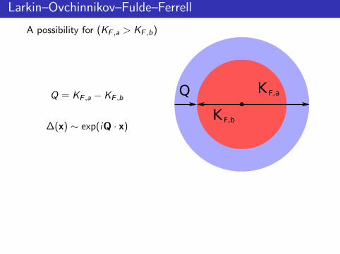
A possibility for (KF ,a > KF ,b)
Q = KF ,a − KF ,b
∆(x) ∼ exp(iQ · x)
Q KF,a
K F,b
h0 1
Superfluid Normal
LOFF
Seen in CeCoIn5, heavy fermion superconductor?
Larkin–Ovchinnikov–Fulde–Ferrell
A possibility for (KF ,a > KF ,b)
Q = KF ,a − KF ,b
∆(x) ∼ exp(iQ · x)
Q KF,a
K F,b
h0 1
Superfluid Normal
LOFF
Seen in CeCoIn5, heavy fermion superconductor?
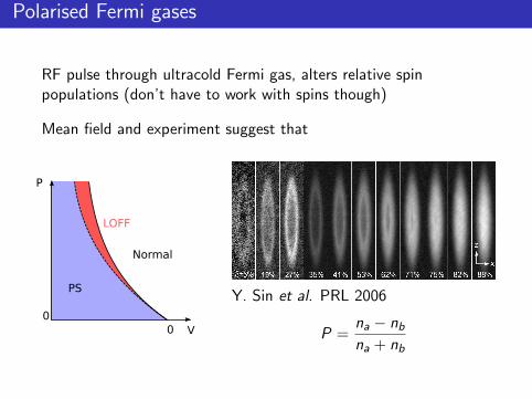
Polarised Fermi gases
RF pulse through ultracold Fermi gas, alters relative spinpopulations (don’t have to work with spins though)
Mean field and experiment suggest that
P
V0
LOFF
PS
Normal
0
Y. Sin et al. PRL 2006
P =na − nb
na + nb
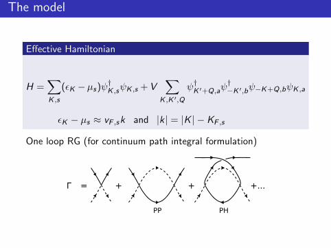
The model
Effective Hamiltonian
H =∑K ,s
(εK −µs)ψ†K ,sψK ,s +V
∑K ,K ′,Q
ψ†K ′+Q,aψ
†−K ′,bψ−K+Q,bψK ,a
εK − µs ≈ vF ,sk and |k| = |K | − KF ,s
One loop RG (for continuum path integral formulation)
PP PH
+ +Γ = +...
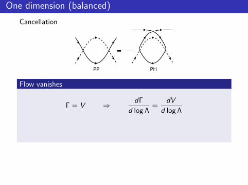
One dimension (balanced)
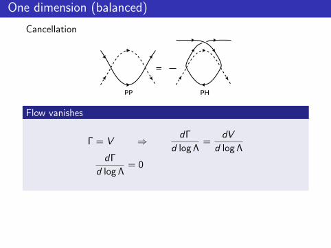
Cancellation
PP PH
=
Flow vanishes
Γ = V ⇒ dΓ
d log Λ=
dV
d log Λ
dΓ
d log Λ= 0 ⇒ β(V ) = 0
Cancellation occurs to all orders, (Ward identities, bosonization,exact solution of XXZ spin chain)Luttinger liquid, power law behaviour with interaction dependentexponents
One dimension (balanced)
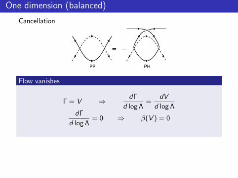
Cancellation
PP PH
=
Flow vanishes
Γ = V ⇒ dΓ
d log Λ=
dV
d log ΛdΓ
d log Λ= 0
⇒ β(V ) = 0
Cancellation occurs to all orders, (Ward identities, bosonization,exact solution of XXZ spin chain)Luttinger liquid, power law behaviour with interaction dependentexponents
One dimension (balanced)
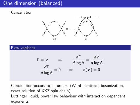
Cancellation
PP PH
=
Flow vanishes
Γ = V ⇒ dΓ
d log Λ=
dV
d log ΛdΓ
d log Λ= 0 ⇒ β(V ) = 0
Cancellation occurs to all orders, (Ward identities, bosonization,exact solution of XXZ spin chain)Luttinger liquid, power law behaviour with interaction dependentexponents
One dimension (balanced)
Cancellation
PP PH
=
Flow vanishes
Γ = V ⇒ dΓ
d log Λ=
dV
d log ΛdΓ
d log Λ= 0 ⇒ β(V ) = 0
Cancellation occurs to all orders, (Ward identities, bosonization,exact solution of XXZ spin chain)Luttinger liquid, power law behaviour with interaction dependentexponents
One + ε dimensions
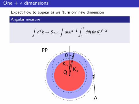
Expect flow to appear as we ‘turn on’ new dimension
Angular measure∫ddk→ Sd−1
∫dkkd−1
∫ π
0dθ(sin θ)d−2
QKa
Kb
PP
Λ
θ
One + ε dimensions
Expect flow to appear as we ‘turn on’ new dimension
Angular measure∫ddk→ Sd−1
∫dkkd−1
∫ π
0dθ(sin θ)d−2
QKa
Kb
PP
Λ
θ
One + ε dimensions
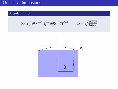
Angular cut off
Sd−1
∫dkkd−1
∫ θM
0 dθ(sin θ)d−2 θM ≈√
2KF ,akQKF ,b
Λ
θ
Γ in 1 + ε
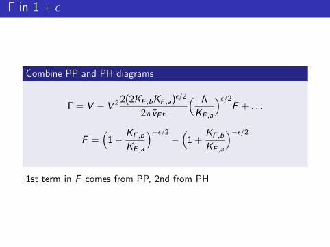
Combine PP and PH diagrams
Γ = V − V 2 2(2KF ,bKF ,a)ε/2
2πvF ε
( Λ
KF ,a
)ε/2F + . . .
F =(1−
KF ,b
KF ,a
)−ε/2−
(1 +
KF ,b
KF ,a
)−ε/2
1st term in F comes from PP, 2nd from PH
Flow and Fixed Point
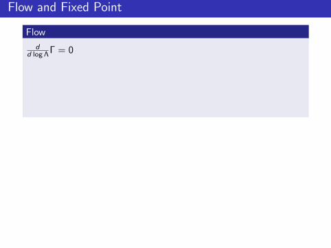
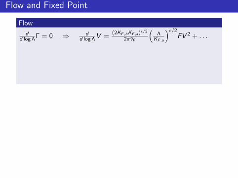
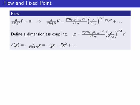
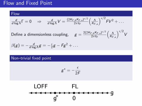
Flow
dd log ΛΓ = 0
⇒ dd log ΛV =
(2KF ,bKF ,a)ε/2
2πvF
(Λ
KF ,a
)ε/2FV 2 + . . .
Define a dimensionless coupling, g =2(2KF ,bKF ,a)
ε/2
2πvF
(Λ
KF ,a
)ε/2V
β(g) = − dd log Λg = − ε
2g − Fg2 + . . .
Non–trivial fixed point
g? = − ε
2F
g0g*
LOFF FL
Flow and Fixed Point
Flow
dd log ΛΓ = 0 ⇒ d
d log ΛV =(2KF ,bKF ,a)
ε/2
2πvF
(Λ
KF ,a
)ε/2FV 2 + . . .
Define a dimensionless coupling, g =2(2KF ,bKF ,a)
ε/2
2πvF
(Λ
KF ,a
)ε/2V
β(g) = − dd log Λg = − ε
2g − Fg2 + . . .
Non–trivial fixed point
g? = − ε
2F
g0g*
LOFF FL
Flow and Fixed Point
Flow
dd log ΛΓ = 0 ⇒ d
d log ΛV =(2KF ,bKF ,a)
ε/2
2πvF
(Λ
KF ,a
)ε/2FV 2 + . . .
Define a dimensionless coupling, g =2(2KF ,bKF ,a)
ε/2
2πvF
(Λ
KF ,a
)ε/2V
β(g) = − dd log Λg = − ε
2g − Fg2 + . . .
Non–trivial fixed point
g? = − ε
2F
g0g*
LOFF FL
Flow and Fixed Point
Flow
dd log ΛΓ = 0 ⇒ d
d log ΛV =(2KF ,bKF ,a)
ε/2
2πvF
(Λ
KF ,a
)ε/2FV 2 + . . .
Define a dimensionless coupling, g =2(2KF ,bKF ,a)
ε/2
2πvF
(Λ
KF ,a
)ε/2V
β(g) = − dd log Λg = − ε
2g − Fg2 + . . .
Non–trivial fixed point
g? = − ε
2F
g0g*
LOFF FL
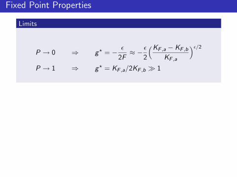
Fixed Point Properties
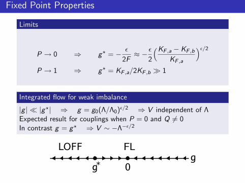
Limits
P → 0 ⇒ g? = − ε
2F≈ − ε
2
(KF ,a − KF ,b
KF ,a
)ε/2
P → 1 ⇒ g? = KF ,a/2KF ,b 1
Integrated flow for weak imbalance
|g | |g?| ⇒ g = g0(Λ/Λ0)ε/2 ⇒ V independent of Λ
Expected result for couplings when P = 0 and Q 6= 0In contrast g = g? ⇒ V ∼ −Λ−ε/2
g0g*
LOFF FL
Fixed Point Properties
Limits
P → 0 ⇒ g? = − ε
2F≈ − ε
2
(KF ,a − KF ,b
KF ,a
)ε/2
P → 1 ⇒ g? = KF ,a/2KF ,b 1
Integrated flow for weak imbalance
|g | |g?| ⇒ g = g0(Λ/Λ0)ε/2 ⇒ V independent of Λ
Expected result for couplings when P = 0 and Q 6= 0In contrast g = g? ⇒ V ∼ −Λ−ε/2
g0g*
LOFF FL
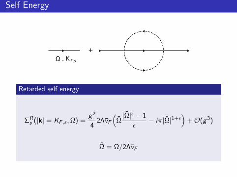
Self Energy
Ω , K F,s
+
Retarded self energy
ΣRs (|k| = KF ,s ,Ω) =
g2
42ΛvF
(Ω|Ω|ε − 1
ε− iπ|Ω|1+ε
)+O(g3)
Ω = Ω/2ΛvF
Propagator and Residue
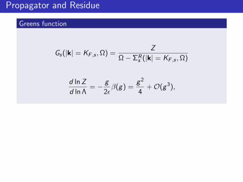
Greens function
Gs(|k| = KF ,s ,Ω) =Z
Ω− ΣRs (|k| = KF ,s ,Ω)
d lnZ
d ln Λ= − g
2εβ(g) =
g2
4+O(g3),
At the fixed point
No pole! Residue has vanished
Gs(|k| = KF ,s ,Ω) ∼ ωη−1,
η = ε2/16F 2
ω
Response
0
ωη-1
Propagator and Residue
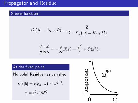
Greens function
Gs(|k| = KF ,s ,Ω) =Z
Ω− ΣRs (|k| = KF ,s ,Ω)
d lnZ
d ln Λ= − g
2εβ(g) =
g2
4+O(g3),
At the fixed point
No pole! Residue has vanished
Gs(|k| = KF ,s ,Ω) ∼ ωη−1,
η = ε2/16F 2
ω
Response
0
ωη-1
Residue
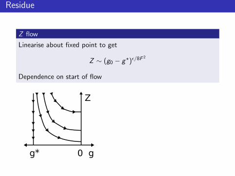
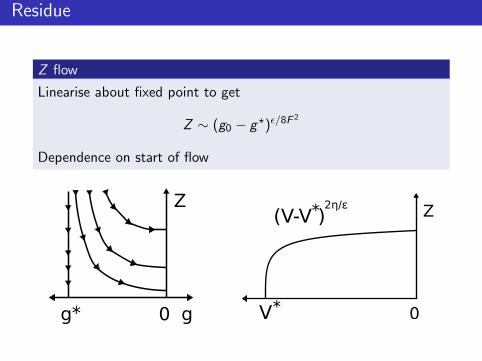
Z flow
Linearise about fixed point to get
Z ∼ (g0 − g?)ε/8F 2
Dependence on start of flow
g0g
Z
*
Z
0
(V-V )2η/ε
V*
*
Residue
Z flow
Linearise about fixed point to get
Z ∼ (g0 − g?)ε/8F 2
Dependence on start of flow
g0g
Z
*
Z
0
(V-V )2η/ε
V*
*
Two Species, with Spin
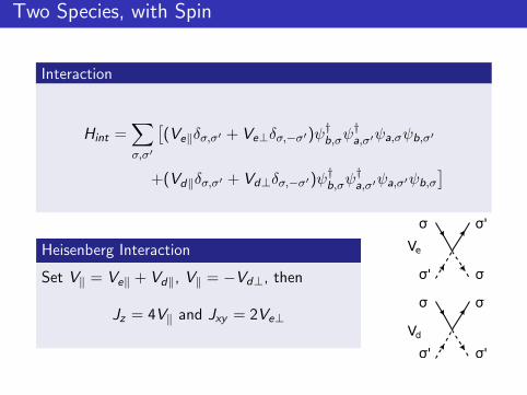
Interaction
Hint =∑σ,σ′
[(Ve‖δσ,σ′ + Ve⊥δσ,−σ′)ψ†
b,σψ†a,σ′ψa,σψb,σ′
+(Vd‖δσ,σ′ + Vd⊥δσ,−σ′)ψ†b,σψ
†a,σ′ψa,σ′ψb,σ
]
Heisenberg Interaction
Set V‖ = Ve‖ + Vd‖, V‖ = −Vd⊥, then
Jz = 4V‖ and Jxy = 2Ve⊥
σ'
σ
σ
σ'
σ
σ'
σ
σ'
Ve
Vd
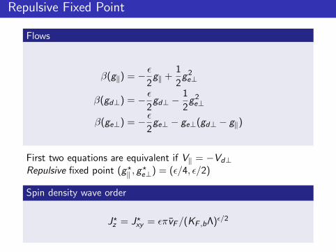
Repulsive Fixed Point
Flows
β(g‖) = − ε2g‖ +
1
2g2e⊥
β(gd⊥) = − ε2gd⊥ −
1
2g2e⊥
β(ge⊥) = − ε2ge⊥ − ge⊥(gd⊥ − g‖)
First two equations are equivalent if V‖ = −Vd⊥Repulsive fixed point (g?
‖ , g?e⊥) = (ε/4, ε/2)
Spin density wave order
J?z = J?
xy = επvF/(KF ,bΛ)ε/2
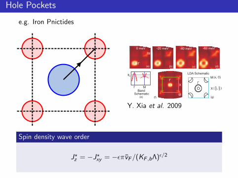
Hole Pockets
e.g. Iron Pnictides
0 meV -20 meV -40 meV -60 meV
(a) (b) (c) (d)
Γ
M
X
LDA Schematic
(f)
Γ
M
X
( , 0)π
( , )π
2π
2Γ M
(e)
Γ
M
EF
(g)
BandSchematic
Y. Xia et al. 2009
Spin density wave order
J?z = −J?
xy = −επvF/(KF ,bΛ)ε/2
Summary
RG flow for imbalanced Fermi gas in d = 1 + ε
Spinless case
Finite momentum pairingVanishing residue at fixed pointImbalance dependent critical exponent
Spinful cases, SDW order