9. Fermi Surfaces and Metals Construction of Fermi Surfaces Electron Orbits, Hole Orbits, and Open...
35
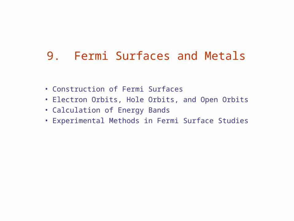
9. Fermi Surfaces and Metals • Construction of Fermi Surfaces • Electron Orbits, Hole Orbits, and Open Orbits • Calculation of Energy Bands • Experimental Methods in Fermi Surface Studies
-
Upload
hilda-clark -
Category
Documents
-
view
364 -
download
25
Transcript of 9. Fermi Surfaces and Metals Construction of Fermi Surfaces Electron Orbits, Hole Orbits, and Open...
9. Fermi Surfaces and Metals
• Construction of Fermi Surfaces
• Electron Orbits, Hole Orbits, and Open Orbits
• Calculation of Energy Bands
• Experimental Methods in Fermi Surface Studies
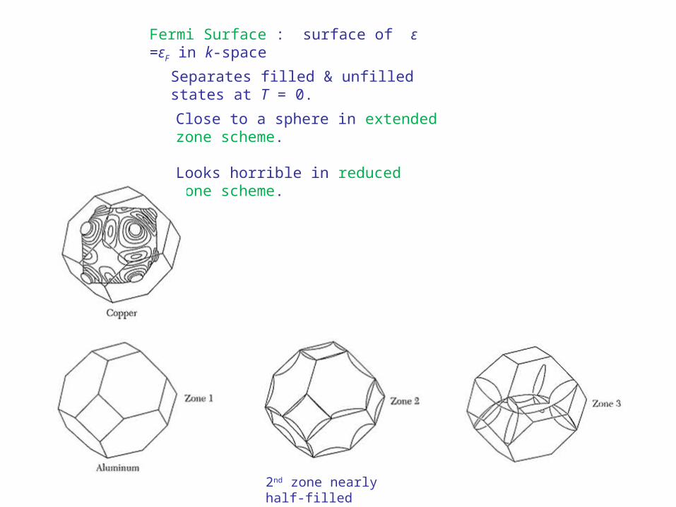
Fermi Surface : surface of ε =εF in k-space
Separates filled & unfilled states at T = 0.
Close to a sphere in extended zone scheme.
Looks horrible in reduced zone scheme.
2nd zone nearly half-filled
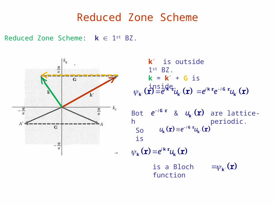
Reduced Zone Scheme
Reduced Zone Scheme: k 1st BZ.
k is outside 1st BZ.k = k + G is inside.
ie u k r
k kr r i ie e u k r G r
k r
ie u k rk kr r
k r
iu e u G r
k kr r
Both ie G r u k r& are lattice-periodic.
So is
→
is a Bloch function
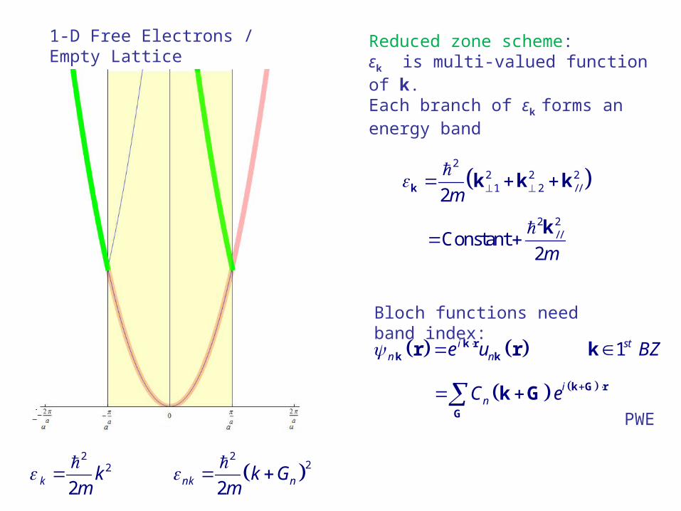
1-D Free Electrons / Empty Lattice
2
2 2 21 2 / /2m
k k k k
2 2/ /Constant
2m
k
Reduced zone scheme:εk is multi-valued function of k.Each branch of εk forms an energy band
Bloch functions need band index:
in ne u k r
k kr r 1st BZk
2
2
2nk nk Gm
inC e k G r
G
k GPWE
22
2k km
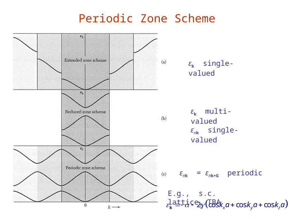
Periodic Zone Scheme
εk single-valued
εk multi-valuedεnk single-valued
εnk = εnk+G periodic
2 cos cos cosx y zk a k a k a k
E.g., s.c. lattice, TBA
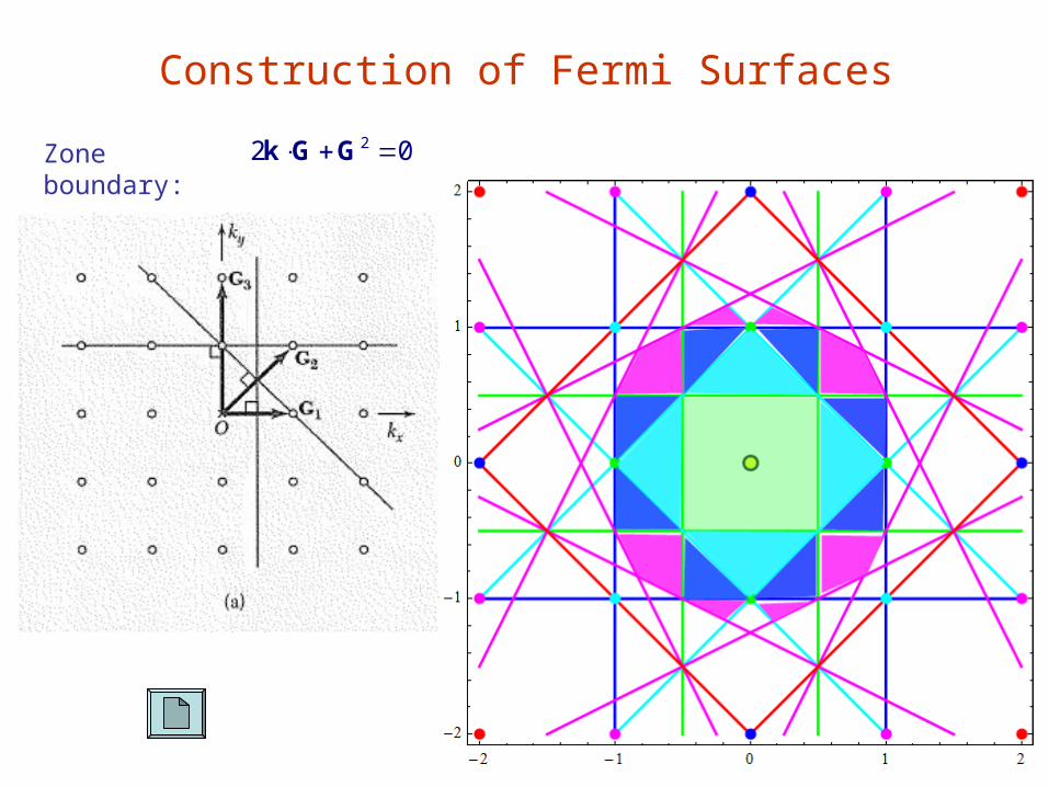
Construction of Fermi Surfaces
Zone boundary:22 0 G Gk
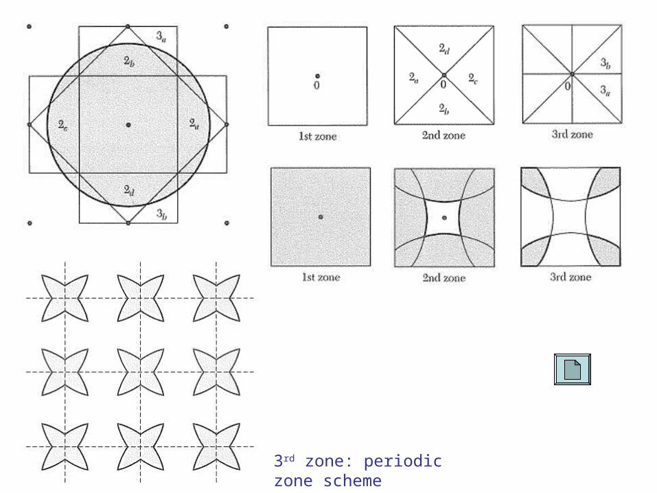
3rd zone: periodic zone scheme
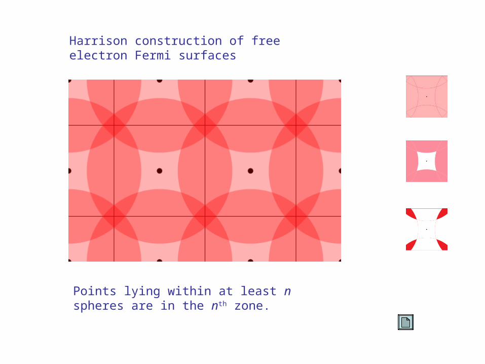
Harrison construction of free electron Fermi surfaces
Points lying within at least n spheres are in the nth zone.
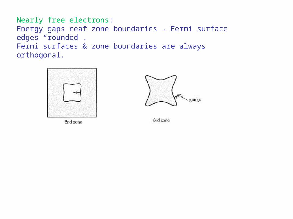
Nearly free electrons:Energy gaps near zone boundaries → Fermi surface edges “rounded”.Fermi surfaces & zone boundaries are always orthogonal.
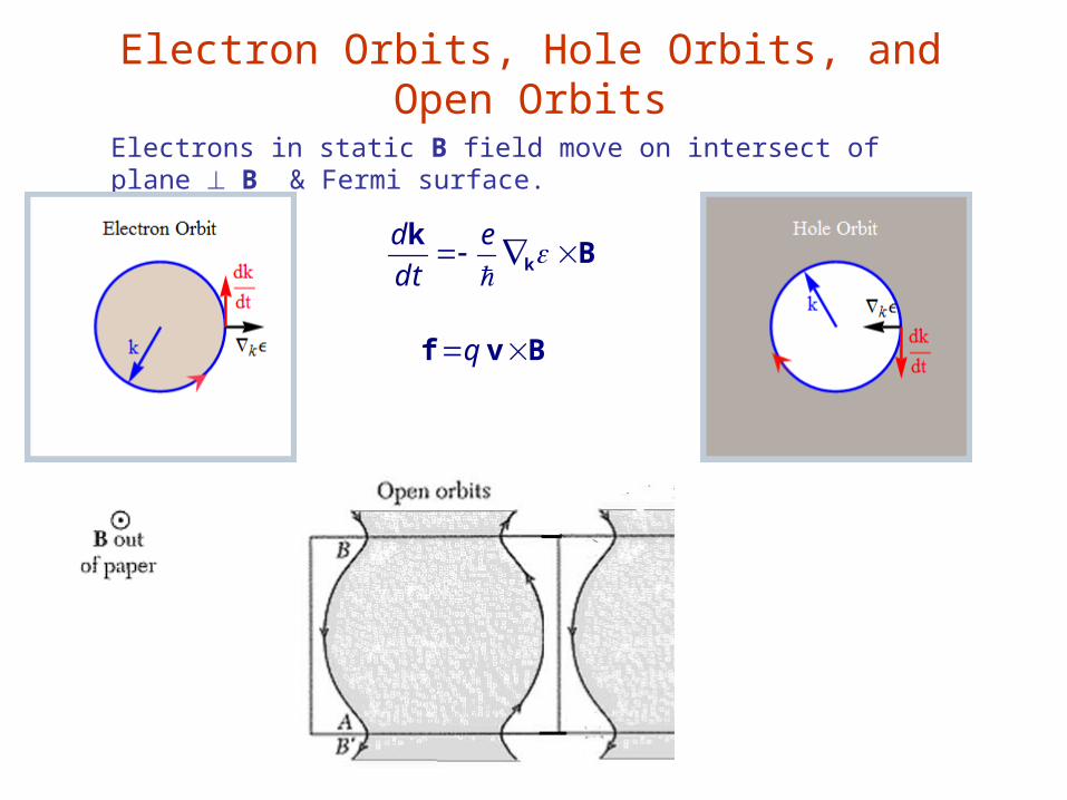
Electron Orbits, Hole Orbits, and Open Orbits
Electrons in static B field move on intersect of plane B & Fermi surface.
d e
dt k
kB
q f v B
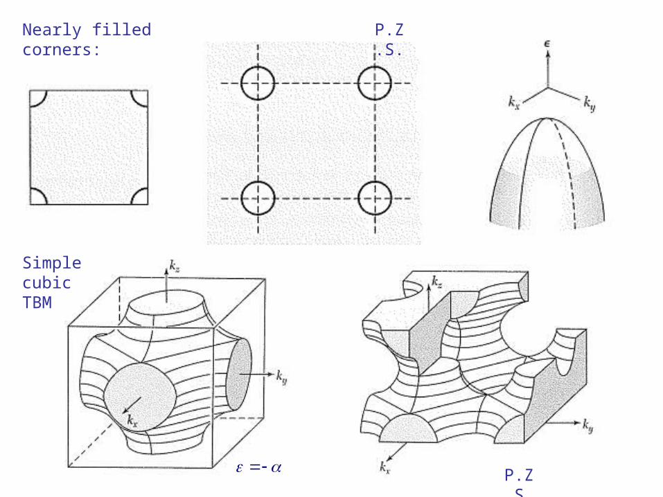
Nearly filled corners:
P.Z.S.
P.Z.S.
Simple cubicTBM
Calculation of Energy Bands
• Tight Binding Method for Energy Bands
• Wigner-Seitz Method
• Cohesive Energy
• Pseudopotential Methods
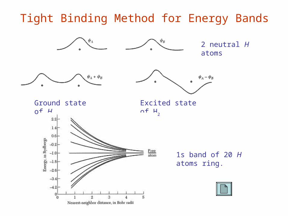
Tight Binding Method for Energy Bands
2 neutral H atoms
Ground state of H2 Excited state of H2
1s band of 20 H atoms ring.
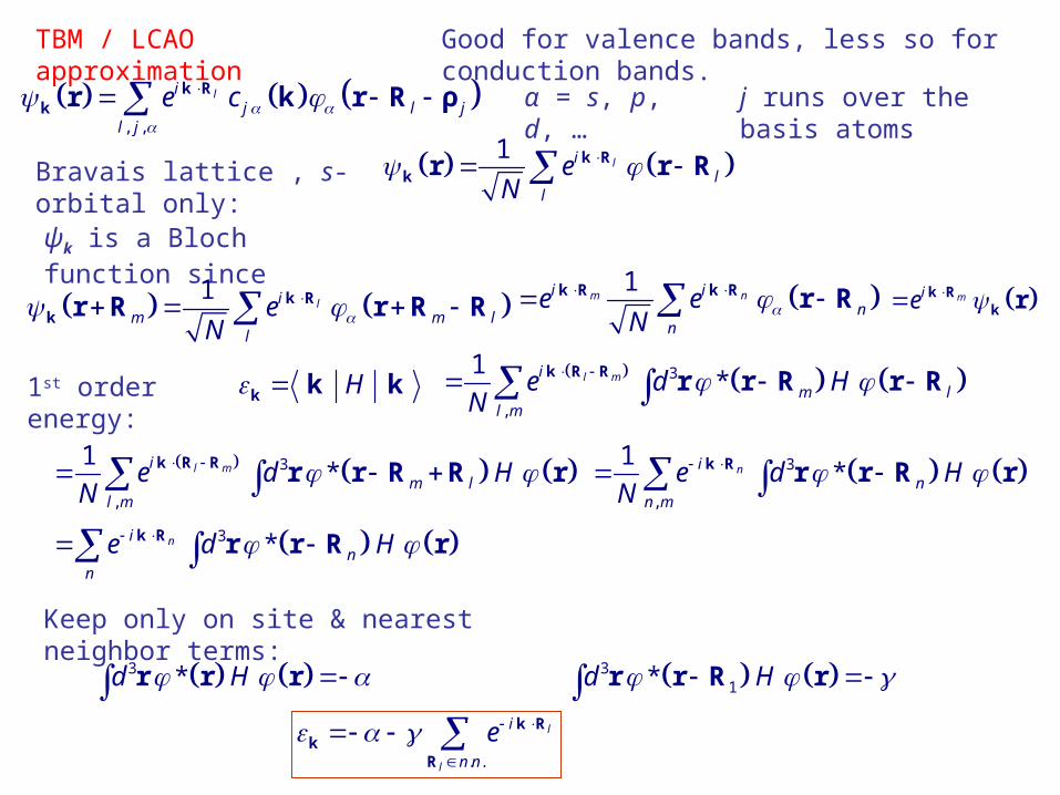
TBM / LCAO approximation Good for valence bands, less so for conduction bands.
, ,
lij l j
l j
e c
k Rk r k r R ρ α = s, p, d, …
ψk is a Bloch function since
j runs over the basis atoms
1li
m m ll
eN
k Rk r R r R R 1
m ni in
n
e eN
k R k R r R mie k R
k r
1st order energy: H k k k 3
,
1*l mi
m ll m
e d HN
k R R r r R r R
Bravais lattice , s-orbital only: 1li
ll
eN
k Rk r r R
3
,
1*l mi
m ll m
e d HN
k R R r r R R r 3
,
1*ni
nn m
e d HN
k R r r R r
3 *nin
n
e d H k R r r R r
Keep only on site & nearest neighbor terms:
3 *d H r r r 31*d H r r R r
. .
l
l
i
n n
e
k Rk
R
0/
0
2 1 aRy ea
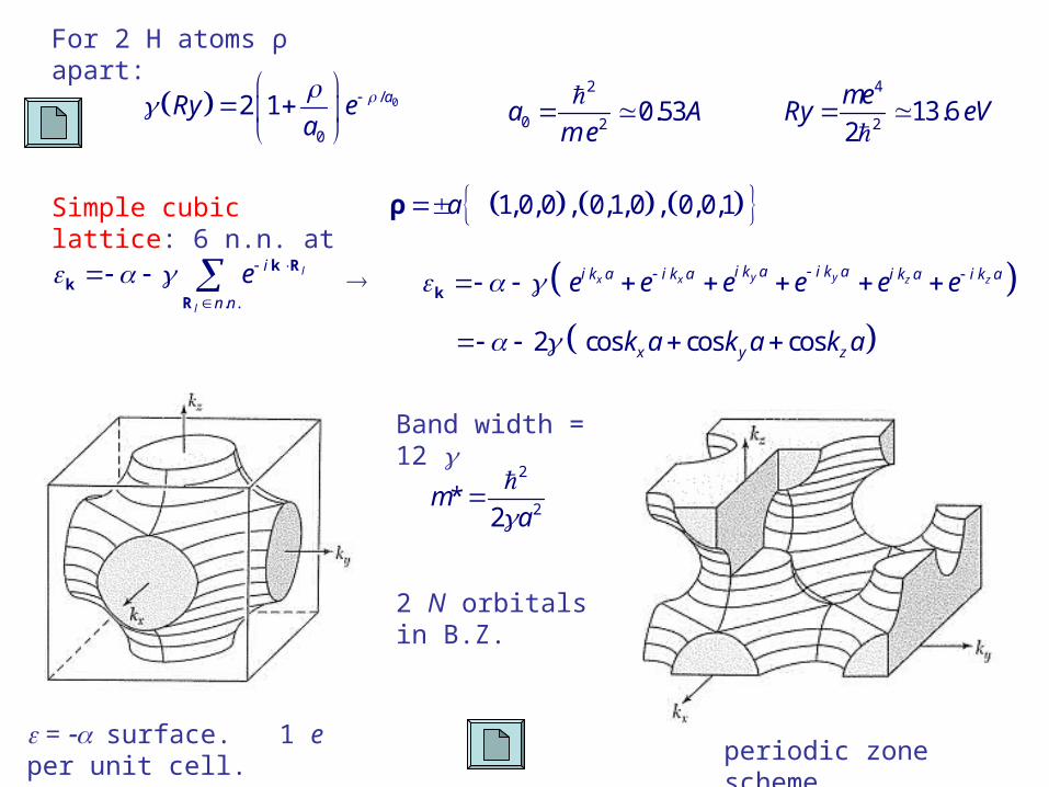
For 2 H atoms ρ apart:
2
0 20.53a A
m e
4
213.6
2
meRy eV
Simple cubic lattice: 6 n.n. at
1,0,0 , 0,1,0 , 0,0,1aρ
y yx x z zi k a i k ai k a i k a i k a i k ae e e e e e k
2 cos cos cosx y zk a k a k a
Band width = 12
= surface. 1 e per unit cell.periodic zone scheme
2
2*
2m
a
2 N orbitals in B.Z.
. .
l
l
i
n n
e
k Rk
R
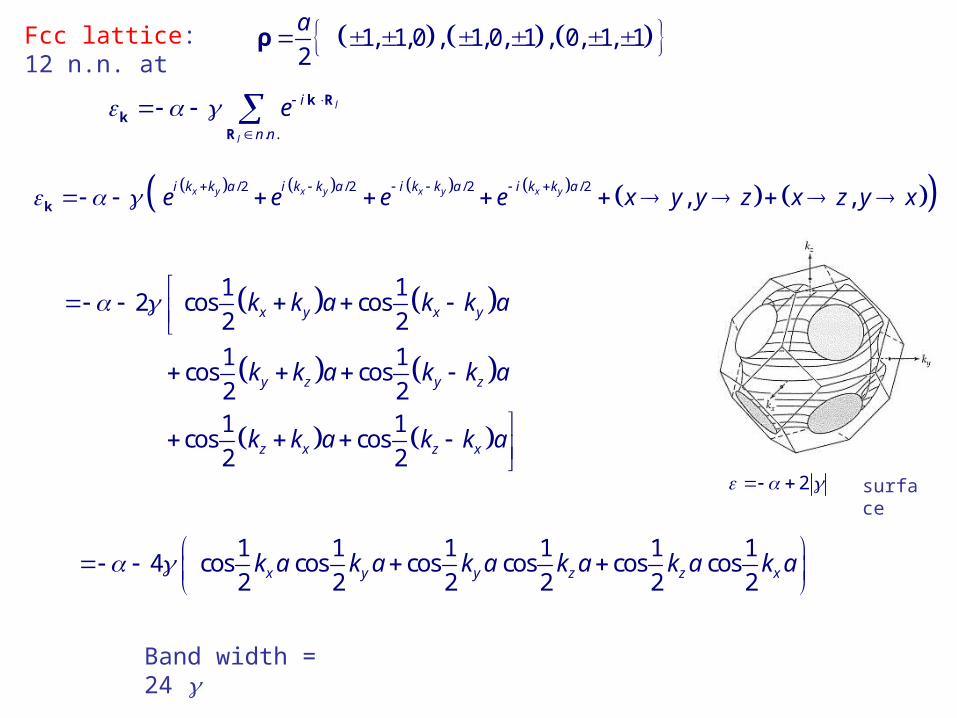
Fcc lattice: 12 n.n. at 1, 1,0 , 1,0, 1 , 0, 1, 12
a ρ
/2 /2 /2 /2, ,x y x y x y x yi k k a i k k a i k k a i k k a
e e e e x y y z x z y x k
1 12 cos cos
2 2
1 1cos cos
2 21 1
cos cos2 2
x y x y
y z y z
z x z x
k k a k k a
k k a k k a
k k a k k a
Band width = 24
1 1 1 1 1 14 cos cos cos cos cos cos
2 2 2 2 2 2x y y z z xk a k a k a k a k a k a
2 surface
. .
l
l
i
n n
e
k Rk
R
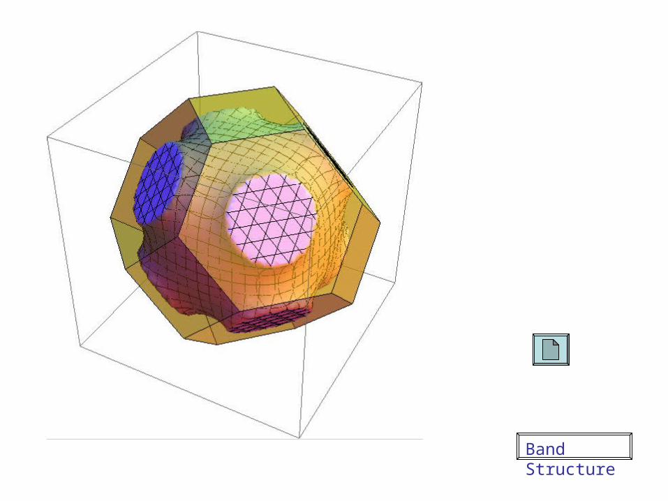
Band Structure
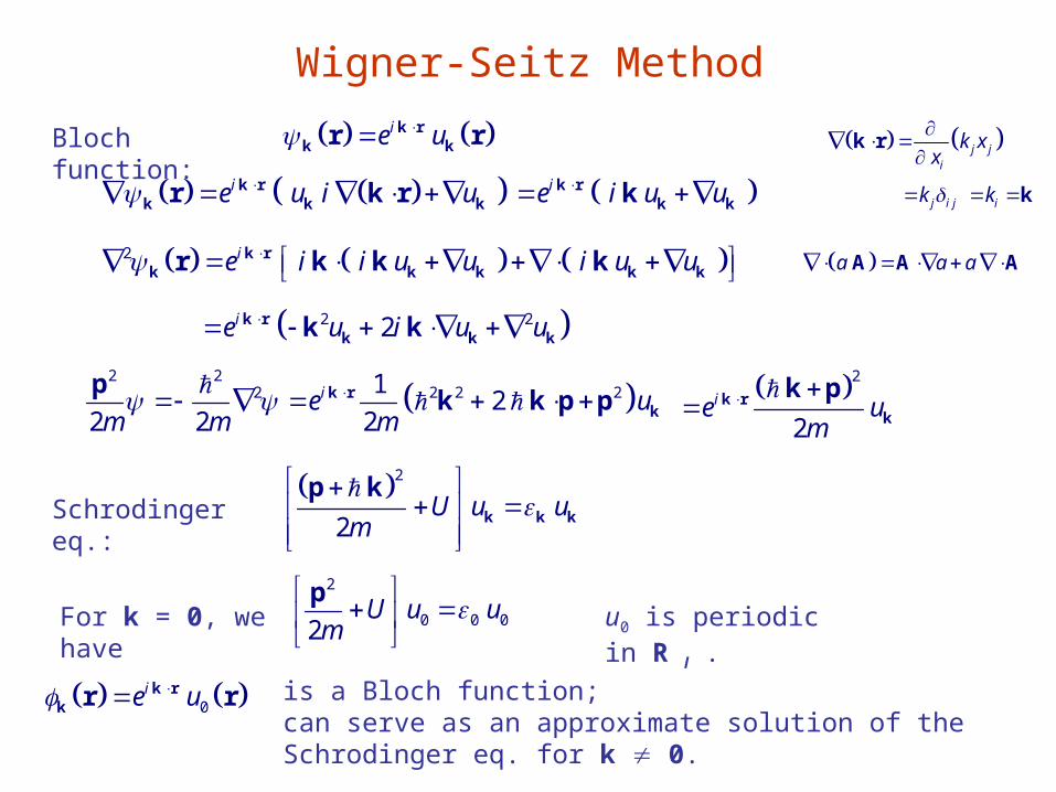
Wigner-Seitz Method
Bloch function: ie u kk
rk r r
Schrodinger eq.:
ie u i u kk k k
rr k r
2 ie i i u u i u u k
k k k k krr k k k
2 22ie u i u u kk k k
r k k
22 2
22 212
2 2 2ie u
m m m rk
k
pk pk p
2
2ie u
m
kk
r k p
2
2U u u
m
k k k
p k
a a a A A A
j ji
k xx
k r
j i jk ik k ie i u u kk k
r k
For k = 0, we have2
0 0 02U u u
m
pu0 is periodic in R l .
is a Bloch function;can serve as an approximate solution of the Schrodinger eq. for k 0.
0ie u k r
k r r
0ie u k r
k r r 0 0 0H u u
2 2
0 0 02H u u
m m k k
kk p
202
iH e U um
krk p k
r 2
0
2
0ie u
m m
rk kpk
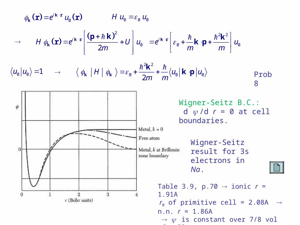
0 0 1u u Prob 8
Wigner-Seitz result for 3s electrons in Na.
Wigner-Seitz B.C.: d /d r = 0 at cell boundaries.
Table 3.9, p.70 ionic r = 1.91A r0 of primitive cell = 2.08A n.n. r = 1.86A is constant over 7/8 vol of cell.
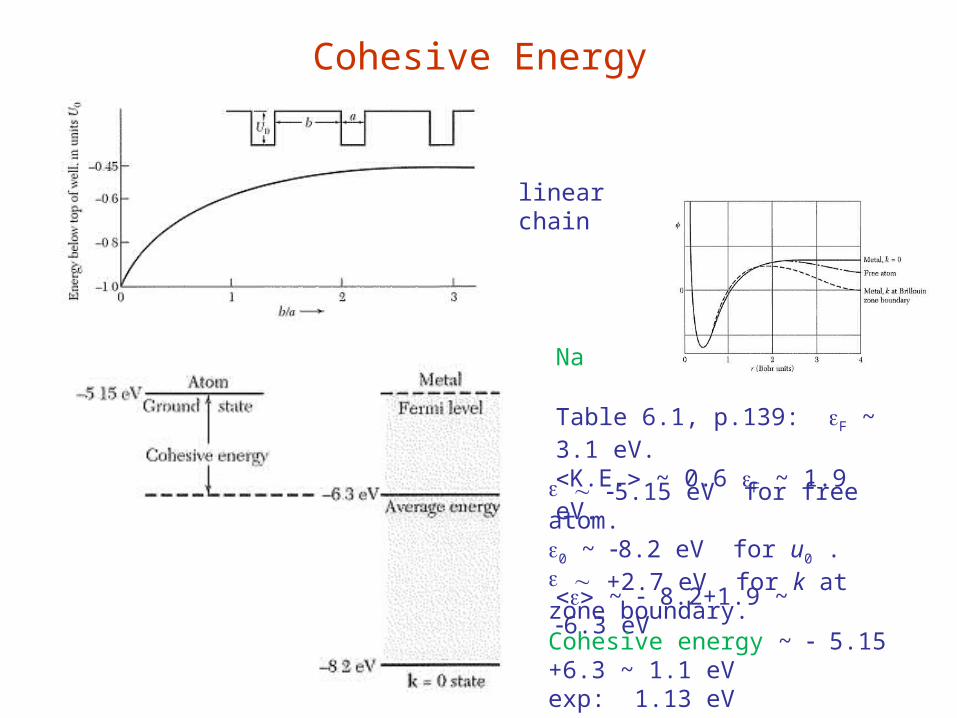
Cohesive Energy
linear chain
Na
5.15 eV for free atom.0 ~ 8.2 eV for u0 . +2.7 eV for k at zone boundary.
Table 6.1, p.139: F ~ 3.1 eV.K.E. ~ 0.6 F ~ 1.9 eV.
~ 8.2+1.9 ~ 6.3 eV
Cohesive energy ~ 5.15 +6.3 ~ 1.1 eVexp: 1.13 eV
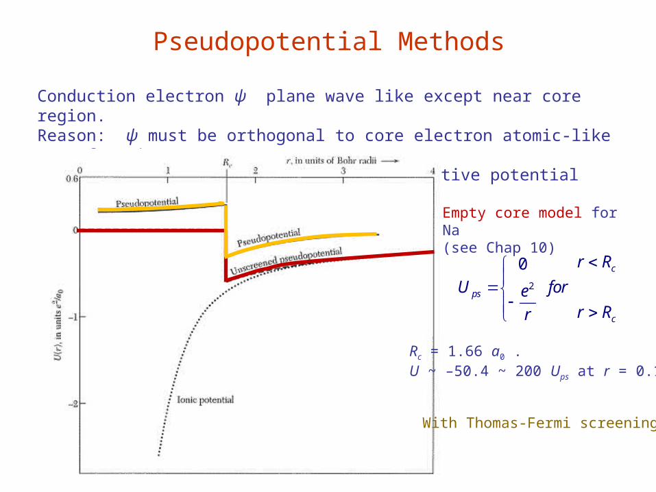
Pseudopotential Methods
Conduction electron ψ plane wave like except near core region.Reason: ψ must be orthogonal to core electron atomic-like wave functions.Pseudopotential: replace core with effective potential that gives true ψ outside core.
Empty core model for Na(see Chap 10)
Rc = 1.66 a0 .U ~ –50.4 ~ 200 Ups at r = 0.15
2
0 c
ps
c
r R
U forer Rr
With Thomas-Fermi screening.
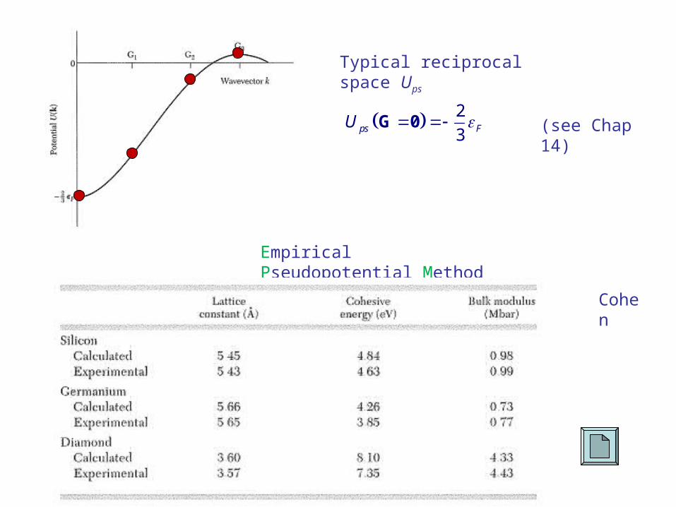
Typical reciprocal space Ups
Empirical Pseudopotential Method
Cohen
2
3ps FU G 0 (see Chap 14)
Experimental Methods in Fermi Surface Studies
• Quantization of Orbits in a Magnetic Field
• De Haas-van Alphen Effect
• Extremal Orbits
• Fermi Surface of Copper
• Example: Fermi Surface of Gold
• Magnetic Breakdown

Experimental methods for determining Fermi surfaces:• Magnetoresistance• Anomalous skin effect• Cyclotron resonance• Magneto-acoustic geometric effects• Shubnikov-de Haas effect• de Haas-van Alphen effect
Experimental methods for determining momentum distributions:• Positron annihilation• Compton scattering• Kohn effect
Metal in uniform B field → 1/B periodicity
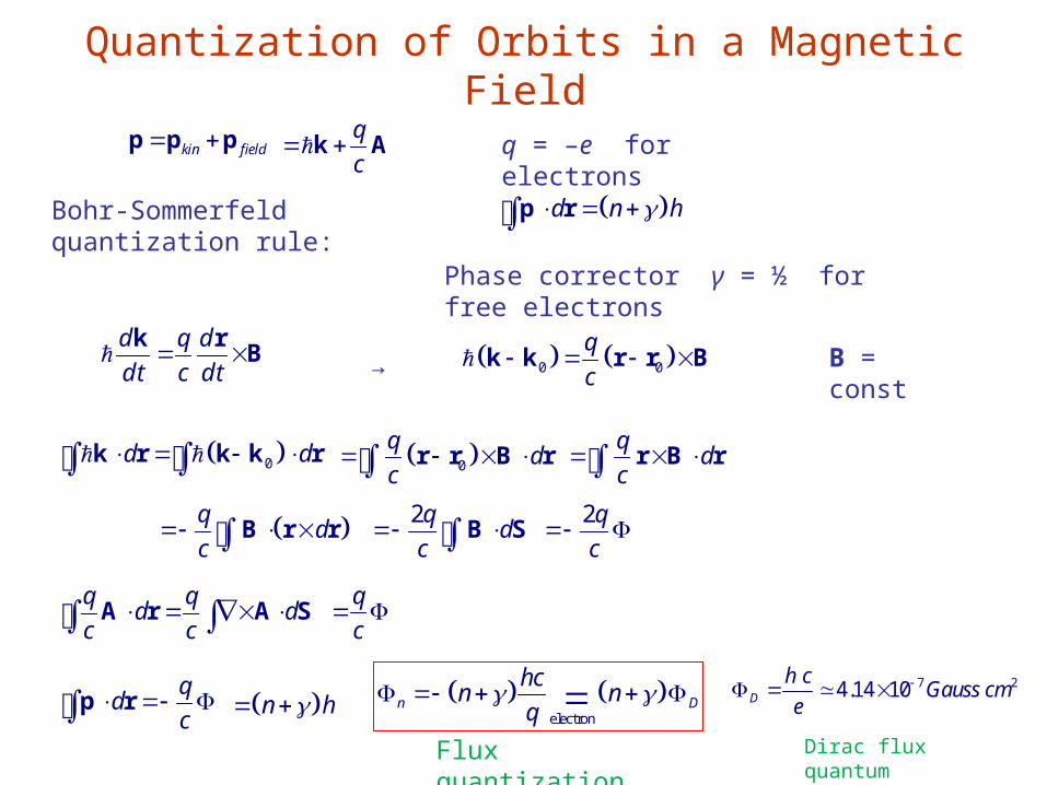
Quantization of Orbits in a Magnetic Field
kin field p p p q
c k A
Bohr-Sommerfeld quantization rule: d n h p r
Phase corrector γ = ½ for free electrons
q = –e for electrons
d q d
dt c dt
k rB → 0 0
q
c k k r r B B = const
0d d k r k k r qd
c r B r
qd
c B r r
2qd
c B S
2q
c
0
qd
c r r B r
q qd d
c c A r A S
q
c
qd
c p r n h
electronn D
hcn n
q 7 24.14 10D
h cGauss cm
e
Flux quantization Dirac flux quantum
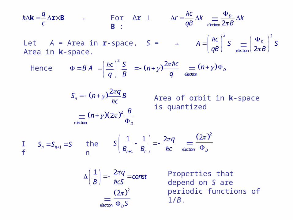
q
c k r B →
cr k
qB
For Δr B :
Let A = Area in r-space, S = Area in k-space. →2
cA S
qB
Hence2
c S
q B
B A 2 cn
q
2n
qS n B
c
Area of orbit in k-space is quantized
1
1 1 2
n n
qS
B B c
If 1n nS S S then
1 2 qconst
B cS
Properties that depend on S are periodic functions of 1/B.
2electron
2D
Bn
2
electron
2
D
electron
Dn
2
electron
2
DS
2
electron 2D SB
electron 2D kB
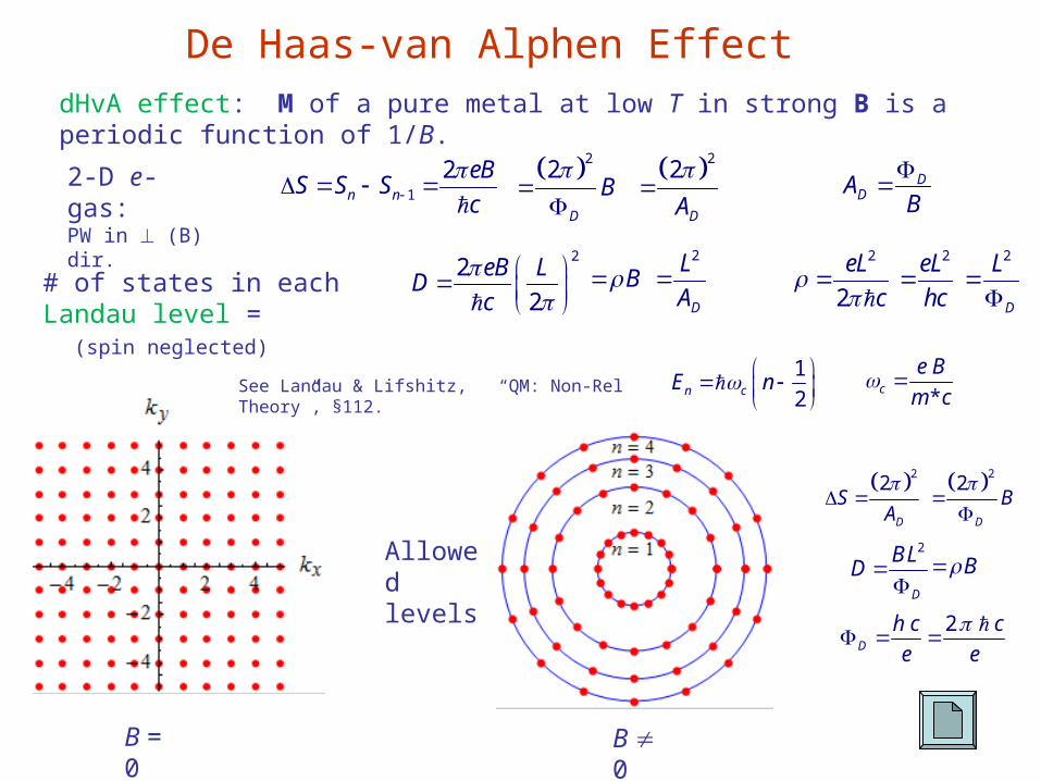
De Haas-van Alphen Effect dHvA effect: M of a pure metal at low T in strong B is a periodic function of 1/B.
1
2n n
eBS S S
c
2-D e-gas:PW in (B) dir.
# of states in each Landau level = (spin neglected)
22
2
eB LD
c
B2
2
eL
c
22
D
B
22
DA
2eL
hc
2
D
L
2
D
L
A
DDA
B
B = 0
Allowed levels
22
D
SA
2
D
BLD
22
D
B
B
2D
h c c
e e
1
2n cE n
*c
e B
m c See Landau & Lifshitz, “QM: Non-Rel Theory”, §112.
B 0

10T TE E B 2 30T T TE B E E B
1 2 3B B B
1
2n cE n
*c
e B
m c
For the sake of clarity, n of the occupied states in the circle diagrams is 1 less than that in the level diagrams.
Number of e = 48
D = 16 D = 19 D = 24
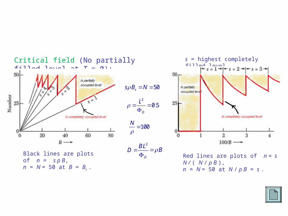
Critical field (No partially filled level at T = 0):
50ss B N
s = highest completely filled level
2
0.5D
L
2
D
BLD
B
Black lines are plots of n = s ρ B,n = N = 50 at B = Bs .
Red lines are plots of n = s N / ( N / ρ B ),n = N = 50 at N / ρ B = s .
100N
1
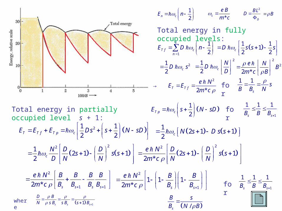
2n cE n
*c
e B
m c
1
1
2
s
T f cn
E D n
2
D
BLD
B
1 11
2 2cD s s s
Total energy in fully occupied levels:
21
2 cD s
Total energy in partially occupied level s + 1: 1
2T p cE s N sD
21 1
2 2T T f T p cE E E Ds s N sD 1
2 1 12 c N s D s s
21
2 c
ND
D
→2
2 *T T f
e NE E
m c
for1 1
s
sB B N
for
2
2
2 *
e NB
m c B
221
2 1 12 c
N D Ds s s
D N N
22
2 1 12 *
e N D Ds s s
m c N N
2
1 12 * s s s s
e N B B B B
m c B B B B
2
1
1 1 12 * s s
e N B B
m c B B
for
1
1 1 1
s sB B B
1
1 1 1
s sB B B
11s s s
D B
N s B s B s B
where
/s
B s
B N B
TE
B
2
1
1 1
2 *ss s
e NB
m c B B
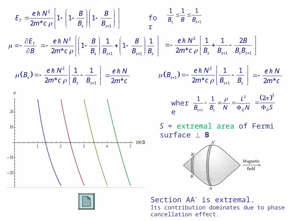
2
1
1 1 12 *T
s s
e N B BE
m c B B
for
1
1 1 1
s sB B B
2
1 1
1 11 1
2 * s s s s
e N B B
m c B B B B
2
1 1
1 1 2
2 * s s s s
e N B
m c B B B B
2 *
e N
m c
2
11
1 1
2 *ss s
e NB
m c B B
2 *
e N
m c
2
1
1 1
s s D
L
B B N N
where 22
DS
S = extremal area of Fermi surface B
Section AA is extremal.Its contribution dominates due to phase cancellation effect.
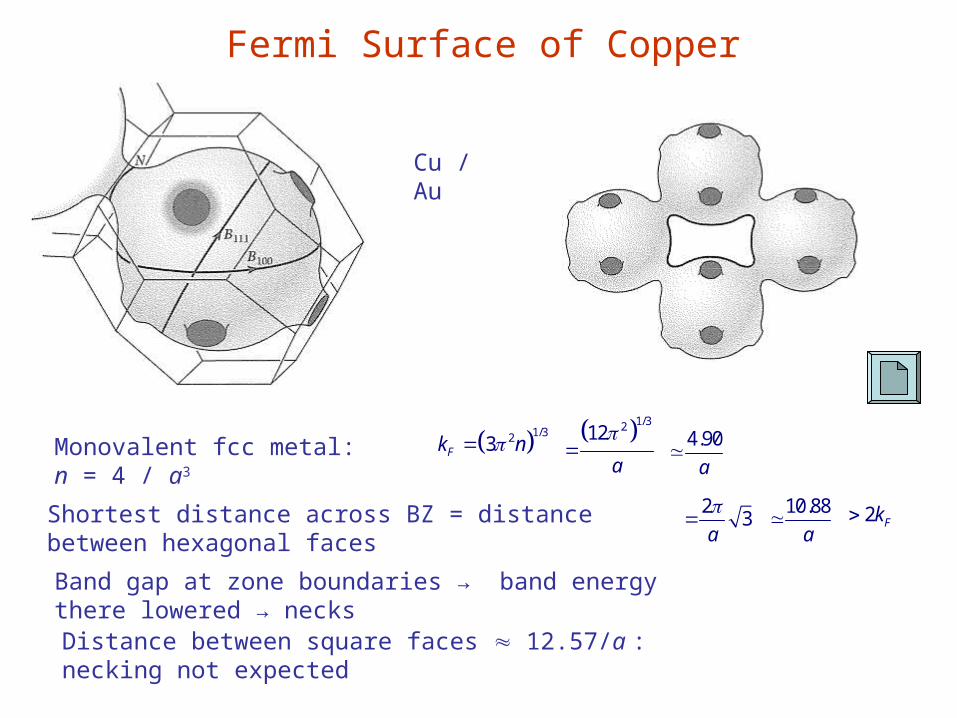
Fermi Surface of Copper
Cu / Au
Monovalent fcc metal: n = 4 / a3 1/323Fk n 1/3212
a
4.90
a
Shortest distance across BZ = distance between hexagonal faces 23
a
2 Fk10.88
a
Band gap at zone boundaries → band energy there lowered → necks
Distance between square faces 12.57/a : necking not expected
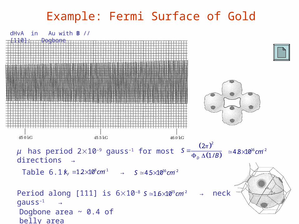
Example: Fermi Surface of GolddHvA in Au with B // [110]: Dogbone
μ has period 210–9 gauss–1 for most directions →
22
1/D
SB
16 24.8 10 cm
Table 6.1: 8 11.2 10Fk cm → 16 24.5 10S cm
Period along [111] is 610–8 gauss–1 → 15 21.6 10S cm → neck
Dogbone area ~ 0.4 of belly area
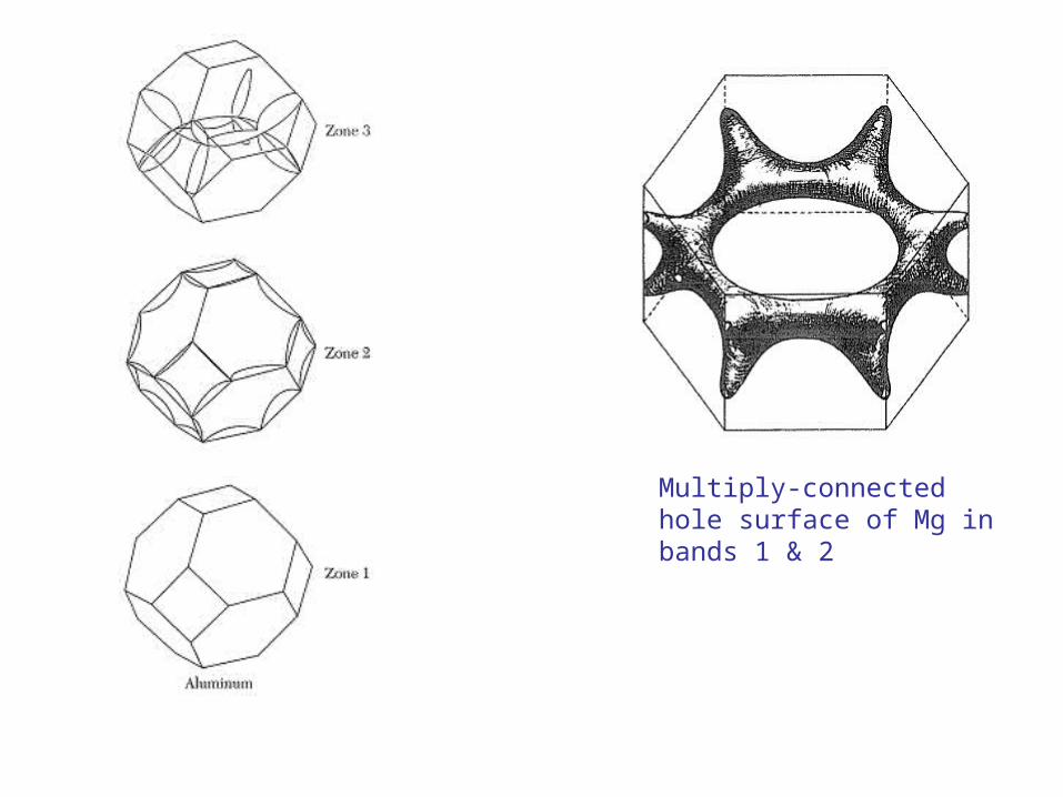
Multiply-connected hole surface of Mg in bands 1 & 2
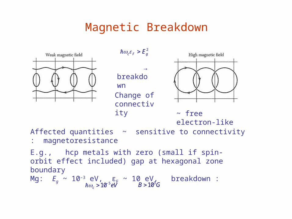
Magnetic Breakdown
~ free electron-like
→breakdown
Change of connectivity
Affected quantities ~ sensitive to connectivity : magnetoresistance
2c F gE
E.g., hcp metals with zero (small if spin-orbit effect included) gap at hexagonal zone boundaryMg: Eg ~ 10–3 eV, εF ~ 10 eV, breakdown :
510c eV 310B G


![Homogeneous manifolds whose geodesics are orbits. · Homogeneous manifolds whose geodesics are orbits 7 are g.o. spaces. In [42] O. Kowalski, F. Prufer and L. Vanhecke gave an explicit](https://static.fdocument.org/doc/165x107/5edc86e5ad6a402d66673922/homogeneous-manifolds-whose-geodesics-are-homogeneous-manifolds-whose-geodesics.jpg)