ALPHA-THEORY: AN ELEMENTARY AXIOMATICS FORdinasso/papers/14.pdf · ALPHA-THEORY: AN ELEMENTARY...
32
ALPHA-THEORY: AN ELEMENTARY AXIOMATICS FOR NONSTANDARD ANALYSIS VIERI BENCI AND MAURO DI NASSO Abstract. The methods of nonstandard analysis are presented in elementary terms by postulating a few natural properties for an infinite “ideal” number α. The resulting axiomatic system, including a formalization of an interpretation of Cauchy’s idea of infinitesimals, is related to the existence of ultrafilters with special properties, and is independent of ZFC. The Alpha-Theory supports the feeling that technical notions such as superstructure, ultrapower and the transfer principle are definitely not needed in order to carry out calculus with actual infinitesimals. Introduction In early stages of calculus, up to the first years of the nineteenth century, infinitesimal quantities were widely used to develop many of the classic results of analysis. Afterwards, at the end of nineteenth century, a severe foundational criticism led to the current ²-δ formalization due to Weierstrass, and infinitesimal and infinite numbers were banned from calculus. Nonstandard analysis was introduced by A. Robinson [44, 45] in the early sixties. By using the machinery of model theory, a branch of mathematical logic, he succeeded in providing the actual use of infinitesimal numbers with rigorous foundations, thus giving a solution to a century-old problem. Since then, the methods of nonstandard analysis have been successfully applied and have led to new results in such diverse fields of mathe- matics as functional analysis, measure and probability theorons, additive number theory, stochastic analysis, hydromechanics, etc. (See [1] for a broad collection of reviews. See also [34] for nonstandard methods applied to additive number theory.) Unfortunately, very soon the formalism of Robinson’s original presentation appeared too technical to many, and not directly usable by those mathematicians without a good background in logic. Over the last forty years, many attempts have been made in order to simplify the foundational matters and popularize nonstandard analysis by means of “easy to grasp” presentations. Most notably, the pioneering work by W.A.J. Luxemburg [40], where a direct use of ultrapowers was made; the superstructure approach [46] presented by A. Robinson jointly with E. Zakon within a set-theoretic framework; the elementary axiomatics [35] given by H.J. Keisler in the seventies (the relative textbook [36] was actually adopted for calculus classes with good results in several countries); the algebraic presentation of hyperreals by W.S. Hatcher [29], then extended by the authors to the full generality of nonstandard analysis [4, 5]; and finally the recent “gentle” introduction by W. Henson [31]. 2000 Mathematics Subject Classification. 26E35 Nonstandard analysis; 03E65 Other hypotheses and axioms; 03C20 Ultraproducts and related constructions. 1
Transcript of ALPHA-THEORY: AN ELEMENTARY AXIOMATICS FORdinasso/papers/14.pdf · ALPHA-THEORY: AN ELEMENTARY...
ALPHA-THEORY: AN ELEMENTARY AXIOMATICS FORNONSTANDARD ANALYSIS
VIERI BENCI AND MAURO DI NASSO
Abstract. The methods of nonstandard analysis are presented in elementary termsby postulating a few natural properties for an infinite “ideal” number α. The resultingaxiomatic system, including a formalization of an interpretation of Cauchy’s idea ofinfinitesimals, is related to the existence of ultrafilters with special properties, and isindependent of ZFC. The Alpha-Theory supports the feeling that technical notions suchas superstructure, ultrapower and the transfer principle are definitely not needed in orderto carry out calculus with actual infinitesimals.
Introduction
In early stages of calculus, up to the first years of the nineteenth century, infinitesimalquantities were widely used to develop many of the classic results of analysis. Afterwards,at the end of nineteenth century, a severe foundational criticism led to the current ε-δformalization due to Weierstrass, and infinitesimal and infinite numbers were banned fromcalculus.
Nonstandard analysis was introduced by A. Robinson [44, 45] in the early sixties. Byusing the machinery of model theory, a branch of mathematical logic, he succeeded inproviding the actual use of infinitesimal numbers with rigorous foundations, thus givinga solution to a century-old problem. Since then, the methods of nonstandard analysishave been successfully applied and have led to new results in such diverse fields of mathe-matics as functional analysis, measure and probability theorons, additive number theory,stochastic analysis, hydromechanics, etc. (See [1] for a broad collection of reviews. Seealso [34] for nonstandard methods applied to additive number theory.)
Unfortunately, very soon the formalism of Robinson’s original presentation appearedtoo technical to many, and not directly usable by those mathematicians without a goodbackground in logic. Over the last forty years, many attempts have been made in order tosimplify the foundational matters and popularize nonstandard analysis by means of “easyto grasp” presentations. Most notably, the pioneering work by W.A.J. Luxemburg [40],where a direct use of ultrapowers was made; the superstructure approach [46] presentedby A. Robinson jointly with E. Zakon within a set-theoretic framework; the elementaryaxiomatics [35] given by H.J. Keisler in the seventies (the relative textbook [36] wasactually adopted for calculus classes with good results in several countries); the algebraicpresentation of hyperreals by W.S. Hatcher [29], then extended by the authors to the fullgenerality of nonstandard analysis [4, 5]; and finally the recent “gentle” introduction byW. Henson [31].
2000 Mathematics Subject Classification. 26E35 Nonstandard analysis; 03E65 Other hypotheses andaxioms; 03C20 Ultraproducts and related constructions.
1
2 VIERI BENCI AND MAURO DI NASSO
Currently, most practitioners work in the setting of the superstructure approach orfollow Nelson’s Internal Set Theory IST [42]. In this paper, we present a new alterna-tive approach to nonstandard analysis aimed at showing that technical notions such assuperstructure, ultrafilter, ultrapower, bounded formula and the transfer principle, arenot needed to rigorously develop calculus with infinitesimals. We proceed axiomatically.Precisely, the Alpha-Theory consists of a few natural properties postulated for an “ideal”natural number α, to be thought as “infinitely large”.
Historically, the idea of adjoining a new number that, in some precise sense, behaveslike a very large natural number, goes back to the pre-Robinsonian work by C. Schmiedenand D. Laugwitz [48]. They considered a new symbol Ω and postulated that if a given“formula” is true for all sufficiently large natural numbers, then the “formula” is truefor Ω as well. The resulting theory has a constructive flavour, and it inspired various“non-classical” presentations of nonstandard analysis.1
Although well suited to provide a foundational justification for the use of infinitesimalsand to develop large parts of calculus (see [39]), the Ω-approach soon revealed inadequatefor applications in classical mathematics. Most notably, the crucial drawback is that thenonstandard reals contain zero divisors and are only a partially ordered ring.
In a few years, with the turn of the sixties, that approach was superseded by themore powerful “Robinsonian” analysis. However, it seems correct to say that the Ω-approach was a turning point in the treatment of the idea of infinitesimals. Even if therewas no direct influence on nonstandard analysis as practiced today, we think it was notby chance that in the seminal paper [44], Robinson himself acknowledged the work bySchmieden and Laugwitz as a “recent and rather successful effort of developing a calculusof infinitesimals”.
In some sense, the Alpha-Theory can be seen as a convenient strengthening of theΩ-approach. On the one hand, it preserves the intuitive appeal of postulating a few el-ementary properties which are preserved by N-sequences when extended to the “ideal”point at infinity; on the other hand, has the full strength of Robinsonian nonstandardanalysis. Besides, the Alpha-Theory seems to be the right framework to formalize anidea of an infinitesimal number which has some philosophical and historical relevance.According to J. Cleave [16, 17], Cauchy’s conception of infinitesimals can be described as“values of null real sequences at infinity”. Now, the very idea of values of sequences atinfinity is what the Alpha-Theory is aimed to formalize. The Cauchy’s infinitesimals prin-ciple, stating that every infinitesimal number is the value at infinity of some infinitesimalsequence, is naturally formulated in our context. We shall also consider the stronger ver-sion postulating that every nonzero infinitesimal is the value at infinity of some monotonesequence.
As for the foundational matters, the Alpha-Theory without Cauchy’s principles admitsa faithful interpretation in Zermelo-Fraenkel Set Theory ZFC. Thus, informally we cansay that any theorem in “ordinary mathematics” which is proved by the Alpha-Theory istrue.
Inspired by the criticism by N. Cutland, C. Kessler, E. Kopp and D. Ross [19] on themathematical content of the Cleave’s interpretation mentioned above, we also investigate
1See e.g. the overview [43] by E. Palmgren. A recent non-nonstandard treatment of calculus waspresented by J.M. Henle [30]. Interesting articles on the constructive viewpoint on nonstandard analysiscan be found in the recent book [49].
ALPHA-THEORY 3
the foundational strength of Cauchy’s infinitesimals principles and prove the following re-sults: The Alpha-Theory plus Cauchy’s principle is equiconsistent with ZFC plus “thereexists a P-point”, and the Alpha-Theory plus the strong Cauchy’s principle is equicon-sistent with ZFC plus “there exists a selective ultrafilter” (we recall that the existence ofeither a P -point or a selective ultrafilter is independent of ZFC). Informally, this meanson the one hand that Cauchy’s principles are “sound” (i.e. they do not bring contra-dictions), on the other hand they allow proving theorems that “ordinary mathematics”cannot prove. (Clearly, the blanket assumption is the consistency of ZFC).
In this paper, we focused on the elementary nature of our approach, and in one Ap-pendix we also included a small number of basic examples taken from calculus, so to givea taste of nonstandard methods “in action”. All the technical parts are relegated to thelast Section, which contains a formal presentation of the Alpha-Theory as a first-ordertheory, and the consistency proofs.
Some additional comments for “nonbeginners”.The Alpha-Theory has the full strength of Robinsonian nonstandard analysis with count-able saturation. In fact, both the transfer principle for all bounded formulas and thecountable saturation property are theorems of the Alpha-Theory. According to the popu-lar plan of this paper, in the exposition, as well as in the Appendix ”A Little Calculus”,the transfer principle is never mentioned. Rather, on a case to case basis, we prove directlyonly those instances that are actually needed to obtain the desired results.
Also from a foundational point of view, the Alpha-Theory is aimed to simplify mat-ters. In the superstructure approach, two different universes are considered, namely thestandard model and the nonstandard model. In our context there is a single universe, the“usual” world of mathematics where all axioms of ZFC except foundation are assumed.Moreover, contrarily to IST and other nonstandard set theories that have been presentedin the literature (see [21] for a survey), external sets are available without restrictions, andthe nonstandard embedding ∗ is defined for all sets. As a consequence, ∗ can be iteratedto get things like the hyper-hyperreal numbers (R∗)∗, or the star-transforms of externalobjects, such as Loeb measures, etc. (E.g., the double nonstandard iterations used byV.A. Molchanov [41] to study compactifications in topology, can be naturally formalizedin the framework of the Alpha-Theory.)
Acknowledgements
The authors thank Marco Forti for valuable discussions, and thank Jerry Keisler for useful remarks ona previous version of the paper.
1. The Alpha-Theory.
Our approach is based on the existence of a new mathematical object, namely α. Wecan think of α as a new ideal natural number added to N, in a similar way as the imaginaryunit i can be seen as a new ideal number added to the real numbers. By adopting thenotion of numerosity introduced in [6], an interpretation of the ideal number α can begiven as the numerosity of the set of natural numbers (see [7]). However, in order to helpthe intuition, it is enough to think of α as a “very large” natural number.
4 VIERI BENCI AND MAURO DI NASSO
Before going into the axioms, we remark that the blanket assumption is that all usualprinciples of “ordinary mathematics” are assumed. Informally, we can say that by adopt-ing our theory, one can construct sets and functions according to the “usual” practice ofmathematics, with no restrictions whatsoever.2
1.1. The five axioms.According to the usual foundational framework of mathematics, namely Zermelo-Fraenkelset theory ZFC, every object of the mathematical universe is a set. Clearly, the philo-sophical plausibility of such an assumption is highly disputable, but the foundationalsuccess of pure set theory is due to the fact that virtually all entities of mathematics canactually be coded as sets. For instance, an ordered pair 〈a, b〉 can be identified with theKuratowski pair k = a , a, b (so that the two elements a, b are obtained as elementsof elements of k, the first element of the ordered pair being the one that belongs to bothelements of k); an equivalence relation ∼ can be identified with the set of ordered pairs〈a, b〉 | a ∼ b that satisfy it; a function f : A → B can be identified with its graphΓ(f) = 〈a, b〉 | f(a) = b, etc. As for numbers, one can consider the von Neumann nat-ural numbers : 0 = ∅, n + 1 = n ∪ n (so that each natural number is the set of itspredecessors and the order relation is given by the membership). One can define the inte-gers (and the rationals) as ordered pairs of naturals (of integers, resp.) identified modulosuitable equivalence relations. One can then define the real numbers as equivalence classesof Cauchy sequences, the complex numbers as a quotient of ordered pairs of reals, etc.
However, in practice it is often convenient to have atoms available, i.e. primitive objectswhich are not sets. For instance, it is more natural to many mathematicians to think ofnumbers as individuals rather than sets. So, to simplify matters, in the following weassume a set of atoms A, which includes all real numbers R ⊂ A. When talking aboutsets we shall always mean nonatoms, i.e. objects that are identified with the collectionof their elements. In particular, there can be only one set with no elements, namelythe empty set ∅. When talking about elements or entities, we shall mean objects of theuniverse in general, i.e. either atoms or sets.3 In the sequel, by sequence we shall alwaysmean a function whose domain is the set of natural numbers.
The use of α is governed by the following five axioms.
α1. Extension Axiom.For every sequence ϕ there is a unique element ϕ[α], called the “ideal value of ϕ” or the“value of ϕ at infinity”.
The next axiom gives a natural coherence property with respect to compositions.
α2. Composition Axiom.If ϕ and ψ are sequences and if f is any function such that compositions f ϕ and f ψmake sense, then
ϕ[α] = ψ[α] ⇒ (f ϕ)[α] = (f ψ)[α]
So, if two sequences takes the same value at infinity, by composing them with any givenfunction, we again obtain sequences with the same value at infinity.
2A formalization of what we mean by “usual principles of mathematics” (i.e. our underlying set theory)is given in the last Section 6 where we concentrate on the technical and foundational matters.
3We remark that our theory can also be formulated in a purely set theoretic context (i.e. where noatoms exist). See [24].
ALPHA-THEORY 5
α3. Number Axiom.If cr : n 7→ r is the constant sequence with value r ∈ R, then cr[α] = r. If 1N : n 7→ n isthe identity sequence on N, then 1N[α] = α /∈ N.
The first part of this axiom simply says that those sequences which constantly equal areal number, have the expected ideal values. The latter condition says that α is obtainedas the value at infinity of the identity sequence, and that α is actually a new number.Notice that 1N provides a first example of a sequence ϕ : N→ A such that ϕ[α] /∈ A.
The next axiom supplies other examples of sequences which have the “expected” idealvalues.
α4. Pair Axiom.For all sequences ϕ, ψ and ϑ:
ϑ(n) = ϕ(n), ψ(n) for all n ⇒ ϑ[α] = ϕ[α], ψ[α]The next (and last) axiom says what elements are there in ideal values.
α5. Internal Set Axiom.If ψ is a sequence of atoms, then ψ[α] is an atom. If c∅ : n 7→ ∅ is the sequence withconstant value the empty set, then c∅[α] = ∅. If ψ is a sequence of nonempty sets, then
ψ[α] = ϕ[α] | ϕ(n) ∈ ψ(n) for all nThe name Internal Set Axiom is justified because our values at infinity ψ[α] correspond
to the internal sets in the usual terminology of nonstandard analysis (see Section 4.1).As an immediate consequence of this axiom, the membership relation is preserved at
the ideal values. That is, if ϕ(n) ∈ ψ(n) for all n, then ϕ[α] ∈ ψ[α]. Besides, when ψ asequence of nonempty sets, all elements of ψ[α] are obtained in this way. That is, theyall are values at infinity of sequences which are pointwise members of ψ.
An interesting example is the following. Suppose ϕ is a two-valued sequence, sayϕ : N → −1, 1. Then its ideal value makes no surprise, i.e. either ϕ[α] = −1 orϕ[α] = 1 (but in general it cannot be decided which is the case). This fact directly followsfrom the pair axiom and the internal set axiom.
Although well-suited for the “working” mathematician, we remark that the above fiveaxioms are only given in a “semi-formal” fashion. Indications for a rigorous formalizationas sentences of a suitable first-order language are given in Section 6.
1.2. First consequences of the axioms.In this subsection, we list a collection of basic and natural properties of the values atinfinity, which directly follow from the axioms. In order to make the exposition as smoothas possible and go quickly to more interesting topics, we shall postpone the proofs toAppendix B.
Let ξ and ζ be two sequences. In the following, for the sake of simplicity we shall writeξ(n) = ζ(n) to mean that such an equality holds for all n ∈ N. Similarly, we shall writeξ(n) 6= ζ(n), ξ(n) ∈ ζ(n), ξ(n) ⊆ ζ(n) etc., to mean that those relationships hold for alln.
The first Proposition shows that all basic set operations (except the powerset) arepreserved at infinity.
6 VIERI BENCI AND MAURO DI NASSO
Proposition 1.1. Assume that ϕ, ψ are sequences of nonempty sets.4 Then the followinghold:
(1) Difference: ϕ(n) 6= ψ(n) ⇒ ϕ[α] 6= ψ[α] and ϕ(n) /∈ ψ(n) ⇒ ϕ[α] /∈ ψ[α];(2) Subset: ϕ(n) ⊆ ψ(n) ⇒ ϕ[α] ⊆ ψ[α];(3) Union: ϑ(n) = ϕ(n) ∪ ψ(n) ⇒ ϑ[α] = ϕ[α] ∪ ψ[α];(4) Intersection: ϑ(n) = ϕ(n) ∩ ψ(n) ⇒ ϑ[α] = ϕ[α] ∩ ψ[α];(5) Setminus: ϑ(n) = ϕ(n) \ ψ(n) ⇒ ϑ[α] = ϕ[α] \ ψ[α];(6) Ordered pair: ϑ(n) = 〈ϕ(n), ψ(n)〉 ⇒ ϑ[α] = 〈ϕ[α], ψ[α]〉;(7) Cartesian product: ϑ(n) = ϕ(n)× ψ(n) ⇒ ϑ[α] = ϕ[α]× ψ[α].
Clearly, properties 3, 4, 6 and 7 also hold for finite unions, finite intersections, finiten-tuples and finite Cartesian products. Similarly, the pair axiom is extended to finitesets.
In the next Proposition, some further basic properties of the ideal values are considered.For instance, it will be excluded the possibility of a sequence of sets whose ideal value isan atom.
Proposition 1.2.
(1) If ϕ is a sequence of atoms (or sets, or nonempty sets) then ϕ[α] is an atom (aset, a nonempty set, respectively);
(2) If the value at infinity ϕ[α] is an atom (or a set, or a nonempty set) then thereexists a sequence ψ(n) of atoms (of sets, of nonempty sets, respectively) such thatψ[α] = ϕ[α];
(3) Elements of values at infinity are values at infinity.
As a straight consequence, the results in Proposition 1.1 can be extended to all se-quences ϕ, ψ of (possibly empty) sets.
The next result formalizes the intuition that changing finitely many values does notaffect the values at infinity.
Proposition 1.3.
(1) If ϕ(n) = ψ(n) eventually (i.e. for all but finitely many n), then ϕ[α] = ψ[α];(2) If ϕ(n) 6= ψ(n) eventually, then ϕ[α] 6= ψ[α].
We remark that the above implications cannot be reversed.The underlying idea of the next result is that if two sequences take the same value at
infinity, then the collection of indices where they agree is large enough to detect whetherany other two sequences have the same ideal values or not. The same fact holds for theset of indices where two given sequences are different, in case they have different valuesat infinity.
Proposition 1.4. Suppose ϕ[α] = ψ[α] (or ϕ[α] 6= ψ[α]) and let Λ = n | ϕ(n) = ψ(n)(Λ = n | ϕ(n) 6= ψ(n), respectively). Then, for all sequences ξ, ζ:
(1) ξ(n) = ζ(n) (or ξ(n) 6= ζ(n)) for all n ∈ Λ ⇒ ξ[α] = ζ[α] (ξ[α] 6= ζ[α], respec-tively);
(2) ξ(n) ∈ ζ(n) (or ξ(n) /∈ ζ(n)) for all n ∈ Λ ⇒ ξ[α] ∈ ζ[α] (ξ[α] /∈ ζ[α], respec-tively).
4No hypotheses on the values ϕ(n), ψ(n) are needed in items 1 and 6.
ALPHA-THEORY 7
Thanks to these properties, some simplifying assumptions can be made. For instance,when considering two sequences with ϕ[α] 6= ψ[α], we can directly assume without loss ofgenerality that ϕ(n) 6= ψ(n) for all n.5 Similarly, if ϕ[α] = ψ[α], we can directly assumethat ϕ(n) = ψ(n) for all n.
2. The Star-Operator
We now introduce a notion of “idealization” for any entity A, namely the nonstandardextension or star-transform A∗, and present some of the most relevant sets of nonstandardanalysis. The proofs are straightforward, so we only give a few hints and leave details tothe reader.
The fundamental tool of nonstandard analysis is the transfer principle. Roughly speak-ing, it states that an “elementary property” is satisfied by mathematical objects a1, . . . , ak
if and only if it is satisfied by their star-transforms a∗1, . . . , a∗k. In order to avoid the use
of technical notions from mathematical logic, in the exposition we shall keep the notionof “elementary property” at an informal level, and prove directly only those instances ofthe transfer principle that will be needed.6
2.1. Star-transforms of sets, functions, relations.
Definition 2.1. For any entity A, its nonstandard extension or star-transform is A∗ =cA[α], the value at infinity taken by the constant sequence cA : n 7→ A.
By the number axiom, r∗ = r for all r ∈ R. We remark that the similar property doesnot hold for every atom. For instance, α∗ 6= α because 1N(n) = n 6= α for all n. Noticethat, if A is a nonempty set, by the internal set axiom, A∗ is precisely the set of idealvalues of A-valued sequences:
A∗ = ϕ[α] | ϕ : N→ AAs an immediate consequence of Proposition 1.1, the star-operator preserves all basic
operations of sets (except the powerset).
Proposition 2.2. For all A,B, the following hold:7
(1) A = B ⇔ A∗ = B∗;(2) A ∈ B ⇔ A∗ ∈ B∗;(3) A ⊆ B ⇔ A∗ ⊆ B∗;(4) A,B∗ = A∗, B∗;(5) 〈A, B〉∗ = 〈A∗, B∗〉;(6) (A ∪B)∗ = A∗ ∪B∗;(7) (A ∩B)∗ = A∗ ∩B∗;(8) (A \B)∗ = A∗ \B∗;(9) (A×B)∗ = A∗ ×B∗.
5Otherwise, let Λ = n | ϕ(n) 6= ψ(n) and define ϕ′(n) = ϕ(n) if n ∈ Λ and ϕ′(n) 6= ψ(n) if n /∈ Λ.Then ϕ′(n) 6= ψ(n) for all n and ϕ′[α] = ϕ[α].
6A precise definition of what is meant by “elementary property”, and a formal statement and proof ofthe transfer principle, are given in the last Section 6.
7When we write A ∈ B in 2, it is implicitly assumed that B is a set. Similar implicit assumptions willbe made throughout the paper.
8 VIERI BENCI AND MAURO DI NASSO
The above properties are generalized in a straightforward manner to n-tuples, finiteintersections, finite unions and finite Cartesian products.
A binary relation R on a set A is identified with the set 〈a, a′〉 ∈ A×A | R(a, a′) ofordered pairs which satisfy it. Thus its star-transform R∗ ⊆ A∗ ×A∗ is a binary relationon A∗. Similarly for n-place relations. Since a function f : A → B is identified with itsgraph 〈a, b〉 ∈ A×B | f(a) = b, its nonstandard extension f ∗ ⊆ A∗×B∗. The followingresult guarantees that f ∗ is actually (the graph of) a function.
Proposition 2.3. Let f : A → B be a function. Then its star-transform f ∗ : A∗ → B∗
is a function such that, for every sequence ϕ : N→ A,
f ∗(ϕ[α]) = (f ϕ)[α]
Moreover, f is 1-1 (or onto) if and only if f ∗ is 1-1 (onto, respectively).
Proof. Notice that ζ = 〈ξ, η〉 ∈ f ∗ if and only if ζ = ζ[α] for some sequence ζ(n) =〈ϕ(n), f(ϕ(n))〉 ∈ f . Now, let ζ ′ = ζ ′[α] where ζ ′(n) = 〈ϕ′(n), f(ϕ′(n))〉′ ∈ f . If ϕ[α] =ϕ′[α], then by the composition axiom, (f ϕ)[α] = (f ϕ′)[α]. This proves that f ∗ isa function and that f ∗(ϕ[α]) = (f ϕ)[α]. The properties of being 1-1 or onto are alsoreadily seen to be preserved by under star-transforms. ¤
For every sequence ϕ : N→ A:
ϕ∗(α) = ϕ∗(1N[α]) = (ϕ 1N)[α] = ϕ[α]
Thus, from this point on, we stop using square brackets for values at infinity, anddirectly write ϕ∗(α) instead of ϕ[α]. Following the practice in nonstandard analysis,when confusion is unlikely we shall also drop the ∗ symbol from star-transforms.
2.2. The hyperreal line.
Definition 2.4. The set of hyperreal numbers is the star-transform R∗ of the set of realnumbers.
R∗ = ϕ(α) | ϕ : N→ RBy the number axiom, all real numbers are hyperreal numbers. We remark that the
inclusion R ⊂ R∗ is proper (this will be shown in the sequel). To simplify matters, weshall often abuse notation, and write e.g.
sin2
α, arctan(α),
3 + 4α
7 + α, log α, eα and α!
to mean the hyperreal numbers obtained as the ideal values of the real sequencessin
2
n
n
,
arctan
2
n
n
,
3 + 4n
7 + n
n
, log nn , enn and n!n
respectively.The sum and product operations on R are binary functions; so their star-transforms,
which will be denoted by the same symbols + and ·, are binary functions on R∗. Similarlyfor the sum inverse function − : R→ R and the product inverse function ( )−1 : R\0 →R \ 0. By the composition axiom, for all real sequences ϕ, ψ the following hold:
(1) ϕ(α) + ψ(α) = ξ(α) where ξ is the sequence ξ(n) = ϕ(n) + ψ(n);(2) ϕ(α) · ψ(α) = ξ(α) where ξ is the sequence ξ(n) = ϕ(n) · ψ(n);(3) −ϕ(α) = ξ(α) where ξ is the sequence ξ(n) = −ϕ(n).
ALPHA-THEORY 9
As for the product inverse, some caution is needed. In fact, when ϕ(α) 6= 0, it could wellbe ϕ(n) = 0 for some n. However, thanks to Proposition 1.4, the following is well-posed.
• If ϕ(α) 6= 0 then ϕ(α)−1 = ξ(α) where ξ is any sequence such that ξ(n) = 1/ϕ(n)for all n with ϕ(n) 6= 0.
An ordering on R∗ is given by the nonstandard extension <∗ of the ordering on R. Thefollowing is an alternative equivalent definition.
• ξ ≺ ζ ⇔ ζ − ξ ∈ (R+)∗, where R+ is the set of positive reals.
That ≺ is actually the nonstandard extension of the ordering on R can be seen bychecking that:
ξ ≺ ζ if and only if 〈ξ, ζ〉 ∈ 〈x, y〉 ∈ R× R | x < y∗In the sequel, we shall directly use the symbol < instead of ≺ or <∗.The next Proposition gives a useful sufficient (but not necessary) condition to check
the order relation between two given hyperreal numbers.
Proposition 2.5. Let ϕ, ψ be real sequences, and assume that ϕ(n) < ψ(n) eventually.Then ϕ(α) < ψ(α).
Proof. Let ϑ(n) = ϕ(n) if ϕ(n) < ψ(n), and ϑ(n) = ψ(n)−1 otherwise. Then ϑ(n) < ψ(n)for all n and so 〈ϑ(α), ψ(α)〉 ∈ 〈x, y〉 ∈ R × R | x < y∗. Since ϑ(n) = ϕ(n) for all butfinitely many n, it follows that ϑ(α) = ϕ(α) and the claim is proved. ¤
We are now ready for the first crucial fact in nonstandard analysis.
Theorem 2.6. The hyperreal number system 〈R∗, +, ·, 0, 1, < 〉 is an ordered field.
Proof. Straightforward. As an example, let us show the commutativity property of addi-tion. Let ϕ(α), ψ(α) ∈ R∗. By definition, ϕ(α) + ψ(α) = ϑ(α) and ψ(α) + ϕ(α) = ϑ′(α)where ϑ(n) = ϕ(n) + ψ(n) and ϑ′(n) = ψ(n) + ϕ(n). Since trivially ϑ(n) = ϑ′(n) for alln, we conclude that ϕ(α) + ψ(α) = ψ(α) + ϕ(α). ¤
2.3. The hypernatural numbers.Similarly to the hyperreal numbers, we give the following
Definition 2.7. The set of hypernatural numbers is the star-trasform of the set of naturalnumbers:
N∗ = ϕ(α) | ϕ : N→ NThe hypernatural numbers play a central role in the practice of nonstandard analysis.
Proposition 2.8.
(1) The natural numbers are a proper initial segment of the hypernatural numbers.That is, N ⊂ N∗ and for every ξ ∈ N∗, ξ < n ∈ N⇒ ξ ∈ N;
(2) The hypernatural numbers are unbounded in the hyperreal line. That is, for everyζ ∈ R∗ there exists ξ ∈ N∗ with ξ > ζ;
(3) For every ξ ∈ N∗, there are no hypernatural numbers ζ strictly between ξ and ξ+1,i.e. such that ξ < ζ < ξ + 1.
Proof. 1. That N ⊂ N∗ directly follows from the number axiom. The inclusion is strictbecause α ∈ N∗ but α /∈ N. Now let ζ : N → N be such that ζ(α) < n. By Propo-sition 1.4 we can assume without loss of generality that ζ(m) < n for all m. Then
10 VIERI BENCI AND MAURO DI NASSO
ζ(m) ∈ 0, 1, . . . , n− 1 implies that ζ(α) ∈ 0, 1, . . . , n− 1∗ = 0, 1, . . . , n− 1, hencethe claim.2. Let ζ = ζ(α). For each n, pick ξ(n) ∈ N with ξ(n) > ζ(n). Then ξ = ξ(α) ∈ N∗ andξ > ζ.3. Similar to the previous ones. ¤
Notice that α ∈ N∗ is greater than all natural numbers (hence α /∈ R). In fact, for everyk ∈ N, 1N(n) > k eventually, hence α = 1N(α) > ck(α) = k. This fact is consistent withthe underlying idea of the Alpha-Theory that α is an “infinitely large” (hyper)naturalnumber.
Similarly as R∗ and N∗, one introduces also the collections of hyperintegers Z∗ and ofhyperrationals Q∗, namely the star-trasforms of the sets of integer and rational numbers,respectively. Clearly N∗ ⊂ Z∗ ⊂ Q∗ ⊂ R∗.
We remark that, as a consequence of our axioms, all “elementary properties” of N,Z,Q,R are inherited by N∗,Z∗,Q∗,R∗.8 As an example, the reader may want to prove thefollowing.
Proposition 2.9.
(1) For every hyperreal ζ there exists a unique hyperinteger ξ with ξ ≤ ζ < ξ + 1;(2) The hyperrational numbers are dense in the hyperreals. That is, for every ζ < η
in R∗, there exists ξ ∈ Q∗ with ζ < ξ < η.
2.4. Hyperfinite sets.Besides the considered sets of hyper-numbers, another fundamental collection in nonstan-dard analysis is the following.
Definition 2.10. A hyperfinite set is the ideal value of a sequences of finite sets.
The importance of hyperfinite sets lies in the fact that they retain all nice “elementaryproperties” of finite sets. As an example, let us prove the following.
Proposition 2.11. Every nonempty hyperfinite subset of R∗ has a greatest element.
Proof. Let χ be a nonempty hyperfinite subset of R∗. Then χ = χ(α) for some sequenceχ(n)n of nonempty subsets of R. For every n, let µ(n) = max χ(n). It is easily verifiedthat µ(α) = max χ. ¤
Some applications of hyperfinite sets will be given in Appendix A.
3. Introducing nonstandard calculus
In this Section we present the fundamental properties of the hyperreal numbers, andintroduce the basics of nonstandard calculus. A short selection of topics from calculusis contained in the Appendix A, so as to give the flavor of nonstandard methods and, inparticular, of the Alpha-theory. Once the reader gets acquainted with our approach, theycan try to “translate” (if needed) the usual nonstandard proofs found in the literature intoour context. Good references for a complete course of calculus by nonstandard methodsare the textbooks [36, 20, 51, 52] and the recent [28].
8At this stage the notion of “elementary property” can only be taken at an informal level. A precisedefinition by using the formalism of first-order logic is given in Section 6.
ALPHA-THEORY 11
3.1. Infinitely small and infinitely large numbers.A characteristic feature of nonstandard calculus is that the intuitive notions of a “small”number and a “large” number can be formalized as actual objects of the hyperreal line.
Definition 3.1. A hyperreal number ξ ∈ R∗ is bounded or finite if −r < ξ < r forsome positive r ∈ R. We say that ξ is unbounded or infinite if it is not bounded. ξ isinfinitesimal if −r < ξ < r for all positive reals r.
Clearly, the inverse of an infinite number is infinitesimal and vice versa, the inverse of anonzero infinitesimal number is infinite. A first example of an infinitesimal is given by 1
α,
the ideal value of the sequence
1n
n. Other examples of infinitesimals are the following:
sin
(1
α
),
α
7 + α3and log(1− 1
α).
All infinitesimals and all real numbers are bounded. However there are bounded hy-perreals that are neither infinitesimal nor real. Examples are the following:
5 +1
α, 7 + sin α,
5 + α
7 + 2αand log(6− 1
α3).
In nonstandard analysis, the use of infinitesimal and infinite numbers completely re-places the use of limits. As a consequence, all the basic notions of calculus are simplifiedand brought closer to your intuition. Next, we itemize a number of simple properties whichare the counterparts of the usual theorems about infinitesimal and infinite sequences thatare considered in calculus courses.
Proposition 3.2.
(1) If ξ and ζ are finite, then ξ + ζ and ξ · ζ are finite;(2) If ε and η are infinitesimals, then ε + η is infinitesimal;(3) If ε is infinitesimal and ξ is finite, then ε · ξ is infinitesimal;(4) If ω is infinite and ξ is not infinitesimal, then ω · ξ is infinite;(5) If ε 6= 0 is infinitesimal and ξ is not infinitesimal, then ξ/ε is infinite;(6) If ω is infinite and ξ is finite, then ξ/ω is infinitesimal.
Permitting a witticism, we can say that the existence of infinitesimals contradicts the“American dream”. In fact, if someone is born poor (an infinitesimal ε), then even if theywork hard to improve their condition and become ε + ε or ε + ε + ε or nε etc., they willalways remain poor (infinitesimal). Thanks to infinitesimals, it is possible to formalize anotion of “closeness”.
Definition 3.3. We say that two hyperreal numbers ξ and η are infinitely close if ξ − ηis infinitesimal. In this case we write ξ ∼ η.
It is easily seen that ∼ is an equivalence relation.
3.2. The “shadow” theorem.Let us first characterize the notions of least upper bound and greatest lower bound.
Proposition 3.4. Let A be a nonempty subset of real numbers, and let l ∈ R. Then:
(1) sup A = l if and only if l ≥ A (i.e. l ≥ a for all a ∈ A) and l ∼ ξ for some ξ ∈ A∗;(2) inf A = l if and only if l ≤ A and l ∼ ξ for some ξ ∈ A∗;
12 VIERI BENCI AND MAURO DI NASSO
(3) sup A = +∞ [or inf A = −∞] if and only if there exists an infinite ξ ∈ A∗ whichis positive [negative, respectively].
Proof. Assume sup A = l. For every n there is ξ(n) ∈ A with l − 1/n ≤ ξ(n) ≤ l. Thenξ = ξ(α) ∈ A∗ is such that l ∼ ξ. Vice versa, let l ≥ A. If l 6= sup A, then there is n withl− 1/n > a for all a ∈ A. It follows that l− ξ < 1/n for all ξ ∈ A, against the hypothesis.Property 2 is similar. As for Property 3, assume there is a sequence ξ(n) of elements of Awith ξ(α) positive infinite. By Proposition 2.5, for each r ∈ R, it is ξ(n) > r for infinitelymany n. In particular, there is some a ∈ A with a > r and so A is unbounded above.Vice versa, for each n pick ξ(n) ∈ A with ξ(n) > n. Then ξ(α) ∈ A∗ is positive infinite(in fact, ξ(α) > α). The case inf A = −∞ is proved in the same manner. ¤
In a course of nonstandard calculus, the above properties are directly given as thedefinitions of sup and inf.
The next Theorem gives a picture of the hyperreal line and allows a “canonical” rep-resentation of the bounded hyperreal numbers. Its proof makes an essential use of thecompleteness property of real numbers.
Theorem 3.5. (Shadow Theorem)Every finite hyperreal number ξ is infinitely close to a unique real number r, called theshadow of ξ. Symbolically r = sh(ξ).
Proof. Let A = a ∈ R | a < ξ. By the hypothesis A is bounded above, and so we canconsider its supremum sup A = r ∈ R. By the previous Proposition, there is ζ ∈ A∗ withζ ∼ r. We claim that r ∼ ξ. By contradiction, assume |r − ξ| > x for some positive realnumber x. If r < ξ − x then r + x < ξ ⇒ r + x ∈ A and so r + x ≤ r, which is absurd.Otherwise, let r > ξ + x and consider a sequence ζ(n) of elements of A with ζ(α) = ζ.For every n, ζ(n) ∈ A ⇒ ζ(n) < ξ < r − x ⇒ ζ < r − x, contradicting the hypothesisζ ∼ r. As for the uniqueness, if r ∼ ξ ∼ r′ then r − r′ ∼ 0. Since the only infinitesimalreal number is 0, we conclude that r = r′. ¤
Thus, any bounded hyperreal number ξ is uniquely represented as the sum r + ε ofa real number r = sh(ξ) and an infinitesimal number ε = ξ − x. Such a “canonical”representation is called normal form. The following are two examples of normal forms:
5 + α
7 + 2α=
1
2+
3
14 + 4α, log(6− 1
α3) = log 6 + log(1− 1
6α3)
The notion of a shadow is extended to every hyperreal number, by setting sh(ξ) = +∞if ξ is positive unbounded, and sh(ξ) = −∞ if ξ is negative unbounded. With thisnotation, we can summarize the characterizations given in the previous Section as follows.Let l ∈ R ∪ ±∞, then:
• sup A = l if and only if l ≥ A and sh(ξ) = l for some ξ ∈ A∗;• inf A = l if and only if l ≤ A and sh(ξ) = l for some ξ ∈ A∗.
Any field F contains a natural copy of the natural numbers N given by 1, 1+1, 1+1+1,etc. Recall the Archimedean property (the “American dream” mentioned immediatelyafter Proposition 3.2).
Definition 3.6. An ordered field F is Archimedean if for every x ∈ F there exists n ∈ Nwith −n < x < n.
ALPHA-THEORY 13
In other words, F is nonarchimedean if it has infinite elements or, equivalently, if itcontains infinitesimals. We already saw that the hyperreal line R∗ is an example of anonarchimedean field extending R. The definitions of infinitesimal and infinite numbers,as well as the basic results itemized in Proposition 3.2, also make sense for any non-archimedean field extending R. However we remark that nonstandard analysis is waystronger than nonarchimedean analysis. The main point is that any given real functioncan be extended to a function on the hyperreals (namely, its star-transform) in such a waythat all “elementary properties” are preserved. It is in fact possible to extend rationalfunctions to non-archimedean fields F ⊃ R, but there is no general way of extending allthe transcendental ones.
3.3. Ideal values at α and the notion of limit.In some sense, one could say that, similarly to “classic” calculus, our Alpha-calculus isgrounded on the notion of a limit. This idea could be misleading.
It is certainly true that there are relationships between the limit of a real sequenceϕ(n)n and its ideal value ϕ(α). Precisely, it is easily proved that if limn→∞ ϕ(n) = l ∈R ∪ ±∞, then sh(ϕ(α)) = l. Vice versa, if sh(ϕ(α)) = l then limk→∞ ϕ(nk) = l forsome subsequence ϕ(nk)k.
However, we remark that limits and values at infinity have relevant differences. First,any sequence takes a value at infinity. All we can prove is that the shadow of the valueat infinity must be a limit point of the sequence, but our axioms cannot decide whichone is taken. Ad hoc axioms could settle some of these situations. For instance, we couldconsistently postulate that the infinite hypernatural α is even. In this case, the alternatingsequence (−1)nn takes the value (−1)α = 1 at infinity. Another diversity is that thereare plenty of sequences with the same limit but with different (though infinitely close)ideal values.9
With respect to this, a simplifying assumption could be that if a hyperreal number ξis infinitely close to some real number r, then ξ is the value at infinity of some sequencewhich converges to r in the classic sense. A discussion of this assumption will be thecontent of Section 5.
4. Other Nonstandard Topics.
Although our approach as outlined so far allows a complete development of an elemen-tary course in calculus (see Appendix A), there are general tools in nonstandard analysissuch as the countable saturation property and the overflow and underflow principles, thatare needed to deal with more advanced topics. In this Section, we concentrate on suchprinciples.
4.1. Internal sets.
Definition 4.1. An entity is internal if it is the ideal value of some sequence. An entityis external if it is not internal.
In particular, all nonstandard extensions are internal. The number axiom implies thatall real numbers, as well as the ideal number α, are internal. Notice that the collectionof internal sets is transitive, i.e. elements of internal sets are internal.10 In the next
9Recall that ϕ(n) 6= ψ(n) for all n implies ϕ(α) 6= ψ(α).10See condition 3 of Proposition 1.2.
14 VIERI BENCI AND MAURO DI NASSO
Proposition, we collect some basic facts whose proofs are straightforward (see Proposition1.1).
Proposition 4.2. If A,B are internal, then also A,B, 〈A,B〉, A ∪ B, A ∩ B, A \ Band A× B are internal. Moreover, if A is an internal set and f is an internal function,then both f(A)
.= f(a) | a ∈ A and f−1(A)
.= x | f(x) ∈ A are internal.
For any set B, the collection of internal subsets of B∗ is precisely the star-transform ofthe collection of subsets of B. That is,
℘(B)∗ = x ⊆ B∗ | x is internal .
We remark that ℘(B)∗ is a proper subset of ℘(B∗) whenever B is infinite. For instance,it is shown in the next subsection that all infinite subsets which are countable must beexternal.
We already mentioned that in the usual approach to nonstandard analysis, a funda-mental tool is the transfer principle, stating (informally) that all “elementary properties”of some given entities a1, . . . , ak transfer to their nonstandard extensions a∗1, . . . , a
∗k. Thus,
as consequence of the above equality, we have that all “elementary properties” of subsetsof a given set A transfer to internal subsets of A∗ (but not to external subsets). As anexample, let us see the following.
Proposition 4.3. Every nonempty internal subset of N∗ has a least element.
Proof. Let B ⊆ N∗ be internal and nonempty. Then B = ϕ(α) for some sequence ϕ(n)n
of nonempty subsets of N. For every n, let ψ(n) = min ϕ(n). Then the ideal value ψ(α)is the least element of B. ¤
In particular, the collection N∗∞ of infinite hypernatural numbers is an external subsetof N∗ (it is nonempty without a least element). Also N is external, otherwise N∗ \N = N∗∞would be internal.
Usually, one proves that a given subset X ⊂ A∗ is external by showing that it doesnot satisfy some “elementary property” of subsets of A. For instance, since all nonemptysubset of R has a least upper bound, we conclude that the collection o ⊂ R∗ of infinitesi-mals is external (it has no l.u.b.). Also the collection R∗∞ of infinite hyperreals is external,otherwise, by Proposition 4.2, o = 1/ξ | ξ ∈ R∗∞ would be internal, etc.
4.2. Saturation property.Besides transfer, the other fundamental tool of nonstandard analysis is saturation, anintersection property for internal sets.
Theorem 4.4. (Countable Saturation Principle)Let Ak | k ∈ N be a countable family of internal sets with the finite intersection property(FIP), i.e. such that any finite intersection A1 ∩ · · · ∩ An 6= ∅ is nonempty. Then theentire family has a nonempty intersection:
⋂k Ak 6= ∅.
Proof. For every k, let ϕk(n)n be a sequence with ϕk(α) = Ak. For any fixed n, we pickan element ψ(n) ∈ ϕ1(n) ∩ · · · ∩ ϕn(n) if the latter intersection is nonempty. Otherwise,we pick ψ(n) ∈ ϕ1(n) ∩ · · · ∩ ϕn−1(n) if the latter intersection is nonempty, and continuein this manner until you get an element. In case ϕ1(n) = ∅ then we let ψ(n) be anarbitrary element. As a consequence of this, if n ≥ k and ϕ1(n) ∩ · · · ∩ ϕk(n) 6= ∅then ψ(n) ∈ ϕ1(n) ∩ · · · ∩ ϕk(n). Now, ϕ1(α) ∩ · · · ∩ ϕk(α) 6= ∅ by hypothesis, and
ALPHA-THEORY 15
if n ∈ m ≥ k | ϕ1(m) ∩ · · · ∩ ϕk(m) 6= ∅ then ψ(n) ∈ ϕ1(n) ∩ · · · ∩ ϕk(n). Henceψ(α) ∈ ϕ1(α) ∩ · · · ∩ ϕk(α). As this holds for every k, the proof is completed. ¤
As a straightforward application of the saturation principle, one has an alternativeproof of the existence of infinitesimal numbers: The countable family of internal sets(0, 1/n)∗ | n ∈ N trivially satisfies the FIP, and its nonempty intersection
⋂n(0, 1/n)∗
is precisely the collection of positive infinitesimals.
Proposition 4.5. Any infinite countable set is external.
Proof. By contradiction, assume that the infinite countable set A = an | n ∈ N isinternal. Then, for each n, the nonempty set An = A \ a1, . . . , an is internal as well.The countable family An | n ∈ N trivially has the FIP, and by saturation its intersectionis nonempty, a contradiction. ¤
The countable saturation is crucial to carry out the Loeb measure construction, cur-rently one of the major sources of applications of nonstandard methods (see e.g. [18]).Stronger forms of saturation, namely κ-saturation for uncountable cardinals κ, are essen-tial for a nonstandard study of topological spaces with uncountable bases.11
4.3. Overflow and underflow phenomena.The following overflow and underflow principles are frequently used in the practice ofnonstandard analysis.
Proposition 4.6.
(1) (Overflow). If an internal set A ⊆ N∗ contains arbitrarily large natural numbersthen it contains also some infinite hypernatural number.
(2) A subset B ⊆ N contains arbitrarily large numbers if and only if its nonstandardextension B∗ contains some infinite hypernatural number.
(3) If an internal set A ⊆ N∗ contains all natural numbers k greater than some n ∈ N,then it also contains all hypernatural numbers ξ with n < ξ < ζ for some infinitehypernatural ζ.
(4) A subset B ⊆ N contains all numbers from some point on if and only if its non-standard extension B∗ contains all infinite hypernatural numbers.
(5) (Underflow). If an internal set A ⊆ N∗ contains arbitrarily small infinite hyper-natural numbers, then it also contains arbitrarily large natural numbers.
Proof. 1. For every natural number n, the following set is internal:
An = a ∈ A | a > n = (N∗ \ 0, 1, . . . , n) ∩ A
By the hypothesis, An | n ∈ N has the FIP and, by saturation, the intersection⋂
n An
is nonempty and consists of the infinite hypernaturals in A.2. Since B ⊆ B∗, one direction is trivially proved by applying 1. Vice versa, B does notcontain arbitrarily large natural numbers if and only if B ⊆ 0, 1, . . . , n for some naturalnumber n. In this case, trivially B∗ = B does not contain infinite hypernaturals.3. Assume that there are infinite hypernaturals which does not belong to A, otherwise theclaim is trivial. Then A′ = (N∗ \ 0, 1, . . . , n) \ A is a nonempty internal subset of N∗.Let ζ = min A′ be its least element. By the hypothesis, A′ ∩ N = ∅, hence ζ is infinite,
11The Alpha-Theory can be generalized so to accomodate all nonstandard arguments which use aprescribed level κ of saturation. See [24].
16 VIERI BENCI AND MAURO DI NASSO
and every hypernatural number ξ with n < ξ < ζ belongs to A.4. Notice that B contains all natural numbers from some point on if and only if itscomplement B′ = N \ B does not contain arbitrarily large natural numbers. Then apply2 to B′.5. If by contradiction A does not contain arbitrarily large natural numbers, i.e. if A∩N ⊆0, 1, . . . , n for some n, then its complement A′ = N∗ \ A contains all natural numbersfrom some point on. So by 3, A′ contains all infinite hypernatural numbers up to someζ ∈ N∗, contradicting the hypothesis. ¤
Similar principles hold for internal collections of hyperreal numbers. E.g., if an in-ternal set A ⊆ R∗ contains arbitrarily large infinitesimal numbers, then it also containssome positive real number, etc. A straight consequence of the above Proposition is anonstandard characterizations of the notions of “infinitely often” and “eventually”.
Proposition 4.7. Let ϕ, ψ be two real sequences. Then,
(1) (“Infinitely often”) ∀k ∃n > k ϕ(n) = ψ(n) (or ϕ(n) 6= ψ(n), or ϕ(n) > ψ(n)) ifand only if there exists an infinite hypernatural ω with ϕ∗(ω) = ψ∗(ω) (ϕ∗(ω) 6=ψ∗(ω), or ϕ∗(ω) > ψ∗(ω), respectively).
(2) (“Eventually”) ∃k ∀n > k ϕ(n) = ψ(n) (or ϕ(n) 6= ψ(n), or ϕ(n) < ψ(n)) ifand only if for all infinite hypernaturals ω, ϕ∗(ω) = ψ∗(ω) (ϕ∗(ω) 6= ψ∗(ω), orϕ∗(ω) < ψ∗(ω), respectively).
Proof. Notice that if A = n ∈ N | ϕ(n) = ψ(n) then A∗ = ξ ∈ N∗ | ϕ∗(ξ) = ψ∗(ξ),and similarly with B = n ∈ N | ϕ(n) 6= ψ(n) and C = n ∈ N | ϕ(n) < ψ(n). Thenapply the overflow principles. ¤
5. Cauchy’s Infinitesimals Principles.
In his famous textbooks published in the first half of the nineteenth century, Cauchymade use of infinitely small quantities described as “variables converging to zero”. WhatCauchy actually meant by “variable” was not made clear in those books, and has beenrepeatedly disputed in the recent historical literature.12 In particular, J. Cleave [16]proposed an interpretation in terms of nonstandard analysis. By concentrating on ahyperreal line R∗ obtained as a suitable quotient of the set of real sequences, he proposedto describe “Cauchy’s infinitesimals” as the equivalence classes of infinitesimal sequences.13
The Alpha-Theory provides an axiomatic framework where this idea of an infinitesimalcan be accommodated in a natural way.
Cauchy’s Infinitesimals Principle (CIP). Every infinitesimal number is the value atinfinity of some infinitesimal sequence.
As a consequence of this principle, convergent sequences are enough to obtain all hy-perreal numbers.
Proposition 5.1. Cauchy’s infinitesimals principle CIP is equivalent to the followingproperty: Every hyperreal ξ ∈ R∗ is the ideal value ξ = ξ(α) of some real sequenceξ(n)n such that limn→∞ ξ(n) = sh(ξ).
12See e.g. [16], [38], [26], [27], [17] and [19].13By infinitesimal sequence we mean a sequence which converges to zero in the usual “standard” sense.
See the the next Section 6 for a mathematical discussion of Cleave’s interpretation.
ALPHA-THEORY 17
Proof. One direction is trivial. Vice versa, assume first that ξ is bounded, hence ξ = r+εwhere r = sh(ξ) ∈ R and ε is infinitesimal. By CIP, ε = ε(α) for some infinitesimalsequence ε(n)n. Let ξ(n) = r + ε(n). Then ξ(α) = ξ and limn→∞ ξ(n) = sh(ξ). Nowlet ξ be positive unbounded (if ξ is negative unbounded the proof is similar). Pick aninfinitesimal sequence ε(n)n such that ε(α) = 1
ξ∼ 0. Without loss of generality we can
assume ε(n) > 0 for all n. Then ξ(n) = 1/ε(n) is a sequence such that ξ(α) = ξ andlimn→∞ ξ(n) = +∞ = sh(ξ). ¤
Next, we formulate a stronger version of the above principle, which in our opinion moreclosely corresponds to Cauchy’s conception of infinitesimals.
Strong Cauchy’s Infinitesimals Principle (SCIP). Every nonzero infinitesimal num-ber is the value at infinity of some monotone sequence.
In other words, the positive infinitesimals are ideal values of decreasing infinitesimalsequences and the negative infinitesimals are ideal values of increasing infinitesimal se-quences. The next result provides two equivalent formulations (the proof is similar to theprevious Proposition).
Proposition 5.2. The strong Cauchy’s infinitesimals principle SCIP is equivalent toeither of the following conditions:
(i) For every hyperreal ξ ∈ R∗ there exist an increasing sequence ξ(n)n and adecreasing sequence ξ′(n)n such that sh(ξ) = limn→∞ ξ(n) if sh(ξ) ≥ ξ, andsh(ξ) = limn→∞ ξ′(n) if sh(ξ) ≤ ξ;
(ii) For every infinite hypernatural ξ ∈ N∗ there exists an increasing sequence ξ(n)n
of natural numbers such that ξ(α) = ξ.
In the next Section, we will show that SCIP holds if and only if the hyperreals R∗are isomorphic to the ultrapower of R modulo a selective ultrafilter. We remark thatnonstandard models originated by such ultrafilters have interesting special properties, thathave been recently used in the study of probability measures (see e.g. [8] and referencestherein).
We conclude the exposition by giving a picture of the “strength” of the Alpha-Theoryα1−α5, and of the Cauchy’s Principles. The proofs are given in the next Section 6 wherethe technical parts and the foundational matters are relegated.
• Any theorem in “ordinary mathematics” is proved by the Alpha-Theory if andonly if it is “true”;14
• By assuming the Alpha-Theory, we cannot prove nor disprove Cauchy’s Infinites-imals Principle;
• Assume the Alpha-Theory and Cauchy’s Infinitesimals Principle. Then we cannotprove nor disprove the Strong Cauchy’s Infinitesimals Principle;
• The Alpha-Theory plus the Strong Cauchy’s Infinitesimals Principle is a “sound”system, i.e. it does not bring to contradictions.15
14This statement is an “informal” formulation of Theorem 6.4.15Clearly, we assume ZFC to be consistent. The proofs of the latter three itemized properties is in
Theorem 6.10.
18 VIERI BENCI AND MAURO DI NASSO
6. The Foundations
In this Section we assume the reader has a background in mathematical logic. Inparticular, we assume familiarity with the formalism of first-order logic, and a knowledgeof the notions of ultrafilter, ultrapower, model of set theory, internal model, relativeconsistency, etc. For notation and basic results in model-theory and set-theory we referto [13], [33] and [37].
6.1. The formal definition of the Alpha-Theory.In order to avoid a direct use of the formalism of first-order logic, the axioms α1, . . . , α5given in Section 1.1, were expressed in an “informal” language. For instance, the sentence:“For every sequence ϕ there is a unique element ϕ[α]” cannot be formalized as a first-orderformula where α is a constant symbol.
Next, we give indications for a rigorous definition of the Alpha-Theory in the languageL = ∈,A, J, namely the language of set theory with a set A of atoms (A is a constantsymbol of L), augmented with a new binary relation symbol J .
We first postulate that J is a function defined on the class of all sequences.16
J1. Extension Axiom. If ϕ is a sequence, then there exists a unique x such that J(ϕ, x).Vice versa, if J(ϕ, x) holds for some x, then ϕ is a sequence.
Now, having in mind that ϕ[α] denotes the unique element x such that J(ϕ, x), it isclear how the remaining axioms α2− α5 can be formalized as ∈-J-sentences.
J2. Composition Axiom.If ϕ and ψ are sequences and if f is any function such that compositions f ϕ and f ψmake sense, then
∀x [ ( J(ϕ, x) ∧ J(ψ, x) ) → ∃y ( J(f ϕ, y) ∧ J(f ψ, y) )]
J3. Number Axiom.Let r ∈ R ⊂ A. If cr : n 7→ r is the constant sequence with value r, then: “∀x ( J(cr, x) →x = r )”. If 1N : n 7→ n is the identity sequence on N, then “∀x ( J(1N, x) → x /∈ N )”.
J4. Pair Axiom.For all sequences ϕ, ψ and ϑ such that ϑ(n) = ϕ(n), ψ(n) for all n:
∀x∀y ∀z [ ( J(ϕ, x) ∧ J(ψ, y) ∧ J(ϑ, z) ) → z = x, y ] .
In the next axiom, we use the notation “ψEϕ” as a shorthand for “ψ and ϕ are sequencesand ψ(n) ∈ ϕ(n) for all n ∈ N”.
J5. Internal Set Axiom.If ψ is a sequence of atoms, then “∀x J(ϕ, x) → x ∈ A”. If c∅ is the constant sequencewith value the empty set, then “J(c∅, ∅)”. If ϕ is a sequence of nonempty sets, then:
∀x [ J(ϕ, x) → ∀y ( y ∈ x ↔ ∃ψ ( ψEϕ ∧ J(ψ, y) ) ) ] .
Once J1, . . . , J5 are formalized according to the indications given above, the Alpha-Theory is introduced in a “rigorous” way as follows.
Definition 6.1. The Alpha-Theory is the first-order theory in the language L = ∈,A, J,where ∈ and J are binary relation symbols and A is a constant symbol, and whose set ofaxioms consists of:
16One cannot consider J as a function symbol because it is a partial function defined only on sequences.
ALPHA-THEORY 19
• All axioms of Zermelo-Fraenkel set theory with atoms ZFCA, with the only ex-ception of the axiom of foundation. The separation and replacement schemata arealso considered for formulas containing the J-symbol;17
• The five axioms J1, . . . ,J5 as given above.
6.2. The transfer principle.Before going to the foundational matters, in this subsection we show that the Alpha-Theory proves the transfer principle, hence it actually has the full strength of “Robinso-nian” nonstandard analysis.
Informally, the transfer principle states that a given “elementary property” holds forentities a1, . . . , ak if and only if the same property holds for the corresponding star-transforms a∗1, . . . , a
∗k. The notion of “elementary property” is made precise by using the
language of mathematical logic. Precisely, by elementary property it is meant a propertythat can be formalized as a bounded formula in the first-order language of set theory.18
Theorem 6.2. The Alpha-Theory proves the transfer principle. That is, for every boundedformula σ(x1, . . . , xk) in the first order language L = ∈ of set theory, and for everya1, . . . , ak, σ(a1, . . . , ak) ⇔ σ(a∗1, . . . , a
∗k).
Proof. We shall prove a more general fact, which is a version of ÃLos Theorem of ultrapowers(see [13] §4.1). Precisely, we claim that if ϕ1, . . . , ϕk are sequences, and σ(x1, . . . , xk) is abounded formula, then
σ (ϕ1[α], . . . , ϕk[α])) ⇔ α ∈ n | σ (ϕ1(n), . . . , ϕk(n))∗This will yield the thesis. In fact, by definition, a∗j = caj
(α) where cajis the sequence
with constant value aj. In particular, the set n | σ(ca1(n), . . . , cak(n)) either equals N
or the empty set, depending on whether σ(a1, . . . , ak) holds or fails. Thus:
σ(a1, . . . , ak) ⇔ α ∈ n | σ(ca1(n), . . . , cak(n))∗ .
We proceed by induction on the complexity of formulas. We first prove that
ϕ1(α) = ϕ2(α) ⇔ α ∈ Λ∗ where Λ = n | ϕ1(n) = ϕ2(n) .
By definition, α ∈ Λ∗ if and only if α = χ(α) for some sequence χ : N → Λ. Now,χ(α) = 1N(α) implies that ϕ1(α) = (ϕ1 1N)(α) = (ϕ1 χ)(α), and similarly ϕ2(α) =(ϕ2 χ)(α). But then ϕ1(α) = ϕ2(α) because trivially ϕ1 χ = ϕ2 χ.
Vice versa, α /∈ Λ∗ if and only if α ∈ Γ∗ where Γ = n | ϕ1(n) 6= ϕ2(n). Then weproceed similarly as before, by noticing that (ϕ1 χ)(α) 6= (ϕ2 χ)(α) because ϕ1(χ(n)) 6=ϕ2(χ(n)) for all n.
In the same manner, the following is also proved:
ϕ1(α) ∈ ϕ2(α) ⇔ α ∈ Λ∗ where Λ = n | ϕ1(n) ∈ ϕ2(n) .
The disjunction and the negation steps are straightforward. We are left to consider theexistential quantifier. Assume first that
∃x ∈ ϕ0[α] σ(x, ϕ1[α], . . . , ϕk[α]).
17This formalizes the blanket assumption of “all principles of ordinary mathematics”. We refer to [37]for a presentation of Zermelo-Fraenkel set theory ZFC. See e.g. [33] §21 for ZFCA, the version of ZFCwith a set A of atoms.
18Recall that, by definition, a formula σ is bounded if every quantifier occurs in the bounded form∀x ∈ y (i.e. ∀x x ∈ y → . . .) or ∃x ∈ y (i.e. ∃xx ∈ y ∧ · · · ). See [13] §4.4.
20 VIERI BENCI AND MAURO DI NASSO
Then there is a sequence ψ(n)n such that
ψ(n) ∈ ϕ0(n) for all n and σ(ψ(α), ϕ1(α), . . . , ϕk(α)).
By the inductive hypothesis, α ∈ n | σ(ψ(n), ϕ1(n), . . . , ϕk(n))∗, which is included inn ∈ N | ∃x ∈ ϕ0(n) σ(x, ϕ1(n), . . . , ϕk(n))∗.
Vice versa, there is a sequence ψ : N → n | ∃x ∈ ϕ0(n) σ(x, ϕ1(n), . . . , ϕk(n)) withψ(α) = α. Then for all n, ∃x ∈ ϕ0(ψ(n)) σ(x, ϕ1(ψ(n)), . . . , ϕk(ψ(n))), hence
α ∈ n | ∃x ∈ ϕ0(ψ(n)) σ(x, ϕ1(ψ(n)), . . . , ϕk(ψ(n)))∗ = N∗.By the inductive hypothesis,
∃x ∈ ϕ0(ψ(α)) σ(x, ϕ1(ψ(α)), . . . , ϕk(ψ(α)))
and the claim follows because ψ(α) = α. ¤
6.3. A faithful interpretation of ZFC in the Alpha-Theory.We now concentrate on the consistency matters. As for the soundness of the Alpha-Theory, a superstructure was constructed in [3] which provides a model for the weakenedversion where the infinity axiom and the replacement schema are dropped but wherefoundation is assumed. A general foundational justification as a nonstandard set theorywas given in [23]. In this subsection we prove that ZFC is faithfully interpretable in theAlpha-Theory. Namely, we show that any ∈-sentence σ is a theorem of ZFC if and only ifits relativization σWF to the class of well-founded sets is a theorem of the Alpha-Theory.19
A convenient framework to construct models of the Alpha-Theory is the so-calledZermelo-Fraenkel-Boffa set theory ZFBC, which was first used for the foundations of non-standard methods by D. Ballard and K. Hrbacek [2]. Roughly, ZFBC is a non-wellfoundedvariant of ZFC where the axiom of foundation is replaced by Boffa’s superuniversality ax-iom postulating the existence of transitive collapses for all extensional structures, andwhere a global choice axiom is also assumed in the form of a well-ordering of the uni-verse.20
A central role in the arguments to follow is played by the family:
Uα.= A ⊆ N | α ∈ A∗
It is readily seen that Uα is a nonprincipal ultrafilter.
Theorem 6.3.
(i) ZFBC proves the following: For each nonprincipal ultrafilter D on N, a functionJD can be defined on the class of all sequences in such a way that the internalmodel MD = 〈V,∈, JD〉 is a model of the Alpha-Theory and MD |= “Uα = D”.21
(ii) Let A be a countable model of ZFC and assume that
A |= “D is a nonprincipal ultrafilter on N”.
Then A is the well-founded part of some model ND of the Alpha-Theory such thatND |= “Uα = D”.22
19On the notion of interpretability, see e.g. [32] Ch. V.20See [2] for a precise formulation.21V denotes the universal class of all sets. We remark that the correspondance D 7→ JD is definable,
i.e. there exists a formula ϑ(x, y, z) such that JD(x) = y if and only if ZFBC proves ϑ(x, y, D).22We say that A is the well-founded part of N to mean that A is the submodel of N whose universe is
the set x ∈ N | N |= “x is wellfounded ”.
ALPHA-THEORY 21
Proof. The proof consists of known arguments in nonstandard set theory (see e.g. [2, 22,23]). We outline here the main steps.(i) The theory ZFBC allows to formalize the following construction: Let d be the diagonalembedding of the universe V into its ultrapower V N/D modulo D, and let π be the firsttransitive collapse of V N/D in the well-ordering of the universe. Then JD = π d yieldsthe thesis.(ii) By putting together a classic result by U. Felgner [25] on global choice, with Boffa’sconstruction of models of superuniversality [11], we obtain the following property: Everycountable model A of ZFC is the wellfounded part of some model B of ZFBC. Let D ∈B be such that B |= “D is a nonprincipal ultrafilter on N”. Now work inside B. Byapplying the above construction (i), we obtain a model ND
.= (MD)B of the Alpha-
Theory with same universe and same membership relation as B, and such that ND |=“Uα = D”. ¤
For any ∈-sentence σ, let us denote by σWF its relativization to the class WF ofwellfounded sets.23 We are now ready to prove the main result.
Theorem 6.4. The translation t : σ 7→ σWF is a faithful interpretation of ZFC in theAlpha-Theory. That is, a sentence σ in the language of set theory is a theorem of ZFC ifand only if σWF is a theorem of the Alpha-Theory.
Proof. If σ is not a theorem of ZFC, then there is a model A of ZFC where A |= ¬σ. We canassume that A is countable (otherwise apply the downward Lowenheim-Skolem Theorem).Pick D ∈ A such that A |= “D is a nonprincipal ultrafilter over N”, and consider the modelND as given by (ii) of the previous Theorem. Since A is the wellfounded part of ND, then
A |= ¬σ ⇔ ND |= ¬σWF ,
hence σWF is not a theorem of the Alpha-Theory. (Notation used above is not ambiguousbecause ¬(σWF ) is same as (¬σ)WF .)
Vice versa, if σWF is not a theorem of the Alpha-Theory, we can pick a model M ofthe Alpha-Theory where M |= ¬σWF . Let A be the wellfounded part of M. Then A is amodel of ZFC and clearly A |= ¬σ, and we conclude that σ is not a theorem of ZFC. ¤
This latter Theorem formalizes the first property itemized at the end of the previousSection 5: Any theorem in “ordinary mathematics” is proved by the Alpha-Theory if andonly if it is “true”.
6.4. The strength of Cauchy’s Infinitesimals Principles.Following I. Lakatos [38], J. Cleave proposed in [16] an interpretation of Cauchy’s con-ception of infinitesimals in the context of nonstandard analysis. Precisely, by consideringmodels of the hyperreal line given by ultrapowers RN/D, he proposed to interpret Cauchy’sinfinitesimals as the D-equivalence classes of those real sequences that converge to zero.In Section 5, we have formalized this idea as the Cauchy’s Infinitesimals Principle CIP.We have also formulated the stronger version SCIP where one restrics to monotone nullsequences.
In their paper [19], N. Cutland, C. Kessler, E. Kopp and D. Ross discussed the math-ematical content of Cleave’s interpretation. Most notably, they pointed out that the
23I.e., every quantifier ∃x . . . occurring in σ is replaced by ∃x (“x is wellfounded” ∧ . . .); and everyquantifier ∀x . . . is replaced by ∀x (“x is wellfounded” → . . .).
22 VIERI BENCI AND MAURO DI NASSO
assumption of an ultrapower where every infinitesimal is originated by some infinitesimalsequence, requires a P-point, an ultrafilter with additional properties whose existence isindependent of ZFC. The similar foundational issues arise in our context.
In the following, the strength of our two Cauchy’s Infinitesimals Principles will bemade precise, by showing their relation with two special kinds of ultrafilters, namely theP-points and the selective ultrafilters.24 Let us recall the definitions.
Definition 6.5. A non-principal ultrafilter D on N is a P-point (a selective ultrafilter)if every function on N becomes finite-to-one or constant (1-1 or constant, respectively) ifrestricted to some suitable set in D.
Not every ultrafilter is a P -point and, trivially, every selective ultrafilter is a P-point.It is known that the existence of such special ultrafilters is independent of ZFC. Given thecontinuum hypothesis (or even Martin’s Axiom, a strictly weaker assumption) selectiveultrafilters exist, as well as P-points that are not selective (see e.g. [15]). On the otherhand, there are models of ZFC with no P-points.25
We shall need the following facts.
Proposition 6.6. Let D be a non-principal ultrafilter on N. Then:
(1) D is a P-point if and only if every infinitesimal in the ultrapower RN/D is theD-equivalence class of some infinitesimal sequence;
(2) D is selective if and only if every infinitesimal in the ultrapower RN/D is theD-equivalence to some infinitesimal monotone sequence.
Proof. A proof of item (1) can be found e.g. in [15] (see also [19]).Let us turn to (2). First, recall the following characterization: An ultrafilter D is
selective if and only if every function ϕ : N → N becomes increasing if restricted to asuitable subset in D.26 Let ε ∈ NN/D be an infinitesimal. Without loss of generalitywe can assume that ε > 0 and that ε = [f ] is the D-equivalence class of a functionf : N → R such that 0 < f(n) < 1 for all n. For each n, define ϕ(n) = k, where k issuch that 1
k+1≤ f(n) < 1
k. By the above property, there is an increasing ϕ′ : N → N
with Λ = n | ϕ(n) = ϕ′(n) ∈ D. If g : N → R is any decreasing function such thatg(n) = f(n) for all n ∈ Λ, then clearly ε = [g]D and g(n)n is infinitesimal.
Vice versa, let ϕ : N → N be a function which is not D-equivalent to any constantfunction. Let f(n)
.= 1
ϕ(n)(we can assume that ϕ has no zeros). Notice that ε
.= [f ] is a
positive infinitesimal (for each k > 0, n | f(n) < 1/k = n | ϕ(n) > k ∈ D). By thehypothesis, there exists a decreasing g : N→ R such that Λ = n | f(n) = g(n) ∈ D. Inparticular, ϕ becomes 1-1 function if restricted to Λ ∈ D. ¤
The nonstandard extension of any given set is isomorphic to the ultrapower moduloUα.
Theorem 6.7. The Alpha-Theory proves the following: For any nonempty set A, letAN/Uα be the ultrapower of A modulo Uα. Then the function KA : A∗ → AN/Uα which
24To the authors’ knowledge, P-points were first introduced by W. Rudin [47], while selective ultra-filters, under the name of ultrafiltres absolu, were introduced in the pioneering papers [14, 15] by G.Choquet. For properties of these ultrafilters, see e.g. [12, 9, 10] and references therein.
25This latter fact was proved by S. Shelah [50] Ch. VI §4.26A proof of this equivalence can be found e.g. in [6].
ALPHA-THEORY 23
maps every element ϕ(α) ∈ A∗ to the Uα-equivalence class [ϕ] ∈ AN/Uα, is an isomor-phism.
Proof. It is enough to show that for all sequences ϕ, ψ:
• ϕ(α) = ψ(α) ⇔ n | ϕ(n) = ψ(n) ∈ Uα ⇔ [ϕ] = [ψ];• ϕ(α) ∈ ψ(α) ⇔ n | ϕ(n) ∈ ψ(n) ∈ Uα ⇔ NN/D |= “[ϕ] ∈ [ψ]”.
Notice that the first item also shows that the definition of KA is well-posed, i.e., it doesnot depend on the representative chosen in the Uα-equivalence class. Let Λ
.= n | ϕ(n) =
ψ(n) (or Λ.= n | ϕ(n) ∈ ψ(n)). Trivially, Λ = n | 1N(n) ∈ Λ, and the thesis follows
from Proposition 1.4. ¤Corollary 6.8. The Alpha-Theory proves the following:
(i) CIP holds if and only if Uα is a P -point;(ii) SCIP holds if and only if Uα is a selective ultrafilter.
Proof. By the previous Theorem, the map KR : ϕ(α) 7→ [ϕ] yields an isomorphism betweenR∗ and the ultrapower RN/Uα. Then use the characterizations given in Proposition 6.6.
¤
As a straight consequence, the proof of Theorem 6.4 can also be employed to includeCauchy’s Infinitesimals Principles.
Theorem 6.9. The translation t : σ 7→ σWF is a faithful interpretation of ZFC plus“there exists a P-point” (or plus “there exists a selective ultrafilter”) in the Alpha-Theoryplus CIP (plus SCIP, respectively).
Finally, we can justify the statements itemized at the end of the previous Section.
Theorem 6.10.
(i) The Alpha-theory does not prove CIP;(ii) The Alpha-theory plus CIP does not prove SCIP;(iii) The Alpha-theory plus SCIP is consistent with ZFC.
Proof. (i) Take a countable model A of ZFC, and pick D ∈ A such that A |= “D is anultrafilter on N which is not a P -point”, and consider the structure ND given by Theorem6.3 (ii). Then ND is a model the Alpha-Theory with ND |= “D = Uα is not a P -point”,hence ND |= “ CIP fails” by Corollary 6.8.(ii) Take a countable model A of ZFC plus the continuum hypothesis, and let D ∈ Abe such that A |= “D is a P -point which is not selective”. Then ND is a model of theAlpha-Theory where CIP holds but SCIP fails.(iii) Pick a countable model A of ZFC where there is a selective ultrafilter D. Then ND
is a model of the Alpha-Theory plus SCIP. ¤
Appendix A. A Little Calculus
In this Appendix we present a little selection of classic results from calculus, so to givethe flavour of nonstandard methods and, in particular, of the Alpha-Theory in action.In the last subsection, we introduce the notion of Alpha-integral, a generalization ofthe Riemann integral that has the pedagogical advantage of making sense for all realfunctions.
24 VIERI BENCI AND MAURO DI NASSO
A.1. Continuity.In the current ε-δ formalization, introduced by Weierstrass at the end of the nineteenthcentury, infinitesimal and infinite numbers are banned from calculus, and a central role isgiven to the notion of limit instead. ¿From a historical point of view, many nonstandarddefinitions are very close, and sometimes identical, to the original ones as adopted byLeibniz, Euler, Cauchy and others.
A first example is the notion of continuity. Informally, sometimes it is said that afunction is continuous at x0 if f(x) is “close” to f(x0) whenever x is “close” to x0. If inthe latter statement we replace “close” by “infinitely close”, what we obtain is preciselythe nonstandard definition.
Definition A.1. f : A → R be a function, and suppose that A contains a neighborhoodof x0. Then f is continuous at x0 if for every ξ ∈ A∗, ξ ∼ x0 ⇒ f ∗(ξ) ∼ f(x0).
The equivalence with the “standard” definition of continuity is a corollary of the fol-lowing characterization of limits.
Proposition A.2. Let f : A → R be a function, x0, l ∈ R, and assume that A is aneighborhood of x0. Then the following are equivalent:
(i) For every real number ε > 0, there exists a real δ > 0, such that for all reals x,x0 − δ < x < x0 + δ ⇒ l − ε < f(x) < l + ε;
(ii) If ε ∼ 0 then f ∗(x0 + ε) ∼ l.
Proof. By contradiction, assume there is a positive real r > 0 such that for all positiven ∈ N there exists an element ξ(n) ∈ R with |ξ(n)− x0| < 1/n and |f(ξ(n))− l| > r. Atinfinity, we have |ξ(α) − x0| < 1/α and |f ∗(ξ(α)) − l| > r. In particular ξ(α) ∼ x0 butf ∗(ξ(α)) 6∼ l.
Vice versa, for every positive a ∈ R, let
Xa = x ∈ R | |x− x0| < a and Ya = x ∈ R | |f(x)− l| < aFix a positive r ∈ R. By hypothesis there exists a positive δ ∈ R such that Xδ ⊆ Yr,
hence X∗δ ⊆ Y ∗
r . If ε ∼ 0, then clearly x0 + ε ∈ X∗δ = ξ ∈ R∗ | |ξ − x0| < δ, and so
x0 + ε ∈ Y ∗r , i.e. |f ∗(x0 + ε)− l| < r. As this is true for all positive r ∈ R, it follows that
f ∗(x0 + ε) ∼ l. ¤The view of many working mathematicians in nonstandard analysis is that infinitesimal
numbers do in fact exist and that the notion of a limit is just an awkward way to indirectlytalk about infinitesimals without explicitly mentioning them. In fact, the very notionof limit is banned from a calculus by nonstandard methods, and all the classical ε-δdefinitions are reformulated in simpler terms.27
We remark that no proofs in the style of the previous Proposition are needed whenintroducing nonstandard calculus to freshmen (simply, there are no “standard” definitionto compare to!).
The nonstandard counterparts of basic theorems on limits are the following propertiesof shadows.
Proposition A.3. For every bounded hyperreals ξ and ζ:
(1) sh(ξ + ζ) = sh(ξ) + sh(ζ);
27Here “in simpler terms” has the precise meaning of “by using a smaller number of quantifiers”.
ALPHA-THEORY 25
(2) sh(ξ − ζ) = sh(ξ)− sh(ζ);(3) sh(ξ · ζ) = sh(ξ) · sh(ζ);
(4) If ζ is not infinitesimal, then sh( ξζ) = sh(ξ)
sh(ζ).
If we adopt the usual conventional algebra on R ∪ ±∞, i.e. if we agree that
(+∞) + (+∞) = +∞ ; (−∞) + (−∞) = −∞ ;
(+∞) · (+∞) = +∞ ; (+∞) · (−∞) = −∞ ; etc.
then the above Proposition can be extended to infinite numbers, with only exceptions ofthe following indeterminate forms :
+∞−∞ ; ∞ · 0 ;∞∞ ;
0
0.
In these cases, it is readily seen that the resulting shadows could be any element ofR ∪ ±∞ (the same old story as with “classic” limits...).
Example A.4. Let us prove that the function f(x) = x2 is continuous at all x ∈ R. Thisis easy, because for any given x ∈ R, f ∗(x + ε) − f ∗(x) = (x + ε)2 − x2 = 2xε + ε2 isinfinitesimal for every ε ∼ 0.
Example A.5. Let us consider the function
f(x) =
1q
if x = pq∈ Q is a reduced fraction with p ≥ 0 ;
0 if x ∈ R \Q.
We show that f is continuous at all x ∈ R \ Q and discontinuous at all x ∈ Q. Letx ∈ R \ Q and ξ ∼ x. If ξ ∈ R∗ \ Q∗ is hyperirrational, then f ∗(ξ) = 0 = f(x) andtrivially f ∗(ξ) ∼ f(x). If ξ = σ/τ is a reduced hyperrational with σ ≥ 0, we claim that τis infinite. Otherwise, if σ is bounded, then ξ = σ/τ ∈ Q and ξ ∼ x ⇒ ξ = x ∈ Q. If σ isunbounded, then also ξ = σ/τ ∈ Q∗ is unbounded. Both cases contradict the hypotheses.Thus f ∗(ξ) = 1/τ ∼ 0 = f(x).
The other case x ∈ Q is easier. It is enough to show that there is a hyperirrationalnumber ξ with ξ ∼ x (hence f ∗(ξ) = 0 6∼ f(x)). But this directly follows from the densityproperty of the irrational numbers (see Proposition 2.9).
Definition A.6. Let f : A → R be a real function, and suppose that A contains aneighborhood of x0. Then f is lower semicontinuous (or upper semicontinuous) at x0 ∈ Aif for every ξ ∈ A∗, ξ ∼ x0 ⇒ f(x0) ≤ sh(f ∗(ξ)) (f(x0) ≥ sh(f ∗(ξ)), respectively).
Trivially, a function is continuous at a given point if and only if it is both lower andupper semicontinuous. Two basic results of calculus are the following.
Theorem A.7. (Extreme Value)Let f : [a, b] → R be a lower semicontinuous function (or upper semicontinuous function)on a bounded and closed interval. Then f attains a minimal value (a maximal value,respectively) in [a, b].
Proof. Let l = inff(x) | x ∈ [a, b] (possibly l = −∞). By the nonstandard characteri-zation of greatest lower bound, there is ξ ∈ [a, b]∗ with sh(f ∗(ξ)) = l. Since [a, b] is closedand bounded, sh(ξ) = x0 ∈ [a, b]. Then, by lower semicontinuity, f(x0) ≤ sh(f ∗(ξ)) = l,hence l 6= −∞ and f attains its minimal value at x0. The case when f is upper semicon-tinuous is treated similarly. ¤
26 VIERI BENCI AND MAURO DI NASSO
Theorem A.8. (Intermediate Value)Let f : [a, b] → R be a continuous function such that f(a) < 0 and f(b) > 0. Then thereexists x0 ∈ (a, b) with f(x0) = 0.
Proof. For each (positive) n ∈ N, let
A(n) =a + ν b−a
n| ν = 0, . . . , n− 1
be the finite set that partitions [a, b] into n intervals of equal length. Let ξ(n) = maxx ∈A(n) | f(x) < 0 and ζ(n) = ξ(n) + b−a
n. Then clearly ζ(n) ∈ [a, b] and f(ζ(n)) ≥ 0. Now
consider the ideal values ξ = ξ(α) and ζ = ζ(α). ζ(n)− ξ(n) = 1n(b− a) ⇒ ζ − ξ ∼ 0 and
so ξ and ζ have the same shadow x0 ∈ [a, b]. By continuity, f ∗(ξ) ∼ f(x0) ∼ f ∗(ζ). Now,f(ξ(n)) > 0 for all n ⇒ f ∗(ξ) > 0 and f(ζ(n)) ≤ 0 for all n ⇒ f ∗(ζ) ≤ 0. We concludethat f(x0) = 0. ¤
Distinguishing between continuity and uniform continuity is usually not an easy matterto first year students. To this end, nonstandard definitions seem to be much easier tograsp.
Definition A.9. A real function f : A → R is uniformly continuous if for all ξ, ζ ∈ A∗,ξ ∼ ζ ⇒ f ∗(ξ) ∼ f ∗(ζ).
Thus uniform continuity is checked by comparing values attained at all pairs of numbersin (the star-transform of) the domain which are infinitely close. Notice that for continuityone restricts to those pairs where one of the two points is real. For instance, f(x) = x2 isnot uniformly continuous on R. E.g., if ε is a positive infinitesimal, then 1/ε ∼ 1/ε + εbut f ∗(1/ε) f(1/ε + ε) because (1/ε + ε)2 − (1/ε)2 = 2 + ε2 is not infinitesimal.
The nonstandard proof of the following theorem is almost a triviality.
Theorem A.10. (Cantor)Every continuous function f : [a, b] → R on a closed and bounded interval is uniformlycontinuous.
Proof. If ξ, ζ ∈ [a, b]∗ are infinitely close, then sh(ξ) = sh(ζ) = x0 ∈ [a, b]. By continuity,f ∗(ξ) ∼ f(x0) ∼ f ∗(η). ¤A.2. Derivatives.Let f be a real function defined on a neighborhood of x0.
Definition A.11. We say that f has derivative at x0 if there exists a real number f ′(x0)such that for all non-zero infinitesimals ε,
f ∗(x0 + ε)− f(x0)
ε∼ f ′(x0)
Equivalently, f has derivative f ′(x0) at x0 if for every infinitesimal ε there exists aninfinitesimal τ such that f ∗(x0 + ε) = f(x0) + f ′(x0)ε + τε.
Example A.12. The derivative of f(x) = x2 is easily computed by noticing that for anygiven x ∈ R and for every non-zero infinitesimal ε,
(x + ε)2 − x2
ε= 2x + ε ∼ 2x
Another central theorem of calculus is the following
ALPHA-THEORY 27
Theorem A.13. (Fermat)Assume that the function f : (a, b) → R has a derivative at all x ∈ (a, b). If f attains agreatest or a lowest value at some point x0, then f ′(x0) = 0.
Proof. Assume that f attains a lowest value at x0 (if f(x0) is the greatest value, theproof is similar). Fix an infinitesimal ε > 0. Clearly both x0 − ε, x0 + ε ∈ (a, b)∗. Thenf(x0) ≤ f ∗(x0 + ε) and f(x0) ≤ f ∗(x0 − ε) and so
f ′(x0) ∼ f(x0 + ε)− f(x0)
ε≥ 0 and f ′(x0) ∼ f(x0 − ε)− f(x0)
−ε≤ 0
We conclude that f ′(x0) = 0. ¤A.3. Hyperfinite sums.Before going to the nonstandard definition of Alpha-integral, we need to introduce atypical nonstandard tool, namely the hyperfinite sums.
Recall that in subsection 2.4, we defined a a hyperfinite set of hyperreals as the idealvalue of some sequence of finite subsets of R.
Definition A.14. If χ = χ(α) is a hyperfinite set of hyperreal numbers, then its hy-perfinite sum
∑x∈χ x = Sumχ(α) is the ideal value of the sequence of finite sums
Sumχ(n) =∑
x∈χ(n) x.
It is easily checked that this definition does not depend on the choice of the sequenceχ(n)n, but only on its value at infinity. Now let ann be a sequence of real numbers,and let ω = ω(α), τ = τ(α) be two hypernatural numbers with ω < τ . Without loss ofgenerality, we assume ω(n) < τ(n) for all n. Then,
τ∑i=ω
ai = sτω(α) where sτ
ω(n) =
τ(n)∑
i=ω(n)
ai.
Hyperfinite sums retain all nice “elementary properties” of finite sums. Let us see anapplication.
Example A.15. Let us prove that limn→∞ n√
n = 1. Let ω be an infinite hypernaturalnumber. If we write ω
√ω = 1 + ε, we have to show that ε ∼ 0. Now, clearly ε > 0 and by
the nonstandard version of Newton’s binomial expansion (which follows easily from thestandard version), we have:
ω = (1 + ε)ω =ω∑
i=0
(ω
i
)εi >
(ω
2
)ε2 =
ω(ω − 1)
2ε2 ⇒ ε <
√2
ω − 1∼ 0.
The following definitions are equivalent to the “standard ones”.28
Definition A.16. Let l ∈ R∪±∞, and let ann be a sequence of real numbers. Then∑∞n=0 an = l if for every infinite hypernatural ω, the hyperfinite sum
∑ωi=0 ai ∼ l.
Theorem A.17. (Cauchy’s criterion)∑∞n=0 an = l ∈ R if and only if for all infinite hypernaturals ω < τ , the hyperfinite sum∑τi=ω ai ∼ 0.
28The proofs that the nonstandard definitions given here are in fact equivalent to the usual ones, canbe found in the textbooks mentioned at the beginning of Section 3.
28 VIERI BENCI AND MAURO DI NASSO
Proof. One direction is trivial. Vice versa, assume by contradiction that there are ω <τ infinite hypernaturals such that
∑τi=ω ai = ξ 6∼ 0. Then
∑ωi=0 6∼ ∑ω
i=0 ai + ξ =∑τi=0 ai. ¤
A.4. The Alpha-integral.In this Section we introduce a notion of integral which generalizes the Riemann integral.It has a simple definition and has the advantage of making sense for any real function.
For positive natural numbers n, let us consider the n-grid :
H(n) =
±k
n| k = 0, 1, . . . , n2
⊂ Q
which partitions [−n, n] into n2 intervals of equal width 1/n. Thus, for every real numberr ∈ [−n, n), there exist x, x′ ∈ H(n) with x ≤ r < x′ and x′ − x = 1/n.
Definition A.18. The hyperfinite grid H .= H(α) is the ideal value of the sequence of
n-grids H(n)n. Equivalently:
H =±ν
α| ν = 0, 1, . . . , α2
⊂ Q∗
The notion of a hyperfinite grid is a useful tool in nonstandard analysis (see for instance[36]). The fundamental properties are that H is hyperfinite, and that for every boundedhyperreal number ξ, there exists ζ ∈ H with the same shadow (in fact, there are ζ, ζ ′ ∈ Hwith ζ ≤ ξ < ζ ′ and ζ ′ − ζ = 1/α ∼ 0).
Definition A.19. Let A be a subset of R and let f : A → R be a function. TheAlpha-integral of f on A is the shadow of the following hyperfinite sum:29
∫
A
f(x) dαx = sh
(1
α·
∑
ξ∈H∩A∗f ∗(ξ)
)
Notice that∫
A
f(x) dαx = sh (SA(α)) ∈ R ∪ ±∞ where SA(n) =1
n·
∑
x∈H(n)∩A
f(x)
If A = (a, b) is an open interval, we shall adopt the usual notation∫ b
af(x) dαx.
Thus the Alpha-integral∫ b
af(x) dαx is the shadow of a hyperfinite sum that provides an
approximation to the (oriented) area determined by the graph of f . The approximation isobtained by considering a hyperfinite sequence of points in (a, b)∗ placed at the constantinfinitesimal pace of 1/α. We remark that this closely corresponds to the intuitive ideaof an integral.
We stress the fact that the Alpha-integral∫ b
af(x) dαx is defined for all functions. In
fact, while the sequence Sba(n) = 1
n·∑x∈H(n)∩(a,b) f(x) may not have a limit in the classic
sense, its ideal value Sba(α) is always defined.
It is easily seen from the definitions that if the function f is Riemann integrable thenlimn→∞ Sb
a(n) exists and coincides with the Alpha-integral.30 Thus the Alpha-integralactually generalizes Riemann integral. Certainly, it cannot replace the Lebesgue integralbecause it does not have the nice properties required in advanced applications, but it can
29In case H ∩A∗ = ∅, put∫
f(x) dαx = 0.30Recall that if a real sequence ϕ(n)n has limit l ∈ R ∪ ±∞, then ϕ(a) ∼ l (see subsection 3.3).
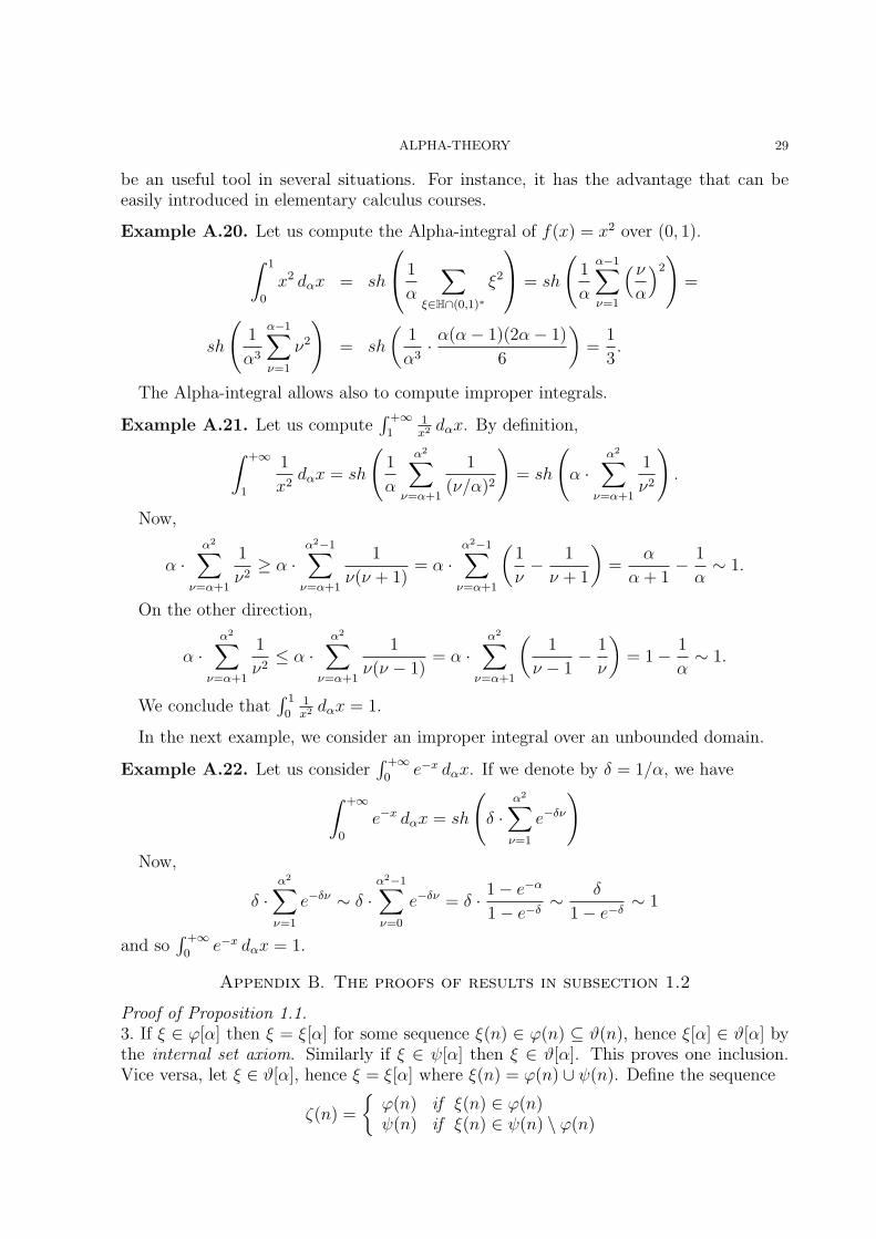
ALPHA-THEORY 29
be an useful tool in several situations. For instance, it has the advantage that can beeasily introduced in elementary calculus courses.
Example A.20. Let us compute the Alpha-integral of f(x) = x2 over (0, 1).
∫ 1
0
x2 dαx = sh
1
α
∑
ξ∈H∩(0,1)∗ξ2
= sh
(1
α
α−1∑ν=1
(ν
α
)2)
=
sh
(1
α3
α−1∑ν=1
ν2
)= sh
(1
α3· α(α− 1)(2α− 1)
6
)=
1
3.
The Alpha-integral allows also to compute improper integrals.
Example A.21. Let us compute∫ +∞1
1x2 dαx. By definition,
∫ +∞
1
1
x2dαx = sh
(1
α
α2∑ν=α+1
1
(ν/α)2
)= sh
(α ·
α2∑ν=α+1
1
ν2
).
Now,
α ·α2∑
ν=α+1
1
ν2≥ α ·
α2−1∑ν=α+1
1
ν(ν + 1)= α ·
α2−1∑ν=α+1
(1
ν− 1
ν + 1
)=
α
α + 1− 1
α∼ 1.
On the other direction,
α ·α2∑
ν=α+1
1
ν2≤ α ·
α2∑ν=α+1
1
ν(ν − 1)= α ·
α2∑ν=α+1
(1
ν − 1− 1
ν
)= 1− 1
α∼ 1.
We conclude that∫ 1
01x2 dαx = 1.
In the next example, we consider an improper integral over an unbounded domain.
Example A.22. Let us consider∫ +∞
0e−x dαx. If we denote by δ = 1/α, we have
∫ +∞
0
e−x dαx = sh
(δ ·
α2∑ν=1
e−δν
)
Now,
δ ·α2∑
ν=1
e−δν ∼ δ ·α2−1∑ν=0
e−δν = δ · 1− e−α
1− e−δ∼ δ
1− e−δ∼ 1
and so∫ +∞
0e−x dαx = 1.
Appendix B. The proofs of results in subsection 1.2
Proof of Proposition 1.1.3. If ξ ∈ ϕ[α] then ξ = ξ[α] for some sequence ξ(n) ∈ ϕ(n) ⊆ ϑ(n), hence ξ[α] ∈ ϑ[α] bythe internal set axiom. Similarly if ξ ∈ ψ[α] then ξ ∈ ϑ[α]. This proves one inclusion.Vice versa, let ξ ∈ ϑ[α], hence ξ = ξ[α] where ξ(n) = ϕ(n) ∪ ψ(n). Define the sequence
ζ(n) =
ϕ(n) if ξ(n) ∈ ϕ(n)ψ(n) if ξ(n) ∈ ψ(n) \ ϕ(n)
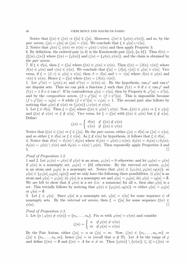
30 VIERI BENCI AND MAURO DI NASSO
Notice that ξ(n) ∈ ζ(n) ⇒ ξ[α] ∈ ζ[α]. Moreover, ζ(n) ∈ ϕ(n), ψ(n), and so, by thepair axiom, ζ[α] = ϕ[α] or ζ[α] = ψ[α]. We conclude that ξ ∈ ϕ[α] ∪ ψ[α].2. Notice that ϕ(n) ⊆ ψ(n) ⇔ ψ(n) = ϕ(n) ∪ ψ(n) and then apply Property 3.6. By definition, the ordered pair 〈a, b〉 is the Kuratowski pair a, a, b. Thus ϑ(n) =ξ(n), ζ(n) where ξ(n) = ϕ(n) and ζ(n) = ϕ(n), ψ(n), and the claim is obtained bythe pair axiom.7. If ξ ∈ ϑ[α], then ξ = ξ[α] where ξ(n) ∈ ϕ(n)× ψ(n). Then ξ(n) = 〈β(n), γ(n)〉 whereβ(n) ∈ ϕ(n) and γ(n) ∈ ψ(n). We conclude that ξ[α] = 〈β[α], γ[α]〉 ∈ ϕ[α] × ψ[α]. Viceversa, if ξ = 〈β, γ〉 ∈ ϕ[α] × ψ[α], then β = β[α] and γ = γ[α] where β(n) ∈ ϕ(n) andγ(n) ∈ ψ(n). Hence ξ = ξ[α] where ξ(n) = 〈β(n), γ(n)〉.1. Let ϕ′(n) = 〈ϕ(n), n〉 and ψ′(n) = 〈ψ(n), n〉. By the hypothesis, ran ϕ′ and ran ψ′
are disjoint sets. Thus we can pick a function f such that f(x) = 0 if x ∈ ran ϕ′ andf(x) = 1 if x ∈ ran ψ′. If by contradiction ϕ[α] = ψ[α], then by Property 6, ϕ′[α] = ψ′[α],and by the composition axiom, (f ϕ′)[α] = (f ψ′)[α]. This is impossible because(f ϕ′)[α] = c0[α] = 0 while (f ψ′)[α] = c1[α] = 1. The second part also follows bynoticing that ϕ(n) /∈ ψ(n) ⇔ ϕ(n) ∪ ψ(n) 6= ψ(n).5. Let ξ ∈ ϑ[α]. Then ξ = ξ[α] where ξ(n) ∈ ϕ(n) \ ψ(n). Now, ξ(n) ∈ ϕ(n) ⇒ ξ ∈ ϕ[α];and ξ(n) /∈ ψ(n) ⇒ ξ /∈ ψ[α]. Vice versa, let ξ = ξ[α] with ξ(n) ∈ ϕ(n) but ξ /∈ ψ[α].Define:
ζ(n) =
ϑ(n) if ξ(n) /∈ ψ(n)ψ(n) if ξ(n) ∈ ψ(n)
Notice that ξ(n) ∈ ζ(n) ⇒ ξ ∈ ζ[α]. By the pair axiom, either ζ[α] = ϑ[α] or ζ[α] = ψ[α],and so either ξ ∈ ϑ[α] or ξ ∈ ψ[α]. As ξ /∈ ψ[α] by hypothesis, it follows that ξ ∈ ϑ[α].4. Notice that ϑ(n) = ϑ1(n) \ ϑ2(n) where ϑ1(n) = ϕ(n) ∪ ψ(n); ϑ2(n) = ϑ3(n) ∪ ϑ4(n);ϑ3(n) = ϕ(n) \ ψ(n) and ϑ4(n) = ψ(n) \ ϕ(n). Then repeatedly apply Properties 3 and5. ¤Proof of Proposition 1.2.1 and 2. Let ϕ1(n) = ϕ(n) if ϕ(n) is an atom, ϕ1(n) = 0 otherwise; and let ϕ2(n) = ϕ(n)if ϕ(n) is a nonempty set, ϕ2(n) = 0 otherwise. By the internal set axiom, ϕ1[α]is an atom and ϕ2[α] is a nonempty set. Notice that ϕ(n) ∈ ϕ1(n), ϕ2(n), c∅(n), soϕ[α] ∈ ϕ1[α], ϕ2[α], c∅[α] and we only have the following three possibilities. i) ϕ[α] is anatom and ϕ[α] = ϕ1[α]; ii) ϕ[α] is a nonempty set and ϕ[α] = ϕ2[α]; iii) ϕ[α] = c∅[α] = ∅.We are left to show that if ϕ(n) is a set (i.e. a nonatom) for all n, then also ϕ[α] is aset. This trivially follows by noticing that ϕ(n) ∈ ϕ2(n), c∅(n) ⇒ either ϕ[α] = ϕ2[α]or ϕ[α] = ∅.3. Let ξ ∈ ϕ[α]. Since ϕ[α] is a nonempty set, ϕ[α] = ψ[α] for some sequence ψ ofnonempty sets. By the internal set axiom, then ξ = ξ[α] for some sequence ξ(n) ∈ψ(n). ¤Proof of Proposition 1.3.1. Let n | ϕ(n) 6= ψ(n) = n1, . . . , nk. Fix m with ϕ(m) = ψ(m) and consider
ζ(n) =
n if ϕ(n) 6= ψ(n)m if ϕ(n) = ψ(n)
By the Pair Axiom, either ζ[α] = α or ζ[α] = m. Now, ζ(n) ∈ n1, . . . , nk,m ⇒ζ[α] ∈ n1, . . . , nk,m, hence ζ[α] = m (recall that α /∈ N). Let A be the range of ϕand define ξ(m) = ∅ and ξ(n) = A for n 6= m. Then ϕ(n) \ ψ(n) ⊆ (ξ ζ)(n) ⇒
ALPHA-THEORY 31
ϕ[α]\ψ[α] ⊆ (ξζ)[α]. But ζ[α] = cm[α] and so, by the composition axiom, (ξζ)[α] =(ξ cm)[α] = c∅[α] = ∅. We conclude that ϕ[α] = ψ[α].2. By the hypothesis ϕ(n)\ψ(n) = ϕ(n) for all but finitely many n. Then ϕ[α]\ψ[α] = ϕ[α] and so ϕ[α] 6= ψ[α]. ¤Proof of Proposition 1.4.Assume first that ϕ[α] = ψ[α] and Λ = n | ϕ(n) = ψ(n). Define ϑ(n) = ξ(n) =ζ(n) if n ∈ Λ and ϑ(n) = ∅ otherwise. Now, (ϕ(n) \ ψ(n)) ∪ ϑ(n) 6= ∅ ⇒(ϕ[α] \ ψ[α]) ∪ ϑ[α] = ϑ[α] 6= ∅ and so it must be ϑ[α] = ξ[α] = ζ[α], henceξ[α] = ζ[α]. The other properties follows by noticing the following facts: ξ(n) 6= ζ(n) ⇔ξ(n) ∩ ζ(n) = ∅, ξ(n) ∈ ζ(n) ⇔ ξ(n) ∩ ζ(n) = ξ(n), and ξ(n) /∈ ζ(n) ⇔ξ(n) ∩ ζ(n) = ∅, respectively.If ϕ[α] 6= ψ[α] and Λ = n | ϕ(n) 6= ψ(n), let ϑ(n) = ϕ(n) ∩ ψ(n). Then ϑ[α] =ϕ[α] ∩ ψ[α] = ∅ = c∅[α], n | ϑ(n) = c∅(n) = Λ, and the claim directly follows fromthe above proofs. ¤
References
[1] L.O. Arkeryd, N.J. Cutland and C.W. Henson, eds., Nonstandard Analysis - Theory and Applica-tions, NATO ASI Series C 493, Kluwer Academic Publishers, 1997.
[2] D. Ballard and K. Hrbacek, Standard foundations for nonstandard analysis, J. Symb. Logic, 57(1992), 471–478.
[3] V. Benci, A construction of a nonstandard universe, in Advances in Dynamical Systems and Quan-tum Physics, S. Albeverio et al. eds., World Scientific, 1995, 207–237.
[4] V. Benci, An algebraic approach to nonstandard analysis, in Calculus of Variations and PartialDifferential Equations, G. Buttazzo, A. Marino and M.K.V. Murthy, eds., Springer-Verlag, 1999,285–326.
[5] V. Benci and M. Di Nasso, A ring homomorphism is enough to get nonstandard analysis, Bull. Belg.Math. Soc. (accepted for publication).
[6] V. Benci and M. Di Nasso, Numerosities of labelled sets: a new way of counting, Advances in Math.,173 (2003), 50–67.
[7] V. Benci and M. Di Nasso, book in preparation.[8] M. Benedikt, Ultrafilters which extend measures, J. Symb. Logic, 63 (1998), 638–662.[9] A. Blass, The Rudin-Keisler ordering of P -points, Trans. Am. Math. Soc., 179 (1973), 145–166.
[10] A. Blass, Ultrafilters: where topological dynamics = algebra = combinatorics, Topology Proc., 18(1993), 33–56.
[11] M. Boffa, Forcing et negation de l’axiome de fondement, Mem. Acad. Sc. Belg., tome XL, fasc. 7,1972.
[12] D. Booth, Ultrafilters on a countable set, Ann. of Math. Logic, 2 (1970), 1–24.[13] C.C. Chang and H.J. Keisler, Model Theory (3rd edition), North-Holland, 1990.[14] G. Choquet, Construction d’ultrafiltres sur N, Bull. Sc. Math., 92 (1968), 41–48.[15] G. Choquet, Deux classes remarquables d’ultrafiltres sur N, Bull. Sc. Math., 92 (1968), 143–153.[16] J. Cleave, Cauchy, convergence and continuity, Brit. J. Phil. Sci., 22 (1971), 27–37.[17] J. Cleave, The concept of ‘variable’ in nineteenth century analysis, Brit. J. Phil. Sci., 30 (1979),
266–278.[18] N. Cutland, Loeb Measures in Practice: Recent Advances, Lecture Notes in Mathematics 1751,
Springer, 2000.[19] N.J. Cutland, C. Kessler, E. Kopp and D. Ross, On Cauchy’s notion of infinitesimal, Brit. J. Phil.
Sci., 39 (1988), 375–378.[20] M. Davis, Applied Nonstandard Analysis, John Wiley & Sons, 1977.[21] M. Di Nasso, On the foundations of nonstandard mathematics, Math. Japonica, 50 (1999), 131–160.[22] M. Di Nasso, An axiomatic presentation of the nonstandard methods in mathematics, J. Symb. Logic,
67 (2002), 315–325.
32 VIERI BENCI AND MAURO DI NASSO
[23] M. Di Nasso, Nonstandard analysis by means of ideal values of sequences, in [49], 63–73.[24] M. Di Nasso, Elementary embeddings of the universe in a nonwellfounded context, in preparation.
[Abstract: Bull. Symb. Logic, 7 (2001), 138.][25] U. Felgner, Comparison of the axioms of local and universal choice, Fund. Math., 71 (1971), 43–62.[26] G. Fisher, Cauchy and the infinitesimally small, Historia Math., 5 (1978), 313–338.[27] G. Fisher, Cauchy’s variables and orders of the infinitesimally small, Brit. J. Phil. Sci., 30 (1979),
361–365.[28] R. Goldblatt, Lectures on the Hyperreals - An Introduction to Nonstandard Analysis, Springer, Grad-
uate Texts in Mathematics 188, 1998.[29] W.S. Hatcher, Calculus is algebra, Am. Math. Monthly, 98 (1982), 362–370.[30] J.M. Henle, Non-nonstandard analysis: real infinitesimals, Math. Intelligencer, 21 (1999), 67–73.[31] C.W. Henson, A gentle introduction to nonstandard extensions, in [1], 1–49.[32] W. Hodges, Model Theory, Cambridge University Press, 1993.[33] T. Jech, Set Theory, Academic Press, 1978.[34] R. Jin, Applications of nonstandard analysis in additive number theory, Bull. Symb. Logic, 6 (2000),
331–341.[35] H.J. Keisler, Foundations of Infinitesimal Calculus, Prindle, Weber and Schmidt, 1976.[36] H.J. Keisler, Elementary Calculus, Prindle, Weber and Schmidt, 1976.[37] K. Kunen, Set Theory. An Introduction to Independence Proofs, North-Holland, 1980.[38] I. Lakatos, Cauchy and the continuum: the significance of non-standard analysis for the history and
philosophy of mathematics, in Mathematics, Science and Epistemology, J. Worrall and G. Currieseds., Philosophical Papers vol. 2, Cambridge University Press, 1978, 43–60.
[39] D. Laugwitz, The Theory of Infinitesimals. An Introduction to Nonstandard Analysis, AccademiaNazionale dei Lincei, Roma, 1980.
[40] W.A.J. Luxemburg, Non-standard Analysis, Lecture Notes, California Institute of Technology,Pasadena, 1962.
[41] V.A. Molchanov, The use of double nonstandard enlargements in topology, Siberian Math. J., 30(1989), 397–402. [Translated from Sibirskii Matem. Z., 30 (1989), 64–71.]
[42] E. Nelson, Internal set theory. A new approach to nonstandard analysis, Bull. Amer. Math. Soc., 83(1977), 1165–1198.
[43] E. Palmgren, Developments in constructive nonstandard analysis, Bull. Symb. Logic, 4 (1998), 223–271.
[44] A. Robinson, Non-standard analysis, Proc. Roy. Acad. Amsterdam, 64 (= Indag. Math., 23) (1961),432–440.
[45] A. Robinson, Non-standard Analysis, North-Holland, 1966.[46] A. Robinson and E. Zakon, A set-theoretical characterization of enlargements, in: Applications of
Model Theory to Algebra, Analysis and Probability, W.A.J. Luxemburg ed., Holt, Rinehart andWinston, 1969, 109–122.
[47] W. Rudin, Homogeneity problems in the theory of Cech compactifications, Duke Math. J., 23 (1956),409–419.
[48] C. Schmieden and D. Laugwitz, Eine erweiterung der infinitesimalrechnung, Math. Zeitschr., 69(1958), 1–39.
[49] P. Schuster, U. Berger and O. Horst, eds., Reuniting the Antipodes - Constructive and NonstandardViews of the Continuum, Synthese Library 306, Kluwer Academic Publishers, 2001.
[50] S. Shelah, Proper Forcing, Lecture Notes in Mathematics 940, North-Holland, 1982.[51] K.D. Stroyan and W.A.J. Luxemburg, Introduction to the Theory of Infinitesimals, Academic Press,
1976.[52] K.D. Stroyan and J.M. Bayod, Foundations of Infinitesimal Stochastic Analysis, North-Holland,
1986.
Dipartimento di Matematica Applicata “U. Dini”, Universita di Pisa, Italy.E-mail address: [email protected]
Dipartimento di Matematica “L. Tonelli”, Universita di Pisa, Italy.E-mail address: [email protected]