GAM for large datasets and load forecasting

Simon Wood, University of Bath, U.K.

in collaboration with

Yannig Goude, EDF

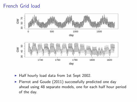
French Grid load

0 500 1000 1500

3050

70

day

GW

1740 1760 1780 1800 1820

3040

50

day

GW

I Half hourly load data from 1st Sept 2002.I Pierrot and Goude (2011) successfully predicted one day

ahead using 48 separate models, one for each half hour periodof the day.

Why 48 models?

I The 48 separate models each have a form something like

MWt = f (MWt−48) +∑

jgj(xjt) + εt

where f and the gj are a smooth functions to be estimated,and the xj are other covariates.

I 48 Separate models has some disadvantages1. Continuity of effects across the day is not enforced.2. Information is wasted as the correlation between neighbouring

time points is not utilised.3. Fitting 48 models, each to 1/48 of the data promotes estimate

instability and creates a huge model checking task each timethe model is updated (every day?)

I But existing methods for fitting such smooth additive modelscould not cope with fitting one model to all the data.

Smooth additive models

I The basic model is

yi =∑

jfj(xji) + εi

where the fj are smooth functions to be estimated.I Need to estimate the fj (including how smooth).I Represent each fj using a spline basis expansion

fj(xj) =∑

k bjk(xj)βjk where bjk are basis functions and βjkare coefficients (maybe 10-100 of each).

I So model becomes

yi =∑

j

∑k

bjk(xji)βjk + εi = Xiβ + εi

. . . a linear model. But it is much too flexible.

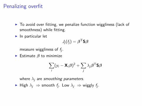
Penalizing overfit

I To avoid over fitting, we penalize function wiggliness (lack ofsmoothness) while fitting.

I In particular letJj(fj) = βTSβ

measure wiggliness of fj .I Estimate β to minimize∑

i(yi − Xiβ)

2 +∑

jλjβ

TSβ

where λj are smoothing parameters.I High λj ⇒ smooth fj . Low λj ⇒ wiggly fj .

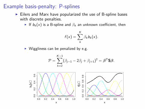
Example basis-penalty: P-splinesI Eilers and Marx have popularized the use of B-spline bases

with discrete penalties.I If bk(x) is a B-spline and βk an unknown coefficient, then

f (x) =K∑k

βkbk(x).

I Wiggliness can be penalized by e.g.

P =K−1∑k=2

(βj−1 − 2βj + βj+1)2 = βTSβ.

0.0 0.2 0.4 0.6 0.8 1.0

0.0

0.2

0.4

0.6

x

b k(x

)

0.0 0.2 0.4 0.6 0.8 1.0

0.0

0.2

0.4

0.6

0.8

x

f(x)

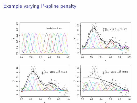
Example varying P-spline penalty

0.0 0.2 0.4 0.6 0.8 1.0

0.0

0.2

0.4

0.6

0.8

1.0

x

y

basis functions

0.0 0.2 0.4 0.6 0.8 1.0

−2

02

46

810

x

y

∑i

(βi−1 − 2βi + βi+1)2 = 207

0.0 0.2 0.4 0.6 0.8 1.0

−2

02

46

810

x

y

∑i

(βi−1 − 2βi + βi+1)2 = 16.4

0.0 0.2 0.4 0.6 0.8 1.0

−2

02

46

810

x

y∑

i(βi−1 − 2βi + βi+1)2 = 0.04

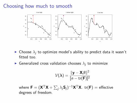
Choosing how much to smooth

0.2 0.4 0.6 0.8 1.0

−2

02

46

8

λ too high

x

y

0.2 0.4 0.6 0.8 1.0

−2

02

46

8

λ about right

x

y

0.2 0.4 0.6 0.8 1.0

−2

02

46

8

λ too low

x

y

I Choose λj to optimize model’s ability to predict data it wasn’tfitted too.

I Generalized cross validation chooses λj to minimize

V(λ) = ‖y − Xβ‖2

[n − tr(F)]2

where F = (XTX +∑

j λjSj)−1XTX. tr(F) = effective

degrees of freedom.

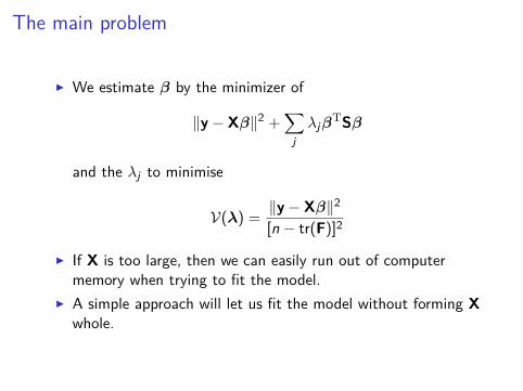
The main problem

I We estimate β by the minimizer of

‖y − Xβ‖2 +∑

jλjβ

TSβ

and the λj to minimise

V(λ) = ‖y − Xβ‖2

[n − tr(F)]2

I If X is too large, then we can easily run out of computermemory when trying to fit the model.

I A simple approach will let us fit the model without forming Xwhole.

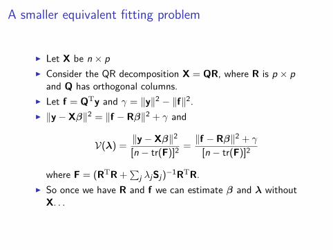
A smaller equivalent fitting problem

I Let X be n × pI Consider the QR decomposition X = QR, where R is p × p

and Q has orthogonal columns.I Let f = QTy and γ = ‖y‖2 − ‖f‖2.I ‖y − Xβ‖2 = ‖f − Rβ‖2 + γ and

V(λ) = ‖y − Xβ‖2

[n − tr(F)]2 =‖f − Rβ‖2 + γ

[n − tr(F)]2

where F = (RTR +∑

j λjSj)−1RTR.

I So once we have R and f we can estimate β and λ withoutX. . .

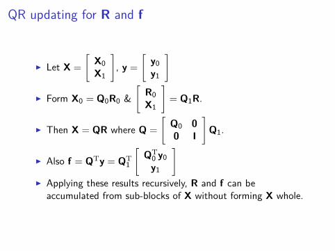
QR updating for R and f

I Let X =

[X0X1

], y =

[y0y1

]

I Form X0 = Q0R0 &[

R0X1

]= Q1R.

I Then X = QR where Q =

[Q0 00 I

]Q1.

I Also f = QTy = QT1

[QT

0 y0y1

]I Applying these results recursively, R and f can be

accumulated from sub-blocks of X without forming X whole.

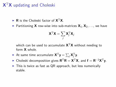
XTX updating and Choleski

I R is the Choleski factor of XTX.I Partitioning X row-wise into sub-matrices X1, X2, . . ., we have

XTX =∑

jXT

j Xj

which can be used to accumulate XTX without needing toform X whole.

I At same time accumulate XTy =∑

j XTj y.

I Choleski decomposition gives RTR = XTX, and f = R−1XTy.I This is twice as fast as QR approach, but less numerically

stable.

Generalizations

1. Generalized additive models (GAMs) allow distributions otherthan normal (and non-identity link functions).

2. GAMs can be estimated by iteratively estimating workinglinear models, using R and f accumulation tricks on each.

3. REML, AIC etc can also be used for λj estimation. REML canbe made especially efficient in this context.

4. The accumulation methods are easy to parallelize.5. Updating a model fit with new data is very easy.6. AR1 residuals can also be handled easily in the

non-generalized case.

Air pollution example

I Around 5000 daily death rates, for Chicago, along with time,ozone, pm10, tmp (last 3 averaged over preceding 3 days).Peng and Welty (2004).

I Appropriate GAM is: deathi ∼ Poi,

log{E(deathi)} = f1(timei) + f2(ozonei , tmpi) + f3(pm10i).

I f1 and f3 penalized cubic regression splines, f2 tensor productspline.

I Results suggest a very strong ozone - temperature interaction.

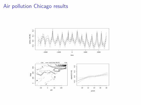
Air pollution Chicago results

−2000 −1000 0 1000 2000

−0.

10.

00.

10.

2

time

s(tim

e,13

6.85

)

te(o3,tmp,38.63)

−50 0 50 100

010

020

030

0

o3

tmp

−1se +1se

10 12 14 16 18

−0.

10.

00.

10.

2

pm10

s(pm

10,3

.42)

Air pollution Chicago results

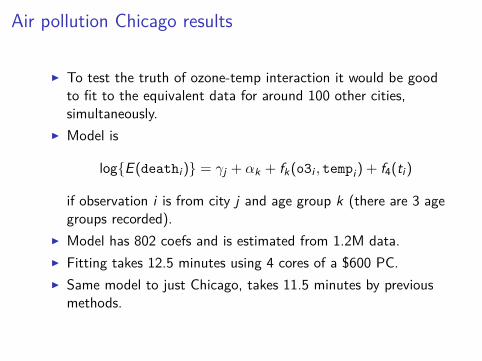
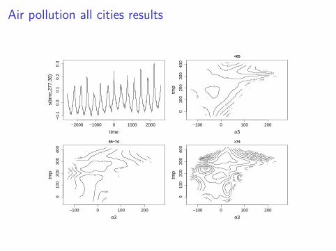
I To test the truth of ozone-temp interaction it would be goodto fit to the equivalent data for around 100 other cities,simultaneously.

I Model is

log{E (deathi)} = γj + αk + fk(o3i , tempi) + f4(ti)

if observation i is from city j and age group k (there are 3 agegroups recorded).

I Model has 802 coefs and is estimated from 1.2M data.I Fitting takes 12.5 minutes using 4 cores of a $600 PC.I Same model to just Chicago, takes 11.5 minutes by previous

methods.

Air pollution all cities results

−2000 −1000 0 1000 2000

−0.

10.

00.

10.

20.

3

time

s(tim

e,27

7.36

)<65

o3

tmp

−0.5

−0.3 −0.2

−0.2 −0.2

−0.1

−0.1

−0.1

0

0

0

0

0.1 0.2

0.3

−100 0 100 200

010

020

030

040

0

65−74

o3

tmp

−0.05

0

0

0

0.05

0.05

0.05

0.1

0.1

0.1

0.15

0.15

−100 0 100 200

010

020

030

040

0

>74

o3

tmp

−0.02

−0.02

0

0

0

0

0.02

0.0

2

0.02

0.04 0.04 0.04

0.0

4

0.04

0.04

0.06

0.06

0.06

0.06

0.06 0.08

0.08

0.08

0.1

0.12 0.14

−100 0 100 200

010

020

030

040

0

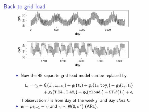
Back to grid load

0 500 1000 1500

3050

70

day

GW

1740 1760 1780 1800 1820

3040

50

day

GW

I Now the 48 separate grid load model can be replaced by

Li = γj + fk(Ii , Li−48) + g1(ti) + g2(Ii , toyi) + g3(Ti , Ii)

+ g4(T.24i , T.48i) + g5(cloudi) + STih(Ii) + ei

if observation i is from day of the week j, and day class k.I ei = ρei−1 + εi and εi ∼ N(0, σ2) (AR1).

Fitting grid load model

I Using QR update fitting takes under 30 minutes and weestimate ρ = 0.98.

I Update with new data then takes under 2 minutes.I We fit up to 31 August 2008, and then predicted the next

years data, one day at a time, with model update.I Predictive RMSE was 1156MW (1024MW for fit). Predictive

MAPE 1.62% (1.46% for fit).I Setting ρ = 0 gives overfit, and worse predictive performance.

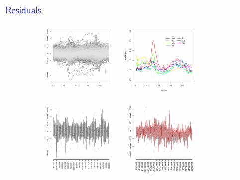
Residuals

0 10 20 30 40

−60

00−

2000

020

0040

0060

00

0 10 20 30 40

0.5

1.0

1.5

2.0

2.5

3.0

Instant

MA

PE

(%

)

MoTuWeTh

FrSaSu

9/1/

2002

12/1

9/20

02

4/8/

2003

8/12

/200

3

12/4

/200

3

3/22

/200

4

7/26

/200

4

11/1

7/20

04

3/7/

2005

7/6/

2005

10/2

3/20

05

2/18

/200

6

6/20

/200

6

10/8

/200

6

2/3/

2007

6/4/

2007

9/21

/200

7

1/17

/200

8

5/6/

2008

8/31

/200

8

−60

00−

2000

020

0040

0060

00

1/9/

2008

17/9

/200

84/

10/2

008

21/1

0/20

0815

/11/

2008

2/12

/200

819

/12/

2008

13/1

/200

930

/1/2

009

16/2

/200

94/

3/20

0921

/3/2

009

7/4/

2009

28/4

/200

927

/5/2

009

17/6

/200

94/

7/20

0925

/7/2

009

11/8

/200

931

/8/2

009

−60

00−

4000

−20

000

2000

4000

6000

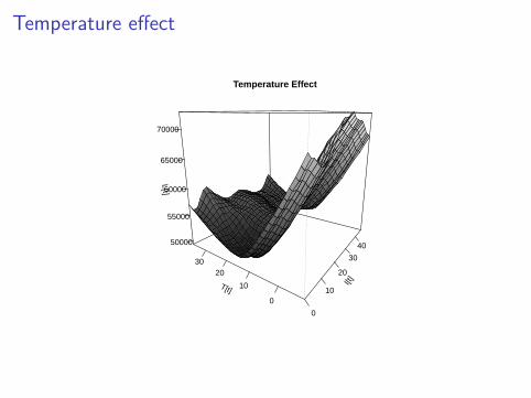
Temperature effect

I[t]

0

10

20

30

40

T[t]0

10

2030

L[t]

50000

55000

60000

65000

70000

Temperature Effect

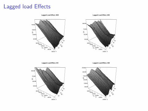
Lagged load Effects

I[t]

0

10

20

30

40

L[t − 1]

30000

40000

5000060000

7000080000

L[t]

40000

50000

60000

70000

Lagged Load Effect, WW

I[t]

0

10

20

30

40

L[t − 1]

30000

40000

5000060000

7000080000

L[t]

50000

60000

70000

80000

Lagged Load Effect, WH

I[t]

0

10

20

30

40

L[t − 1]

30000

40000

5000060000

7000080000

L[t]

50000

60000

70000

80000

Lagged Load Effect, HH

I[t]

0

10

20

30

40

L[t − 1]

30000

40000

5000060000

7000080000

L[t]

40000

50000

60000

70000

80000

90000

Lagged Load Effect, HW