BABAR-CONF-2006/037SLAC-PUB-12035

hep-ex/0608002July 2006

Measurement of CP-Violating Asymmetries in B0 → (ρπ)0

Using a Time-Dependent Dalitz Plot Analysis

The BABAR Collaboration

July 31, 2006

Abstract

We report a measurement of CP -violating asymmetries in B0 → (ρπ)0 → π+π−π0 decaysusing a time-dependent Dalitz plot analysis. The results are obtained from a data sample of 347million Υ (4S) → BB decays, collected by the BABAR detector at the PEP-II asymmetric-energyB Factory at SLAC. We measure 26 coefficients of the bilinear form factor terms occurring in thetime-dependent decay rate of the B0 meson and derive the physically relevant quantities from thesecoefficients. In particular we find a three standard deviation evidence of direct CP -violation in theB0 → ρ±π∓ decays, with systematic uncertainties included. We also achieve a constraint of theangle α of the Unitarity Triangle. All results presented are preliminary.

Submitted to the 33rd International Conference on High-Energy Physics, ICHEP 06,26 July—2 August 2006, Moscow, Russia.

Stanford Linear Accelerator Center, Stanford University, Stanford, CA 94309Work supported in part by Department of Energy contract DE-AC02-76SF00515.

1

The BABAR Collaboration,

B. Aubert, R. Barate, M. Bona, D. Boutigny, F. Couderc, Y. Karyotakis, J. P. Lees, V. Poireau,V. Tisserand, A. Zghiche

Laboratoire de Physique des Particules, IN2P3/CNRS et Universite de Savoie, F-74941 Annecy-Le-Vieux,France

E. Grauges

Universitat de Barcelona, Facultat de Fisica, Departament ECM, E-08028 Barcelona, Spain

A. Palano

Universita di Bari, Dipartimento di Fisica and INFN, I-70126 Bari, Italy

J. C. Chen, N. D. Qi, G. Rong, P. Wang, Y. S. Zhu

Institute of High Energy Physics, Beijing 100039, China

G. Eigen, I. Ofte, B. Stugu

University of Bergen, Institute of Physics, N-5007 Bergen, Norway

G. S. Abrams, M. Battaglia, D. N. Brown, J. Button-Shafer, R. N. Cahn, E. Charles, M. S. Gill,Y. Groysman, R. G. Jacobsen, J. A. Kadyk, L. T. Kerth, Yu. G. Kolomensky, G. Kukartsev, G. Lynch,

L. M. Mir, T. J. Orimoto, M. Pripstein, N. A. Roe, M. T. Ronan, W. A. Wenzel

Lawrence Berkeley National Laboratory and University of California, Berkeley, California 94720, USA

P. del Amo Sanchez, M. Barrett, K. E. Ford, A. J. Hart, T. J. Harrison, C. M. Hawkes, S. E. Morgan,A. T. Watson

University of Birmingham, Birmingham, B15 2TT, United Kingdom

T. Held, H. Koch, B. Lewandowski, M. Pelizaeus, K. Peters, T. Schroeder, M. Steinke

Ruhr Universitat Bochum, Institut fur Experimentalphysik 1, D-44780 Bochum, Germany

J. T. Boyd, J. P. Burke, W. N. Cottingham, D. Walker

University of Bristol, Bristol BS8 1TL, United Kingdom

D. J. Asgeirsson, T. Cuhadar-Donszelmann, B. G. Fulsom, C. Hearty, N. S. Knecht, T. S. Mattison,J. A. McKenna

University of British Columbia, Vancouver, British Columbia, Canada V6T 1Z1

A. Khan, P. Kyberd, M. Saleem, D. J. Sherwood, L. Teodorescu

Brunel University, Uxbridge, Middlesex UB8 3PH, United Kingdom

V. E. Blinov, A. D. Bukin, V. P. Druzhinin, V. B. Golubev, A. P. Onuchin, S. I. Serednyakov,Yu. I. Skovpen, E. P. Solodov, K. Yu Todyshev

Budker Institute of Nuclear Physics, Novosibirsk 630090, Russia

D. S. Best, M. Bondioli, M. Bruinsma, M. Chao, S. Curry, I. Eschrich, D. Kirkby, A. J. Lankford, P. Lund,M. Mandelkern, R. K. Mommsen, W. Roethel, D. P. Stoker

University of California at Irvine, Irvine, California 92697, USA

S. Abachi, C. Buchanan

University of California at Los Angeles, Los Angeles, California 90024, USA

2

S. D. Foulkes, J. W. Gary, O. Long, B. C. Shen, K. Wang, L. Zhang

University of California at Riverside, Riverside, California 92521, USA

H. K. Hadavand, E. J. Hill, H. P. Paar, S. Rahatlou, V. Sharma

University of California at San Diego, La Jolla, California 92093, USA

J. W. Berryhill, C. Campagnari, A. Cunha, B. Dahmes, T. M. Hong, D. Kovalskyi, J. D. Richman

University of California at Santa Barbara, Santa Barbara, California 93106, USA

T. W. Beck, A. M. Eisner, C. J. Flacco, C. A. Heusch, J. Kroseberg, W. S. Lockman, G. Nesom, T. Schalk,B. A. Schumm, A. Seiden, P. Spradlin, D. C. Williams, M. G. Wilson

University of California at Santa Cruz, Institute for Particle Physics, Santa Cruz, California 95064, USA

J. Albert, E. Chen, A. Dvoretskii, F. Fang, D. G. Hitlin, I. Narsky, T. Piatenko, F. C. Porter, A. Ryd,A. Samuel

California Institute of Technology, Pasadena, California 91125, USA

G. Mancinelli, B. T. Meadows, K. Mishra, M. D. Sokoloff

University of Cincinnati, Cincinnati, Ohio 45221, USA

F. Blanc, P. C. Bloom, S. Chen, W. T. Ford, J. F. Hirschauer, A. Kreisel, M. Nagel, U. Nauenberg,A. Olivas, W. O. Ruddick, J. G. Smith, K. A. Ulmer, S. R. Wagner, J. Zhang

University of Colorado, Boulder, Colorado 80309, USA

A. Chen, E. A. Eckhart, A. Soffer, W. H. Toki, R. J. Wilson, F. Winklmeier, Q. Zeng

Colorado State University, Fort Collins, Colorado 80523, USA

D. D. Altenburg, E. Feltresi, A. Hauke, H. Jasper, J. Merkel, A. Petzold, B. Spaan

Universitat Dortmund, Institut fur Physik, D-44221 Dortmund, Germany

T. Brandt, V. Klose, H. M. Lacker, W. F. Mader, R. Nogowski, J. Schubert, K. R. Schubert, R. Schwierz,J. E. Sundermann, A. Volk

Technische Universitat Dresden, Institut fur Kern- und Teilchenphysik, D-01062 Dresden, Germany

D. Bernard, G. R. Bonneaud, E. Latour, Ch. Thiebaux, M. Verderi

Laboratoire Leprince-Ringuet, CNRS/IN2P3, Ecole Polytechnique, F-91128 Palaiseau, France

P. J. Clark, W. Gradl, F. Muheim, S. Playfer, A. I. Robertson, Y. Xie

University of Edinburgh, Edinburgh EH9 3JZ, United Kingdom

M. Andreotti, D. Bettoni, C. Bozzi, R. Calabrese, G. Cibinetto, E. Luppi, M. Negrini, A. Petrella,L. Piemontese, E. Prencipe

Universita di Ferrara, Dipartimento di Fisica and INFN, I-44100 Ferrara, Italy

F. Anulli, R. Baldini-Ferroli, A. Calcaterra, R. de Sangro, G. Finocchiaro, S. Pacetti, P. Patteri,I. M. Peruzzi,1 M. Piccolo, M. Rama, A. Zallo

Laboratori Nazionali di Frascati dell’INFN, I-00044 Frascati, Italy1Also with Universita di Perugia, Dipartimento di Fisica, Perugia, Italy

3

A. Buzzo, R. Capra, R. Contri, M. Lo Vetere, M. M. Macri, M. R. Monge, S. Passaggio, C. Patrignani,E. Robutti, A. Santroni, S. Tosi

Universita di Genova, Dipartimento di Fisica and INFN, I-16146 Genova, Italy

G. Brandenburg, K. S. Chaisanguanthum, M. Morii, J. Wu

Harvard University, Cambridge, Massachusetts 02138, USA

R. S. Dubitzky, J. Marks, S. Schenk, U. Uwer

Universitat Heidelberg, Physikalisches Institut, Philosophenweg 12, D-69120 Heidelberg, Germany

D. J. Bard, W. Bhimji, D. A. Bowerman, P. D. Dauncey, U. Egede, R. L. Flack, J. A. Nash,M. B. Nikolich, W. Panduro Vazquez

Imperial College London, London, SW7 2AZ, United Kingdom

P. K. Behera, X. Chai, M. J. Charles, U. Mallik, N. T. Meyer, V. Ziegler

University of Iowa, Iowa City, Iowa 52242, USA

J. Cochran, H. B. Crawley, L. Dong, V. Eyges, W. T. Meyer, S. Prell, E. I. Rosenberg, A. E. Rubin

Iowa State University, Ames, Iowa 50011-3160, USA

A. V. Gritsan

Johns Hopkins University, Baltimore, Maryland 21218, USA

A. G. Denig, M. Fritsch, G. Schott

Universitat Karlsruhe, Institut fur Experimentelle Kernphysik, D-76021 Karlsruhe, Germany

N. Arnaud, M. Davier, G. Grosdidier, A. Hocker, F. Le Diberder, V. Lepeltier, A. M. Lutz, A. Oyanguren,S. Pruvot, S. Rodier, P. Roudeau, M. H. Schune, A. Stocchi, W. F. Wang, G. Wormser

Laboratoire de l’Accelerateur Lineaire, IN2P3/CNRS et Universite Paris-Sud 11, Centre Scientifiqued’Orsay, B.P. 34, F-91898 ORSAY Cedex, France

C. H. Cheng, D. J. Lange, D. M. Wright

Lawrence Livermore National Laboratory, Livermore, California 94550, USA

C. A. Chavez, I. J. Forster, J. R. Fry, E. Gabathuler, R. Gamet, K. A. George, D. E. Hutchcroft,D. J. Payne, K. C. Schofield, C. Touramanis

University of Liverpool, Liverpool L69 7ZE, United Kingdom

A. J. Bevan, F. Di Lodovico, W. Menges, R. Sacco

Queen Mary, University of London, E1 4NS, United Kingdom

G. Cowan, H. U. Flaecher, D. A. Hopkins, P. S. Jackson, T. R. McMahon, S. Ricciardi, F. Salvatore,A. C. Wren

University of London, Royal Holloway and Bedford New College, Egham, Surrey TW20 0EX, UnitedKingdom

D. N. Brown, C. L. Davis

University of Louisville, Louisville, Kentucky 40292, USA

4

J. Allison, N. R. Barlow, R. J. Barlow, Y. M. Chia, C. L. Edgar, G. D. Lafferty, M. T. Naisbit,J. C. Williams, J. I. Yi

University of Manchester, Manchester M13 9PL, United Kingdom

C. Chen, W. D. Hulsbergen, A. Jawahery, C. K. Lae, D. A. Roberts, G. Simi

University of Maryland, College Park, Maryland 20742, USA

G. Blaylock, C. Dallapiccola, S. S. Hertzbach, X. Li, T. B. Moore, S. Saremi, H. Staengle

University of Massachusetts, Amherst, Massachusetts 01003, USA

R. Cowan, G. Sciolla, S. J. Sekula, M. Spitznagel, F. Taylor, R. K. Yamamoto

Massachusetts Institute of Technology, Laboratory for Nuclear Science, Cambridge, Massachusetts 02139,USA

H. Kim, S. E. Mclachlin, P. M. Patel, S. H. Robertson

McGill University, Montreal, Quebec, Canada H3A 2T8

A. Lazzaro, V. Lombardo, F. Palombo

Universita di Milano, Dipartimento di Fisica and INFN, I-20133 Milano, Italy

J. M. Bauer, L. Cremaldi, V. Eschenburg, R. Godang, R. Kroeger, D. A. Sanders, D. J. Summers,H. W. Zhao

University of Mississippi, University, Mississippi 38677, USA

S. Brunet, D. Cote, M. Simard, P. Taras, F. B. Viaud

Universite de Montreal, Physique des Particules, Montreal, Quebec, Canada H3C 3J7

H. Nicholson

Mount Holyoke College, South Hadley, Massachusetts 01075, USA

N. Cavallo,2 G. De Nardo, F. Fabozzi,3 C. Gatto, L. Lista, D. Monorchio, P. Paolucci, D. Piccolo,C. Sciacca

Universita di Napoli Federico II, Dipartimento di Scienze Fisiche and INFN, I-80126, Napoli, Italy

M. A. Baak, G. Raven, H. L. Snoek

NIKHEF, National Institute for Nuclear Physics and High Energy Physics, NL-1009 DB Amsterdam, TheNetherlands

C. P. Jessop, J. M. LoSecco

University of Notre Dame, Notre Dame, Indiana 46556, USA

T. Allmendinger, G. Benelli, L. A. Corwin, K. K. Gan, K. Honscheid, D. Hufnagel, P. D. Jackson,H. Kagan, R. Kass, A. M. Rahimi, J. J. Regensburger, R. Ter-Antonyan, Q. K. Wong

Ohio State University, Columbus, Ohio 43210, USA

N. L. Blount, J. Brau, R. Frey, O. Igonkina, J. A. Kolb, M. Lu, R. Rahmat, N. B. Sinev, D. Strom,J. Strube, E. Torrence

University of Oregon, Eugene, Oregon 97403, USA2Also with Universita della Basilicata, Potenza, Italy3Also with Universita della Basilicata, Potenza, Italy

5

A. Gaz, M. Margoni, M. Morandin, A. Pompili, M. Posocco, M. Rotondo, F. Simonetto, R. Stroili, C. Voci

Universita di Padova, Dipartimento di Fisica and INFN, I-35131 Padova, Italy

M. Benayoun, H. Briand, J. Chauveau, P. David, L. Del Buono, Ch. de la Vaissiere, O. Hamon,B. L. Hartfiel, M. J. J. John, Ph. Leruste, J. Malcles, J. Ocariz, L. Roos, G. Therin

Laboratoire de Physique Nucleaire et de Hautes Energies, IN2P3/CNRS, Universite Pierre et MarieCurie-Paris6, Universite Denis Diderot-Paris7, F-75252 Paris, France

L. Gladney, J. Panetta

University of Pennsylvania, Philadelphia, Pennsylvania 19104, USA

M. Biasini, R. Covarelli

Universita di Perugia, Dipartimento di Fisica and INFN, I-06100 Perugia, Italy

C. Angelini, G. Batignani, S. Bettarini, F. Bucci, G. Calderini, M. Carpinelli, R. Cenci, F. Forti,M. A. Giorgi, A. Lusiani, G. Marchiori, M. A. Mazur, M. Morganti, N. Neri, E. Paoloni, G. Rizzo,

J. J. Walsh

Universita di Pisa, Dipartimento di Fisica, Scuola Normale Superiore and INFN, I-56127 Pisa, Italy

M. Haire, D. Judd, D. E. Wagoner

Prairie View A&M University, Prairie View, Texas 77446, USA

J. Biesiada, N. Danielson, P. Elmer, Y. P. Lau, C. Lu, J. Olsen, A. J. S. Smith, A. V. Telnov

Princeton University, Princeton, New Jersey 08544, USA

F. Bellini, G. Cavoto, A. D’Orazio, D. del Re, E. Di Marco, R. Faccini, F. Ferrarotto, F. Ferroni,M. Gaspero, L. Li Gioi, M. A. Mazzoni, S. Morganti, G. Piredda, F. Polci, F. Safai Tehrani, C. Voena

Universita di Roma La Sapienza, Dipartimento di Fisica and INFN, I-00185 Roma, Italy

M. Ebert, H. Schroder, R. Waldi

Universitat Rostock, D-18051 Rostock, Germany

T. Adye, N. De Groot, B. Franek, E. O. Olaiya, F. F. Wilson

Rutherford Appleton Laboratory, Chilton, Didcot, Oxon, OX11 0QX, United Kingdom

R. Aleksan, S. Emery, A. Gaidot, S. F. Ganzhur, G. Hamel de Monchenault, W. Kozanecki, M. Legendre,G. Vasseur, Ch. Yeche, M. Zito

DSM/Dapnia, CEA/Saclay, F-91191 Gif-sur-Yvette, France

X. R. Chen, H. Liu, W. Park, M. V. Purohit, J. R. Wilson

University of South Carolina, Columbia, South Carolina 29208, USA

M. T. Allen, D. Aston, R. Bartoldus, P. Bechtle, N. Berger, R. Claus, J. P. Coleman, M. R. Convery,M. Cristinziani, J. C. Dingfelder, J. Dorfan, G. P. Dubois-Felsmann, D. Dujmic, W. Dunwoodie,

R. C. Field, T. Glanzman, S. J. Gowdy, M. T. Graham, P. Grenier,4 V. Halyo, C. Hast, T. Hryn’ova,W. R. Innes, M. H. Kelsey, P. Kim, D. W. G. S. Leith, S. Li, S. Luitz, V. Luth, H. L. Lynch,

D. B. MacFarlane, H. Marsiske, R. Messner, D. R. Muller, C. P. O’Grady, V. E. Ozcan, A. Perazzo,M. Perl, T. Pulliam, B. N. Ratcliff, A. Roodman, A. A. Salnikov, R. H. Schindler, J. Schwiening,

A. Snyder, J. Stelzer, D. Su, M. K. Sullivan, K. Suzuki, S. K. Swain, J. M. Thompson, J. Va’vra, N. van4Also at Laboratoire de Physique Corpusculaire, Clermont-Ferrand, France

6

Bakel, M. Weaver, A. J. R. Weinstein, W. J. Wisniewski, M. Wittgen, D. H. Wright, A. K. Yarritu, K. Yi,C. C. Young

Stanford Linear Accelerator Center, Stanford, California 94309, USA

P. R. Burchat, A. J. Edwards, S. A. Majewski, B. A. Petersen, C. Roat, L. Wilden

Stanford University, Stanford, California 94305-4060, USA

S. Ahmed, M. S. Alam, R. Bula, J. A. Ernst, V. Jain, B. Pan, M. A. Saeed, F. R. Wappler, S. B. Zain

State University of New York, Albany, New York 12222, USA

W. Bugg, M. Krishnamurthy, S. M. Spanier

University of Tennessee, Knoxville, Tennessee 37996, USA

R. Eckmann, J. L. Ritchie, A. Satpathy, C. J. Schilling, R. F. Schwitters

University of Texas at Austin, Austin, Texas 78712, USA

J. M. Izen, X. C. Lou, S. Ye

University of Texas at Dallas, Richardson, Texas 75083, USA

F. Bianchi, F. Gallo, D. Gamba

Universita di Torino, Dipartimento di Fisica Sperimentale and INFN, I-10125 Torino, Italy

M. Bomben, L. Bosisio, C. Cartaro, F. Cossutti, G. Della Ricca, S. Dittongo, L. Lanceri, L. Vitale

Universita di Trieste, Dipartimento di Fisica and INFN, I-34127 Trieste, Italy

V. Azzolini, N. Lopez-March, F. Martinez-Vidal

IFIC, Universitat de Valencia-CSIC, E-46071 Valencia, Spain

Sw. Banerjee, B. Bhuyan, C. M. Brown, D. Fortin, K. Hamano, R. Kowalewski, I. M. Nugent, J. M. Roney,R. J. Sobie

University of Victoria, Victoria, British Columbia, Canada V8W 3P6

J. J. Back, P. F. Harrison, T. E. Latham, G. B. Mohanty, M. Pappagallo

Department of Physics, University of Warwick, Coventry CV4 7AL, United Kingdom

H. R. Band, X. Chen, B. Cheng, S. Dasu, M. Datta, K. T. Flood, J. J. Hollar, P. E. Kutter, B. Mellado,A. Mihalyi, Y. Pan, M. Pierini, R. Prepost, S. L. Wu, Z. Yu

University of Wisconsin, Madison, Wisconsin 53706, USA

H. Neal

Yale University, New Haven, Connecticut 06511, USA

7

1 INTRODUCTION

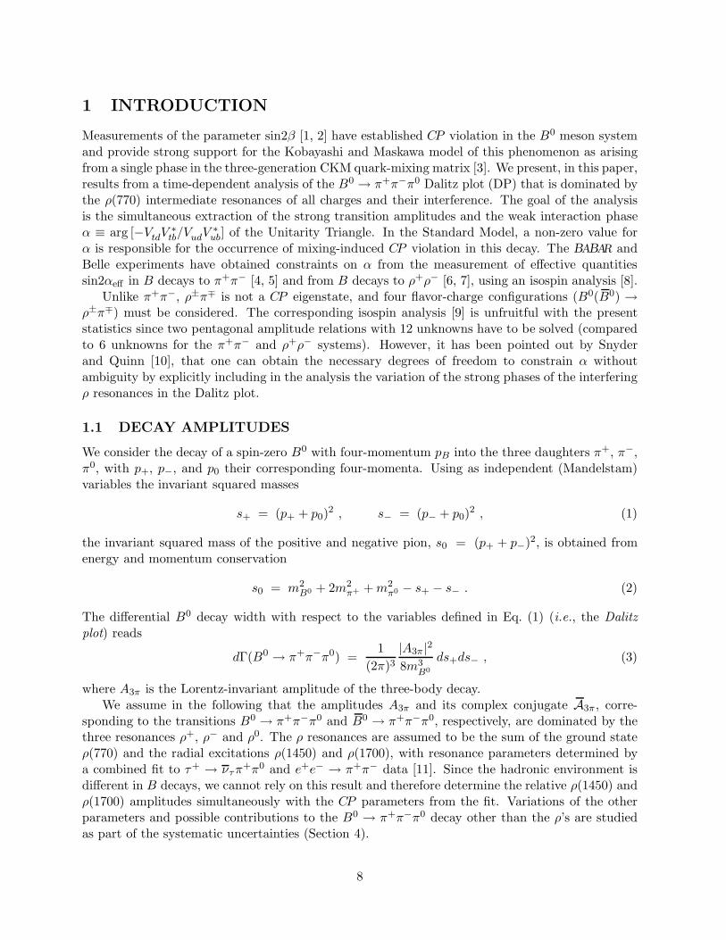
Measurements of the parameter sin2β [1, 2] have established CP violation in the B0 meson systemand provide strong support for the Kobayashi and Maskawa model of this phenomenon as arisingfrom a single phase in the three-generation CKM quark-mixing matrix [3]. We present, in this paper,results from a time-dependent analysis of the B0 → π+π−π0 Dalitz plot (DP) that is dominated bythe ρ(770) intermediate resonances of all charges and their interference. The goal of the analysisis the simultaneous extraction of the strong transition amplitudes and the weak interaction phaseα ≡ arg [−VtdV

∗tb/VudV

∗ub] of the Unitarity Triangle. In the Standard Model, a non-zero value for

α is responsible for the occurrence of mixing-induced CP violation in this decay. The BABAR andBelle experiments have obtained constraints on α from the measurement of effective quantitiessin2αeff in B decays to π+π− [4, 5] and from B decays to ρ+ρ− [6, 7], using an isospin analysis [8].

Unlike π+π−, ρ±π∓ is not a CP eigenstate, and four flavor-charge configurations (B0(B0) →ρ±π∓) must be considered. The corresponding isospin analysis [9] is unfruitful with the presentstatistics since two pentagonal amplitude relations with 12 unknowns have to be solved (comparedto 6 unknowns for the π+π− and ρ+ρ− systems). However, it has been pointed out by Snyderand Quinn [10], that one can obtain the necessary degrees of freedom to constrain α withoutambiguity by explicitly including in the analysis the variation of the strong phases of the interferingρ resonances in the Dalitz plot.

1.1 DECAY AMPLITUDES

We consider the decay of a spin-zero B0 with four-momentum pB into the three daughters π+, π−,π0, with p+, p−, and p0 their corresponding four-momenta. Using as independent (Mandelstam)variables the invariant squared masses

s+ = (p+ + p0)2 , s− = (p− + p0)2 , (1)

the invariant squared mass of the positive and negative pion, s0 = (p+ + p−)2, is obtained fromenergy and momentum conservation

s0 = m2B0 + 2m2

π+ +m2π0 − s+ − s− . (2)

The differential B0 decay width with respect to the variables defined in Eq. (1) (i.e., the Dalitzplot) reads

dΓ(B0 → π+π−π0) =1

(2π)3|A3π|28m3

B0

ds+ds− , (3)

where A3π is the Lorentz-invariant amplitude of the three-body decay.We assume in the following that the amplitudes A3π and its complex conjugate A3π, corre-

sponding to the transitions B0 → π+π−π0 and B0 → π+π−π0, respectively, are dominated by thethree resonances ρ+, ρ− and ρ0. The ρ resonances are assumed to be the sum of the ground stateρ(770) and the radial excitations ρ(1450) and ρ(1700), with resonance parameters determined bya combined fit to τ+ → ντπ

+π0 and e+e− → π+π− data [11]. Since the hadronic environment isdifferent in B decays, we cannot rely on this result and therefore determine the relative ρ(1450) andρ(1700) amplitudes simultaneously with the CP parameters from the fit. Variations of the otherparameters and possible contributions to the B0 → π+π−π0 decay other than the ρ’s are studiedas part of the systematic uncertainties (Section 4).

8

Including the B0B0 mixing parameter q/p into the B0 decay amplitudes, we can write [10, 12]

A3π = f+A+ + f−A− + f0A

0 , (4)A3π = f+A

+ + f−A− + f0A0 , (5)

where the fκ (with κ = {+,−, 0} denote the charge of the ρ from the decay of the B0 meson)are functions of the Dalitz variables s+ and s− that incorporate the kinematic and dynamicalproperties of the B0 decay into a (vector) ρ resonance and a (pseudoscalar) pion, and where theAκ are complex amplitudes that may comprise weak and strong transition phases and that areindependent of the Dalitz variables. Note that the definitions (4) and (5) imply the assumptionthat the relative phases between the ρ(770) and its radial excitations are CP -conserving.

Following Ref. [11], the ρ resonances are parameterized in fκ by a modified relativistic Breit-Wigner function introduced by Gounaris and Sakurai (GS) [15]. Due to angular momentum con-servation, the spin-one ρ resonance is polarized in a helicity-zero state. For a ρκ resonance withcharge κ, the GS function is multiplied by the kinematic function −4|pκ||pτ | cos θκ, where pκ isthe momentum of either of the daughters of ρ-resonance defined in the ρ-resonance rest frame, andwhere pτ is the momentum of the particle not from ρ decay defined in the same frame, and cos θκ

the cosine of the helicity angle of the ρκ. For the ρ+ (ρ−), θ+ (θ−) is defined by the angle betweenthe π0 (π−) in the ρ+ (ρ−) rest frame and the ρ+ (ρ−) flight direction in the B0 rest frame. Forthe ρ0, θ0 is defined by the angle between the π+ in the ρ0 rest frame and the ρ0 flight directionin the B0 rest frame. With these definitions, each pair of GS functions interferes destructively atequal masses-squared.

The occurrence of cos θκ in the kinematic functions substantially enhances the interference be-tween the different ρ bands in the Dalitz plot, and thus increases the sensitivity of this analysis [10].

1.2 TIME DEPENDENCE

With Δt ≡ t3π−ttag defined as the proper time interval between the decay of the fully reconstructedB0

3π and that of the other meson B0tag, the time-dependent decay rate |A+

3π(Δt)|2 (|A−3π(Δt)|2) when

the tagging meson is a B0 (B0) is given by

|A±3π(Δt)|2 =

e−|Δt|/τB0

4τB0

[|A3π|2+|A3π|2∓

(|A3π|2 − |A3π|2)cos(ΔmdΔt)± 2Im

[A3πA∗3π

]sin(ΔmdΔt)

],

(6)where τB0 is the mean B0 lifetime and Δmd is the B0B0 oscillation frequency. Here, we haveassumed that CP violation in B0B0 mixing is absent (|q/p| = 1), ΔΓBd

= 0 and CPT is conserved.Inserting the amplitudes (4) and (5), one obtains for the terms in Eq. (6)

|A3π|2 ± |A3π|2 =∑

κ∈{+,−,0}|fκ|2U±

κ + 2∑

κ<σ∈{+,−,0}

(Re [fκf

∗σ ]U±,Re

κσ − Im [fκf∗σ ]U±,Im

κσ

),

Im(A3πA

∗3π

)=

∑κ∈{+,−,0}

|fκ|2Iκ +∑

κ<σ∈{+,−,0}

(Re [fκf

∗σ ] IIm

κσ + Im [fκf∗σ ] IRe

κσ

), (7)

9

with

U±κ = |Aκ|2 ± |Aκ|2 , (8)

U±,Re(Im)κσ = Re(Im)

[AκAσ∗ ±AκAσ∗] , (9)

Iκ = Im[AκAκ∗] , (10)

IReκσ = Re

[AκAσ∗ −AσAκ∗] , (11)

IImκσ = Im

[AκAσ∗ +AσAκ∗] . (12)

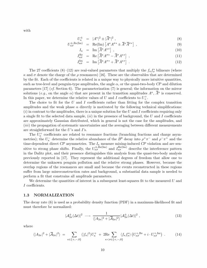
The 27 coefficients (8)–(12) are real-valued parameters that multiply the fκf∗σ bilinears (where

κ and σ denote the charge of the ρ resonances) [16]. These are the observables that are determinedby the fit. Each of the coefficients is related in a unique way to physically more intuitive quantities,such as tree-level and penguin-type amplitudes, the angle α, or the quasi-two-body CP and dilutionparameters [17] (cf. Section 6). The parameterization (7) is general; the information on the mirrorsolutions (e.g., on the angle α) that are present in the transition amplitudes Aκ, Aκ is conserved.In this paper, we determine the relative values of U and I coefficients to U+

+ .The choice to fit for the U and I coefficients rather than fitting for the complex transition

amplitudes and the weak phase α directly is motivated by the following technical simplifications:(i) in contrast to the amplitudes, there is a unique solution for the U and I coefficients requiring onlya single fit to the selected data sample, (ii) in the presence of background, the U and I coefficientsare approximately Gaussian distributed, which in general is not the case for the amplitudes, and(iii) the propagation of systematic uncertainties and the averaging between different measurementsare straightforward for the U ’s and I’s.

The U+κ coefficients are related to resonance fractions (branching fractions and charge asym-

metries); the U−κ determine the relative abundance of the B0 decay into ρ+π− and ρ−π+ and the

time-dependent direct CP asymmetries. The Iκ measure mixing-induced CP violation and are sen-sitive to strong phase shifts. Finally, the U±,Re(Im)

κσ and IRe(Im)κσ describe the interference pattern

in the Dalitz plot, and their presence distinguishes this analysis from the quasi-two-body analysispreviously reported in [17]. They represent the additional degrees of freedom that allow one todetermine the unknown penguin pollution and the relative strong phases. However, because theoverlap regions of the resonances are small and because the events reconstructed in these regionssuffer from large misreconstruction rates and background, a substantial data sample is needed toperform a fit that constrains all amplitude parameters.

We determine the quantities of interest in a subsequent least-squares fit to the measured U andI coefficients.

1.3 NORMALIZATION

The decay rate (6) is used as a probability density function (PDF) in a maximum-likelihood fit andmust therefore be normalized:

|A±3π(Δt)|2 −→ 1

〈|A3π|2 + |A3π|2〉|A±

3π(Δt)|2 , (13)

where

〈|A3π|2 + |A3π|2〉 =∑

κ∈{+,−,0}〈|fκ|2〉U+

κ + 2Re∑

κ<σ∈{+,−,0}〈fκf

∗σ〉

(U+,Re

κσ + i · U+,Imκσ

). (14)

10

The complex expectation values 〈fκf∗σ〉 are obtained from high-statistics Monte Carlo integration

of the Dalitz plot (3), taking into account acceptance and resolution effects.The normalization of the decay rate (6) renders the normalization of the U and I coefficients

arbitrary, so that we can fix one coefficient. By convention, we set U++ ≡ 1.

1.4 THE SQUARE DALITZ PLOT

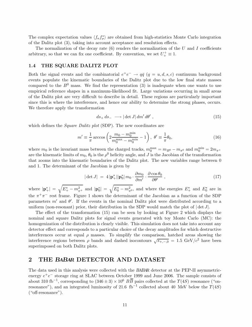
Both the signal events and the combinatorial e+e− → qq (q = u, d, s, c) continuum backgroundevents populate the kinematic boundaries of the Dalitz plot due to the low final state massescompared to the B0 mass. We find the representation (3) is inadequate when one wants to useempirical reference shapes in a maximum-likelihood fit. Large variations occurring in small areasof the Dalitz plot are very difficult to describe in detail. These regions are particularly importantsince this is where the interference, and hence our ability to determine the strong phases, occurs.We therefore apply the transformation

ds+ ds− −→ |det J | dm′ dθ′ , (15)

which defines the Square Dalitz plot (SDP). The new coordinates are

m′ ≡ 1π

arccos(

2m0 −mmin

0

mmax0 −mmin

0

− 1), θ′ ≡ 1

πθ0, (16)

where m0 is the invariant mass between the charged tracks, mmax0 = mB0 −mπ0 and mmin

0 = 2mπ+

are the kinematic limits ofm0, θ0 is the ρ0 helicity angle, and J is the Jacobian of the transformationthat zooms into the kinematic boundaries of the Dalitz plot. The new variables range between 0and 1. The determinant of the Jacobian is given by

|det J | = 4 |p∗+||p∗

0|m0 · ∂m0

∂m′ ·∂ cos θ0∂θ′

, (17)

where |p∗+| =

√E∗

+ −m2π+ and |p∗

0| =√E∗

0 −m2π0 , and where the energies E∗

+ and E∗0 are in

the π+π− rest frame. Figure 1 shows the determinant of the Jacobian as a function of the SDPparameters m′ and θ′. If the events in the nominal Dalitz plot were distributed according to auniform (non-resonant) prior, their distribution in the SDP would match the plot of |detJ |.

The effect of the transformation (15) can be seen by looking at Figure 2 which displays thenominal and square Dalitz plots for signal events generated with toy Monte Carlo (MC): thehomogenization of the distribution is clearly visible. This simulation does not take into account anydetector effect and corresponds to a particular choice of the decay amplitudes for which destructiveinterferences occur at equal ρ masses. To simplify the comparison, hatched areas showing theinterference regions between ρ bands and dashed isocontours √

s+,−,0 = 1.5 GeV/c2 have beensuperimposed on both Dalitz plots.

2 THE BABAR DETECTOR AND DATASET

The data used in this analysis were collected with the BABAR detector at the PEP-II asymmetric-energy e+e− storage ring at SLAC between October 1999 and June 2006. The sample consists ofabout 310 fb−1, corresponding to (346 ± 3)× 106 BB pairs collected at the Υ (4S) resonance (“on-resonance”), and an integrated luminosity of 21.6 fb−1 collected about 40 MeV below the Υ (4S)(“off-resonance”).

11

A detailed description of the BABAR detector is presented in Ref. [18]. The tracking system usedfor track and vertex reconstruction has two main components: a silicon vertex tracker (SVT) and adrift chamber (DCH), both operating within a 1.5 T magnetic field generated by a superconductingsolenoidal magnet. Photons are identified in an electromagnetic calorimeter (EMC) surroundinga detector of internally reflected Cherenkov light (DIRC), which associates Cherenkov photonswith tracks for particle identification (PID). Muon candidates are identified with the use of theinstrumented flux return (IFR) of the solenoid.

3 ANALYSIS METHOD

The U and I coefficients and the B0 → π+π−π0 event yield are determined by a maximum-likelihood fit of the signal model to the selected candidate events. Kinematic and event shapevariables exploiting the characteristic properties of the events are used in the fit to discriminatesignal from background.

3.1 EVENT SELECTION AND BACKGROUND SUPPRESSION

We reconstruct B0 → π+π−π0 candidates from pairs of oppositely-charged tracks, which are re-quired to form a good quality vertex, and a π0 candidate. In order to ensure that all events arewithin the Dalitz plot bounaries, we constrain the three-pion invariant mass to the B-mass. Weuse information from the tracking system, EMC, and DIRC to remove tracks for which the PIDis consistent with the electron, kaon, or proton hypotheses. In addition, we require that at leastone track has a signature in the IFR that is inconsistent with the muon hypothesis. The π0 can-didate mass must satisfy 0.11 < m(γγ) < 0.16GeV/c2, where each photon is required to have anenergy greater than 50MeV in the laboratory frame (LAB) and to exhibit a lateral profile of energydeposition in the EMC consistent with an electromagnetic shower.

A B-meson candidate is characterized kinematically by the energy-substituted mass mES =[(1

2s+ p0 · pB)2/E20 − p2

B ]12 and energy difference ΔE = E∗

B − 12

√s, where (EB ,pB) and (E0,p0)

are the four-vectors of the B-candidate and the initial electron-positron system, respectively. Theasterisk denotes the Υ (4S) frame, and s is the square of the invariant mass of the electron-positronsystem. We require 5.272 < mES < 5.288GeV/c2, which retains 81% of the signal and 8% of thecontinuum background events. The ΔE resolution exhibits a dependence on the π0 energy andtherefore varies across the Dalitz plot. We account for this effect by introducing the transformedquantity ΔE′ = (2ΔE−ΔE+−ΔE−)/(ΔE+−ΔE−), with ΔE±(m0) = c±−(c± ∓ c) (m0/m

max0 )2,

where m0 is strongly correlated with the energy of π0. We use the values c = 0.045GeV, c− =−0.140GeV, c+ = 0.080GeV, mmax

0 = 5.0GeV, and require −1 < ΔE′ < 1. These values havebeen obtained from Monte Carlo simulation and are tuned to maximize the selection of correctlyreconstructed over misreconstructed signal events. The requirement retains 75% (25%) of the signal(continuum).

Backgrounds arise primarily from random combinations in continuum events. To enhance dis-crimination between signal and continuum, we use a neural network (NN) [19] to combine fourdiscriminating variables: the angles with respect to the beam axis of the B momentum and Bthrust axis in the Υ (4S) frame, and the zeroth and second order monomials L0,2 of the energy flowabout the B thrust axis. The monomials are defined by Lj =

∑i pi × |cos θi|j, where θi is the

angle with respect to the B thrust axis of track or neutral cluster i, pi is its momentum, and thesum excludes the B candidate. The NN is trained in the signal region with off-resonance data and

12

simulated signal events. The final sample of signal candidates is selected with a requirement onthe NN output that retains 77% (8%) of the signal (continuum).

The time difference Δt is obtained from the measured distance between the z positions (alongthe beam direction) of the B0

3π and B0tag decay vertices, and the boost βγ = 0.56 of the e+e−

system: Δt = Δz/βγc. To determine the flavor of the B0tag we use the B flavor tagging algorithm

of Ref. [22]. This produces six mutually exclusive tagging categories. We also retain untaggedevents in a seventh category to improve the efficiency of the signal selection and because theseevents contribute to the measurement of direct CP violation. Events with multiple B candidatespassing the full selection occur in 16% (ρ±π∓) and 9% (ρ0π0) of the cases. If the multiple candidateshave different π0’s, we choose the candidate with the reconstructed π0 mass closest to the nominalone; in the case that both candidates have the same π0, we pick the first one.

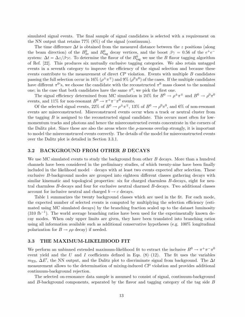
The signal efficiency determined from MC simulation is 24% for B0 → ρ±π∓ and B0 → ρ0π0

events, and 11% for non-resonant B0 → π+π−π0 events.Of the selected signal events, 22% of B0 → ρ±π∓, 13% of B0 → ρ0π0, and 6% of non-resonant

events are misreconstructed. Misreconstruced events occur when a track or neutral cluster fromthe tagging B is assigned to the reconstructed signal candidate. This occurs most often for low-momentum tracks and photons and hence the misreconstructed events concentrate in the corners ofthe Dalitz plot. Since these are also the areas where the ρ-mesons overlap strongly, it is importantto model the misreconstruced events correctly. The details of the model for misreconstructed eventsover the Dalitz plot is detailed in Section 3.3.1.

3.2 BACKGROUND FROM OTHER B DECAYS

We use MC simulated events to study the background from other B decays. More than a hundredchannels have been considered in the preliminary studies, of which twenty-nine have been finallyincluded in the likelihood model – decays with at least two events expected after selection. Theseexclusive B-background modes are grouped into eighteen different classes gathering decays withsimilar kinematic and topological properties: six for charged charmless B-decays, eight for neu-tral charmless B-decays and four for exclusive neutral charmed B-decays. Two additional classesaccount for inclusive neutral and charged b→ c decays.

Table 1 summarizes the twenty background classes which are used in the fit. For each mode,the expected number of selected events is computed by multiplying the selection efficiency (esti-mated using MC simulated decays) by the branching fraction scaled up to the dataset luminosity(310 fb−1). The world average branching ratios have been used for the experimentally known de-cay modes. When only upper limits are given, they have been translated into branching ratiosusing all information available such as additional conservative hypotheses (e.g. 100% longitudinalpolarization for B → ρρ decay) if needed.

3.3 THE MAXIMUM-LIKELIHOOD FIT

We perform an unbinned extended maximum-likelihood fit to extract the inclusive B0 → π+π−π0

event yield and the U and I coefficients defined in Eqs. (8)–(12). The fit uses the variablesmES, ΔE′, the NN output, and the Dalitz plot to discriminate signal from background. The Δtmeasurement allows to the determination of mixing-induced CP violation and provides additionalcontinuum-background rejection.

The selected on-resonance data sample is assumed to consist of signal, continuum-backgroundand B-background components, separated by the flavor and tagging category of the tag side B

13

decay. The signal likelihood consists of the sum of a correctly reconstructed (“truth-matched”,TM) component and a misreconstructed (“self-cross-feed”, SCF) component.

The probability density function (PDF) Pci for an event i in tagging category c is the sum of

the probability densities of all components, namely

Pci ≡ N3πf

c3π

[(1 − f

cSCF)Pc

3π−TM,i + fcSCFPc

3π−SCF,i

]

+ N cqq

12

(1 + qtag,iAqq, tag)Pcqq,i

+NB+

class∑j=1

NB+jfcB+j

12

(1 + qtag,iAB+, tag,j

)PcB+,ij

+NB0

class∑j=1

NB0jfcB0jPc

B0,ij , (18)

where: N3π is the total number of π+π−π0 signal events in the data sample; f c3π is the fraction

of signal events that are tagged in category c; f cSCF is the fraction of SCF events in tagging

category c, averaged over the Dalitz plot; Pc3π−TM,i and Pc

3π−SCF,i are the products of PDFs of thediscriminating variables used in tagging category c for TM and SCF events, respectively; N c

qq isthe number of continuum events that are tagged in category c; qtag,i is the tag flavor of the event,defined to be +1 for a B0

tag and −1 for a B0tag; Aqq, tag parameterizes possible tag asymmetry in

continuum events; Pcqq,i is the continuum PDF for tagging category c; NB+

class (NB0

class) is the numberof charged (neutral) B-related background classes considered in the fit; NB+j (NB0j) is the numberof expected events in the charged (neutral) B-background class j; f c

B+j (f cB0j) is the fraction of

charged (neutral) B-background events of class j that are tagged in category c; AB+, tag,j describesa possible tag asymmetry in the charged-B background class j; correlations between the tag andthe position in the Dalitz plot (the “charge”) are absorbed in tag-flavor-dependent Dalitz plotPDFs that are used for charged-B and continuum background; Pc

B+,ij is the B+-background PDFfor tagging category c and class j; finally, Pc

B0,ij is the neutral-B-background PDF for taggingcategory c and class j.

The PDFs PcX (X = {TM,SCF, continuum,B − bkg}) are the product of the four PDFs of the

discriminating variables, x1 = mES , x2 = ΔE′, x3 = NNoutput, and the triplet x4 = {m′, θ′,Δt}:

PcX,i(j) ≡

4∏k=1

P cX,i(j)(xk) . (19)

The extended likelihood over all tagging categories is given by

L ≡7∏

c=1

e−Nc

Nc∏i

Pci , (20)

where N c is the total number of events expected in category c.A total of 68 parameters, including the inclusive signal yield and the parameters from Eq. (6),

are varied in the fit. Most of the parameters describing the continuum distributions are also floatedin the fit.

14

3.3.1 THE Δt AND DALITZ PLOT PDFS

The Dalitz plot PDFs require as input the Dalitz plot-dependent relative selection efficiency, ε =ε(m′, θ′), and SCF fraction, fSCF = fSCF(m′, θ′). Both quantities are taken from MC simulation.Away from the Dalitz plot corners the efficiency is uniform, while it decreases when approaching thecorners, where one out of the three bodies in the final state is close to rest so that the acceptancerequirements on the particle reconstruction become restrictive. Combinatorial backgrounds andhence SCF fractions are large in the corners of the Dalitz plot due to the presence of soft neutralclusters and tracks.

For an event i, we define the time-dependent Dalitz plot PDFs

P3π−TM,i = εi (1 − fSCF,i) |det Ji| |A±3π(Δt)|2 , (21)

P3π−SCF, i = εi fSCF,i |det Ji| |A±3π(Δt)|2 , (22)

where P3π−TM,i and P3π−SCF, i are normalized. The corresponding phase space integration involvesthe expectation values 〈ε (1 − fSCF) |det J | fκfσ∗〉 and 〈ε fSCF |det J | fκfσ∗〉 for TM and SCFevents, where the indices κ, σ run over all resonances belonging to the signal model. The expectationvalues are model-dependent and are computed with the use of MC integration over the square Dalitzplot:

〈ε (1 − fSCF) |det J | fκfσ∗〉 =

∫ 10

∫ 10 ε (1 − fSCF) |det J | fκfσ∗ dm′dθ′∫ 1

0

∫ 10 ε |det J | fκfσ∗ dm′dθ′

, (23)

and similarly for 〈ε |det J | fκfσ∗〉, where all quantities in the integrands are Dalitz plot-dependent.Equation (18) invokes the phase space-averaged SCF fraction fSCF ≡ 〈fSCF |detJ | fκfσ∗〉. The

PDF normalization is decay-dynamics-dependent and is computed iteratively. We determine theaverage SCF fractions separately for each tagging category from MC simulation.

The width of the dominant ρ(770) resonance is large compared to the mass resolution for TMevents (about 8MeV/c2 core Gaussian resolution). We therefore neglect resolution effects in theTM model. Misreconstructed events have a poor mass resolution that strongly varies across theDalitz plot. It is described in the fit by a 2× 2-dimensional resolution function

RSCF(m′r, θ

′r,m

′t, θ

′t) , (24)

which represents the probability to reconstruct at the coordinate (m′r, θ

′r) an event that has the

true coordinate (m′t, θ

′t). It obeys the unitarity condition

1∫0

1∫0

RSCF(m′r, θ

′r,m

′t, θ

′t) dm

′rdθ

′r = 1, (25)

and is convolved with the signal model. The RSCF function is obtained from MC simulation.We use the signal model described in Section 1.1. It contains the dynamical information and

is connected with Δt via the matrix element (6), which serves as PDF. It is diluted by the effectsof mistagging and the limited vertex resolution [17]. The Δt resolution function for signal andB-background events is a sum of three Gaussian distributions, with parameters determined by afit to fully reconstructed B0 decays [22].

The Dalitz plot- and Δt-dependent PDFs factorize for the charged-B-background modes, but not(necessarily) for the neutral-B background due to B0B0 mixing.

15

The charged B-background contribution to the likelihood (18) involves the parameter AB+, tag,multiplied by the tag flavor qtag of the event. In the presence of significant tag-“charge” correla-tion (represented by an effective flavor-tag-versus-Dalitz-coordinate correlation), it parameterizespossible direct CP violation in these events. We also use distinct square Dalitz plot PDFs for eachreconstructed B flavor tag, and a flavor-tag-averaged PDF for untagged events. The PDFs areobtained from MC simulation and are described with the use of non-parametric functions. TheΔt resolution parameters are determined by a fit to fully reconstructed B+ decays. For each B+-background class we adjust effective lifetimes to account for the misreconstruction of the event thatmodifies the nominal Δt resolution function.

The neutral-B background is parameterized with PDFs that depend on the flavor tag of theevent. In the case of CP eigenstates, correlations between the flavor tag and the Dalitz coordinateare expected to be small. However, non-CP eigenstates, such as a±1 π

∓, may exhibit such correlation.Both types of decays can have direct and mixing-induced CP violation. A third type of decaysinvolves charged kaons and does not exhibit mixing-induced CP violation, but usually has a strongcorrelation between the flavor tag and the Dalitz plot coordinate (the kaon charge), because itconsists of B-flavor eigenstates. The Dalitz plot PDFs are obtained from MC simulation and aredescribed with the use of non-parametric functions. For neutral B background, the signal Δtresolution model is assumed.

The Dalitz plot treatment of the continuum events is similar to the one used for charged-Bbackground. The square Dalitz plot PDF for continuum background is obtained from on-resonanceevents selected in the mES sidebands and corrected for feed-through from B decays. A largenumber of cross checks has been performed to ensure the high fidelity of the empirical shapeparameterization. Analytical models have been found insufficient. The continuum Δt distributionis parameterized as the sum of three Gaussian distributions with common mean and three distinctwidths that scale the Δt per-event error. This yields six shape parameters that are determined bythe fit. The model is motivated by the observation that the Δt average is independent of its error,and that the Δt RMS depends linearly on the Δt error.

3.3.2 PARAMETERIZATION OF THE OTHER VARIABLES

The mES distribution of TM signal events is parameterized by a bifurcated Crystal Ball func-tion [21], which is a combination of a one-sided Gaussian and a Crystal Ball function. The meanof this function is determined by the fit. A non-parametric function is used to describe the SCFsignal component.

The ΔE′ distribution of TM events is parameterized by a double Gaussian function, whereall five parameters depend linearly on m2

0. Misreconstructed events are parameterized by a broadsingle Gaussian function.

Both mES and ΔE′ PDFs are parameterized by non-parametric functions for all B-backgroundclasses.

The mES and ΔE′ PDFs for continuum events are parameterized with an Argus shape func-tion [23] and a second order polynomial, respectively, with parameters determined by the fit.

We use non-parametric functions to empirically describe the distributions of the NN outputsfound in the MC simulation for TM and SCF signal events, and for B-background events. Wedistinguish tagging categories for TM signal events to account for differences observed in the shapes.

The continuum NN distribution is parameterized by a third order polynomial that is defined tobe positive. The coefficients of the polynomial are determined by the fit. Continuum events exhibita correlation between the Dalitz plot coordinate and the shape of the event that is exploited in the

16

NN. To correct for residual effects, we introduce a linear dependence of the polynomial coefficientson the distance of the Dalitz plot coordinate to the kinematic boundaries of the Dalitz plot. Theparameters describing this dependence are determined by the fit.

4 SYSTEMATIC STUDIES

The contributions to the systematic error on the signal parameters are summarized in Table 3.Table 4 summarizes the correlation coefficient extracted from the systematic covariance matrix.

The most important contribution to the systematic uncertainty stems from the signal modelingof the Dalitz plot dynamics.

To estimate the contribution to B0 → π+π−π0 decay via other resonances and non-resonantdecays, we have performed an independent analysis where we include these other decays in the fitmodel. For simplicity, we assume a uniform Dalitz distribution for the non-resonance events andconsider possible resonances including f0(980), f2(1270), and a low mass s-wave σ. The fit doesnot find significant number of any of those decays. However, the inclusion of a low mass π+π−

s-wave component degrades our ability to identify ρ0π0 events significantly. The systematic effects(contained in the “Dalitz plot model” field in Table 3) is estimated by observing the differencebetween the true values and Monte Carlo fit results, in which events are generated based on thenew fit results and fit with the nominal setup where only ρ is taken into account.

We vary the mass and width of the ρ(770), ρ(1450) and ρ(1700) within ranges that exceed twicethe errors found for these parameters in the fits to τ and e+e− data [11], and assign the observeddifferences in the measured U and I coefficients as systematic uncertainties (“ρ, ρ′, ρ′′ lineshape” inTable 3). Since some of the U and I coefficients exhibit significant dependence on the ρ(1450) andρ(1700) contributions, we leave their amplitudes (phases and fractions) free to vary in the nominalfit.

To validate the fitting tool, we perform fits on large MC samples with the measured proportionsof signal, continuum and B-background events. No significant biases are observed in these fits. Thestatistical uncertainties on the fit parameters are taken as systematic uncertainties (“Fit bias” inTable 3).

Another major source of systematic uncertainty is the B-background model. The expectedevent yields from the background modes are varied according to the uncertainties in the measuredor estimated branching fractions (“NBackground” in Table 3). SinceB-background modes may exhibitCP violation, the corresponding parameters are varied within appropriate uncertainty ranges (“Bbackground CP” in Table 3). As is done for the signal PDFs, we vary the Δt resolution parametersand the flavor-tagging parameters within their uncertainties and assign the differences observed inthe on-resonance data fit with respect to nominal fit as systematic errors.

Other systematic effects are much less important to the measurements of U and I coefficients,and they are combined in “Others” field in Table 3. Details are given below.

The parameters for the continuum events are determined by the fit. No additional systematicuncertainties are assigned to them. An exception to this is the Dalitz plot PDF: to estimatethe systematic uncertainty from the mES sideband extrapolation, we select large samples of off-resonance data by loosening the requirements on ΔE and the NN. We compare the distributionsof m′ and θ′ between the mES sideband and the signal region. No significant differences are found.We assign as systematic error the effect seen when weighting the continuum Dalitz plot PDF bythe ratio of both data sets. This effect is mostly statistical in origin.

17

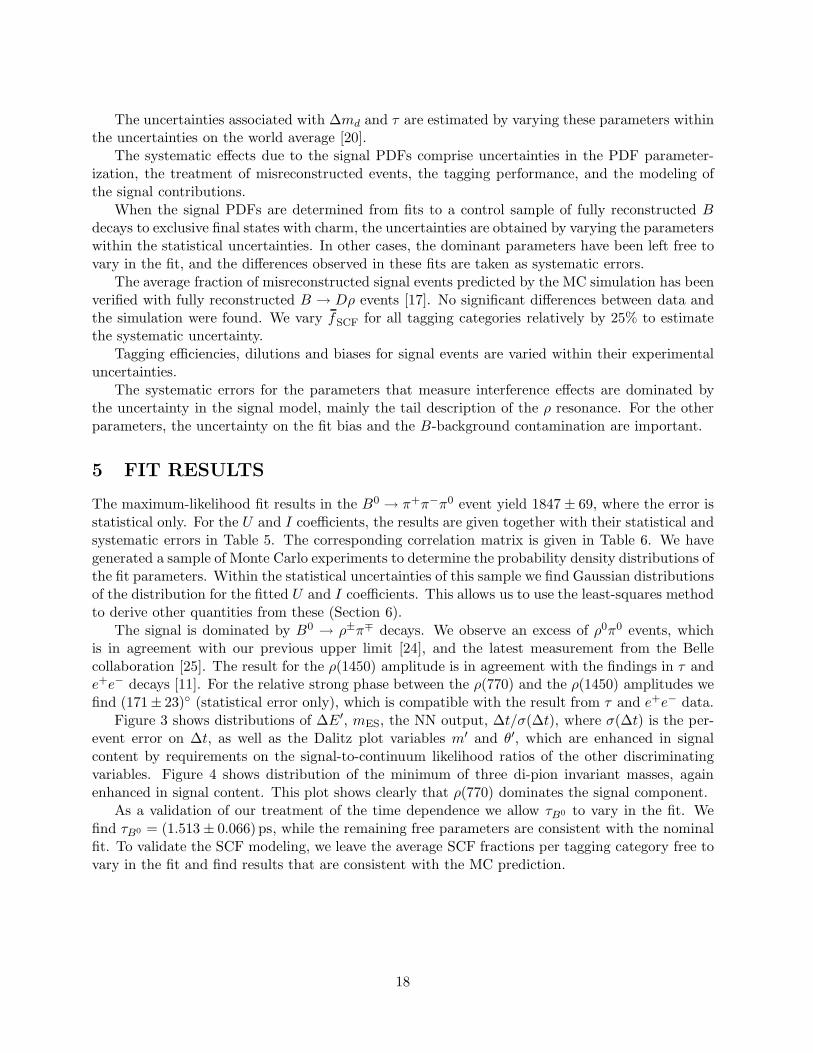
The uncertainties associated with Δmd and τ are estimated by varying these parameters withinthe uncertainties on the world average [20].

The systematic effects due to the signal PDFs comprise uncertainties in the PDF parameter-ization, the treatment of misreconstructed events, the tagging performance, and the modeling ofthe signal contributions.

When the signal PDFs are determined from fits to a control sample of fully reconstructed Bdecays to exclusive final states with charm, the uncertainties are obtained by varying the parameterswithin the statistical uncertainties. In other cases, the dominant parameters have been left free tovary in the fit, and the differences observed in these fits are taken as systematic errors.

The average fraction of misreconstructed signal events predicted by the MC simulation has beenverified with fully reconstructed B → Dρ events [17]. No significant differences between data andthe simulation were found. We vary fSCF for all tagging categories relatively by 25% to estimatethe systematic uncertainty.

Tagging efficiencies, dilutions and biases for signal events are varied within their experimentaluncertainties.

The systematic errors for the parameters that measure interference effects are dominated bythe uncertainty in the signal model, mainly the tail description of the ρ resonance. For the otherparameters, the uncertainty on the fit bias and the B-background contamination are important.

5 FIT RESULTS

The maximum-likelihood fit results in the B0 → π+π−π0 event yield 1847 ± 69, where the error isstatistical only. For the U and I coefficients, the results are given together with their statistical andsystematic errors in Table 5. The corresponding correlation matrix is given in Table 6. We havegenerated a sample of Monte Carlo experiments to determine the probability density distributions ofthe fit parameters. Within the statistical uncertainties of this sample we find Gaussian distributionsof the distribution for the fitted U and I coefficients. This allows us to use the least-squares methodto derive other quantities from these (Section 6).

The signal is dominated by B0 → ρ±π∓ decays. We observe an excess of ρ0π0 events, whichis in agreement with our previous upper limit [24], and the latest measurement from the Bellecollaboration [25]. The result for the ρ(1450) amplitude is in agreement with the findings in τ ande+e− decays [11]. For the relative strong phase between the ρ(770) and the ρ(1450) amplitudes wefind (171± 23)◦ (statistical error only), which is compatible with the result from τ and e+e− data.

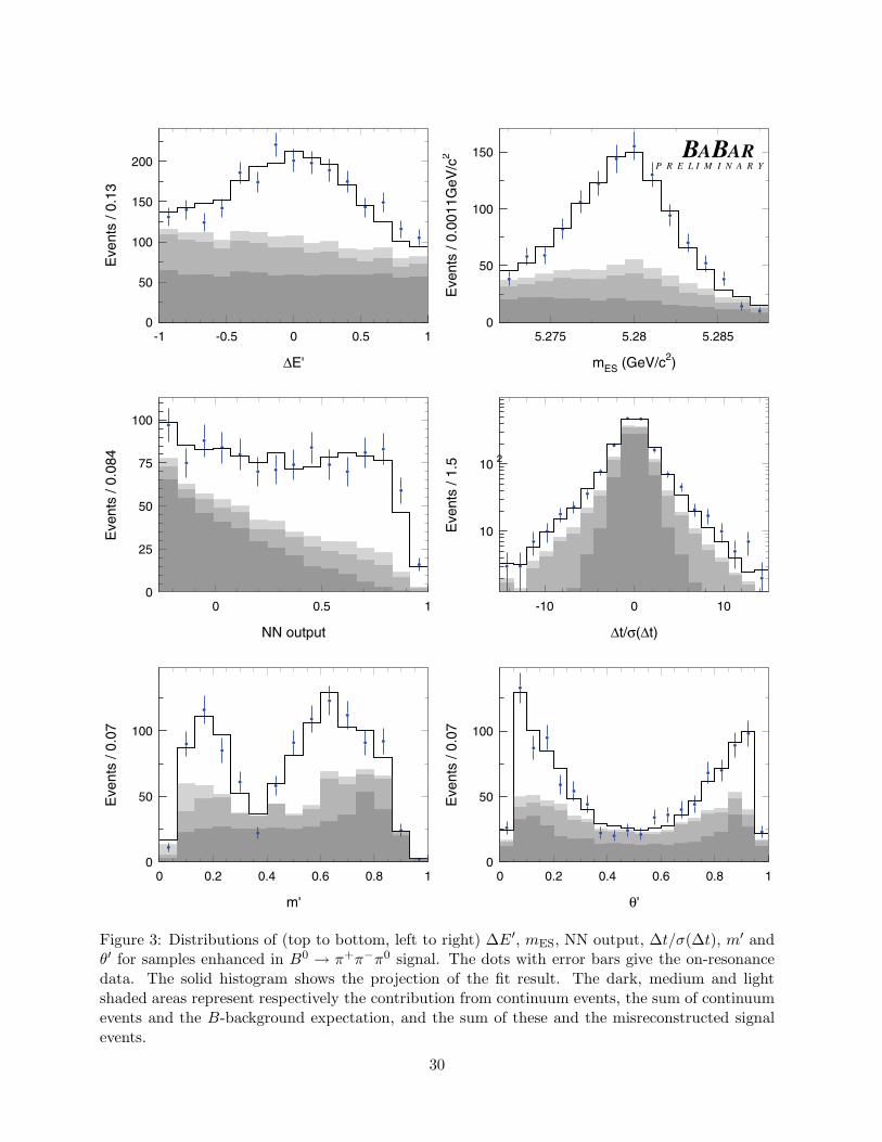
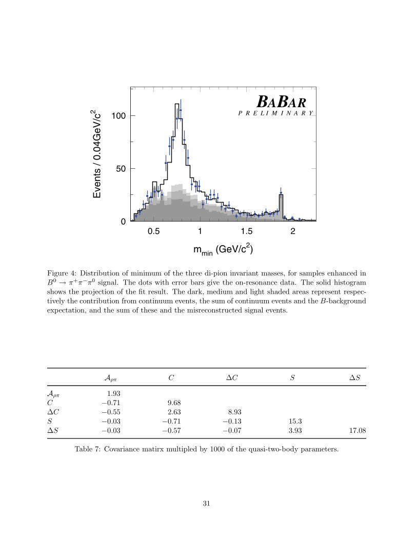
Figure 3 shows distributions of ΔE′, mES, the NN output, Δt/σ(Δt), where σ(Δt) is the per-event error on Δt, as well as the Dalitz plot variables m′ and θ′, which are enhanced in signalcontent by requirements on the signal-to-continuum likelihood ratios of the other discriminatingvariables. Figure 4 shows distribution of the minimum of three di-pion invariant masses, againenhanced in signal content. This plot shows clearly that ρ(770) dominates the signal component.

As a validation of our treatment of the time dependence we allow τB0 to vary in the fit. Wefind τB0 = (1.513 ± 0.066) ps, while the remaining free parameters are consistent with the nominalfit. To validate the SCF modeling, we leave the average SCF fractions per tagging category free tovary in the fit and find results that are consistent with the MC prediction.

18

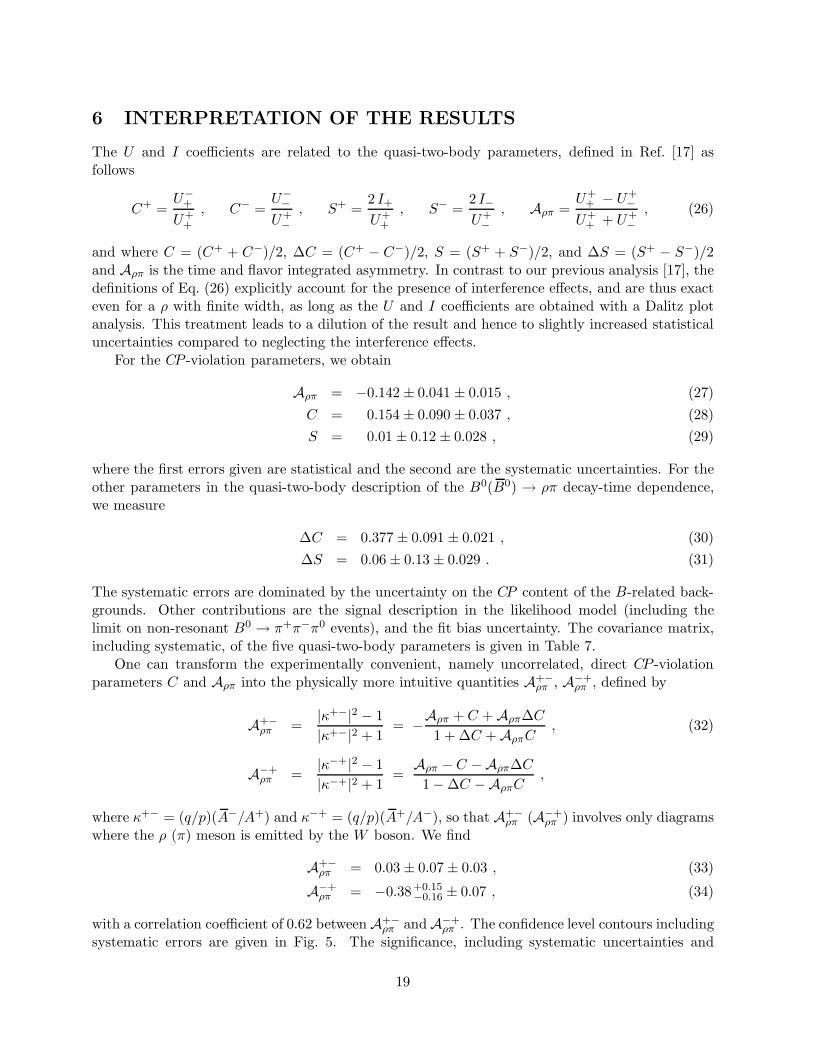
6 INTERPRETATION OF THE RESULTS

The U and I coefficients are related to the quasi-two-body parameters, defined in Ref. [17] asfollows

C+ =U−

+

U++

, C− =U−−

U+−, S+ =

2 I+U+

+

, S− =2 I−U+−

, Aρπ =U+

+ − U+−

U++ + U+

−, (26)

and where C = (C+ + C−)/2, ΔC = (C+ − C−)/2, S = (S+ + S−)/2, and ΔS = (S+ − S−)/2and Aρπ is the time and flavor integrated asymmetry. In contrast to our previous analysis [17], thedefinitions of Eq. (26) explicitly account for the presence of interference effects, and are thus exacteven for a ρ with finite width, as long as the U and I coefficients are obtained with a Dalitz plotanalysis. This treatment leads to a dilution of the result and hence to slightly increased statisticaluncertainties compared to neglecting the interference effects.

For the CP -violation parameters, we obtain

Aρπ = −0.142 ± 0.041 ± 0.015 , (27)C = 0.154 ± 0.090 ± 0.037 , (28)S = 0.01 ± 0.12 ± 0.028 , (29)

where the first errors given are statistical and the second are the systematic uncertainties. For theother parameters in the quasi-two-body description of the B0(B0) → ρπ decay-time dependence,we measure

ΔC = 0.377 ± 0.091 ± 0.021 , (30)ΔS = 0.06 ± 0.13 ± 0.029 . (31)

The systematic errors are dominated by the uncertainty on the CP content of the B-related back-grounds. Other contributions are the signal description in the likelihood model (including thelimit on non-resonant B0 → π+π−π0 events), and the fit bias uncertainty. The covariance matrix,including systematic, of the five quasi-two-body parameters is given in Table 7.

One can transform the experimentally convenient, namely uncorrelated, direct CP -violationparameters C and Aρπ into the physically more intuitive quantities A+−

ρπ , A−+ρπ , defined by

A+−ρπ =

|κ+−|2 − 1|κ+−|2 + 1

= −Aρπ + C + AρπΔC1 + ΔC + AρπC

, (32)

A−+ρπ =

|κ−+|2 − 1|κ−+|2 + 1

=Aρπ −C −AρπΔC1 − ΔC −AρπC

,

where κ+− = (q/p)(A−/A+) and κ−+ = (q/p)(A+/A−), so that A+−ρπ (A−+

ρπ ) involves only diagramswhere the ρ (π) meson is emitted by the W boson. We find

A+−ρπ = 0.03 ± 0.07 ± 0.03 , (33)

A−+ρπ = −0.38+0.15

−0.16 ± 0.07 , (34)

with a correlation coefficient of 0.62 between A+−ρπ and A−+

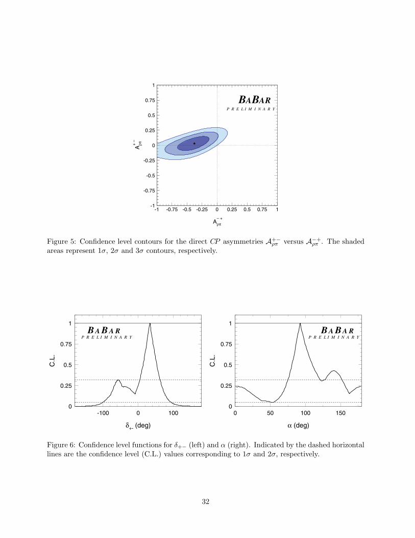
ρπ . The confidence level contours includingsystematic errors are given in Fig. 5. The significance, including systematic uncertainties and

19

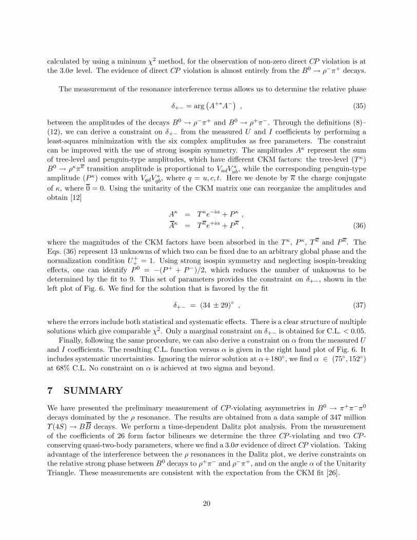
calculated by using a mininum χ2 method, for the observation of non-zero direct CP violation is atthe 3.0σ level. The evidence of direct CP violation is almost entirely from the B0 → ρ−π+ decays.

The measurement of the resonance interference terms allows us to determine the relative phase

δ+− = arg(A+∗A−)

, (35)

between the amplitudes of the decays B0 → ρ−π+ and B0 → ρ+π−. Through the definitions (8)–(12), we can derive a constraint on δ+− from the measured U and I coefficients by performing aleast-squares minimization with the six complex amplitudes as free parameters. The constraintcan be improved with the use of strong isospin symmetry. The amplitudes Aκ represent the sumof tree-level and penguin-type amplitudes, which have different CKM factors: the tree-level (T κ)B0 → ρκπκ transition amplitude is proportional to VudV

∗ub, while the corresponding penguin-type

amplitude (P κ) comes with VqdV∗qb, where q = u, c, t. Here we denote by κ the charge conjugate

of κ, where 0 = 0. Using the unitarity of the CKM matrix one can reorganize the amplitudes andobtain [12]

Aκ = T κe−iα + P κ ,

Aκ = T κe+iα + P κ , (36)

where the magnitudes of the CKM factors have been absorbed in the T κ, P κ, T κ and P κ. TheEqs. (36) represent 13 unknowns of which two can be fixed due to an arbitrary global phase and thenormalization condition U+

+ = 1. Using strong isospin symmetry and neglecting isospin-breakingeffects, one can identify P 0 = −(P+ + P−)/2, which reduces the number of unknowns to bedetermined by the fit to 9. This set of parameters provides the constraint on δ+−, shown in theleft plot of Fig. 6. We find for the solution that is favored by the fit

δ+− = (34 ± 29)◦ , (37)

where the errors include both statistical and systematic effects. There is a clear structure of multiplesolutions which give comparable χ2. Only a marginal constraint on δ+− is obtained for C.L. < 0.05.

Finally, following the same procedure, we can also derive a constraint on α from the measured Uand I coefficients. The resulting C.L. function versus α is given in the right hand plot of Fig. 6. Itincludes systematic uncertainties. Ignoring the mirror solution at α+180◦, we find α ∈ (75◦, 152◦)at 68% C.L. No constraint on α is achieved at two sigma and beyond.

7 SUMMARY

We have presented the preliminary measurement of CP -violating asymmetries in B0 → π+π−π0

decays dominated by the ρ resonance. The results are obtained from a data sample of 347 millionΥ (4S) → BB decays. We perform a time-dependent Dalitz plot analysis. From the measurementof the coefficients of 26 form factor bilinears we determine the three CP -violating and two CP -conserving quasi-two-body parameters, where we find a 3.0σ evidence of direct CP violation. Takingadvantage of the interference between the ρ resonances in the Dalitz plot, we derive constraints onthe relative strong phase between B0 decays to ρ+π− and ρ−π+, and on the angle α of the UnitarityTriangle. These measurements are consistent with the expectation from the CKM fit [26].

20

8 Acknowledgments

We are grateful for the extraordinary contributions of our PEP-II colleagues in achieving theexcellent luminosity and machine conditions that have made this work possible. The success ofthis project also relies critically on the expertise and dedication of the computing organizationsthat support BABAR. The collaborating institutions wish to thank SLAC for its support and thekind hospitality extended to them. This work is supported by the US Department of Energy andNational Science Foundation, the Natural Sciences and Engineering Research Council (Canada),Institute of High Energy Physics (China), the Commissariat a l’Energie Atomique and InstitutNational de Physique Nucleaire et de Physique des Particules (France), the Bundesministerium furBildung und Forschung and Deutsche Forschungsgemeinschaft (Germany), the Istituto Nazionaledi Fisica Nucleare (Italy), the Foundation for Fundamental Research on Matter (The Netherlands),the Research Council of Norway, the Ministry of Science and Technology of the Russian Federation,Ministerio de Educacion y Ciencia (Spain), and the Particle Physics and Astronomy ResearchCouncil (United Kingdom). Individuals have received support from the Marie-Curie IEF program(European Union) and the A. P. Sloan Foundation.

References

[1] BABAR Collaboration (B. Aubert et al.), Phys. Rev. Lett. 89, 201802 (2002).

[2] Belle Collaboration (K. Abe et al.), Phys. Rev. D 66, 071102 (2002).

[3] N. Cabibbo, Phys. Rev. Lett. 10, 531 (1963); M. Kobayashi and T. Maskawa, Prog. Theor.Phys. 49, 652 (1973).

[4] BABAR Collaboration, B. Aubert et al., Phys. Rev. Lett. 89, 281802 (2002); A. Jawahery, Int.J. Mod. Phys. A 19, 975 (2004)

[5] Belle Collaboration (K. Abe et al.), Phys. Rev. Lett. 93, 021601 (2004).

[6] BABAR Collaboration (B. Aubert et al.), Phys. Rev. Lett. 93, 231801 (2004).

[7] Belle Collaboration (K. Abe et al.), Phys. Rev. Lett. 96, 171801 (2006).

[8] M. Gronau and D. London, Phys. Rev. Lett. 65, 3381 (1990).

[9] H.J. Lipkin, Y. Nir, H.R. Quinn and A. Snyder, Phys. Rev. D44, 1454 (1991).

[10] H.R. Quinn and A.E. Snyder, Phys. Rev. D48, 2139 (1993).

[11] ALEPH Collaboration, (R. Barate et al.), Z. Phys. C76, 15 (1997); we use updated lineshapefits including new data from e+e− annihilation [13] and τ spectral functions [14] (masses andwidths in MeV/c2): mρ±(770) = 775.5 ± 0.6, mρ0(770) = 773.1 ± 0.5, Γρ±(770) = 148.2 ± 0.8,Γρ±(770) = 148.0 ± 0.9, mρ(1450) = 1409 ± 12, Γρ(1450) = 500 ± 37, mρ(1700) = 1749 ± 20, andΓρ(1700) ≡ 235.

[12] The BABAR Physics Book, Editors P.F. Harrison and H.R. Quinn, SLAC-R-504 (1998).

[13] R.R. Akhmetshin et al. (CMD-2 Collaboration), Phys. Lett. B527, 161 (2002).

21

[14] ALEPH Collaboration, ALEPH 2002-030 CONF 2002-019, (July 2002).

[15] G.J. Gounaris and J.J. Sakurai, Phys. Rev. Lett. 21, 244 (1968).

[16] H.R. Quinn and J. Silva, Phys. Rev. D62, 054002 (2000).

[17] BABAR Collaboration (B. Aubert et al.), Phys. Rev. Lett. 91, 201802 (2003); updated prelim-inary results at BABAR-PLOT-0055 (2003).

[18] BABAR Collaboration, B. Aubert et al., Nucl. Instrum. Methods A479, 1 (2002).

[19] P. Gay, B. Michel, J. Proriol, and O. Deschamps, “Tagging Higgs Bosons in Hadronic LEP-2Events with Neural Networks.”, In Pisa 1995, New computing techniques in physics research,725 (1995).

[20] Particle Data Group (S. Eidelman et al.), Phys. Lett. B592, 1 (2004).

[21] T. Skwarnicki, DESY F31-86-02, Ph.D. thesis (1986); see also Ref. [22].

[22] BABAR Collaboration, B. Aubert et al., Phys. Rev. D66, 032003 (2002).

[23] ARGUS Collaboration (H. Albrecht et al.), Z. Phys. C 48, 543 (1990; see also Ref. [22]).

[24] BABAR Collaboration (B. Aubert et al.), Phys. Rev. Lett. 93, 051802 (2004).

[25] Belle Collaboration (J. Dragic et al.), Phys. Rev. D73, 111105 (2006).

[26] J. Charles et al., Eur. Phys. J. C41, 1 (2005).

22

00.2

0.40.6

0.81

00.2

0.40.6

0.81

100

200

300

400

00.2

0.40.6

0.81

00.2

0.40.6

0.81

100

200

300

400

θ'

m'

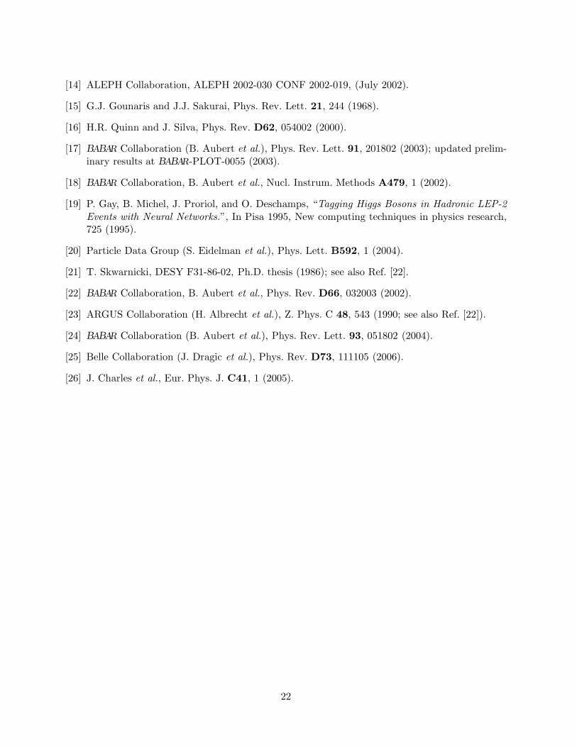
Figure 1: Jacobian determinant (17) of the transformation (15) defining the SDP. Such patternwould be obtained in the SDP if events were uniformly distributed over the nominal Dalitz plot.

0

5

10

15

20

25

30

0 5 10 15 20 25 30

s+ (GeV2/c4)

s –

(G

eV2 /c

4 )

0

1

2

3

4

5

22 23 24 25 26 27

Interference

√s0 = 1.5 GeV/c 2

√s+

= 1.

5 G

eV/c

2

√s– = 1.5 GeV/c2

0

0.2

0.4

0.6

0.8

1

0 0.2 0.4 0.6 0.8 1

m'

θ'

Interference

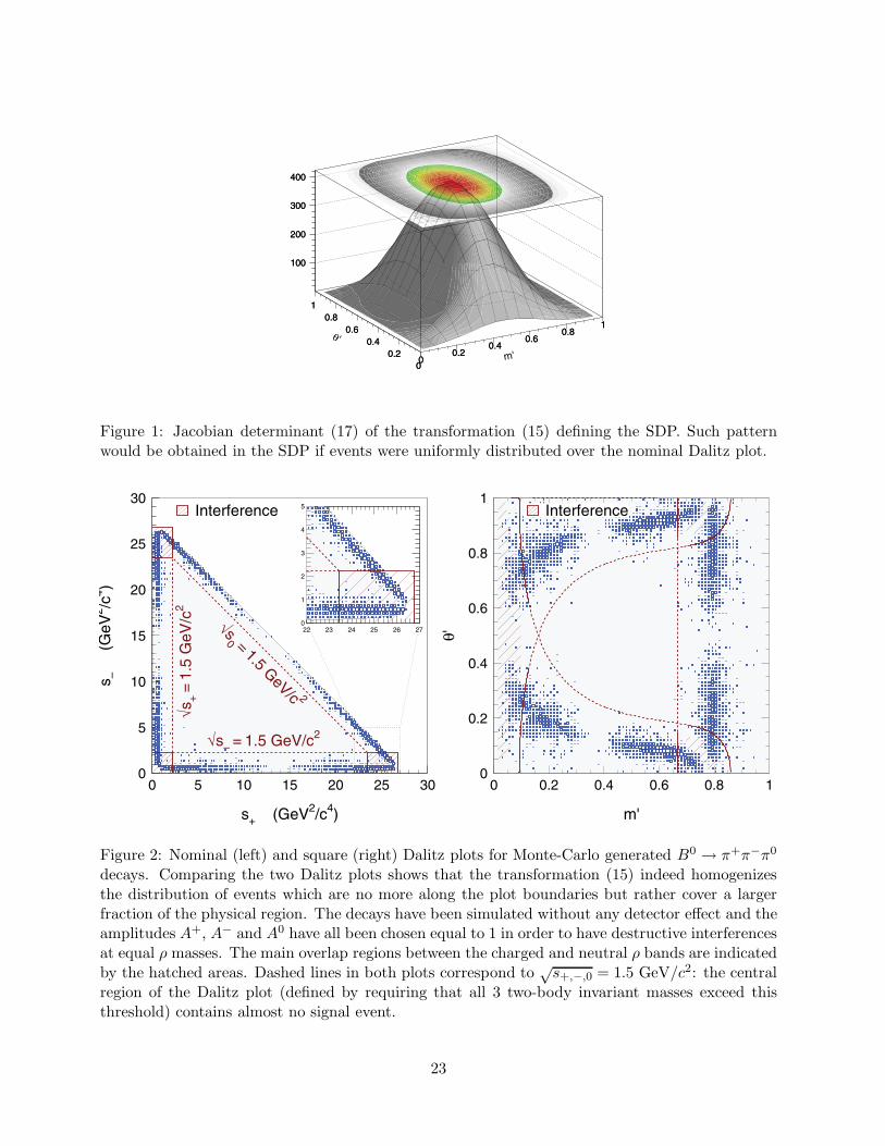
Figure 2: Nominal (left) and square (right) Dalitz plots for Monte-Carlo generated B0 → π+π−π0

decays. Comparing the two Dalitz plots shows that the transformation (15) indeed homogenizesthe distribution of events which are no more along the plot boundaries but rather cover a largerfraction of the physical region. The decays have been simulated without any detector effect and theamplitudes A+, A− and A0 have all been chosen equal to 1 in order to have destructive interferencesat equal ρ masses. The main overlap regions between the charged and neutral ρ bands are indicatedby the hatched areas. Dashed lines in both plots correspond to √

s+,−,0 = 1.5 GeV/c2: the centralregion of the Dalitz plot (defined by requiring that all 3 two-body invariant masses exceed thisthreshold) contains almost no signal event.

23

Class Mode BR [10−6] Expected number of events

0 B+ → ρ+ρ0[long] 19.1 ± 3.5 52 ± 10

0 B+ → a+1 (→ (ρπ)+)π0 20.0 ± 15.0 32 ± 24

0 B+ → a01(→ ρ+−π−+)π+ 20.0 ± 15.0 19 ± 14

1 B+ → π+ρ0 8.7 ± 1.0 73 ± 81 B+ → ρ0K+ 4.3 ± 0.6 6 ± 12 B+ → π+K0

S(→ π+π−) 8.3 ± 0.4 10 ± 13 B+ → π0ρ+ 10.8 ± 1.4 63 ± 83 B+ → π+K0

S(→ π0π0) 3.7 ± 0.2 15 ± 24 B+ → π+π0 5.5 ± 0.6 14 ± 24 B+ → K+π0 12.1 ± 0.8 8 ± 15 B+ → (K(∗∗)(1430)π)+ → (K+ππ)+ 29.0 ± 5.4 38 ± 56 B0 → π−K�+(→ K0

Sπ+) 3.3 ± 0.4 2 ± 1

7 B0 → ρ+ρ−[long]

25.2 ± 3.7 67 ± 107 B0 → (a1π)0 39.7 ± 3.7 39 ± 48 B0 → K+π− 18.9 ± 0.7 12 ± 09 B0 → π−K�+(→ K+π0) 3.3 ± 0.4 20 ± 29 B0 → K(∗∗)(1430)π → Kππ0 11.2 ± 2.2 212 ± 3410 B0 → γK�0(892, 1430)(→ (K+π−)0) 27.4 ± 1.5 14 ± 110 B0 → π0K�0(→ K+π−) 1.3 ± 0.5 9 ± 410 B0 → η′(→ ρ0γ)π0 0.4 ± 0.2 3 ± 211 B0 → ρ−K+ 9.9 ± 1.6 103 ± 1712 B0 → K+π−π0

[nonres] 4.6 ± 4.6 38 ± 3813 B0 → π0K0

S(→ π+π−) 5.8 ± 0.5 50 ± 414 B0 → D−(→ π−π0)π+ 7.5 ± 2.3 599 ± 18415 B0 → D0(→ K+π−)π0 11.0 ± 3.2 100 ± 2916 B0 → D0(→ π+π−)π0 0.4 ± 0.1 35 ± 917 B0 → J/ψ(→ e+e−, μ+μ−)π0 2.6 ± 0.5 77 ± 1518 B0 → {neutral generic b→ c decays} − 173 ± 1519 B+ → {charged generic b→ c decays} − 396 ± 20

Table 1: Summary of the B-background modes taken into account for the likelihood model. Theyhave been grouped in twenty classes: charged charmless (six), neutral charmless (eight), exclusiveneutral charmed (four) and inclusive neutral and charged charmed decays. Modes with at leasttwo events expected after final selection have been included.

24

Variable TM Signal SCF Signal Continuum B-Background

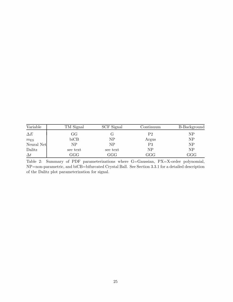
ΔE GG G P2 NPmES biCB NP Argus NPNeural Net NP NP P3 NPDalitz see text see text NP NPΔt GGG GGG GGG GGG

Table 2: Summary of PDF parameterizations where G=Gaussian, PX=X-order polynomial,NP=non-parametric, and biCB=bifurcated Crystal Ball. See Section 3.3.1 for a detailed descriptionof the Dalitz plot parameterization for signal.

25

I0 I− IIm−0 IRe

−0 I+ IIm+0

Dalitz plot model 0.010 0.006 0.110 0.102 0.020 0.018ρ,ρ′,ρ′′ lineshape 0.003 0.012 0.240 0.103 0.009 0.225Fit bias 0.014 0.023 0.173 0.375 0.008 0.186NBackground 0.002 0.008 0.064 0.085 0.005 0.026B background CP 0.005 0.009 0.082 0.061 0.011 0.039Others 0.002 0.006 0.104 0.052 0.005 0.051

Sum 0.017 0.027 0.315 0.402 0.023 0.292

IRe+0 IIm

+− IRe+− U−

0 U+0 U−,Im

−0 U−,Re−0

Dalitz plot model 0.017 0.007 0.127 0.082 0.041 0.144 0.209ρ,ρ′,ρ′′ lineshape 0.308 0.138 0.306 0.012 0.012 0.086 0.159Fit bias 0.301 0.036 0.048 0.088 0.001 0.050 0.087NBackground 0.049 0.178 0.176 0.002 0.009 0.034 0.045B background CP 0.042 0.044 0.095 0.015 0.002 0.020 0.073Others 0.073 0.059 0.095 0.004 0.002 0.012 0.050

Sum 0.431 0.143 0.335 0.121 0.043 0.175 0.276

U+,Im−0 U+,Re

−0 U−− U+

− U−,Im+0 U−,Re

+0 U+,Im+0

Dalitz plot model 0.034 0.024 0.022 0.030 0.036 0.258 0.076ρ,ρ′,ρ′′ lineshape 0.222 0.045 0.010 0.030 0.050 0.216 0.089Fit bias 0.034 0.058 0.004 0.005 0.053 0.007 0.004NBackground 0.045 0.017 0.013 0.005 0.117 0.103 0.034B background CP 0.032 0.018 0.032 0.009 0.063 0.075 0.019Others 0.027 0.015 0.010 0.002 0.045 0.020 0.027

Sum 0.227 0.078 0.025 0.043 0.082 0.337 0.117

U+,Re+0 U−,Im

+− U−,Re+− U+,Im

+− U+,Re+− U−

+

Dalitz plot model 0.045 0.014 0.250 0.703 0.227 0.010ρ,ρ′,ρ′′ lineshape 0.140 0.169 0.200 0.169 0.159 0.031Fit bias 0.020 0.007 0.069 0.012 0.033 0.027NBackground 0.069 0.137 0.122 0.024 0.166 0.014B background CP 0.014 0.042 0.029 0.025 0.025 0.034Others 0.024 0.032 0.067 0.024 0.044 0.009

Sum 0.148 0.170 0.328 0.723 0.279 0.042

Aρπ C ΔC S ΔS

Dalitz plot model 0.008 0.002 0.013 0.015 0.024ρ,ρ′,ρ′′ lineshape 0.011 0.021 0.011 0.016 0.008Fit bias 0.004 0.012 0.015 0.028 0.011NBackground 0.002 0.005 0.011 0.002 0.011B background CP 0.003 0.029 0.006 0.017 0.005Others 0.001 0.007 0.005 0.006 0.007

Sum 0.015 0.037 0.021 0.028 0.029

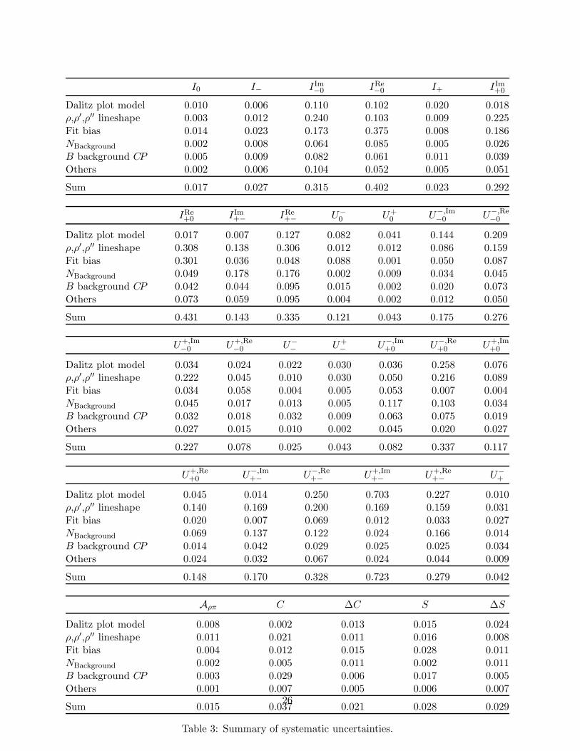
Table 3: Summary of systematic uncertainties.

26

N3π I0 I− IIm−0 IRe

−0 I+ IIm+0 IRe

+0 IIm+− IRe

+− U−0 U+

0 U−,Im−0

N3π 1.00I0 0.15 1.00I− 0.52 0.47 1.00IIm−0 −0.24 −0.01 0.05 1.00IRe−0 −0.64 0.28 −0.41 −0.08 1.00I+ −0.26 0.37 0.26 −0.35 0.43 1.00IIm+0 −0.23 0.17 −0.26 −0.22 0.56 0.33 1.00IRe+0 −0.29 −0.02 0.02 0.65 −0.08 −0.21 −0.48 1.00IIm+− 0.84 0.13 0.39 −0.39 −0.57 −0.24 −0.13 −0.45 1.00IRe+− 0.40 −0.23 0.23 0.39 −0.63 −0.66 −0.42 0.36 0.35 1.00U−

0 0.00 0.47 0.04 0.02 0.13 0.06 0.31 −0.03 0.05 −0.04 1.00U+

0 0.11 −0.22 0.12 0.31 −0.27 −0.21 −0.21 0.24 −0.05 0.44 −0.14 1.00U−,Im−0 −0.66 0.10 −0.44 −0.02 0.75 0.48 0.31 −0.03 −0.63 −0.69 −0.07 −0.15 1.00

U−,Re−0 0.27 −0.17 −0.06 −0.69 −0.15 0.10 −0.19 −0.31 0.36 −0.02 −0.40 −0.11 −0.19

U+,Im−0 0.24 0.56 0.05 −0.61 0.26 0.31 0.31 −0.51 0.38 −0.49 0.28 −0.52 0.03

U+,Re−0 0.25 0.01 −0.01 −0.40 −0.05 −0.01 −0.13 −0.25 0.33 −0.10 −0.37 −0.30 −0.06

U−− 0.25 0.24 0.12 −0.05 −0.16 0.05 0.07 −0.09 0.27 0.04 0.42 −0.14 0.06

U+− −0.39 0.12 −0.16 −0.02 0.24 0.25 0.21 0.00 −0.29 −0.26 0.21 −0.02 0.19

U−,Im+0 0.66 0.12 0.27 −0.55 −0.42 −0.04 −0.03 −0.63 0.76 −0.07 −0.05 −0.20 −0.26

U−,Re+0 0.66 −0.10 0.28 −0.38 −0.66 −0.24 −0.47 −0.27 0.72 0.31 −0.31 0.10 −0.47

U+,Im+0 −0.48 0.24 −0.34 −0.31 0.78 0.54 0.68 −0.36 −0.39 −0.83 0.21 −0.45 0.68

U+,Re+0 0.76 0.21 0.35 −0.41 −0.45 −0.16 −0.03 −0.54 0.83 0.08 0.09 −0.24 −0.52

U−,Im+− −0.71 −0.19 −0.34 0.51 0.50 0.07 0.22 0.40 −0.78 −0.11 0.09 0.10 0.50

U−,Re+− −0.78 −0.15 −0.41 0.36 0.50 0.13 0.04 0.46 −0.90 −0.23 −0.01 0.13 0.58

U+,Im+− −0.35 −0.07 −0.25 0.36 0.25 −0.12 0.14 0.29 −0.33 −0.02 0.06 0.01 0.25

U+,Re+− −0.78 −0.20 −0.37 0.45 0.57 0.17 0.22 0.40 −0.85 −0.18 0.03 0.13 0.57

U−+ −0.14 0.10 −0.01 0.05 0.00 0.01 0.07 −0.03 0.02 0.03 0.37 0.03 0.21

U−,Re−0 U+,Im

−0 U+,Re−0 U−

− U+− U−,Im

+0 U−,Re+0 U+,Im

+0 U+,Re+0 U−,Im

+− U−,Re+− U+,Im

+− U+,Re+− U−

+

U−,Re−0 1.00

U+,Im−0 0.39 1.00

U+,Re−0 0.60 0.43 1.00

U−− −0.26 0.12 −0.13 1.00

U+− −0.07 0.21 −0.37 −0.14 1.00

U−,Im+0 0.35 0.52 0.43 0.30 −0.20 1.00

U−,Re+0 0.61 0.21 0.43 0.08 −0.22 0.76 1.00

U+,Im+0 −0.11 0.47 0.04 −0.00 0.30 −0.08 −0.49 1.00

U+,Re+0 0.30 0.56 0.47 0.17 −0.27 0.77 0.56 −0.11 1.00

U−,Im+− −0.59 −0.59 −0.53 −0.13 0.10 −0.80 −0.82 0.30 −0.75 1.00

U−,Re+− −0.33 −0.41 −0.41 −0.31 0.32 −0.73 −0.63 0.25 −0.83 0.69 1.00

U+,Im+− −0.44 −0.25 −0.44 0.05 0.10 −0.33 −0.42 0.15 −0.35 0.49 0.34 1.00

U+,Re+− −0.50 −0.56 −0.56 −0.16 0.22 −0.84 −0.80 0.32 −0.87 0.94 0.79 0.47 1.00

U−+ −0.37 −0.02 −0.32 0.71 0.14 0.13 −0.02 0.05 −0.09 0.08 −0.01 0.26 0.06 1.00

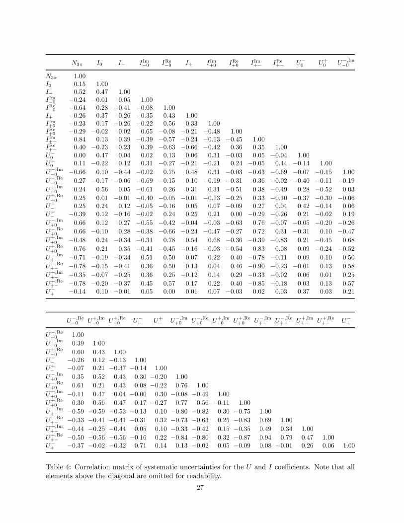
Table 4: Correlation matrix of systematic uncertainties for the U and I coefficients. Note that allelements above the diagonal are omitted for readability.

27

Parameter Description Result

U+0 Coefficient of |f0|2 0.237 ± 0.053 ± 0.043

U+− Coefficient of |f−|2 1.33 ± 0.11 ± 0.04

U−0 Coefficient of |f0|2 cos(ΔmdΔt) −0.055 ± 0.098 ± 0.13

U−− Coefficient of |f−|2 cos(ΔmdΔt) −0.30 ± 0.15 ± 0.03

U−+ Coefficient of |f+|2 cos(ΔmdΔt) 0.53 ± 0.15 ± 0.04

I0 Coefficient of |f0|2 sin(ΔmdΔt) −0.028 ± 0.058 ± 0.02I− Coefficient of |f−|2 sin(ΔmdΔt) −0.03 ± 0.10 ± 0.03I+ Coefficient of |f+|2 sin(ΔmdΔt) 0.039 ± 0.097 ± 0.02

U+,Im+− Coefficient of Im[f+f

∗−] 0.62 ± 0.54 ± 0.72U+,Re

+− Coefficient of Re[f+f∗−] 0.38 ± 0.55 ± 0.28

U−,Im+− Coefficient of Im[f+f

∗−] cos(ΔmdΔt) 0.13 ± 0.94 ± 0.17U−,Re

+− Coefficient of Re[f+f∗−] cos(ΔmdΔt) 2.14 ± 0.91 ± 0.33

IIm+− Coefficient of Im[f+f

∗−] sin(ΔmdΔt) −1.9 ± 1.1 ± 0.1IRe+− Coefficient of Re[f+f

∗−] sin(ΔmdΔt) −0.1 ± 1.9 ± 0.3

U+,Im+0 Coefficient of Im[f+f

∗0 ] 0.03 ± 0.42 ± 0.12

U+,Re+0 Coefficient of Re[f+f

∗0 ] −0.75 ± 0.40 ± 0.15

U−,Im+0 Coefficient of Im[f+f

∗0 ] cos(ΔmdΔt) −0.93 ± 0.68 ± 0.08

U−,Re+0 Coefficient of Re[f+f

∗0 ] cos(ΔmdΔt) −0.47 ± 0.80 ± 0.3

IIm+0 Coefficient of Im[f+f

∗0 ] sin(ΔmdΔt) −0.1 ± 1.1 ± 0.3

IRe+0 Coefficient of Re[f+f

∗0 ] sin(ΔmdΔt) 0.2 ± 1.1 ± 0.4

U+,Im−0 Coefficient of Im[f−f∗0 ] −0.03 ± 0.40 ± 0.23

U+,Re−0 Coefficient of Re[f−f∗0 ] −0.52 ± 0.32 ± 0.08

U−,Im−0 Coefficient of Im[f−f∗0 ] cos(ΔmdΔt) 0.24 ± 0.61 ± 0.2

U−,Re−0 Coefficient of Re[f−f∗0 ] cos(ΔmdΔt) −0.42 ± 0.73 ± 0.28

IIm−0 Coefficient of Im[f−f∗0 ] sin(ΔmdΔt) 0.7 ± 1.0 ± 0.3IRe−0 Coefficient of Re[f−f∗0 ] sin(ΔmdΔt) 0.92 ± 0.91 ± 0.4

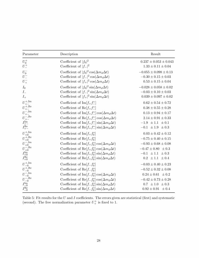
Table 5: Fit results for the U and I coefficients. The errors given are statistical (first) and systematic(second). The free normalization parameter U+

+ is fixed to 1.

28

N3π I0 I− IIm−0 IRe

−0 I+ IIm+0 IRe

+0 IIm+− IRe

+− U−0 U+

0 U−,Im−0

N3π 1.00I0 −0.07 1.00I− −0.06 0.20 1.00IIm−0 0.16 −0.17 −0.12 1.00IRe−0 −0.01 −0.08 −0.13 0.12 1.00I+ 0.03 −0.03 −0.05 0.02 0.27 1.00IIm+0 0.08 0.03 0.11 −0.04 −0.20 −0.36 1.00IRe+0 0.01 0.10 −0.05 0.01 0.29 0.10 −0.07 1.00IIm+− −0.01 0.16 0.28 −0.23 −0.32 −0.11 0.21 −0.06 1.00IRe+− 0.05 −0.00 −0.12 −0.25 −0.01 0.03 −0.04 −0.00 0.07 1.00U−

0 −0.03 0.09 0.23 −0.09 −0.11 −0.04 0.11 −0.08 0.28 0.04 1.00U+

0 0.17 −0.06 −0.01 0.35 0.06 0.01 0.00 0.01 −0.11 −0.27 −0.02 1.00U−,Im−0 −0.05 −0.05 −0.41 −0.09 0.01 0.01 0.03 0.02 0.02 0.11 −0.08 0.02 1.00

U−,Re−0 0.08 −0.16 −0.37 0.20 0.18 0.08 −0.09 0.10 −0.34 0.05 −0.41 0.18 0.25

U+,Im−0 0.05 0.01 −0.07 0.05 −0.00 0.00 0.06 0.03 0.07 −0.00 −0.03 0.15 0.25

U+,Re−0 0.01 −0.01 −0.03 −0.02 −0.01 0.01 0.02 0.01 0.07 −0.01 −0.03 0.09 0.17

U−− −0.02 0.00 0.03 0.07 −0.02 −0.06 0.09 −0.05 0.05 −0.02 0.20 0.05 0.01

U+− 0.12 −0.07 −0.17 0.07 0.10 0.09 0.02 0.09 −0.20 0.04 −0.24 0.04 0.04

U−,Im+0 0.06 0.03 0.07 −0.13 −0.09 −0.15 0.09 0.00 0.20 0.09 0.04 −0.07 0.09

U−,Re+0 0.05 −0.13 −0.29 0.24 0.26 0.31 −0.32 0.09 −0.44 −0.06 −0.37 0.13 0.01

U+,Im+0 0.02 −0.02 −0.11 0.04 0.11 0.23 −0.40 0.10 −0.20 −0.03 −0.21 0.02 −0.03

U+,Re+0 −0.05 −0.01 0.07 −0.02 −0.07 −0.04 −0.03 −0.06 −0.09 −0.04 0.03 −0.02 −0.12

U−,Im+− 0.01 −0.01 0.05 −0.03 −0.03 −0.02 0.07 −0.06 0.11 0.02 0.09 −0.00 0.04

U−,Re+− −0.04 −0.01 0.06 −0.07 0.00 0.01 −0.06 0.06 −0.16 −0.04 −0.02 −0.05 −0.09

U+,Im+− −0.07 0.03 0.06 0.01 −0.04 −0.02 −0.07 0.03 −0.11 −0.07 −0.00 0.01 −0.13

U+,Re+− 0.03 0.01 0.04 −0.05 −0.05 −0.02 0.08 0.01 0.17 0.04 0.06 −0.03 0.06

U−+ 0.02 0.04 0.00 −0.06 −0.02 0.01 −0.01 0.07 0.04 0.04 0.17 −0.02 0.01

U−,Re−0 U+,Im

−0 U+,Re−0 U−

− U+− U−,Im

+0 U−,Re+0 U+,Im

+0 U+,Re+0 U−,Im

+− U−,Re+− U+,Im

+− U+,Re+− U−

+

U−,Re−0 1.00

U+,Im−0 0.12 1.00

U+,Re−0 0.04 0.07 1.00

U−− 0.09 0.04 −0.13 1.00

U+− 0.24 0.00 0.01 −0.07 1.00

U−,Im+0 −0.04 0.08 0.05 −0.00 0.26 1.00

U−,Re+0 0.40 −0.04 −0.02 −0.08 0.32 −0.14 1.00

U+,Im+0 0.09 −0.02 0.02 −0.26 0.17 −0.09 0.35 1.00

U+,Re+0 −0.19 −0.10 −0.11 −0.03 −0.05 −0.07 −0.04 0.03 1.00

U−,Im+− −0.05 0.03 0.12 0.09 −0.05 0.08 −0.09 −0.12 −0.01 1.00

U−,Re+− −0.17 −0.13 −0.03 −0.10 −0.02 −0.05 −0.04 0.08 0.35 −0.02 1.00

U+,Im+− −0.19 −0.10 −0.03 −0.04 −0.07 −0.15 0.01 0.07 0.25 −0.01 0.18 1.00

U+,Re+− 0.02 0.05 −0.03 0.14 0.11 0.30 −0.09 −0.13 −0.03 0.16 −0.10 −0.11 1.00

U−+ −0.00 0.01 0.06 −0.05 0.08 0.06 −0.04 0.07 −0.05 −0.06 −0.04 −0.10 −0.04 1.00

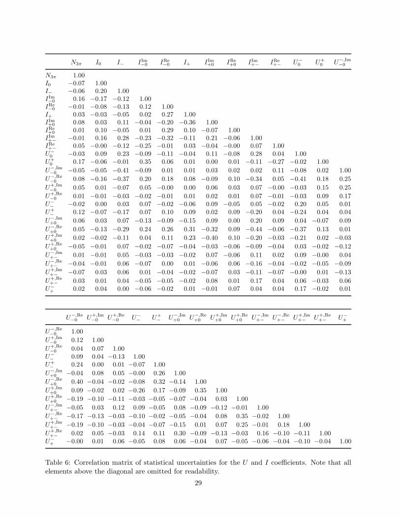
Table 6: Correlation matrix of statistical uncertainties for the U and I coefficients. Note that allelements above the diagonal are omitted for readability.

29

ΔE'

Eve

nts

/ 0.1

3

0

50

100

150

200

-1 -0.5 0 0.5 10

50

100

150

5.275 5.28 5.285

mES (GeV/c2)

Eve

nts

/ 0.0

011G

eV/c

2 BABARP R E L I M I N A R Y

NN output

Eve

nts

/ 0.0

84

0

25

50

75

100

0 0.5 1

Δt/σ(Δt)

Eve

nts

/ 1.5

10

10 2

-10 0 10

m'

Eve

nts

/ 0.0

7

0

50

100

0 0.2 0.4 0.6 0.8 1

θ'

Eve

nts

/ 0.0

7

0

50

100

0 0.2 0.4 0.6 0.8 1

Figure 3: Distributions of (top to bottom, left to right) ΔE ′, mES, NN output, Δt/σ(Δt), m′ andθ′ for samples enhanced in B0 → π+π−π0 signal. The dots with error bars give the on-resonancedata. The solid histogram shows the projection of the fit result. The dark, medium and lightshaded areas represent respectively the contribution from continuum events, the sum of continuumevents and the B-background expectation, and the sum of these and the misreconstructed signalevents.

30

0

50

100

0.5 1 1.5 2

mmin (GeV/c2)

Eve

nts

/ 0.0

4GeV

/c2

BABARP R E L I M I N A R Y

Figure 4: Distribution of minimum of the three di-pion invariant masses, for samples enhanced inB0 → π+π−π0 signal. The dots with error bars give the on-resonance data. The solid histogramshows the projection of the fit result. The dark, medium and light shaded areas represent respec-tively the contribution from continuum events, the sum of continuum events and the B-backgroundexpectation, and the sum of these and the misreconstructed signal events.

Aρπ C ΔC S ΔS

Aρπ 1.93C −0.71 9.68ΔC −0.55 2.63 8.93S −0.03 −0.71 −0.13 15.3ΔS −0.03 −0.57 −0.07 3.93 17.08

Table 7: Covariance matirx multipled by 1000 of the quasi-two-body parameters.

31

-1

-0.75

-0.5

-0.25

0

0.25

0.5

0.75

1

-1 -0.75 -0.5 -0.25 0 0.25 0.5 0.75 1

A– +

ρπ

A+

– ρπ

BABARP R E L I M I N A R Y

Figure 5: Confidence level contours for the direct CP asymmetries A+−ρπ versus A−+

ρπ . The shadedareas represent 1σ, 2σ and 3σ contours, respectively.

0

0.25

0.5

0.75

1

-100 0 100

δ+- (deg)

C.L

.

B A B A RP R E L I M I N A R Y

0

0.25

0.5

0.75

1

0 50 100 150

α (deg)

C.L

.

B A B A RP R E L I M I N A R Y

Figure 6: Confidence level functions for δ+− (left) and α (right). Indicated by the dashed horizontallines are the confidence level (C.L.) values corresponding to 1σ and 2σ, respectively.

32