Kailai Xu Stanford University

Machine Learning for Computational Engineering

Kailai XuStanford University

Kailai Xu 1 / 50

Outline

1 Inverse Modeling

2 Software Implementation

3 First Order Physics Constrained Learning

4 Second Order Physics Constrained Learning

5 Conclusion

Kailai Xu Inverse Modeling 2 / 50

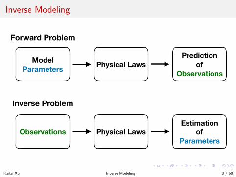
Inverse Modeling

Forward Problem

Inverse Problem

Model Parameters

Observations

Physical Laws

Physical LawsEstimation

of Parameters

Prediction of

Observations


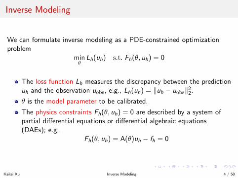
Inverse Modeling

We can formulate inverse modeling as a PDE-constrained optimizationproblem

minθ

Lh(uh) s.t. Fh(θ, uh) = 0

The loss function Lh measures the discrepancy between the predictionuh and the observation uobs, e.g., Lh(uh) = ‖uh − uobs‖2

2.

θ is the model parameter to be calibrated.

The physics constraints Fh(θ, uh) = 0 are described by a system ofpartial differential equations or differential algebraic equations(DAEs); e.g.,

Fh(θ, uh) = A(θ)uh − fh = 0


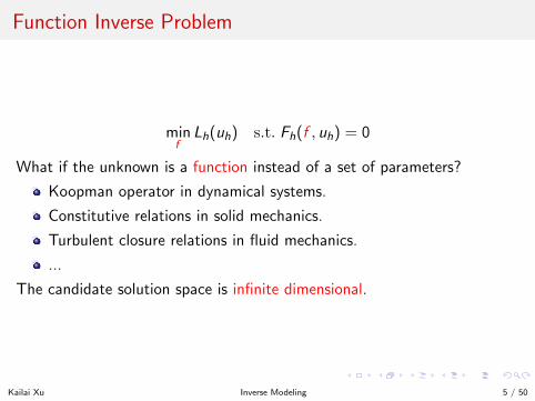
Function Inverse Problem

minf

Lh(uh) s.t. Fh(f , uh) = 0

What if the unknown is a function instead of a set of parameters?

Koopman operator in dynamical systems.

Constitutive relations in solid mechanics.

Turbulent closure relations in fluid mechanics.

...

The candidate solution space is infinite dimensional.


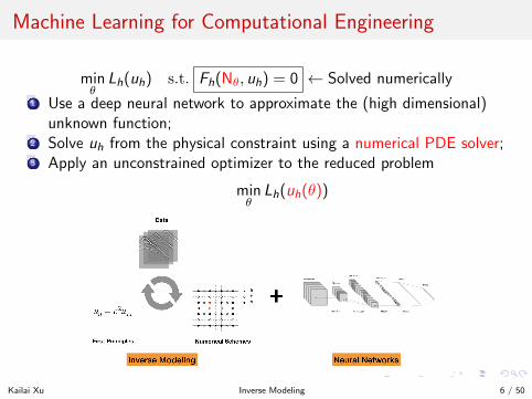
Machine Learning for Computational Engineering

minθ

Lh(uh) s.t. Fh(Nθ, uh) = 0 ← Solved numerically

1 Use a deep neural network to approximate the (high dimensional)unknown function;

2 Solve uh from the physical constraint using a numerical PDE solver;3 Apply an unconstrained optimizer to the reduced problem

minθ

Lh(uh(θ))


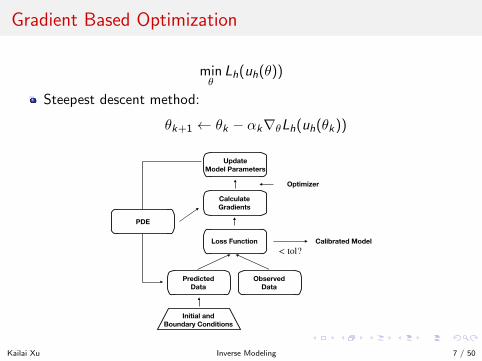
Gradient Based Optimization

minθ

Lh(uh(θ))

Steepest descent method:

θk+1 ← θk − αk∇θLh(uh(θk))

Predicted Data

Observed Data

Loss Function

Calculate Gradients

Update Model Parameters

PDE

Initial and Boundary Conditions

Optimizer

< tol?Calibrated Model


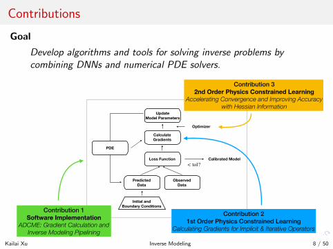
Contributions

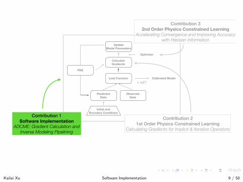
Goal

Develop algorithms and tools for solving inverse problems bycombining DNNs and numerical PDE solvers.

Predicted Data

Observed Data

Loss Function

Calculate Gradients


PDE


Optimizer


Contribution 2 1st Order Physics Constrained Learning

Calculating Gradients for Implicit & Iterative Operators

Contribution 3 2nd Order Physics Constrained Learning

Accelerating Convergence and Improving Accuracy with Hessian Information

Contribution 1 Software Implementation

ADCME: Gradient Calculation and Inverse Modeling Pipelining


Predicted Data

Observed Data

Loss Function

Calculate Gradients


PDE


Optimizer








Kailai Xu Software Implementation 9 / 50

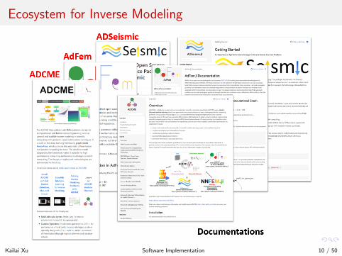
Ecosystem for Inverse Modeling


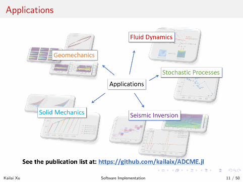
Applications


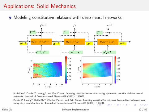
Applications: Solid Mechanics

Modeling constitutive relations with deep neural networks

Mθ(ǫi, ǫi−1,σi−1)

Li

σi−1

fi

σi Mθ(ǫ

i+1, ǫi,σi)

Li+1

fi+1

σi+1

Mθ(ǫi−1, ǫi−2,σi−2)

Li−1

σi−2

fi−1

ǫi−2, ǫi−1

0 2 4 6 8 10X (cm)

0

2

4

6

Y (c

m)

0.25

0.50

0.75

1.00

1.25

1.50

1.75

Kailai Xu*, Daniel Z. Huang*, and Eric Darve. Learning constitutive relations using symmetric positive definite neuralnetworks. Journal of Computational Physics 428 (2021): 110072.

Daniel Z. Huang*, Kailai Xu*, Charbel Farhat, and Eric Darve. Learning constitutive relations from indirect observationsusing deep neural networks. Journal of Computational Physics 416 (2020): 109491.


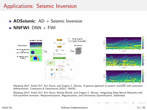
Applications: Seismic Inversion

ADSeismic: AD + Seismic Inversion

NNFWI: DNN + FWI

0 2 4 6 8 10X (km)

0

1

2

3

Z (k

m)

2

3

4

km/s

0 2 4 6 8 10X (km)

0

1

2

3

Z (k

m)

2

3

4

km/s

0 2 4 6 8 10X (km)

0

1

2

3

Z (k

m)

2

3

4

km/s

Weiqiang Zhu*, Kailai Xu*, Eric Darve, and Gregory C. Beroza. A general approach to seismic inversion with automaticdifferentiation. Computers & Geosciences (2021): 104751.

Weiqiang Zhu*, Kailai Xu*, Eric Darve, Biondo Biondi, and Gregory C. Beroza. Integrating Deep Neural Networks withFull-waveform Inversion: Reparametrization, Regularization, and Uncertainty Quantification. Submitted.


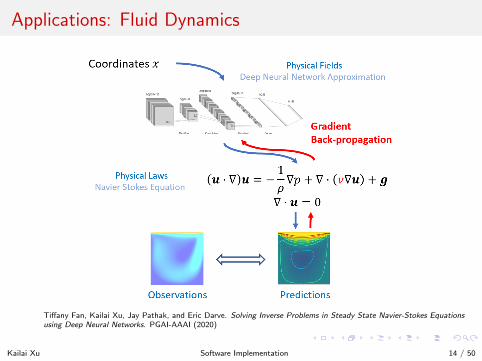
Applications: Fluid Dynamics

Tiffany Fan, Kailai Xu, Jay Pathak, and Eric Darve. Solving Inverse Problems in Steady State Navier-Stokes Equationsusing Deep Neural Networks. PGAI-AAAI (2020)


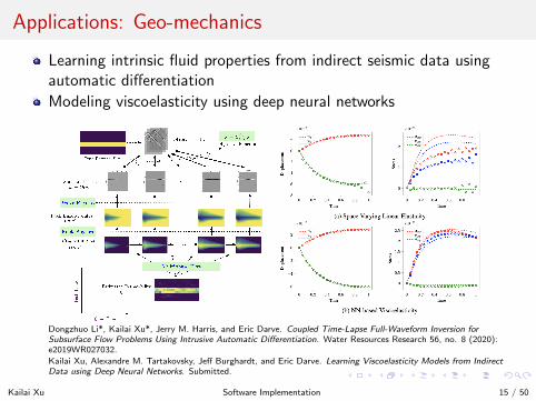
Applications: Geo-mechanics

Learning intrinsic fluid properties from indirect seismic data usingautomatic differentiation

Modeling viscoelasticity using deep neural networks

Dongzhuo Li*, Kailai Xu*, Jerry M. Harris, and Eric Darve. Coupled Time-Lapse Full-Waveform Inversion forSubsurface Flow Problems Using Intrusive Automatic Differentiation. Water Resources Research 56, no. 8 (2020):e2019WR027032.

Kailai Xu, Alexandre M. Tartakovsky, Jeff Burghardt, and Eric Darve. Learning Viscoelasticity Models from IndirectData using Deep Neural Networks. Submitted.


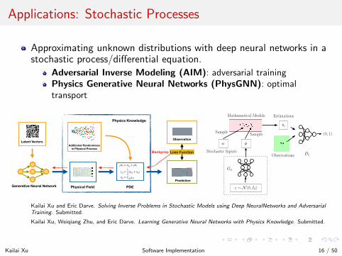
Applications: Stochastic Processes

Approximating unknown distributions with deep neural networks in astochastic process/differential equation.

Adversarial Inverse Modeling (AIM): adversarial trainingPhysics Generative Neural Networks (PhysGNN): optimaltransport

Generative Neural Network

ρ··ui = σij,j + ρbi

εij = 12 (uj,i + ui,j)

σij = Cijklεkl

Physical Field PDE

Prediction

Additional Randomness in Physical Process

Latent VectorsObservation

Loss FunctionBackprop

Physics Knowledge

θw

ui

(0, 1)

ObservationsStochastic Inputs

Mathematical Models Estimations

Dξ

z ∼ N (0, Id)

Gη

SampleSample

Kailai Xu and Eric Darve. Solving Inverse Problems in Stochastic Models using Deep NeuralNetworks and AdversarialTraining. Submitted.

Kailai Xu, Weiqiang Zhu, and Eric Darve. Learning Generative Neural Networks with Physics Knowledge. Submitted.


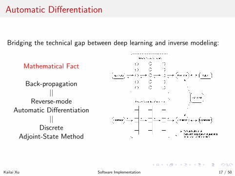
Automatic Differentiation

Bridging the technical gap between deep learning and inverse modeling:

Mathematical Fact

Back-propagation||

Reverse-modeAutomatic Differentiation

||Discrete

Adjoint-State Method


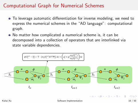
Computational Graph for Numerical Schemes

To leverage automatic differentiation for inverse modeling, we need toexpress the numerical schemes in the “AD language”: computationalgraph.

No matter how complicated a numerical scheme is, it can bedecomposed into a collection of operators that are interlinked viastate variable dependencies.

S2

u ϕ

mtΨ2

ϕ(Sn+12 − Sn2) − ∇ ⋅ (m2(Sn+1

2 )K ∇Ψn2) Δt = (qn2 + qn1m2(Sn+12 )m1(Sn+12 ) ) Δt

S2

u ϕ

mtΨ2

S2

u ϕ

mtΨ2

tn tn+1 tn+2


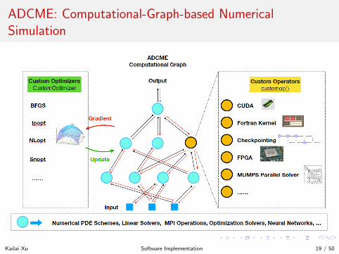
ADCME: Computational-Graph-based NumericalSimulation


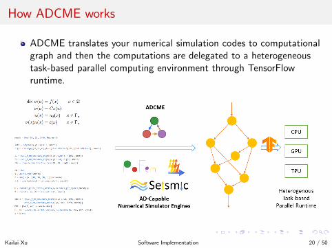
How ADCME works

ADCME translates your numerical simulation codes to computationalgraph and then the computations are delegated to a heterogeneoustask-based parallel computing environment through TensorFlowruntime.


Summary

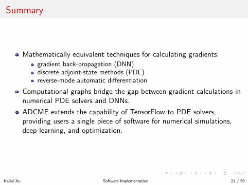
Mathematically equivalent techniques for calculating gradients:

gradient back-propagation (DNN)discrete adjoint-state methods (PDE)reverse-mode automatic differentiation

Computational graphs bridge the gap between gradient calculations innumerical PDE solvers and DNNs.

ADCME extends the capability of TensorFlow to PDE solvers,providing users a single piece of software for numerical simulations,deep learning, and optimization.


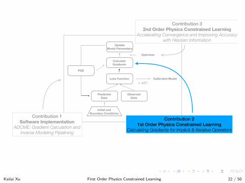
Predicted Data

Observed Data

Loss Function

Calculate Gradients


PDE


Optimizer








Kailai Xu First Order Physics Constrained Learning 22 / 50

Motivation

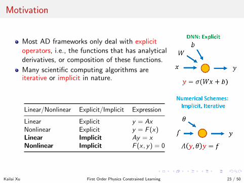
Most AD frameworks only deal with explicitoperators, i.e., the functions that has analyticalderivatives, or composition of these functions.

Many scientific computing algorithms areiterative or implicit in nature.

Linear/Nonlinear Explicit/Implicit Expression

Linear Explicit y = AxNonlinear Explicit y = F (x)Linear Implicit Ay = xNonlinear Implicit F (x , y) = 0


Example

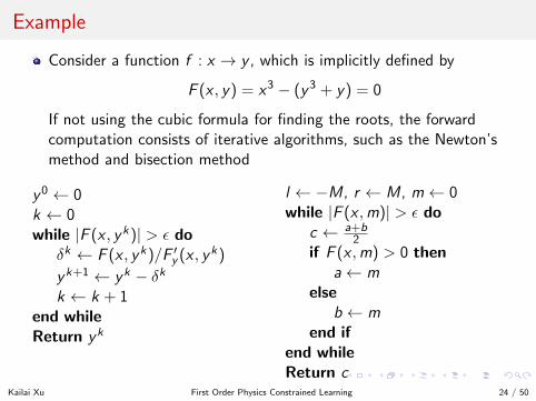
Consider a function f : x → y , which is implicitly defined by

F (x , y) = x3 − (y3 + y) = 0

If not using the cubic formula for finding the roots, the forwardcomputation consists of iterative algorithms, such as the Newton’smethod and bisection method

y0 ← 0k ← 0while |F (x , yk)| > ε do

δk ← F (x , yk)/F ′y (x , yk)

yk+1 ← yk − δkk ← k + 1

end whileReturn yk

l ← −M, r ← M, m← 0while |F (x ,m)| > ε do

c ← a+b2

if F (x ,m) > 0 thena← m

elseb ← m

end ifend whileReturn c


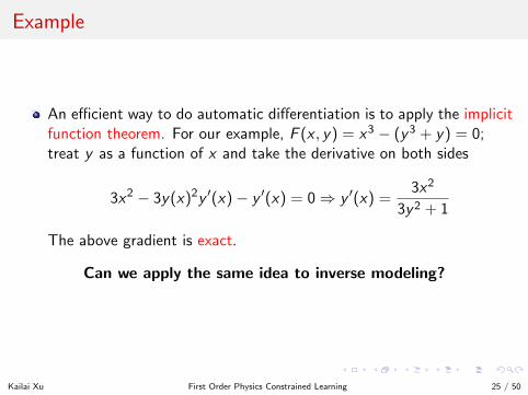
Example

An efficient way to do automatic differentiation is to apply the implicitfunction theorem. For our example, F (x , y) = x3 − (y3 + y) = 0;treat y as a function of x and take the derivative on both sides

3x2 − 3y(x)2y ′(x)− y ′(x) = 0⇒ y ′(x) =3x2

3y2 + 1

The above gradient is exact.

Can we apply the same idea to inverse modeling?


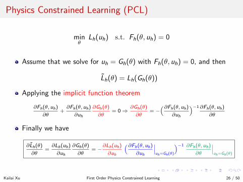
Physics Constrained Learning (PCL)

minθ

Lh(uh) s.t. Fh(θ, uh) = 0

Assume that we solve for uh = Gh(θ) with Fh(θ, uh) = 0, and then

Lh(θ) = Lh(Gh(θ))

Applying the implicit function theorem

∂Fh(θ, uh)

∂θ+∂Fh(θ, uh)

∂uh

∂Gh(θ)

∂θ= 0⇒

∂Gh(θ)

∂θ= −

(∂Fh(θ, uh)

∂uh

)−1 ∂Fh(θ, uh)

∂θ

Finally we have

∂Lh(θ)

∂θ=∂Lh(uh)

∂uh

∂Gh(θ)

∂θ= −

∂Lh(uh)

∂uh

(∂Fh(θ, uh)

∂uh

∣∣∣uh=Gh(θ)

)−1 ∂Fh(θ, uh)

∂θ

∣∣∣uh=Gh(θ)


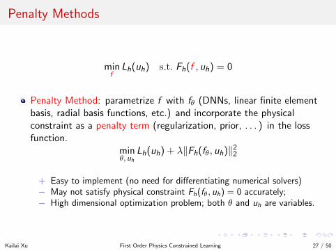
Penalty Methods

minf


Penalty Method: parametrize f with fθ (DNNs, linear finite elementbasis, radial basis functions, etc.) and incorporate the physicalconstraint as a penalty term (regularization, prior, . . . ) in the lossfunction.

minθ, uh

Lh(uh) + λ‖Fh(fθ, uh)‖22

+ Easy to implement (no need for differentiating numerical solvers)− May not satisfy physical constraint Fh(fθ, uh) = 0 accurately;− High dimensional optimization problem; both θ and uh are variables.


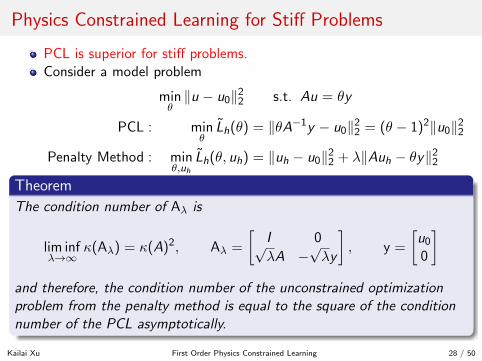
Physics Constrained Learning for Stiff Problems

PCL is superior for stiff problems.Consider a model problem

minθ‖u − u0‖2

2 s.t. Au = θy

PCL : minθ

Lh(θ) = ‖θA−1y − u0‖22 = (θ − 1)2‖u0‖2

2

Penalty Method : minθ,uh

Lh(θ, uh) = ‖uh − u0‖22 + λ‖Auh − θy‖2

2

Theorem

The condition number of Aλ is

lim infλ→∞

κ(Aλ) = κ(A)2, Aλ =

[I 0√λA −

√λy

], y =

[u0

0

]and therefore, the condition number of the unconstrained optimizationproblem from the penalty method is equal to the square of the conditionnumber of the PCL asymptotically.


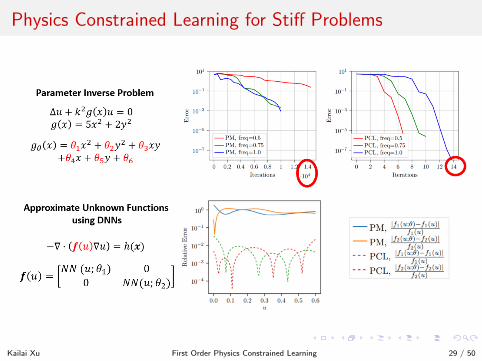
Physics Constrained Learning for Stiff Problems


Summary

Implicit and iterative operators are ubiquitous in numerical PDEsolvers. These operators are insufficiently treated in deep learningsoftware and frameworks.

PCL helps you calculate gradients of implicit/iterative operatorsefficiently.

PCL leads to faster convergence and better accuracy compared topenalty methods for stiff problems.


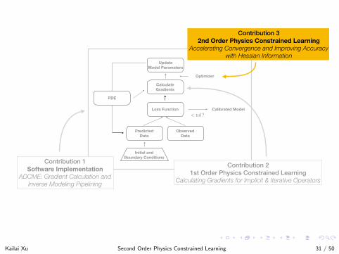
Predicted Data

Observed Data

Loss Function

Calculate Gradients


PDE


Optimizer








Kailai Xu Second Order Physics Constrained Learning 31 / 50

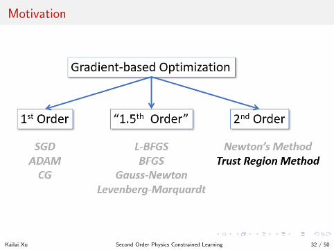
Motivation


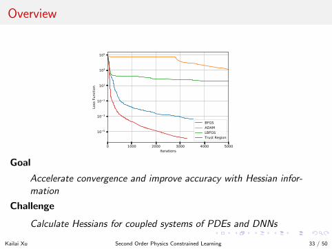
Overview

0 1000 2000 3000 4000 5000Iterations

10 5

10 3

10 1

101

103

105

Loss

Fun

ctio

n

BFGSADAMLBFGSTrust Region

Goal

Accelerate convergence and improve accuracy with Hessian infor-mation

Challenge

Calculate Hessians for coupled systems of PDEs and DNNs


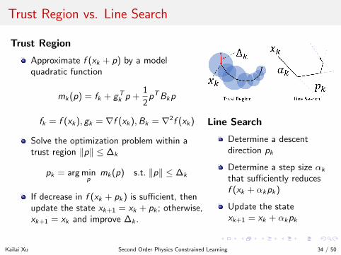
Trust Region vs. Line Search

Trust Region

Approximate f (xk + p) by a modelquadratic function

mk(p) = fk + gTk p +

1

2pTBkp

fk = f (xk), gk = ∇f (xk),Bk = ∇2f (xk)

Solve the optimization problem within atrust region ‖p‖ ≤ ∆k

pk = arg minp

mk(p) s.t. ‖p‖ ≤ ∆k

If decrease in f (xk + pk) is sufficient, thenupdate the state xk+1 = xk + pk ; otherwise,xk+1 = xk and improve ∆k .

Line Search

Determine a descentdirection pk

Determine a step size αk

that sufficiently reducesf (xk + αkpk)

Update the statexk+1 = xk + αkpk


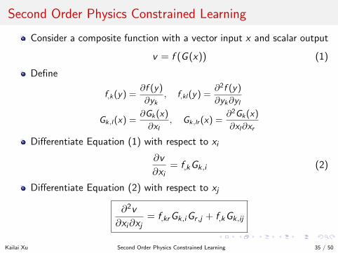
Second Order Physics Constrained Learning

Consider a composite function with a vector input x and scalar output

v = f (G (x)) (1)

Define

f,k(y) =∂f (y)

∂yk, f,kl(y) =

∂2f (y)

∂yk∂yl

Gk,l(x) =∂Gk(x)

∂xl, Gk,lr (x) =

∂2Gk(x)

∂xl∂xr

Differentiate Equation (1) with respect to xi

∂v

∂xi= f,kGk,i (2)

Differentiate Equation (2) with respect to xj

∂2v

∂xi∂xj= f,krGk,iGr ,j + f,kGk,ij


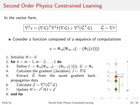
Second Order Physics Constrained Learning

In the vector form,

∇2v = (∇G )T∇2f (∇G ) +∇2(GTG ) G = ∇f

Consider a function composed of a sequence of computations

v = Φm(Φm−1(· · · (Φ1(z))))

1: Initialize H ← 02: for k = m − 1,m − 2, . . . , 1 do3: Define f := Φm(Φm−1(· · · (Φk+1(·)))), G := Φk

4: Calculate the gradient (Jacobian) J ← ∇G5: Extract G from the saved gradient back-

propagation data6: Calculate Z = ∇2(GTG )7: Update H ← JTHJ + Z8: end for


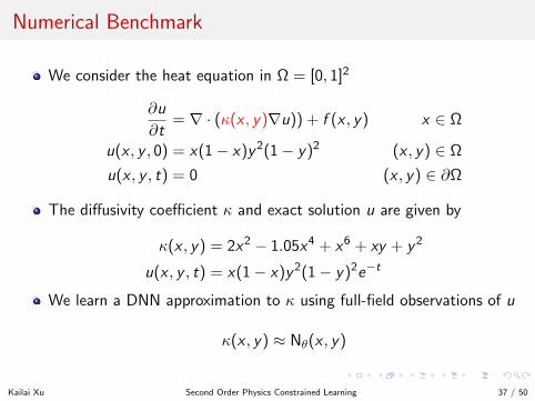
Numerical Benchmark

We consider the heat equation in Ω = [0, 1]2

∂u

∂t= ∇ · (κ(x , y)∇u)) + f (x , y) x ∈ Ω

u(x , y , 0) = x(1− x)y2(1− y)2 (x , y) ∈ Ω

u(x , y , t) = 0 (x , y) ∈ ∂Ω

The diffusivity coefficient κ and exact solution u are given by

κ(x , y) = 2x2 − 1.05x4 + x6 + xy + y2

u(x , y , t) = x(1− x)y2(1− y)2e−t

We learn a DNN approximation to κ using full-field observations of u

κ(x , y) ≈ Nθ(x , y)


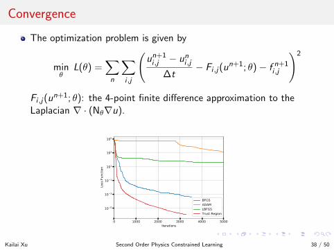
Convergence

The optimization problem is given by

minθ

L(θ) =∑n

∑i ,j

(un+1i ,j − uni ,j

∆t− Fi ,j(u

n+1; θ)− f n+1i ,j

)2

Fi ,j(un+1; θ): the 4-point finite difference approximation to the

Laplacian ∇ · (Nθ∇u).

0 1000 2000 3000 4000 5000Iterations

10 5

10 3

10 1

101

103

105

Loss

Fun

ctio

n

BFGSADAMLBFGSTrust Region


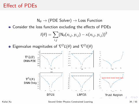
Effect of PDEs

Nθ → (PDE Solver)→ Loss Function

Consider the loss function excluding the effects of PDEs

l(θ) =∑i ,j

(Nθ(xi ,j , yi ,j)− κ(xi ,j , yi ,j))2

Eigenvalue magnitudes of ∇2L(θ) and ∇2l(θ)


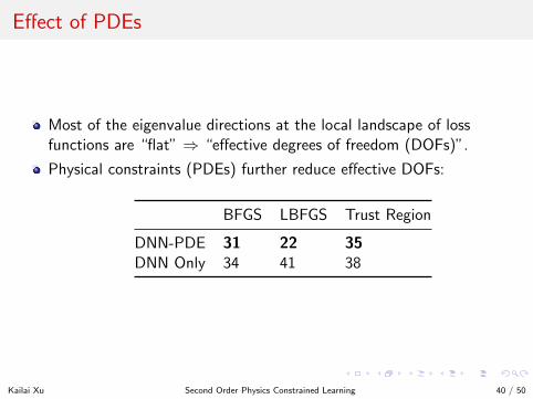
Effect of PDEs

Most of the eigenvalue directions at the local landscape of lossfunctions are “flat” ⇒ “effective degrees of freedom (DOFs)”.

Physical constraints (PDEs) further reduce effective DOFs:

BFGS LBFGS Trust Region

DNN-PDE 31 22 35DNN Only 34 41 38


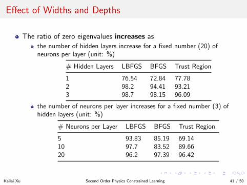
Effect of Widths and Depths

The ratio of zero eigenvalues increases as

the number of hidden layers increase for a fixed number (20) ofneurons per layer (unit: %)

# Hidden Layers LBFGS BFGS Trust Region

1 76.54 72.84 77.782 98.2 94.41 93.213 98.7 98.15 96.09

the number of neurons per layer increases for a fixed number (3) ofhidden layers (unit: %)

# Neurons per Layer LBFGS BFGS Trust Region

5 93.83 85.19 69.1410 97.7 83.52 89.6620 96.2 97.39 96.42


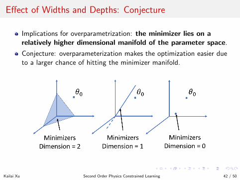
Effect of Widths and Depths: Conjecture

Implications for overparametrization: the minimizer lies on arelatively higher dimensional manifold of the parameter space.

Conjecture: overparameterization makes the optimization easier dueto a larger chance of hitting the minimizer manifold.


Summary

Trust region methods converge significantly faster compared to firstorder/quasi second order methods by leveraging Hessian information.

Second order physics constrained learning helps you calculate Hessianmatrices efficiently.

The local minimum of DNNs have small effective degrees of freedomcompared to DNN sizes.


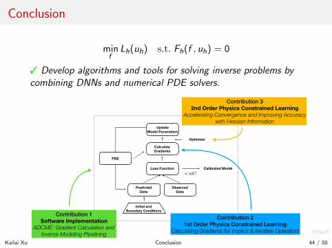
Conclusion

minf


3 Develop algorithms and tools for solving inverse problems bycombining DNNs and numerical PDE solvers.

Predicted Data

Observed Data

Loss Function

Calculate Gradients


PDE


Optimizer








Kailai Xu Conclusion 44 / 50

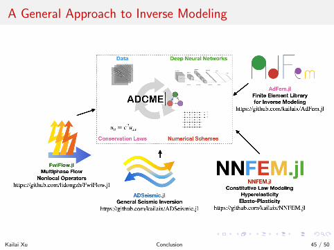
A General Approach to Inverse Modeling


Supporting Materials


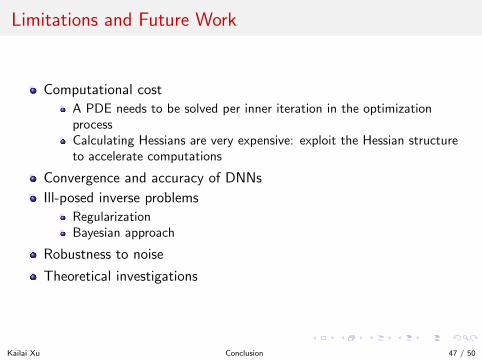
Limitations and Future Work

Computational cost

A PDE needs to be solved per inner iteration in the optimizationprocessCalculating Hessians are very expensive: exploit the Hessian structureto accelerate computations

Convergence and accuracy of DNNs

Ill-posed inverse problems

RegularizationBayesian approach

Robustness to noise

Theoretical investigations


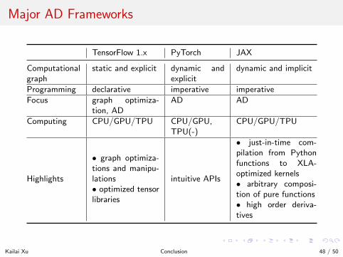
Major AD Frameworks

TensorFlow 1.x PyTorch JAX

Computationalgraph

static and explicit dynamic andexplicit

dynamic and implicit

Programming declarative imperative imperative

Focus graph optimiza-tion, AD

AD AD

Computing CPU/GPU/TPU CPU/GPU,TPU(-)

CPU/GPU/TPU

Highlights

• graph optimiza-tions and manipu-lations• optimized tensorlibraries

intuitive APIs

• just-in-time com-pilation from Pythonfunctions to XLA-optimized kernels• arbitrary composi-tion of pure functions• high order deriva-tives


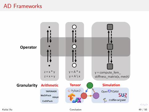
AD Frameworks

z = x * yz = x + y

y = A * xy = A \ x

y = compute_fem_stiffness_matrix(x, mesh)

Operator

Arithmetic Tensor SimulationGranularity

MeDiPack

CoDiPack

Adept

TAPENADE


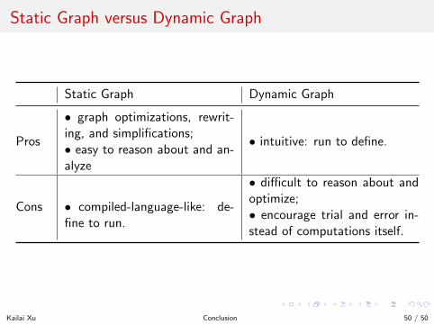
Static Graph versus Dynamic Graph

Static Graph Dynamic Graph

Pros

• graph optimizations, rewrit-ing, and simplifications;• easy to reason about and an-alyze

• intuitive: run to define.

Cons • compiled-language-like: de-fine to run.

• difficult to reason about andoptimize;• encourage trial and error in-stead of computations itself.


Kailai Xu Stanford University

Documents

Transcript of Kailai Xu Stanford University