A1, General Physics Experiment I M a L b T c Spring ...

A1, General Physics Experiment I [M ]a[L]b[T ]c Spring Semester, 2021

Name:

Team No. :

Department:

Date :

Student ID:

Lecturer’s Signature :

Introduction

1. E1: Free Fall

Goals

• Practice the video tracking analysis.

• Understand the χ2 method as an example ofthe goodness of fit tests.

• Estimate the gravitational acceleration g.

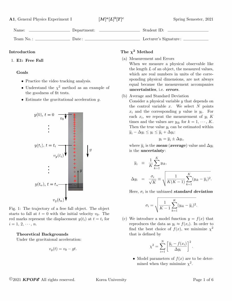
Fig. 1: The trajectory of a free fall object. The objectstarts to fall at t = 0 with the initial velocity v0. Thered marks represent the displacement y(ti) at t = ti fori = 1, 2, · · · , n.

Theoretical BackgroundsUnder the gravitaional acceleration:

vy(t) = v0 − gt.

The χ2 Method

(a) Measurement and ErrorsWhen we measure a physical observable likethe length L of an object, the measured values,which are real numbers in units of the corre-sponding physical dimensions, are not alwaysequal because the measurement accompaniesuncertainties, i.e. errors.

(b) Average and Standard DeviationConsider a physical variable y that depends onthe control variable x. We select N pointsxi and the corresponding y value is yi. Foreach xi, we repeat the measurement of yi Ktimes and the values are yik for k = 1, · · · , K.Then the true value yi can be estimated withinyi −∆yi ≤ yi ≤ yi + ∆yi:

yi = yi ±∆yi,

where yi is the mean (average) value and ∆yiis the uncertainty :

yi ≡1

K

K∑k=1

yik,

∆yi =σi√K≡

√√√√ 1

K(K − 1)

K∑k=1

(yik − yi)2.

Here, σi is the unbiased standard deviation

σi =

√√√√ 1

K − 1

K∑k=1

(yik − yi)2.

(c) We introduce a model function y = f(x) thatreproduces the data as yi ≈ f(xi). In order tofind the best choice of f(x), we minimize χ2

that is defined by

χ2 =N∑i=1

[yi − f(xi)

∆yi

]2.

• Model parameters of f(x) are to be deter-mined when they minimize χ2.

©2021 KPOPEEE All rights reserved. Korea University of 6


• When the model fits the data well, χ2 →the number of degrees of freedom N −M .Here, N is the number of random variablesand M is the number of model parametersin y = f(x).

2. E2: Projectile Motion

Goal

• Understand the projectile motion.

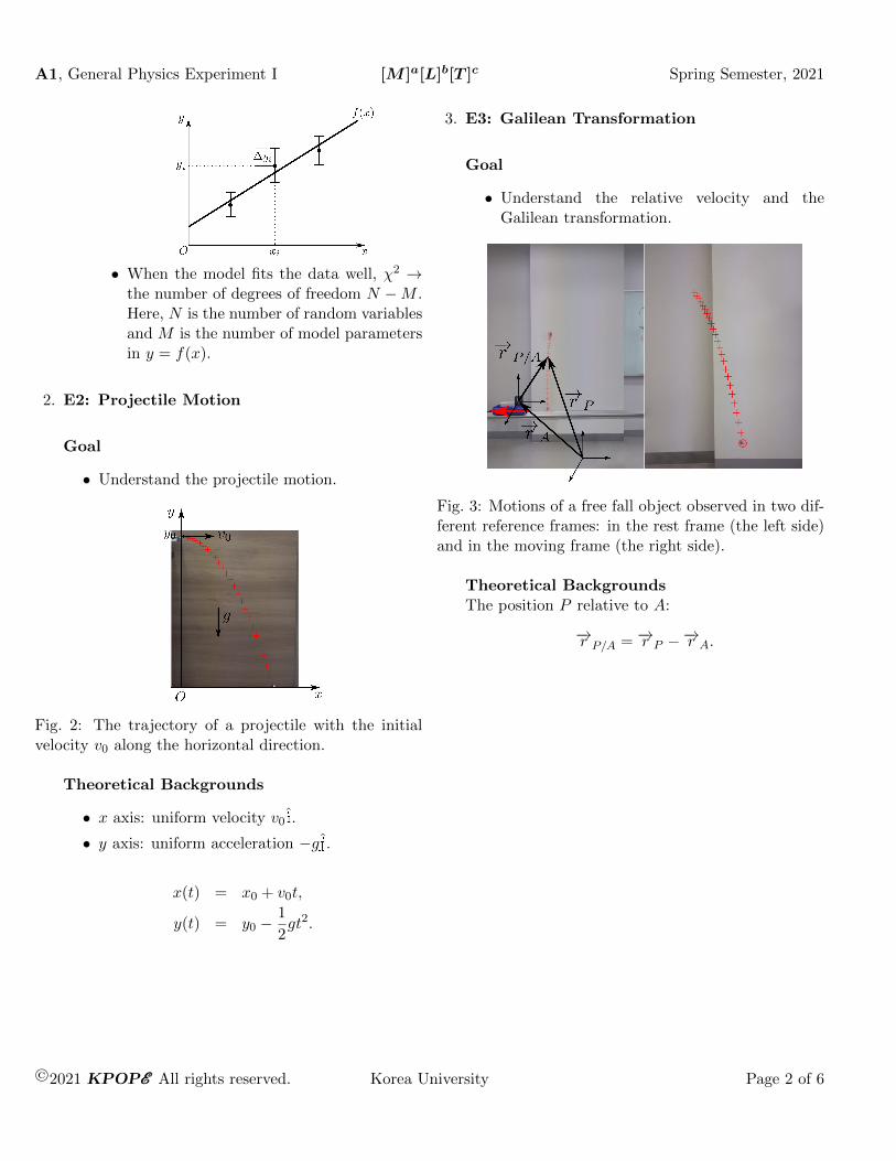
Fig. 2: The trajectory of a projectile with the initialvelocity v0 along the horizontal direction.

Theoretical Backgrounds

• x axis: uniform velocity v0i.

• y axis: uniform acceleration −gj.

x(t) = x0 + v0t,

y(t) = y0 −1

2gt2.

3. E3: Galilean Transformation

Goal

• Understand the relative velocity and theGalilean transformation.

Fig. 3: Motions of a free fall object observed in two dif-ferent reference frames: in the rest frame (the left side)and in the moving frame (the right side).

Theoretical BackgroundsThe position P relative to A:

−→r P/A = −→r P −−→r A.



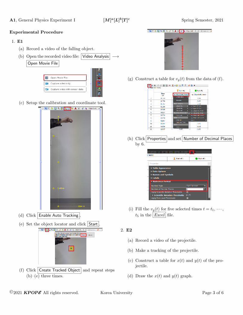
Experimental Procedure

1. E1

(a) Record a video of the falling object.

(b) Open the recorded video file: Video Analysis −→Open Movie File

(c) Setup the calibration and coordinate tool.

(d) Click Enable Auto Tracking .

(e) Set the object locator and click Start .

(f) Click Create Tracked Object and repeat steps

(b)–(e) three times.

(g) Construct a table for vy(t) from the data of (f).

(h) Click Properties and set Number of Decimal Placesby 6.

(i) Fill the vy(t) for five selected times t = t1, · · · ,t5 in the Excel file.

2. E2

(a) Record a video of the projectile.

(b) Make a tracking of the projectile.

(c) Construct a table for x(t) and y(t) of the pro-jectile.

(d) Draw the x(t) and y(t) graph.



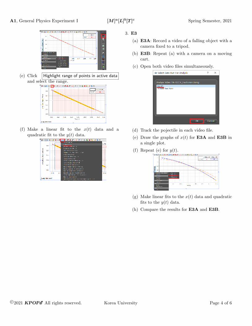
(e) Click Highlight range of points in active dataand select the range.

(f) Make a linear fit to the x(t) data and aquadratic fit to the y(t) data.

3. E3

(a) E3A: Record a video of a falling object with acamera fixed to a tripod.

(b) E3B: Repeat (a) with a camera on a movingcart.

(c) Open both video files simultaneously.

(d) Track the pojectile in each video file.

(e) Draw the graphs of x(t) for E3A and E3B ina single plot.

(f) Repeat (e) for y(t).

(g) Make linear fits to the x(t) data and quadraticfits to the y(t) data.

(h) Compare the results for E3A and E3B.



Name:

Team No. :

Department:

Date :

Student ID:

Lecturer’s Signature :

Discussion (7 points)

Problem 1Problem 2



Problem 3


A1, General Physics Experiment I M a L b T c Spring ...

Documents

Transcript of A1, General Physics Experiment I M a L b T c Spring ...