A Visual Αnalysis of Calculation-Paths of the …...application and use of fractals has been...

$: A Visual Αnalysis of Calculation-Paths of the …...application and use of fractals has been increasing with the increase of computer power. They have shown their usability in a wide$
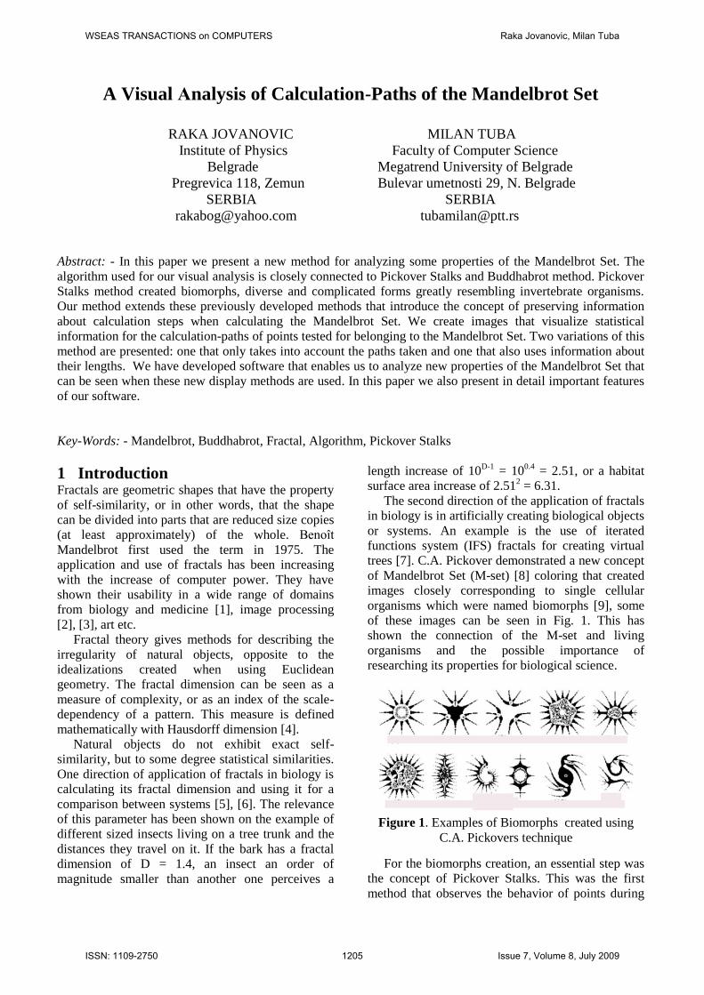
A Visual Αnalysis of Calculation-Paths of the Mandelbrot Set

RAKA JOVANOVIC MILAN TUBA

Institute of Physics Faculty of Computer Science

Belgrade Megatrend University of Belgrade

Pregrevica 118, Zemun Bulevar umetnosti 29, N. Belgrade

SERBIA SERBIA

[email protected] [email protected]

Abstract: - In this paper we present a new method for analyzing some properties of the Mandelbrot Set. The

algorithm used for our visual analysis is closely connected to Pickover Stalks and Buddhabrot method. Pickover

Stalks method created biomorphs, diverse and complicated forms greatly resembling invertebrate organisms.

Our method extends these previously developed methods that introduce the concept of preserving information

about calculation steps when calculating the Mandelbrot Set. We create images that visualize statistical

information for the calculation-paths of points tested for belonging to the Mandelbrot Set. Two variations of this

method are presented: one that only takes into account the paths taken and one that also uses information about

their lengths. We have developed software that enables us to analyze new properties of the Mandelbrot Set that

can be seen when these new display methods are used. In this paper we also present in detail important features

of our software.

Key-Words: - Mandelbrot, Buddhabrot, Fractal, Algorithm, Pickover Stalks

1 Introduction Fractals are geometric shapes that have the property

of self-similarity, or in other words, that the shape

can be divided into parts that are reduced size copies

(at least approximately) of the whole. Benoît

Mandelbrot first used the term in 1975. The

application and use of fractals has been increasing

with the increase of computer power. They have

shown their usability in a wide range of domains

from biology and medicine [1], image processing

[2], [3], art etc.

Fractal theory gives methods for describing the

irregularity of natural objects, opposite to the

idealizations created when using Euclidean

geometry. The fractal dimension can be seen as a

measure of complexity, or as an index of the scale-

dependency of a pattern. This measure is defined

mathematically with Hausdorff dimension [4].

Natural objects do not exhibit exact self-

similarity, but to some degree statistical similarities.

One direction of application of fractals in biology is

calculating its fractal dimension and using it for a

comparison between systems [5], [6]. The relevance

of this parameter has been shown on the example of

different sized insects living on a tree trunk and the

distances they travel on it. If the bark has a fractal

dimension of D = 1.4, an insect an order of

magnitude smaller than another one perceives a

length increase of 10D-1

= 100.4

= 2.51, or a habitat

surface area increase of 2.512 = 6.31.

The second direction of the application of fractals

in biology is in artificially creating biological objects

or systems. An example is the use of iterated

functions system (IFS) fractals for creating virtual

trees [7]. C.A. Pickover demonstrated a new concept

of Mandelbrot Set (M-set) [8] coloring that created

images closely corresponding to single cellular

organisms which were named biomorphs [9], some

of these images can be seen in Fig. 1. This has

shown the connection of the M-set and living

organisms and the possible importance of

researching its properties for biological science.

Figure 1. Examples of Biomorphs created using

C.A. Pickovers technique

For the biomorphs creation, an essential step was

the concept of Pickover Stalks. This was the first

method that observes the behavior of points during

WSEAS TRANSACTIONS on COMPUTERS Raka Jovanovic, Milan Tuba

ISSN: 1109-2750 1205 Issue 7, Volume 8, July 2009

the calculation the M-Set; the coloring was based on

how closely the orbits of interior points come to the

x and y axes. A novel approach to displaying the M-

Set is the Buddhabrot method, which uses

information of the number of visits to points in the

iterative creation algorithm [10]. We extend this

method by preserving not only the information of

which points have been visited, but also the order in

which they have been visited. We visualize the paths

points pass in the iterative process. To further

explore and understand these images we have

created fractal generator software, and we present its

features in this paper.

The paper is organized as follows. In Section 2

we give the basic properties of the M-Set and

corresponding Julia Sets (J-Sets). In Section 3 we

show the algorithm for creating the M-Set and the

Buddhabrot method. In Section 4 we present our

extension of the Buddhabrot technique based on

calculation paths. In the next section we analyze

some characteristic images of M-Set created with the

techniques presented. In the Section 6 we present

the features of our fractal generator software.

2 M-Set and Basic Properties The M-Set is defined as the set of complex values of

c for which |Zn| under iteration of the complex

quadratic polynomial Zn+1= Zn2+ c remains bounded.

In other words, a complex number c is in the M-Set

if, starting with Z0=0 and using the iteration formula

repeatedly, the absolute value of Zn never becomes

greater than a certain number however large the

number of iterations.

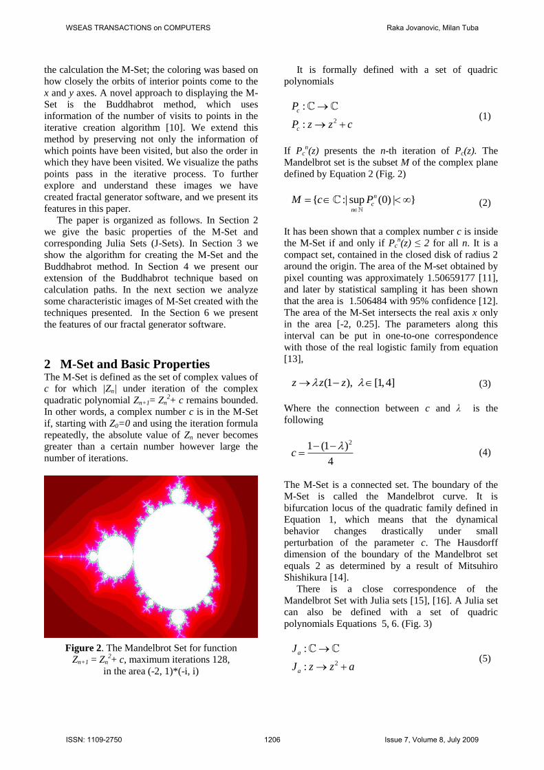
Figure 2. The Mandelbrot Set for function

Zn+1 = Zn2+ c, maximum iterations 128,

in the area (-2, 1)*(-i, i)

It is formally defined with a set of quadric

polynomials

2

:

:

c

c

P

P z z c

(1)

If Pcn(z) presents the n-th iteration of Pc(z). The

Mandelbrot set is the subset M of the complex plane

defined by Equation 2 (Fig. 2)

{ :| sup (0) | }n

cn

M c P

(2)

It has been shown that a complex number c is inside

the M-Set if and only if Pcn(z) ≤ 2 for all n. It is a

compact set, contained in the closed disk of radius 2

around the origin. The area of the M-set obtained by

pixel counting was approximately 1.50659177 [11],

and later by statistical sampling it has been shown

that the area is 1.506484 with 95% confidence [12].

The area of the M-Set intersects the real axis x only

in the area [-2, 0.25]. The parameters along this

interval can be put in one-to-one correspondence

with those of the real logistic family from equation

[13],

(1 ), [1,4]z z z (3)

Where the connection between c and λ is the

following

21 (1 )

4c

(4)

The M-Set is a connected set. The boundary of the

M-Set is called the Mandelbrot curve. It is

bifurcation locus of the quadratic family defined in

Equation 1, which means that the dynamical

behavior changes drastically under small

perturbation of the parameter c. The Hausdorff

dimension of the boundary of the Mandelbrot set

equals 2 as determined by a result of Mitsuhiro

Shishikura [14].

There is a close correspondence of the

Mandelbrot Set with Julia sets [15], [16]. A Julia set

can also be defined with a set of quadric

polynomials Equations 5, 6. (Fig. 3)

2

:

:

a

a

J

J z z a

(5)



{ :| sup ( ) | }n

a an

J z J z

(6)

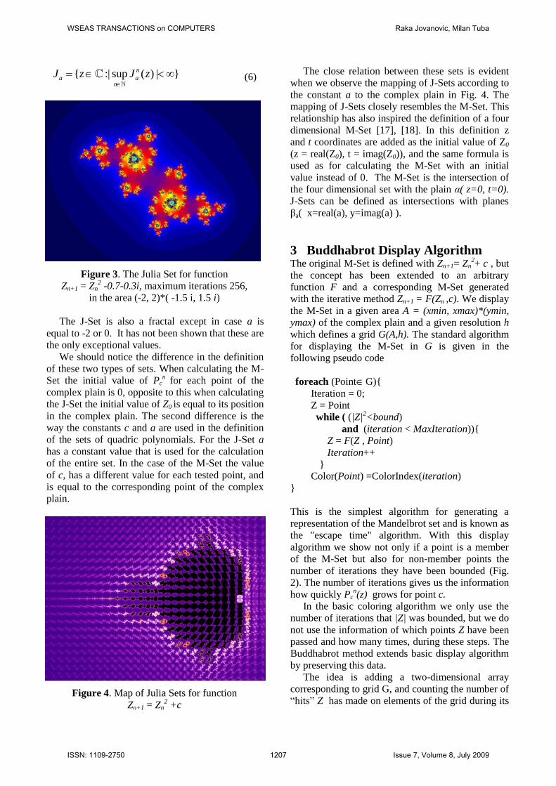
Figure 3. The Julia Set for function

Zn+1 = Zn2 -0.7-0.3i, maximum iterations 256,

in the area (-2, 2)*( -1.5 i, 1.5 i)

The J-Set is also a fractal except in case a is

equal to -2 or 0. It has not been shown that these are

the only exceptional values.

We should notice the difference in the definition

of these two types of sets. When calculating the M-

Set the initial value of Pcn

for each point of the

complex plain is 0, opposite to this when calculating

the J-Set the initial value of Z0 is equal to its position

in the complex plain. The second difference is the

way the constants c and a are used in the definition

of the sets of quadric polynomials. For the J-Set a

has a constant value that is used for the calculation

of the entire set. In the case of the M-Set the value

of c, has a different value for each tested point, and

is equal to the corresponding point of the complex

plain.

Figure 4. Map of Julia Sets for function

Zn+1 = Zn2 +c

The close relation between these sets is evident

when we observe the mapping of J-Sets according to

the constant a to the complex plain in Fig. 4. The

mapping of J-Sets closely resembles the M-Set. This

relationship has also inspired the definition of a four

dimensional M-Set [17], [18]. In this definition z

and t coordinates are added as the initial value of Z0

(z = real(Z0), t = imag(Z0)), and the same formula is

used as for calculating the M-Set with an initial

value instead of 0. The M-Set is the intersection of

the four dimensional set with the plain α( z=0, t=0).

J-Sets can be defined as intersections with planes

βa( x=real(a), y=imag(a) ).

3 Buddhabrot Display Algorithm The original M-Set is defined with Zn+1= Zn

2+ c , but

the concept has been extended to an arbitrary

function F and a corresponding M-Set generated

with the iterative method Zn+1 = F(Zn ,c). We display

the M-Set in a given area A = (xmin, xmax)*(ymin,

ymax) of the complex plain and a given resolution h

which defines a grid G(A,h). The standard algorithm

for displaying the M-Set in G is given in the

following pseudo code

foreach (PointG){

Iteration = 0;

Z = Point

while ( (|Z|2<bound)

and (iteration < MaxIteration)){

Z = F(Z , Point)

Iteration++

}

Color(Point) =ColorIndex(iteration)

}

This is the simplest algorithm for generating a

representation of the Mandelbrot set and is known as

the "escape time" algorithm. With this display

algorithm we show not only if a point is a member

of the M-Set but also for non-member points the

number of iterations they have been bounded (Fig.

2). The number of iterations gives us the information

how quickly Pcn(z) grows for point c.

In the basic coloring algorithm we only use the

number of iterations that |Z| was bounded, but we do

not use the information of which points Z have been

passed and how many times, during these steps. The

Buddhabrot method extends basic display algorithm

by preserving this data.

The idea is adding a two-dimensional array

corresponding to grid G, and counting the number of

“hits” Z has made on elements of the grid during its



iterations. The Buddhabrot algorithm is shown in the

following pseudo code.

Counter.SetToZero();

for (MaxNumberOfPoints){

Point = Random element of area A

Iteration = 0

Z = Point

Steps.Empty()

while ( (|Z|2<bound)

and (iteration < MaxIteration)){ Steps.Add(Z)

Z = F(Z , Point)

Iteration++

}

if((iteration=MaxIteration)=OUTSIDE){

foreach(Z Steps)

Counter (Z) += 1

}

}

foreach (PointG){

Color(Point) = ColorIndex(Counter(Point))

}

We wish to point out some differences compared to

the basic algorithm. First, instead of using the nodes

of the grid, we use a fixed number of random points

inside area A. This is important because if we took

just nodes of a square grid, a possibility exists that

they shall have some common properties and our

“statistical” image will not be correct in that case.

For each tested point we save the iteration steps in

an array Steps. This is done because we create two

separate images: one for points inside (Fig. 5), and

one for points outside (Fig. 6) the M-Set.

Figure 5. The Buddhabrot coloring, outside points,

maximum iterations 25600, points rendered 24*104

Counter is a two-dimensional array that corresponds

to blocks of grid G, it is used as the counter of

“hits”. After finishing the calculations loop for a

point, depending on whether it is a member of the

M-Set, we update the Counter with the points that

have been crossed. After MaxNumberOfPoints has

been reached we use the Counter for coloring the

screen. The image acquired with this algorithm for

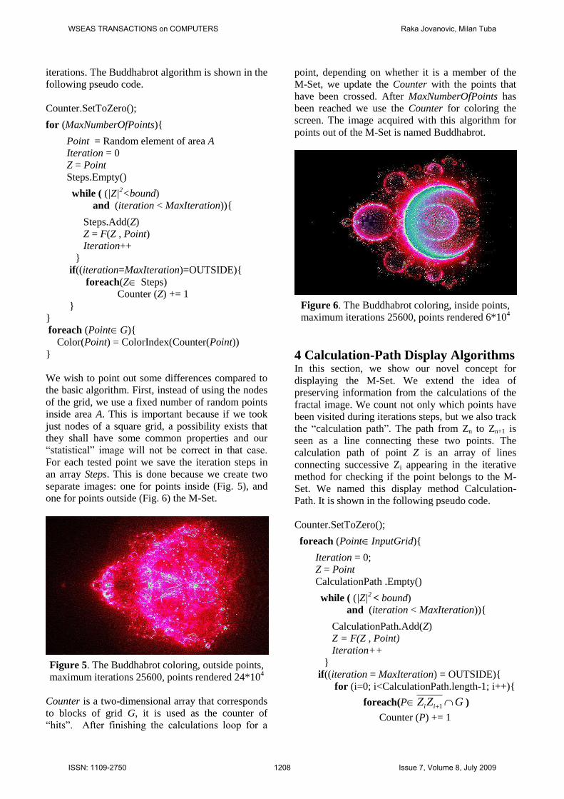
points out of the M-Set is named Buddhabrot.

Figure 6. The Buddhabrot coloring, inside points,

maximum iterations 25600, points rendered 6*104

4 Calculation-Path Display Algorithms In this section, we show our novel concept for

displaying the M-Set. We extend the idea of

preserving information from the calculations of the

fractal image. We count not only which points have

been visited during iterations steps, but we also track

the “calculation path”. The path from Zn to Zn+1 is

seen as a line connecting these two points. The

calculation path of point Z is an array of lines

connecting successive Zi appearing in the iterative

method for checking if the point belongs to the M-

Set. We named this display method Calculation-

Path. It is shown in the following pseudo code.

Counter.SetToZero();

foreach (PointInputGrid){

Iteration = 0;

Z = Point

CalculationPath .Empty()

while ( (|Z|2 < bound)

and (iteration < MaxIteration)){

CalculationPath.Add(Z)

Z = F(Z , Point)

Iteration++

}

if((iteration = MaxIteration) = OUTSIDE){

for (i=0; i<CalculationPath.length-1; i++){

foreach(P 1i iZ Z G )

Counter (P) += 1



}

}

}

foreach (PointG){

Color(Point) = ColorIndex(Counter(Point))

}

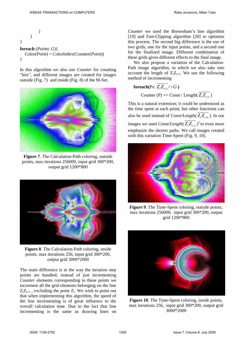
In this algorithm we also use Counter for counting

“hits”, and different images are created for images

outside (Fig. 7) and inside (Fig. 8) of the M-Set.

Figure 7. The Calculation-Path coloring, outside

points, max iterations 256000, input grid 300*200,

output grid 1200*800

Figure 8. The Calculation-Path coloring, inside



The main difference is in the way the iteration step

points are handled, instead of just incrementing

Counter elements corresponding to these points we

increment all the grid elements belonging on the line

ZiZi+1 , excluding the point Zi. We wish to point out

that when implementing this algorithm, the speed of

the line incrementing is of great influence to the

overall calculation time. Due to the fact that line

incrementing is the same as drawing lines on

Counter we used the Bresenham’s line algorithm

[19] and Fast-Clipping algorithm [20] to optimize

this process. The second big difference is the use of

two grids, one for the input points, and a second one

for the finalized image. Different combination of

these grids gives different effects to the final image.

We also propose a variation of the Calculation-

Path image algorithm, in which we also take into

account the length of ZiZi+1. We use the following

method of incrementing

foreach(P 1i iZ Z G )

Counter (P) += Const / Length( 1i iZ Z )

This is a natural extension; it could be understood as

the time spent at each point, but other functions can

also be used instead of Const/Length( 1i iZ Z ). In our

images we used Const/Length( 1i iZ Z )2 to even more

emphasize the shorter paths. We call images created

with this variation Time-Spent (Fig. 9, 10).

Figure 9. The Time-Spent coloring, outside points,

max iterations 256000, input grid 300*200, output

grid 1200*800

Figure 10. The Time-Spent coloring, inside points,

max iterations 256, input grid 300*200, output grid

3000*2000



5 Calculation-Path Fractal Images Due to the similarity of algorithms for generating the

BUD, CP and TS images we shall compare some of

their properties. We first notice that for CP and TS

images we need a lower number of points for

creating images due to the fact that we are drawing

lines instead of points. When generating images with

a large number of points, images can even lose

details due to intensive overlapping of paths. In this

case, more statistical information is presented, but

individual paths are less visible. When creating the

new type images, instead of using random points we

used points of a grid. This approach gave a more

representative sampling of the space when a small

number of points were tested. Images acquired when

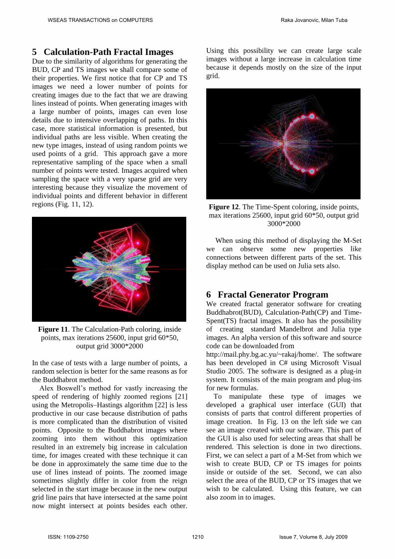
sampling the space with a very sparse grid are very

interesting because they visualize the movement of

individual points and different behavior in different

regions (Fig. 11, 12).

Figure 11. The Calculation-Path coloring, inside



In the case of tests with a large number of points, a

random selection is better for the same reasons as for

the Buddhabrot method.

Alex Boswell’s method for vastly increasing the

speed of rendering of highly zoomed regions [21]

using the Metropolis–Hastings algorithm [22] is less

productive in our case because distribution of paths

is more complicated than the distribution of visited

points. Opposite to the Buddhabrot images where

zooming into them without this optimization

resulted in an extremely big increase in calculation

time, for images created with these technique it can

be done in approximately the same time due to the

use of lines instead of points. The zoomed image

sometimes slightly differ in color from the reign

selected in the start image because in the new output

grid line pairs that have intersected at the same point

now might intersect at points besides each other.

Using this possibility we can create large scale

images without a large increase in calculation time

because it depends mostly on the size of the input

grid.

Figure 12. The Time-Spent coloring, inside points,

max iterations 25600, input grid 60*50, output grid

3000*2000

When using this method of displaying the M-Set

we can observe some new properties like

connections between different parts of the set. This

display method can be used on Julia sets also.

6 Fractal Generator Program We created fractal generator software for creating

Buddhabrot(BUD), Calculation-Path(CP) and Time-

Spent(TS) fractal images. It also has the possibility

of creating standard Mandelbrot and Julia type

images. An alpha version of this software and source

code can be downloaded from

http://mail.phy.bg.ac.yu/~rakaj/home/. The software

has been developed in C# using Microsoft Visual

Studio 2005. The software is designed as a plug-in

system. It consists of the main program and plug-ins

for new formulas.

To manipulate these type of images we

developed a graphical user interface (GUI) that

consists of parts that control different properties of

image creation. In Fig. 13 on the left side we can

see an image created with our software. This part of

the GUI is also used for selecting areas that shall be

rendered. This selection is done in two directions.

First, we can select a part of a M-Set from which we

wish to create BUD, CP or TS images for points

inside or outside of the set. Second, we can also

select the area of the BUD, CP or TS images that we

wish to be calculated. Using this feature, we can

also zoom in to images.



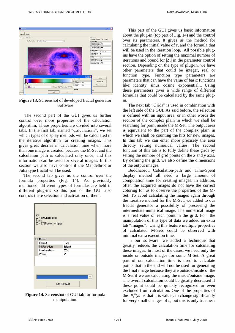
Figure 13. Screenshot of developed fractal generator

Software

The second part of the GUI gives us further

control over more properties of the calculation

algorithm. These properties are divided into several

tabs. In the first tab, named “Calculations”, we set

which types of display methods will be calculated in

the iterative algorithm for creating images. This

gives great decries in calculation time when more

than one image is created, because the M-Set and the

calculation path is calculated only once, and this

information can be used for several images. In this

section we also have control if the Mandelbrot or

Julia type fractal will be used.

The second tab gives us the control over the

formula properties (Fig. 14). As previously

mentioned, different types of formulas are held in

different plug-ins so this part of the GUI also

controls there selection and activation of them.

Figure 14. Screenshot of GUI tab for formula

manipulation.

This part of the GUI gives us basic information

about the plug-in (top part of Fig. 14) and the control

over its parameters. It gives us the method for

calculating the initial value of z, and the formula that

will be used in the iteration loop. All possible plug-

ins have the option of setting the maximal number of

iterations and bound for |Zn| in the parameter control

section. Depending on the type of plug-in, we have

other parameters that could be integer, real or

function type. Function type parameters are

parameters that can have the value of basic functions

like: identity, sinus, cosine, exponential... Using

these parameters gives a wide range of different

formulas that could be calculated by the same plug-

in.

The next tab “Grids” is used in combination with

the left side of the GUI. As said before, the selection

is defined with an input area, or in other words the

section of the complex plain in which we shall be

searching for point inside the M-Set. The output area

is equivalent to the part of the complex plain in

which we shall be counting the hits for new images.

In this tab we can enter more precisely the area

directly setting numerical values. The second

function of this tab is to fully define these grids by

setting the number of grid points on the x and y axis.

By defining the grid, we also define the dimensions

of the output images.

Buddhabrot, Calculation-path and Time-Spent

display method all need a large amount of

computation time for creating images. In addition,

often the acquired images do not have the correct

coloring for us to observe the properties of the M-

Set. To avoid calculating the images again through

the iterative method for the M-Set, we added to our

fractal generator a possibility of preserving the

intermediate numerical image. The numerical image

is a real value of each point in the grid. For the

manipulation of this type of data we added an extra

tab “Images”. Using this feature multiple properties

of calculated M-Sets could be observed with

minimal extra execution time.

In our software, we added a technique that

greatly reduces the calculation time for calculating

these images. In most of the cases, we need only the

inside or outside images for some M-Set. A great

part of our calculation time is used to calculate

points that in the end will not be used for generating

the final image because they are outside/inside of the

M-Set if we are calculating the inside/outside image.

The overall calculation could be greatly decreased if

these point could be quickly recognized or even

excluded from calculation. One of the properties of

the Pcn(z) is that it is value can change significantly

for very small changes of c, but this is only true near



the border of the M-Set. In areas not near the border

the behavior is stable. We used this property of the

M-Set to greatly optimize the calculation of BUD,

CP and TS large images, by developing an algorithm

that needs some assistance from the user.

The optimization has several steps. First, the user

calculates the image in some low resolution. Using

this image the user can select areas of the M-Set that

will be inside or outside of it depending on which

type of images while be calculated. The selection

consists of an array of rectangles with an

extra property that specifies if a point should be

inside or outside of it; an example of this selection

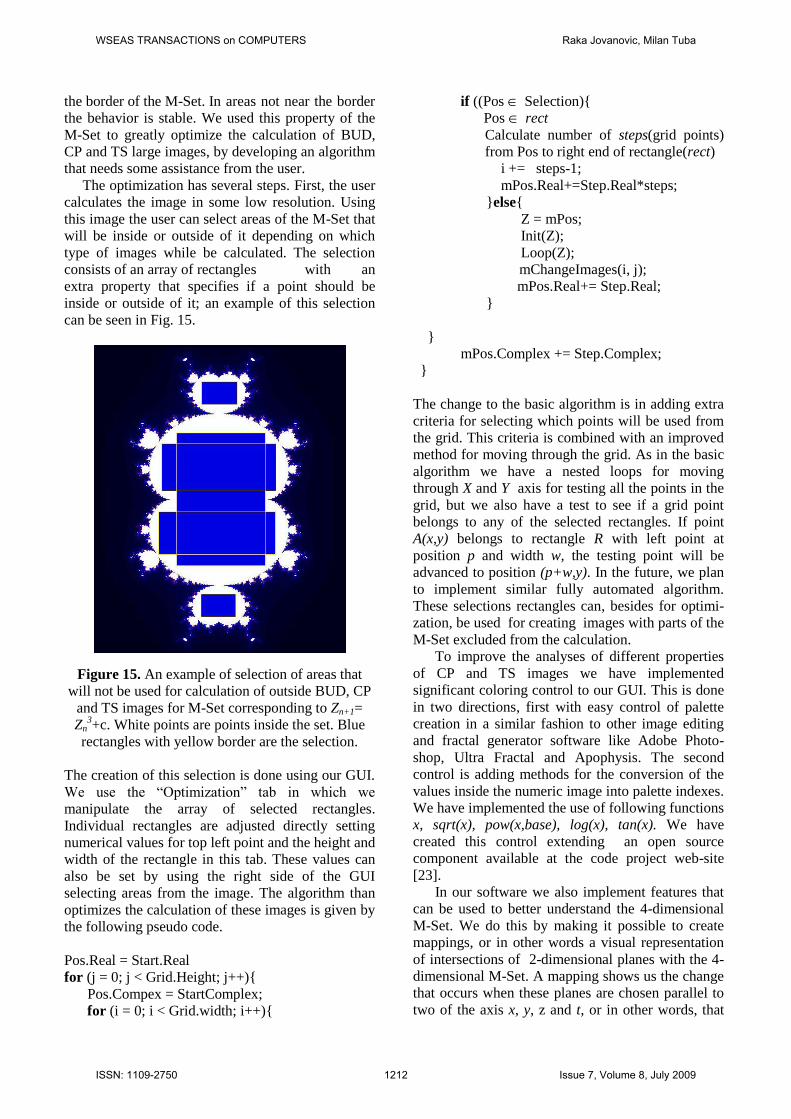
can be seen in Fig. 15.

Figure 15. An example of selection of areas that

will not be used for calculation of outside BUD, CP

and TS images for M-Set corresponding to Zn+1=

Zn3+c. White points are points inside the set. Blue

rectangles with yellow border are the selection.

The creation of this selection is done using our GUI.

We use the “Optimization” tab in which we

manipulate the array of selected rectangles.

Individual rectangles are adjusted directly setting

numerical values for top left point and the height and

width of the rectangle in this tab. These values can

also be set by using the right side of the GUI

selecting areas from the image. The algorithm than

optimizes the calculation of these images is given by

the following pseudo code.

Pos.Real = Start.Real

for (j = 0; j < Grid.Height; j++){

Pos.Compex = StartComplex;

for (i = 0; i < Grid.width; i++){

if ((Pos Selection){

Pos rect

Calculate number of steps(grid points)

from Pos to right end of rectangle(rect)

i += steps-1;

mPos.Real+=Step.Real*steps;

}else{

Z = mPos;

Init(Z);

Loop(Z);

mChangeImages(i, j);

mPos.Real+= Step.Real;

}

}

mPos.Complex += Step.Complex;

}

The change to the basic algorithm is in adding extra

criteria for selecting which points will be used from

the grid. This criteria is combined with an improved

method for moving through the grid. As in the basic

algorithm we have a nested loops for moving

through X and Y axis for testing all the points in the

grid, but we also have a test to see if a grid point

belongs to any of the selected rectangles. If point

A(x,y) belongs to rectangle R with left point at

position p and width w, the testing point will be

advanced to position (p+w,y). In the future, we plan

to implement similar fully automated algorithm.

These selections rectangles can, besides for optimi-

zation, be used for creating images with parts of the

M-Set excluded from the calculation.

To improve the analyses of different properties

of CP and TS images we have implemented

significant coloring control to our GUI. This is done

in two directions, first with easy control of palette

creation in a similar fashion to other image editing

and fractal generator software like Adobe Photo-

shop, Ultra Fractal and Apophysis. The second

control is adding methods for the conversion of the

values inside the numeric image into palette indexes.

We have implemented the use of following functions

x, sqrt(x), pow(x,base), log(x), tan(x). We have

created this control extending an open source

component available at the code project web-site

[23].

In our software we also implement features that

can be used to better understand the 4-dimensional

M-Set. We do this by making it possible to create

mappings, or in other words a visual representation

of intersections of 2-dimensional planes with the 4-

dimensional M-Set. A mapping shows us the change

that occurs when these planes are chosen parallel to

two of the axis x, y, z and t, or in other words, that



they can be defined with the following way α(

axis1=a, axis2=b). When creating a mapping

parameters a and b are selected on some uniform

grid for areas (A1, A2) and (B1, B2) This is better

understood if we observe Fig. 16, 17. In both of

these figures the center of the image corresponds to

the intersection with the plain that holds coordinate

center (0 + 0*i ) of the complex plane.

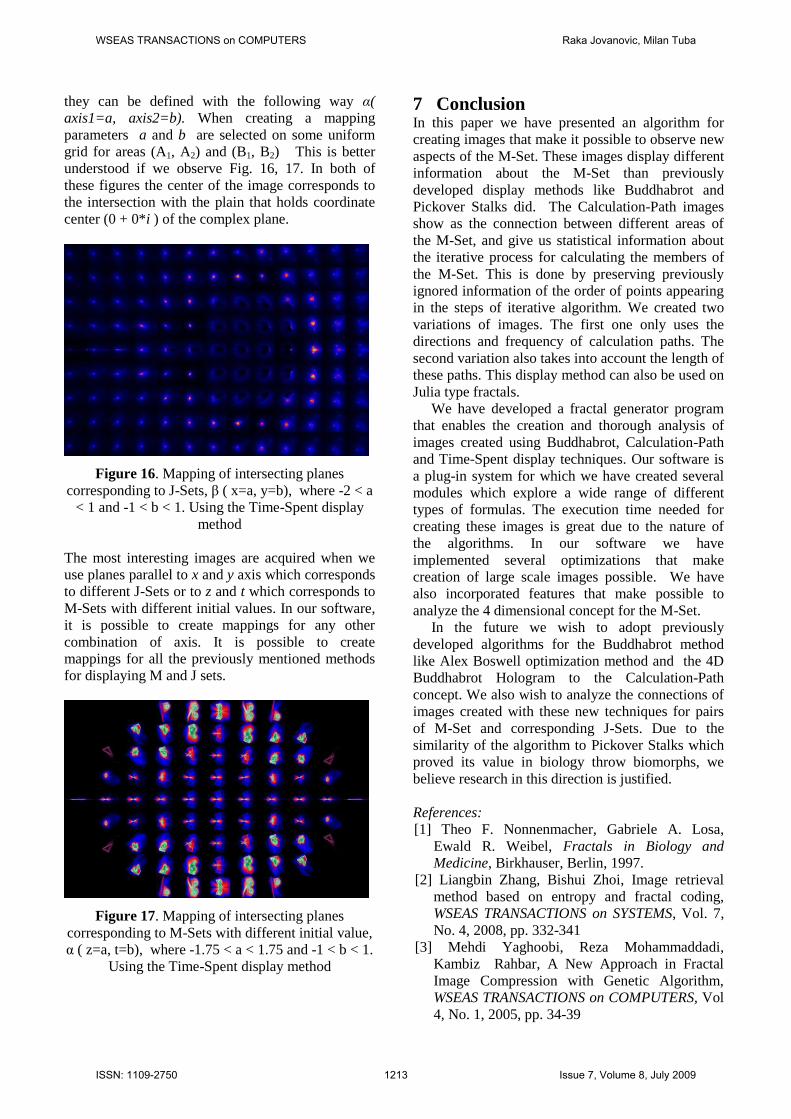
Figure 16. Mapping of intersecting planes

corresponding to J-Sets, β ( x=a, y=b), where -2 < a

< 1 and -1 < b < 1. Using the Time-Spent display

method

The most interesting images are acquired when we

use planes parallel to x and y axis which corresponds

to different J-Sets or to z and t which corresponds to

M-Sets with different initial values. In our software,

it is possible to create mappings for any other

combination of axis. It is possible to create

mappings for all the previously mentioned methods

for displaying M and J sets.

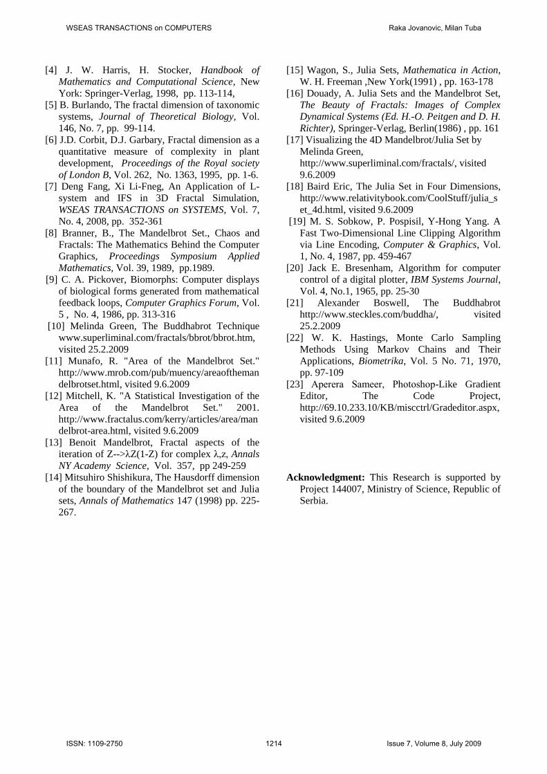
Figure 17. Mapping of intersecting planes

corresponding to M-Sets with different initial value,

α ( z=a, t=b), where -1.75 < a < 1.75 and -1 < b < 1.

Using the Time-Spent display method

7 Conclusion In this paper we have presented an algorithm for

creating images that make it possible to observe new

aspects of the M-Set. These images display different

information about the M-Set than previously

developed display methods like Buddhabrot and

Pickover Stalks did. The Calculation-Path images

show as the connection between different areas of

the M-Set, and give us statistical information about

the iterative process for calculating the members of

the M-Set. This is done by preserving previously

ignored information of the order of points appearing

in the steps of iterative algorithm. We created two

variations of images. The first one only uses the

directions and frequency of calculation paths. The

second variation also takes into account the length of

these paths. This display method can also be used on

Julia type fractals.

We have developed a fractal generator program

that enables the creation and thorough analysis of

images created using Buddhabrot, Calculation-Path

and Time-Spent display techniques. Our software is

a plug-in system for which we have created several

modules which explore a wide range of different

types of formulas. The execution time needed for

creating these images is great due to the nature of

the algorithms. In our software we have

implemented several optimizations that make

creation of large scale images possible. We have

also incorporated features that make possible to

analyze the 4 dimensional concept for the M-Set.

In the future we wish to adopt previously

developed algorithms for the Buddhabrot method

like Alex Boswell optimization method and the 4D

Buddhabrot Hologram to the Calculation-Path

concept. We also wish to analyze the connections of

images created with these new techniques for pairs

of M-Set and corresponding J-Sets. Due to the

similarity of the algorithm to Pickover Stalks which

proved its value in biology throw biomorphs, we

believe research in this direction is justified.

References:

[1] Theo F. Nonnenmacher, Gabriele A. Losa,

Ewald R. Weibel, Fractals in Biology and

Medicine, Birkhauser, Berlin, 1997.

[2] Liangbin Zhang, Bishui Zhoi, Image retrieval

method based on entropy and fractal coding,

WSEAS TRANSACTIONS on SYSTEMS, Vol. 7,

No. 4, 2008, pp. 332-341

[3] Mehdi Yaghoobi, Reza Mohammaddadi,

Kambiz Rahbar, A New Approach in Fractal

Image Compression with Genetic Algorithm,

WSEAS TRANSACTIONS on COMPUTERS, Vol

4, No. 1, 2005, pp. 34-39



[4] J. W. Harris, H. Stocker, Handbook of

Mathematics and Computational Science, New

York: Springer-Verlag, 1998, pp. 113-114,

[5] B. Burlando, The fractal dimension of taxonomic

systems, Journal of Theoretical Biology, Vol.

146, No. 7, pp. 99-114.

[6] J.D. Corbit, D.J. Garbary, Fractal dimension as a

quantitative measure of complexity in plant

development, Proceedings of the Royal society

of London B, Vol. 262, No. 1363, 1995, pp. 1-6.

[7] Deng Fang, Xi Li-Fneg, An Application of L-

system and IFS in 3D Fractal Simulation,

WSEAS TRANSACTIONS on SYSTEMS, Vol. 7,

No. 4, 2008, pp. 352-361

[8] Branner, B., The Mandelbrot Set., Chaos and

Fractals: The Mathematics Behind the Computer

Graphics, Proceedings Symposium Applied

Mathematics, Vol. 39, 1989, pp.1989.

[9] C. A. Pickover, Biomorphs: Computer displays

of biological forms generated from mathematical

feedback loops, Computer Graphics Forum, Vol.

5 , No. 4, 1986, pp. 313-316

[10] Melinda Green, The Buddhabrot Technique

www.superliminal.com/fractals/bbrot/bbrot.htm,

visited 25.2.2009

[11] Munafo, R. "Area of the Mandelbrot Set."

http://www.mrob.com/pub/muency/areaoftheman

delbrotset.html, visited 9.6.2009

[12] Mitchell, K. "A Statistical Investigation of the

Area of the Mandelbrot Set." 2001.

http://www.fractalus.com/kerry/articles/area/man

delbrot-area.html, visited 9.6.2009

[13] Benoit Mandelbrot, Fractal aspects of the

iteration of Z-->λZ(1-Z) for complex λ,z, Annals

NY Academy Science, Vol. 357, pp 249-259

[14] Mitsuhiro Shishikura, The Hausdorff dimension

of the boundary of the Mandelbrot set and Julia

sets, Annals of Mathematics 147 (1998) pp. 225-

267.

[15] Wagon, S., Julia Sets, Mathematica in Action,

W. H. Freeman ,New York(1991) , pp. 163-178

[16] Douady, A. Julia Sets and the Mandelbrot Set,

The Beauty of Fractals: Images of Complex

Dynamical Systems (Ed. H.-O. Peitgen and D. H.

Richter), Springer-Verlag, Berlin(1986) , pp. 161

[17] Visualizing the 4D Mandelbrot/Julia Set by

Melinda Green,

http://www.superliminal.com/fractals/, visited

9.6.2009

[18] Baird Eric, The Julia Set in Four Dimensions,

http://www.relativitybook.com/CoolStuff/julia_s

et_4d.html, visited 9.6.2009

[19] M. S. Sobkow, P. Pospisil, Y-Hong Yang. A

Fast Two-Dimensional Line Clipping Algorithm

via Line Encoding, Computer & Graphics, Vol.

1, No. 4, 1987, pp. 459-467

[20] Jack E. Bresenham, Algorithm for computer

control of a digital plotter, IBM Systems Journal,

Vol. 4, No.1, 1965, pp. 25-30

[21] Alexander Boswell, The Buddhabrot

http://www.steckles.com/buddha/, visited

25.2.2009

[22] W. K. Hastings, Monte Carlo Sampling

Methods Using Markov Chains and Their

Applications, Biometrika, Vol. 5 No. 71, 1970,

pp. 97-109

[23] Αperera Sameer, Photoshop-Like Gradient

Editor, The Code Project,

http://69.10.233.10/KB/miscctrl/Gradeditor.aspx,

visited 9.6.2009

Acknowledgment: This Research is supported by

Project 144007, Ministry of Science, Republic of

Serbia.



A Visual Αnalysis of Calculation-Paths of the …...application and use of fractals has been...

Documents

Transcript of A Visual Αnalysis of Calculation-Paths of the …...application and use of fractals has been...