A new Bismut-Elworthy-Li-formulafor diffusions with singular coefficientsdriven by a pure jump Levy process

and applications to life insurance

by

Tor Martin Christensen

Thesis

for the degree of

Master of science

(Master i Modellering og Dataanalyse)

Faculty of Mathematics and Natural Sciences

University of Oslo

April 2015

Det matematisk- naturvitenskapelige fakultetUniversitetet i Oslo

Abstract

The main result of my mine in the master thesis is a new Bismut-Elworthy-Li-formula with respect to a pure jump Levy noise driven stochastic differentialequation (SDE), with non-Lipschitz continuous coefficients. More precisely,I obtain in this thesis for the first time the following representation:

∂

∂xE[g(Xx

T )] = E

[g(Xx

T ) · 1

Sα/2T

∫ T

0

∂

∂xXxs dLs

],

where g is a continuous function and where Xxt satisfies the SDE

Xxt = x+

∫ t

0

b(Xxs )ds+ Lt, 0 ≤ t ≤ T

for an α-stable process Lt, α ∈ (1, 2) and a α2-stable subordinator S

α/2t . Here

we only require that the drift coefficient is Holder continuous. We mentionthat the above result, which is a generalization of the paper [17] to the caseof singular drift coefficients b, was first obtained in [12] for SDE’s driven byBrownian motion.

Let me also remark that the above formula can be considered a repre-sentation of ”pure jump Levy” delta of a financial claim h = g(Xx

T ) with anunderlying asset price dynamics given by Xs, 0 ≤ s ≤ T , which does notinvolve a derivative of the payoff function g.

This thesis consists of 5 chapters, where chapter 1 is an introduction towhat Greeks are and why they are interesting in finance. In chapter 2 thereis an overview and discussion of basic methods for the calculation of Greeksin the literature. In chapter 3 there is an implementation of what we referto as Zhang’s formula, namely a Bismut-Elworthy-Li type formula. This is a”derivative free” type formula for SDEs driven by pure jump process, namelyan α-stable process. In the first part of chapter 3 simulations are conductedconfirming that Zhang formula in numerical implementations works, thenthere is presented an application of this formula to life insurance, where wealso conduct simulations.

Chapter 4 is the highlight of this thesis, where we derive a Bismut-Elworthy-Li type formula for the Greek Delta. This derivative free repre-sentation is obtained by using methods in [17] and [8]. The formula can beregarded as an extension of Zhang’s formula in case of the Greek Delta, inthe sense that we deal with Holder coefficients and don’t demand that thecoefficients have continuous first order derivative.

Chapter 5 suggests possible extensions to this thesis.

i

Acknowledgements

I would like to thank my supervisor Frank Proske, for providing me with achallenging and very interesting topic for my thesis, along with his help andguidance.

I want to thank my parents Tor and Mette for their support during mystudies. I would like to thank my fellow students at room 802 for an enjoy-able working environment these past two years. I want to thank Maja, andespecially Lars for interesting discussions and finding misprints. I would liketo thank family and friends for encouragement, especially Jonas Skaalen.

And last but not least my girlfriend, Marte, for all her love and invaluablesupport.

iii

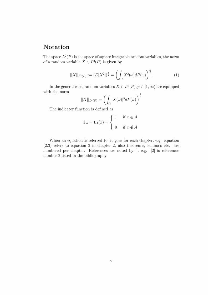
Notation

The space L2(P ) is the space of square integrable random variables, the normof a random variable X ∈ L2(P ) is given by

||X||L2(P ) := (E[X2])12 =

(∫Ω

X2(ω)dP (ω)

) 12

. (1)

In the general case, random variables X ∈ Lp(P ), p ∈ [1,∞) are equippedwith the norm

||X||Lp(P ) =

(∫Ω

|X(ω)|pdP (ω)

) 1p

The indicator function is defined as

1A = 1A(x) =

1 if x ∈ A

0 if x /∈ A

When an equation is referred to, it goes for each chapter, e.g. equation(2.3) refers to equation 3 in chapter 2, also theorem’s, lemma’s etc. arenumbered per chapter. References are noted by [], e.g. [2] is referencesnumber 2 listed in the bibliography.

v

Contents

Preface i

Abstract . . . . . . . . . . . . . . . . . . . . . . . . . . . . . . . . . i

Acknowledgements . . . . . . . . . . . . . . . . . . . . . . . . . . . iii

Notation . . . . . . . . . . . . . . . . . . . . . . . . . . . . . . . . . v

1 Introduction 1

2 Overview of basic methods for calculation of Greeks 5

2.1 Overview of numerical techniques for computations of Greeks . 6

2.1.1 The finite difference method . . . . . . . . . . . . . . . 9

2.1.2 Numerical method through Malliavin Calculus . . . . . 10

2.1.3 The Likelihood Ratio Method . . . . . . . . . . . . . . 12

2.2 Overview of concepts in Malliavin calculus in case of the Brow-nian motion . . . . . . . . . . . . . . . . . . . . . . . . . . . . 13

2.3 Malliavin calculus in case of Levy processes . . . . . . . . . . 19

3 Implementation of Greeks driven by α-stable processes 23

3.1 Levy processes . . . . . . . . . . . . . . . . . . . . . . . . . . . 25

3.2 Modeling with the α-stable processes . . . . . . . . . . . . . . 29

3.3 Derivative formula and gradients estimates for SDE’s . . . . . 33

3.4 Simulation of the derivative of a caplet with respect to theinitial interest rate, under the Vasicek interest rate model . . . 35

3.4.1 The Vasicek interest rate model . . . . . . . . . . . . . 35

3.4.2 Simulation of the derivative of a caplet with respect tothe initial interest rate . . . . . . . . . . . . . . . . . . 38

3.5 Application to life insurance . . . . . . . . . . . . . . . . . . . 42

3.5.1 Framework in life insurance . . . . . . . . . . . . . . . 43

3.5.2 Unit-linked policies . . . . . . . . . . . . . . . . . . . . 46

3.5.3 Simulation of the sensitivity of unit-linked policies . . . 48

vii

4 Derivation of the delta in the case of SDE’s with Holder driftcoefficients 554.1 Framework . . . . . . . . . . . . . . . . . . . . . . . . . . . . . 564.2 Properties of an SDE with Holder coefficients . . . . . . . . . 604.3 A Bismut-Elworthy-Li formula (”delta”) with Holder coefficients 66

5 Extensions 73

A Appendix 75A.1 Calculations . . . . . . . . . . . . . . . . . . . . . . . . . . . . 75A.2 R-code for simulations . . . . . . . . . . . . . . . . . . . . . . 78A.3 Bibliography . . . . . . . . . . . . . . . . . . . . . . . . . . . . 104

viii

Chapter 1

Introduction

In the world of finance, there are numerous types of contracts often knownas financial derivatives. The price of such contracts are derived from theunderlying asset, e.g. stocks, bonds, interest rates, currencies. A well knowntype of contract is the European call option. More precisely let S(T ) denotethe value of the underlying asset, where T is the time to maturity, thatis, when the option can be exercised. Furthermore, if K denotes the strikeprice, the option takes the form max(S(T )−K, 0), where the investor paysan agreed upon sum to the other party when the contract starts. This givesthe investor the right to purchase the underlying asset at a price in the futureagreed upon today. Such contracts can be used as an insurance, in the sensethat an investor can buy protection if the value of the underlying asset theinvestor holds crosses a threshold. This strategy is a type of hedge, that is toreduce the risk. A highly interesting topic is how sensitive they are when aparameter changes, maybe the underlying asset becomes more volatile or thedrift changes. What if the value of the underlying asset changes? This branchof financial mathematics is known as sensitivity analysis or more commonlyreferred to as Greeks. This tool is often applied by investors in the financialmarket, as risk measure, used to hedge their positions.

When one computes Greeks in finance, one investigates the market sen-sitivities of financial derivatives (e.g. call option, put option, digital optionetc.) when parameters in a given model change. These quantities are of-ten denoted by Greek letters, hence the name Greeks. To obtain a Greekthe main idea is to take the derivative of the risk-neutral price of an option(e.g. call option) with respect to the parameter one is interested in. Moreprecisely, if we let

V = EQ[e−∫ T0 r(s)dsφ(S(T ))]

denote the risk-neutral price, where φ denotes the payout function, S(T ) the

1

value of the underlying asset (e.g. a stock) at terminal time T . Furthermore

r denotes the overnight interest rate (so e−∫ T0 r(s)ds is the discount factor), and

the expectation is taken with respect to the risk neutral probability measureQ. To obtain a Greek, one must take the partial derivative of a parameterof the risk-neutral price, e.g.:

Delta is used to construct the delta hedge in a portfolio, denoted ∆ =∂V∂x

. Delta measures the sensitivity of change in the price x of theunderlying asset. In fact taking the derivative with respect to theunderlying asset gives us the hedge ratio, which is needed to obtain thereplicating portfolio.

Gamma is the derivative of the delta with respect to the price x of theunderlying asset, Γ = ∂2V

∂x2.

Rho measures the sensitivity to the interest rate, which is obtained bytaking the derivative with respect to r, ρ = ∂V

∂r.

Theta is obtained by taking the derivative with respect to time: θ =−∂V∂T

, theta measures the sensitivity to the time to maturity.

Vega, which is not a greek letter (but denoted by the Greek letter ν),measures sensitivity of V , with respect to the volatility of the underly-ing asset: ν = ∂V

∂σ.

These are some of the most common Greeks, but the possibilities areendless. Where the latter statement entails that one can find high order ofGreeks, that is, to take higher order derivatives of a risk-neutral price (V).We will consider first order Greeks in this thesis. Delta is a very interest-ing Greek, it is used to obtain the hedge ratio, which is needed to find thereplicating portfolio of a financial derivative, such as the call option. Wherethe replicating portfolio of an option is the portfolio strategy needed to pro-duce the same outcome as the option. In a replicating portfolio of an option,one invest in the underlying asset of the option and the bank. Taking thederivative of a risk-neutral price to e.g. obtain one of the Greeks above, canbe accomplished in a straight forward manner under nice conditions, that iswhen one is allowed to commute differentiation and expectation. Under theassumptions of a Black-Scholes model Greeks are relatively straight forwardto compute.

However, in general it is often impossible to obtain an analytical expres-sion for a Greek. Hence one would resort to numerical methods to obtainthe Greek that one sets out to find. For instance, if the payout function

2

is discontinuous it may be impossible to obtain the derivative. One couldresort to the so-called density method, where one moves the derivative ofthe payout function to only depend on the density function 1. This methodworks well, but one is required to have an explicit expression of the densityfunction. In fact it turns out that this method is a special case of the gen-eral Malliavin approach. With tools from Malliavin calculus, it is possible toobtain a derivative free form of Greeks by

EQ[e−∫ T0 r(s)dsφ(S(T ))π] (1.1)

where π is the so-called Malliavin weight. This was done by the authors in[6].

First we will look into the Malliavin weight π. To make this technique lessmysterious we include an overview of some important concepts of Malliavincalculus in the continuous case, namely Brownian motion. Readers familiarwith basic methods for numerical approximation of Greeks, such as finitedifference, likelihood ratio method and the application of Malliavin calculus,may skip chapter 2.

After an overview of basic methods to obtain Greeks we will introducethe concept of Levy processes. We look at Levy processes or more preciselypure jump processes, as a model able to capture jumps is considered morerealistic, e.g. if there is an abrupt change in a country’s monetary policy. Infact, we will study pure jump processes, that is, we assume that the processonly consists of jumps. More precisely we will work with the α-stable process,which is explained in chapter 3. With help from a Bismut-Elworthy-Li typeformula developed in [17] we will simulate/approximate Greeks, ran by α-stable processes.

1See the section about the Likelihood Ratio Method for details on this technique.

3

4

Chapter 2

Overview of basic methods for

calculation of Greeks

Obtaining Greeks analytically under a framework of differentiable payofffunctions and continuous process can be a straight forward process. Whenwe have nice conditions that allows us to commute differentiation and expec-tation. On the other hand, it can be quite challenging in certain scenarios,where one has to deal with jump processes, non-differentiable payoff functionsor very complicated options. One can approximate solutions numerically byvarious techniques, using Monte Carlo simulation, which we will see can beused to obtain quite accurate estimates. In this chapter we will first getan overview of techniques used to obtain Greeks numerically, where the ap-plication from Malliavin calculus is included. Furthermore because of theMalliavin weight π there is included an overview of some important conceptsin Malliavin calculus.

We will frequently encounter the stochastic process Brownian motionthroughout this thesis, which has the properties:

Definition 2.1. The Brownian motion B(t) is a continuous 1 stochastic

process which have the following properties

i) Independent increments: The random variable B(t)−B(s) is indepen-

dent of the random variable B(u)−B(v) where t > s ≥ u > v ≥ 0.

ii) Normal increments: The distribution of B(t) − B(s) for t > s ≥ 0 is

normal with expectation 0 and variance t− s.1But nowhere differentiable.

5

Also, we have the definition of what a σ-algebra is, which we will en-counter throughout the thesis. We will use Ft as the smallest σ-algebragenerated by the Brownian motion up to time t.

Definition 2.2. If Ω is a given set, then a σ-algebra F on Ω is a family F

of subsets of Ω with the following properties:

(i) ∅ ∈ F

(ii) F ∈ F ⇒ FC ∈ F , where FC = Ω\F is the complement of F in Ω

(iii) A1, A2, ... ∈ F ⇒ A := ∪∞i=1Ai ∈ F

2.1 Overview of numerical techniques for com-

putations of Greeks

If we assume that we have an underlying asset described by the stochasticdifferential equation (SDE)

dX(t) = b(X(t))dt+ σ(X(t))dB(t), (2.1)

where the coefficients b and σ are Lipschitz continuous, i.e. satisfies the usualconditions to make sure that the solution of eq. (2.1) exist and is unique 2.Furthermore B(t), 0 ≤ t ≤ T is the Brownian motion with values in Rn.Then the solution X(t); 0 ≤ t ≤ T is a Markov process with values in Rn.Let

u(x) = E[φ(X(T ))|X(0) = x], (2.2)

where T is the maturity time of an option and φ is the payoff function, e.g.call option, digital option, Asian option. The function u(x) denotes the priceof the option (with interest rate r = 0), which can be computed by MonteCarlo methods. One can investigate how sensitive an option is with respectto its different parameters. One needs to compute the differentials of u(x)with respect to the parameters one is interested in, e.g. the drift coefficientb, the volatility σ or the initial value x. Finding Greeks analytically maysometimes be impossible, thus one needs to resort to numerical methods. Tobe able to understand the numerical methods, in the next subsections, wewill first see how to simulate an expectation and an arbitrary dynamics ofthe form (2.1)

2See theorem 5.2.1 in [4] for details on the conditions concerning existence and unique-

ness of SDE’s.

6

The approximation in the Monte Carlo simulation is found by comput-ing the payoff function m times, and weighting each simulation equally. Theestimate for the expectation becomes more accurate as the number of simula-tions increases. As an example of a process of type (2.1), take the geometricBrownian motion, which is described by the dynamic

dX(t) = µX(t)dt+ σX(t)dBt (2.3)

for given constant drift and volatility respectively denoted by µ, σ ∈ R. Thesolution of the dynamic takes the form (proof is given in Lemma A.2)

Xt = x · exp

((µ− 1

2σ2)t+ σBt

), x = X(0), (2.4)

which can be obtained by using the Ito formula on eq. (2.3). If one were toapply this in practice, e.g. take the derivative with respect to the underlyingasset (obtain the hedge ratio), then one need to apply Girsanov’s theorem,to make sure that the process is risk neutral, so there are no arbitrage op-portunities 3.

If we want to approximate eq.(2.2) numerically, where we let XT be thegeometric Brownian motion, i.e. eq.(2.4).

The process varies in the sense that we need to simulate a new Bt foreach run, which will yield a different path for each simulation. This is em-phasized by the subscript j in eq. (2.7). First one need the simulations ofXt, which can be found recursively; for n ∈ N let 0 = t0 ≤ ... ≤ tn = T beuniformly distributed, so that the n time points have the same distance be-tween them, denoted by ∆t which becomes ∆t = T

n. Then we can simulate

Bt = (Bt0 , Bt1 , ..., Btn) by drawing N(0,∆t) (N(µ, σ2) denotes the normaldistribution with expectation µ and variance σ2) as follows:

Bt0 = Y0

Bt1 = Bt0 + Y1

Bt2 = Bt1 + Y2

...

Btn = Btn−1 + Yn

Where Y0, Y1, ..., Yn are i.i.d N(0,∆t). Utilizing this and starting the recur-

3For more about risk neutrality see [1].

7

sion at the point Xt0 = x we get the following:

Xtn = Xtn−1 · exp

((µ− 1

2σ2)∆t+ σ(Btn −Btn−1)

)(2.5)

= x · exp

((µ− 1

2σ2)T + σBtn

), (2.6)

where µ and σ are given constants, and x is the initial value of the underlyingasset. We see that the geometric Brownian motion has the Markov property,which simplifies computation; thus, conducting a numerical simulation on acomputer, eq. (2.6) is preferable to eq. (2.5) as this does not require anylooping. Furthermore, one needs to simulate an expectation, which we willdo by weighting each simulation equally, so we obtain the average, hence weneed to simulate equation (2.6) m times. We let the simulations (end pointof each recursion) be put into one vector, more precisely we let

X = (X1(T ), X2(T ), ..., Xm(T ))

denote the m simulations, where 4 Xj is an arbitrary simulation (1 ≤ j ≤ m)We can then use the following approximation:

u(x) = E[φ(X(T ))] ≈ 1

m

m∑j=1

φ(Xj(T )). (2.7)

where m is the number of simulations, higher values of m yields a moreaccurate value for the expectation. Since equation (2.7) is an approximationone need to consider the trade-off between increasing the accuracy for theexpectation and the computation time, when conducting simulations.

If one encounter a complex dynamic, which can be hard or even impossi-ble to solve analytically, one can solve the problem numerically. A straightforward approximation is the Euler scheme. More precisely, if one has ageneral dynamic of the form

dX(t) = b(X(t))dt+ σ(X(t))dB(t)

(as earlier), then one can utilize the following approximation to find a real-ization of X(T ) numerically:

4The parameters of the process Xj are suppressed, so when we use an illustrating

example later on, where we take the derivative with respect to a arbitrary parameter, it’s

assumed that the process is a function of that parameter.

8

Let 0 = t0 ≤ ... ≤ tn = T be uniformly distributed, so that the n timepoints have the same distance between them. Thus ∆t = T

n.

For 0 ≤ i ≤ n simulate the recursion

Xi+1 = b(Xi)∆t+ σ(Xi)∆Bi,

where X0 = x and

∆Bi = Bti+1−Bti .

2.1.1 The finite difference method

A basic method for computing the sensitivity of an option, e.g. delta, gamma,rho, is to deploy the finite difference method, which is based on finding anapproximation of the derivative numerically. If we for instance look at theDelta, one first have to use Monte Carlo to obtain an estimate of eq. (2.2)and an estimate for u(x + ε) for a small ε > 0. Using the forward finitedifference estimator, one gets the estimate

∆ =∂u(x)

∂x≈ u(x+ ε)− u(x)

ε. (2.8)

Alternatively, one can use the central difference method to obtain an evenbetter approximation:

∆ =∂u(x)

∂x≈ u(x+ ε)− u(x− ε)

2ε. (2.9)

With this method we get a faster rate of convergence.In fact we can use eq.(2.9) once more to obtain an approximation for the

Gamma:

Γ =∂2u(x)

∂x2≈ u(x+ ε?)− 2u(x) + u(x− ε?)

ε?2(2.10)

where 5 ε? = 2ε. One could argue here that since we pick an arbitrary ε, that2ε can easily be replaced by a new ε since all we demand is that ε > 0. Thereason why we use ε? is because of the choice of ε in eq. (2.9) and eq. (2.10)isn’t necessarily the same. The choice of ε can’t be too big or too small 6.Preferably one should use an equation which can provide us with the optimalchoice of ε. For the choice of ε in the case of Gamma see eq.(11.8) in [10].

5See lemma A.4 on the derivation of the Gamma approximation.6For a details on this topic see e.g. [10] page 141.

9

Approximation with Monte Carlo makes the central difference method,in the case of the delta take the form

∆ ≈ 1

2mε

m∑j=1

[φ(Xj(x+ ε))− φ(Xj(x− ε))]. (2.11)

The numerical approximation for Gamma takes the form

Γ ≈ 1

mε?2

m∑j=1

[φ(Xj(x+ ε?))− 2 · φ(Xj(x)) + φ(Xj(x− ε?))] (2.12)

It’s been proved (see [6]) that the convergence rate of the forward finitedifference estimator 7 is n−1/4. By using the central difference estimator, onehas a convergence rate of n−1/3, which significantly decrease the computa-tion time. It’s even possible to obtain a convergence rate of n−1/2 if one usecommon random numbers (a variance reduction technique) for both estima-tors. A drawback of the finite difference method is that it lacks the ability todeal with non-differentiable payoff functions, such as the digital option whichpays zero or one: φ(X(T )) = 1X(T )>K (where K denotes the strike priceof the option). By means of Malliavin calculus one can overcome this obsta-cle, namely be able to approximate a Greek that has a discontinuous payofffunction. In fact the method in the next subsection can also be deployed ifone has to deal with a Levy process, that is, when we allow for jumps in astochastic process.

2.1.2 Numerical method through Malliavin Calculus

An important application from Malliavin Calculus is that one can obtainclosed theoretical formulas for Greeks, where the differentiation operator is”moved away” from the payoff function. This method has the ability todeal with jump and continuous processes, where we don’t need to know theexplicit density 8. These formulas might be theoretically difficult to solve,but by deploying Monte Carlo simulation it’s possible to obtain accurateapproximations of Greeks. More precisely, a numerical approximation usingMalliavin calculus in combination with Monte Carlo yields a convergence

7Under the assumption that both estimators are drawn independently of each other in

the Monte Carlo simulation.8If one do however have the explicit density the Malliavin weight is easy to find, as

this mean we are essentially using the likelihood ratio method, as we shall see in the

forthcoming subsection.

10

rate of n−1/2. As shown by Fournie et al. in [6] by using Malliavin calculusone can express Greeks in the following way:

E[πφ(X(T ))|X(0) = x],

where π is the Malliavin weight. An important feature here is that π doesnot depend on the payoff function φ. The authors in [6] conducted numericalexperiments showing how well this works and compared it with the finitedifference method. This was done in a setting where they already knew thetheoretical values of a given Greek. Their numerical experiments showedthat this application of Malliavin calculus is very useful to compute Greeks.Note that the weights used were not unique. In the first paper they chosearbitrary non-complicated weights, where they in a follow up paper, namely[7] discuss the choice of the optimal Malliavin weight. They investigate theoptimal choice of weight in the sense of minimal variance. More precisely,for all possible weights π the idea is to minimize

V (π) = E[|φ(X(T ))π − d

dθu(x)|2]

= E[φ2(X(T ))π2]− E[φ(X(T ))π0]2

= E[φ2(X(T ))(π2 − π20)] + V (π0)

where π0 is the weight with the smallest variance and θ is an arbitrary pa-rameter that the risk-neutral price u(x) depend on.

The method of using the so-called Malliavin weight works well in thecase of discontinuous payoff functions, but for some Greeks the computationmight be slow e.g. if one has powers of the Brownian motion. 9

Usually the finite difference method performs just as good as deployingMalliavin calculus, except when we for instance deal with non-smooth pay-off functions. Thus in some cases, it’s more favorable to deploy the finitedifference method (depending on the payoff function) because it’s more cum-bersome to use Malliavin calculus in this case, as it requires that we set ofheavy theoretical machinery. Note that a downside of estimation by means ofMonte Carlo, is that it might converge slowly, and in some cases the estimatemight be poor.

9The authors of [6] point out that some weights may have powers of the Brownian

motion, which slows down the Monte Carlo simulations, so they introduce the idea of

what they call a localized version, to improve numerical simulations. For more on this

consult [6].

11

2.1.3 The Likelihood Ratio Method

The likelihood ratio method is a special case of an application of Malliavincalculus. Given that we are able to obtain the explicit density function(which must depend on the parameter we are differentiating with respect to)for the payoff function φ(X(T )), one can move the differentiation operatorinside the expectation. Thus we can move the dependence from the payofffunction to the density function, which makes us able to treat non-smoothpayoff functions. Letting the risk-neutral price of the option be on the formu(x) = E[φ(X(T ))|X(0) = x], where φ(X(T )) denotes the payoff function.We can observe how one can move the differentiation to only depend on thedensity function of the payoff function:

∂

∂zE[φ(X(T ))] =

∂

∂z

∫φ(y)fz(y)dy

=

∫φ(y)

∂

∂zfz(y)dy

=

∫φ(y)

∂

∂zfz(y) · fz(y)

fz(y)dy

=

∫ (φ(y)

∂

∂zlog(fz(y))

)fz(y)dy

= E[φ(X(T ))∂

∂zlog(fz(y))]

where z is some arbitrary parameter that our payoff function depend on, andfz(y) denotes the density function of the payoff function. The name of thismethod originates from the fact that the term

∂∂zfz(y)

fz(y)=

∂

∂zlog(fz(y))

in the above equality, could be regarded as a likelihood ratio in the sensethat its the ratio between two density functions. Computing the Delta (donein [10]) by means of Monte Carlo, in the case of the likelihood ratio methodone obtains the approximation

∆ ≈ 1

m

m∑j=1

[φ(Xj(T )) · ∂∂z

log(fz(φ(Xj(T )))]

where we simulate m times in order to compute the expectation.

12

2.2 Overview of concepts in Malliavin calcu-

lus in case of the Brownian motion

In the following section we will look at basic concepts of Malliavin calculusas it is presented by the authors in [4]. This will make us more familiarwith the Malliavin weight π. Malliavin calculus was introduced by PaulMalliavin, and was used as a tool to study the smoothness of densities ofsolutions of stochastic differential equations driven by Brownian motion. Atfirst this calculus was considered complicated with limited applications, butit soon became clear that Malliavin calculus was significant, due to appli-cations discovered in stochastic control, insider trading and the applicationin sensitivity analysis. The application in sensitivity analysis was discoveredby Fournie et al. ([6]), where they were able to move the derivative fromthe payoff function, which means one can treat a great deal of complicatedoptions (which could be non-differentiable). The so-called Malliavin weightπ is what we shall embark on in the following section. Here we will get anoverview of some of the important concepts used in the derivation of theweight π.

The Wiener-Ito chaos expansion

The weight π is defined through the Malliavin derivative, which is defined

through the Wiener-Ito chaos expansion. We first need the notion of the n-

fold iterated Ito integral, in which the Wiener-Ito chaos expansion is defined

through. Let B(t) = B(ω, t) (B(0) = 0), ω ∈ Ω, t ∈ [0, T ] (T > 0) be

the Brownian motion on the complete probability space (Ω,F , P ). Also we

denote by Ft the σ-algebra generated by B(s), 0 ≤ s ≤ t. We have the

following definition of a symmetric function:

Definition 2.3. A real function g : [0, T ]n −→ R is called symmetric if

g(tσ1,...,tσn ) = g(t1, ..., tn)

for all permutations σ = (σ1, ..., σn)of(1, 2, ..., n)

The symmetrization f of a real function f on [0, T ]n is defined by

f(t1, ...tn) =1

n!

∑σ

f(tσ1 , ..., tσn)

where we take the sum over all permutations of σ. Furthermore, we will work

in the space of square integrable Borel real functions on [0, T ]n denoted by

13

L2([0, T ]n), where the norm is defined as

||g||2L2([0,T ]n) =

∫[0,T ]n

g2(t1, ..., tn)dt1 · · · dtn <∞ (2.13)

Let L2([0, T ]n) denote the space of symmetric square integrable functions on

[0, T ]n, which is a subspace of L2([0, T ]n).

Let Sn = (t1, ..., tn) ∈ [0, T ]n : 0 ≤ t1 ≤ t2 ≤ ... ≤ tn ≤ T. Then we

have the following definition of the n-fold iterated Ito integral:

Definition 2.4. Let f be a deterministic function defined on Sn(n ≥ 1) such

that

||f ||2L2(Sn) :=

∫Sn

f 2(t1, ..., tn)dt1 · · · dtn <∞

Then we can define the n-fold iterated Ito integral as

Jn(f) :=

∫ T

0

∫ tn

0

· · ·∫ t3

0

∫ t2

0

f(t1, ..., tn)dB(t1)dB(t2) · · · dB(tn−1)dB(tn).

The Wiener-Ito chaos expansion is a way of representing square integrable

random variables, namely variables X ∈ L2(P ), which is defined through

symmetric functions. We have the following definition, of the so-called n-

fold iterated Ito integrals

Definition 2.5. If g ∈ L2([0, T ]n) we define

In(g) :=

∫[0,T ]n

g(t1, ..., tn)dB(t1)...dB(tn) := n!Jn(g)

we also call n-fold iterated Ito integrals the In(g) here above.

In practice one can use Hermite polynomials to obtain the iterated Ito

integrals, which relies on the relationship between the Hermite polynomials

and the Gaussian distribution density. The Hermite polynomials hn(x) are

defined as

hn(x) = (−1)ne12x2 d

n

dxn(e−

12x2), n = 0, 1, 2, ...,

In fact one can obtain the iterated Ito integral by the following formula:

n!

∫ T

0

∫ tn

0

· · ·∫ t2

0

g(t1)g(t2) · · · g(tn)dB(t1) · · · dB(tn) = ||g||nhn(

θ

||g||

),

where ||g|| = ||g||L2([0,T ]) and θ =∫ T

0g(t)dB(t).

14

Example 2.6. Let g ≡ 1 and n = 3, we then have that

6

∫ T

0

∫ t3

0

∫ t2

0

1dB(t1)dB(t2)dB(t3) = T 3/2h3

(B(T )

T 1/2

)= B3(T )− 3TB(T ).

The Wiener-Ito chaos expansion is a way of representing random variables

in L2(P ) through the n-fold iterated Ito integrals, more preciesly:

Theorem 2.7. Let ξ be an Ft-measurable random variable in L2(P ). Then

there exists a unique sequence fn∞n=0 of functions fn ∈ L2([0, T ]n) such that

ξ =∞∑n=0

In(fn),

where the convergence is in L2(P ).

Proof. See proof of Theorem 1.10 in [4]

There are different ways of defining the Malliavin derivative. In this

brief summary we will see how it is defined through the Wiener-Ito chaos

expansion. Let’s take a small detour mentioning its adjoint operator, namely

the Skorohod integral.

The Skorohod integral

The Skorohod integral is an extension of the Ito integral, in the sense

that under certain assumptions the two integrals will coincide. The Skorohod

integral is defined through the Wiener-Ito chaos expansion:

In the following definition we assume that the chaos expansion of a ran-

dom variable u(t) is of the form

u(t) =∞∑n=0

In(fn,t)

where fn,t = fn,t(t1, ..., tn) = fn(t1, ..., tn, t) are symmetric functions in L2([0, T ]n).

Definition 2.8. Let u(t), t ∈ [0, T ], be a measurable stochastic process

such that for all t ∈ [0, T ] the random variable u(t) is FT -measurable and

E[∫ T

0u2(t)dt] <∞. Let its Wiener-Ito chaos expansion be

u(t) =∞∑n=0

In(fn,t) =∞∑n=0

In(fn(·, t)).

15

Then we define the Skorohod integral of u by

δ(u) :=

∫ T

0

u(t)δB(t) :=∞∑n=0

In+1(fn) (2.14)

when convergent in L2(P ). Here fn, n = 1, 2, ..., are the symmetric functions

derived from fn(·, t), n = 1, 2, ... We say that u is Skorohod integrable and

we write u ∈ Dom(δ) if the series in (2.14) converges in L2(P ).

Here the symmetrization fn is given by

fn(t1, ..., tn+1) =1

n+ 1[fn(t1, ..., tn+1)+fn(t2, ..., tn+1, t1)+...+fn(t1, ..., tn−1, tn+1, tn)],

note that we are not taking all the possible permutations as earlier. This is

because we may regard fn as a function n+ 1 variables, where this function

is symmetric to its first n variables.

A property of the Skorhod integral is that it is a linear operator. Also for

u ∈ Dom(δ) the expectation of the Skorohod integral is zero (E[δ(u)] = 0).

This is easily seen from the fact that the Ito integrals have expectation zero.

The following theorem tells us under what conditions the Skorohod integral

coincides with the Ito integral:

Theorem 2.9. Let u = u(t), t ∈ [0, T ], be a measurable F-adapted stochastic

process such that

E

[∫ T

0

u2(t)dt

]≤ ∞.

Then u ∈ Dom(δ) and its Skorhod integral coincides with the Ito integral:∫ T

0

u(t)δB(t) =

∫ T

0

u(t)dB(t).

Proof. Theorem 2.9 in [4]

Malliavin Derivative

Originally the Malliavin derivative was constructed on the Wiener space,

for this approach see e.g. [4]. We will get an overview of how the Malliavin

derivative is defined via chaos expansion. With the knowledge of the chaos

expansion we are ready for the definition of the Malliavin derivative for a

16

stochastic variable F ∈ L2(P ), where F is FT -measurable. As we know from

earlier, F then has a chaos expansion and the Malliavin derivative is defined

as follows:

Definition 2.10. Let F ∈ L2(P ) be FT -measurable with chaos expansion

F =∞∑n=0

In(fn), where fn ∈ L2([0, T ]n), n = 1, 2, ....

(i) We say that F ∈ D1,2 if

||F ||2D1,2:=

∞∑n=1

nn!||fn||2L2([0,T ]n) <∞

(ii) If F ∈ D1,2 we define the Malliavin derivative DtF of F at time t as the

expansion

DtF =∞∑n=1

nIn−1(fn(·, t)), t ∈ [0, T ]

where In−1(fn(·, t))) is the (n− 1)-fold iterated integral of fn(t1, ..., tn−1, t)

with respect to the first n− 1 variables t1, ..., tn−1 and tn = t left as

parameter.

Furthermore, there are some computational rules for when one needs to

find the Malliavin derivative of a random variable. These rules are also used

in the derivation of the Malliavin weight π. The computational rules makes it

easier than having to find the chaos expansion, of some stochastic variable F

belonging to L2(P ), and applying the definition of the Malliavin derivative.

As in the deterministic case (classic calculus), there is a product rule, a

chain rule and a integration by parts formula:

Theorem 2.11 (Product rule). Suppose F1, F2 ∈ D01,2. Then F1, F2 ∈ D1,2

and also F1F2 ∈ D1,2 with

Dt(F1F2) = F1DtF2 + F2DtF1

Proof. Theorem 3.4 in [4] .

Next we have the chain rule:

17

Theorem 2.12 (Chain rule). Let G ∈ D1,2 and g ∈ C1(R) with bounded

derivative. Then g(G) ∈ D1,2 and

Dtg(G) = g′(G)DtG

Here g′(x) = ddxg(x)

Proof. Theorem 3.5 in [4] .

And at last the integration by parts formula

Theorem 2.13 (Integration by parts). Let u(t), t ∈ [0, T ], be a Skorohod

integrable stochastic process and F ∈ D1,2, such that the product Fu(t), t ∈[0, T ], is Skorohod integrable. Then

F

∫ T

0

u(t)δB(t) =

∫ T

0

Fu(t)δB(t) +

∫ T

0

u(t)DtFdt

Proof. Theorem 3.15 in [4] .

Furthermore the Clark-Ocone formula is a way of representing differen-

tiable stochastic variables via the Malliavin derivative, and takes the form:

Theorem 2.14 (The Clark-Ocone formula). Let F ∈ D1,2 be FT -measurable.

Then

F = E[F ] +

∫ T

0

E[DtF |Ft]dB(t)

Proof. Theorem 4.1 in [4] .

One of the reasons why this formula is important in many applications

is because the integrand can be expressed explicitly. From the Clark-Ocone

formula there is an application to sensitivity analysis, and thus computation

of Greeks in finance. We now arrive at the main theorem of this overview of

Malliavin calculus, where we need to assume the following in order to obtain

the so-called Malliavin weight π:

We have a general Ito diffusion Xx(t), t ≥ 0, given by

dXx(t) = b(Xx(t))dt+ σ(Xx(t))dB(t)

where Xx(0) = x ∈ R, b : R −→ R and σ : R −→ R are given functions

in C1(R) and σ(x) 6= 0 for all x ∈ R

18

The first variation process Y (t) := ∂∂xXx(t), t ≥ 0 is given by

Y (t) = exp∫ t

0

[b′(Xx(u))− 1

2(σ′(Xx(u)))2

]du+

∫ t

0

σ′(Xx(u))dW (u)

Fixing T > 0 and define g(x) := Ex[φ(X(T ))] = E[φ(Xx(T )]

We then have the following theorem:

Theorem 2.15. Let a(t) , t ∈ [0, T ], be a continuous deterministic function

such that ∫ T

0

a(t)dt = 1.

Then

g′(x) = Ex

[φ(X(T ))

∫ T

0

a(t)σ−1(X(t))Y (t)dB(t)

].

The random variable

π∆ =

∫ T

0

a(t)σ−1(X(t))Y (t)dB(t)

is a so-called Malliavin weight.

Proof. Theorem 4.14 in [4].

Notice that the function a(t) (the weighting function) in the Malliavin

weight (π = π∆) is not unique. The weight π allows for a transformation

when finding a Greek, which makes it possible to find numerically. The so-

called Malliavin weight π, allows for a closed expression of the derivative of a

payout process without the derivative of the density function. Hence by this

method we are not required to know the density function of the diffusion, nor

do we need to demand that the payoff function to be differentiable. However

need to know the diffusion.

2.3 Malliavin calculus in case of Levy pro-

cesses

In the case of the Brownian motion we now have an overview of concepts

in Malliavin calculus, such as the Wiener-Ito chaos expansion, the Malliavin

19

derivative and the application to sensitivity analysis. This is the reason why

we looked into some main concepts of Malliavin calculus. Brownian motion

is a continuous stochastic process which does not have jumps. It turns out

that Brownian motion is a special case of a more general class of stochastic

processes, called Levy processes, the basics of this will be treated later on.

With Levy processes we have the same concepts, such as the Wiener-Ito

chaos expansion, the Skorohod integral etc. However, the notation is more

advanced and there are technical differences. We will mention the result, or

application due to Malliavin calculus, in sensitivity analysis.

The main difference which concerns the application in sensitivity is the

Malliavin derivative. The chain rule in the case of Levy processes is different,

see e.g. Theorem 12.8 in [4], namely that it is a difference operator. In the

continuous case we dealt with a differential operator, one can thus not use

the same approach to derive the Malliavin weight π.

There are different approaches to derive the Malliavin derivative operator

in case of Levy processes, which does not yield the same operator. One ap-

proach could be as a stochastic gradient or through chaos expansion, though

they will not yield the same operator, unless we have no jumps, which means

we are dealing with a continuous process such as the Brownian motion.

Computation of ”Greeks” in the case of jump diffu-sions

If we are in the pure jump case, we can’t use the same approach as we do in

the jump diffusion case. 10 This is due to the chain rule for Levy processes

mentioned earlier, one can see that when taking the Malliavin derivative

we are actually dealing with a difference operator, more than a differential

operator. Hence it will not yield the same result.

A Greek is essentially taking the derivative of a payoff process of the form

∂

∂θE[φ(S(T ))]

where θ is a parameter, φ(S(T )) is the payout process of the underlying

(S(T ) is the underlying asset at time T ). This process can be discontinuous,

hence it would be hard to obtain the derivative. Next, we have the theorem

10Note that a pure jump diffusion consists only of jump, while a jump process consists

of a continuous part and jump.

20

which moves the dependence of the derivative away from the payoff function,

thus we get a similar Malliavin weight π, as we did in the continuous case.

This will help us to solve the problem numerically.

The authors in [4] present the two following Greeks, namely the delta

(derivative with respect to the underlying asset) and the gamma (the second

derivative with respect to the underlying asset):

Theorem 2.16. Let φ ∈ L2(S) and let a ∈ L2([0, T ]) be an adapted process

such that ∫ ti

0

a(t)dt = 1 P - a.e.

for all i = 1, ...,m. Then

(1) The delta of the option is given by

∂

∂xE[e−rTφ(Sx(t1), ..., Sx(tm))] = E[e−rTφ(Sx(t1), ..., Sx(tm))π∆],

where the Malliavin weight π∆ is given by

π∆ =

∫ T

0

a(t)

xσ(t)dB(t)

(2) The gamma of the option is given by

∂2

∂x2E[e−rTφ(Sx(t1), ..., Sx(tm))] = E[e−rTφ(Sx(t1), ..., Sx(tm))πΓ],

where the Malliavin weight πΓ has the form

πΓ = (π∆)2 − 1

xπ∆ − 1

x2

∫ T

0

(a(t)

σ(t)

)2

dt.

Proof. Theorem 12.29 [4] .

We observe that in the case of Levy processes that one does not need to

take the derivative of the payoff function. This means we will be able to deal

with non-differentiable payoff functions e.g. discontinuous. We also observe

that in the setting of jump processes that we are not required to know the

explicit density.

21

22

Chapter 3

Implementation of Greeks

driven by α-stable processes

In the following chapter we will implement a Bismut-Elworthy-Li type for-

mula, which we will often refer to as Zhang’s formula [17]. The formula

assumes that one has an SDE of the type

dXt(x) = b(t,Xt(x))dt+ σdLt, (3.1)

where b : [0, T ] × Rd −→ Rd is a general drift coefficient, which has to be

bounded and have continuous first order partial derivatives, and Lt (0 ≤ t ≤T ) is an α-stable process. When we implement the dynamics of the type

(3.1), we note that we cannot choose a dynamics where the volatility term,

that is the term with the σ, depends on the process Xt(x). We will use an

interest rate model for the dynamics (3.1), as we set out to simulate a financial

derivative (more specifically a caplet) later on. For the payoff function f , we

have to demand that the first order derivative is continuous and bounded,

that is f ∈ C1b (Rd). In order to understand the Bismut-Elworthy-Li-formula

of Zhang we need to introduce some backround theory. The structure for

this chapter is as follows:

Overview of Levy processes and how to model Levy processes (α-stable

processes).

Overview of Zhang’s formula, which is a derivative formula of Bismut-

Elworthy-Li’s type.

Introduce the Vasicek interest rate model, in the continuous as well as

the discontinuous case.

23

Implementation of Zhang’s formula on a caplet with stochastic interest

rate.

Application to unit-linked policies in life insurance.

The first question that arises when one would like to simulate Levy processes

is how does one build a Levy process. There are numerous different types

of Levy processes, e.g. Brownian motion, compound Poisson processes. We

will use an α-stable process, as this is an assumption in order to implement

Zhang’s formula.

The α-stable process is a pure jump process, that is, a stochastic process

consisting only of jumps. In [17] the stochastic process Lt (in eq. 3.1) is noted

on the form Lt = BStt≥0, this is called a subordinated Browninan motion,

which is an α-stable process. When simulating the α-stable process, in the

case of Zhang’s formula we observe that there is a term with the process St,

and a process with this process ”subscripted” if you may. This technique

is known as subordination, that is: we build a Levy process from a known

process, thus we need to look at the concept of subordination. Furthermore

we will have a look at the behaviour of the α-stable process, but before this

we will deal with the basics of Levy processes.

We will now look at the more general setting of stochastic processes,

namely Levy processes. This is a class where we allow for stochastic processes

with jumps. Why would one be interested in jump processes? In the real

world a model which can capture jumps is considered more realistic. There

are numerous scenarios in which jumps can occur e.g. an asset can crash

overnight if a company goes bankrupt, perhaps there is a sudden change

of a bank’s monetary policy, which causes the interest rate to jump. The

possibilities are endless!

As in the continuous case there are certain properties that a jump process

needs to satisfy in order to be a Levy process. The first part of Levy pro-

cesses that is presented, is obtained from first part of chapter 9 in [4]. This

framework theory is further on needed for theoretical purposes, such as the

proof of the new Bismut-Elworthy-Li-formula in chapter 4. The other part

of Levy processes concerns modeling, in which we will briefly discuss subor-

dination and the α-stable process, this presentation is based on [3]. Readers

familiar with the basics of Levy processes and the α-stable process may skip

the first sections, and go straight to section 3.3.

24

3.1 Levy processes

We have the following basics of Levy processes, given a complete probability

space (Ω,F , P ):

Definition 3.1. A one-dimensional Levy process is a stochastic process η =

η(t), t ≥ 0:

η(t) = η(t, ω) ω ∈ Ω

with the following properties:

i) η(0) = 0 P-a.s.,

ii) η has independent increments, that is, for all t > 0 and h > 0, the

increment η(t+ h)− η(t) is independent of η(s) for all s ≤ t,

iii) η has stationary increments, that is, for all h > 0 the increment

η(t+ h)− η(t) has the same probability law as η(h),

iv) It is stochastically continuous, that is, for every t ≥ 0 and ε > 0

limh→0 P|η(t+ h)− η(t)| ≥ ε = 0,

v) η has cadlag 1 paths, that is, the trajectories are right-continuous with

left limits.

A stochastic process η satisfying (i)-(iv) is called a Levy process in law.

When dealing with the continuous case, namely Brownian motion, we see

that this is a special case of a Levy process. It satisfies all of the above

properties, but of course need the normality assumption B(t) ∼ N(0, t),

where B(t) is the Brownian motion. Note that condition four in definition

3.1 says that the probability of observing a jump at a deterministic time

point t is equal to zero, meaning that discontinuities only occurs at random

times. Hence one does not have sample paths that are continuous.

Let η = η(t) be a Levy process, then jump at time t is defined by

∆η(t) := η(t)− η(t−)

1The opposite is called caglad, that is the trajectories are left-continuous with right

limits.

25

If we let U ∈ B(R0), where R0 := R\0 and B(R0) is the σ-algebra gener-

ated by the family of all Borel subsets U ⊂ R, such that U ⊂ R0. Then we

have that the number of jumps of size ∆η(s) ∈ U for 0 ≤ s ≤ t is defined by

N(t, U) :=∑

0≤s≤t

1U(∆η(s)), (3.2)

where 1U denotes the indicator function which takes the values 0 or 1. Thus

N(t, U) can be regarded as a counting process, where the number of jumps

has to be finite, that is N(t, U) <∞, because the paths of η have the cadlag

property. (3.2) defines a Poisson random measure N on B(0,∞) ×B(R0)

given by

(a, b]× U −→ N(b, U)−N(a, U), 0 < a ≤ b, U ∈ B(R0).

This measure is called the jump measure of η, and its differential form is

denoted by N(dt, dz), t > 0, z ∈ R0. Furthermore we have that the Levy

measure ν of a process η is defined by

ν(U) := E[N(1, U)], U ∈ R0.

Note that ν does not necessarily need to be a finite measure, it is possible

that ∫R0

min(1, |z|)ν(dz) =∞.

This could appear in financial modeling, where it is possible that the

trajectories of η could have infinitely many jumps of small sizes.

The Levy measure always satisfies∫R0

min(1, z2)ν(dz) <∞.

The measure ν on B(R0) can be a Levy measure of a Levy process η if

and only if the condition above holds true. This holds true because of the

following theorem:

Theorem 3.2 (Levy-Khintchine formula). Let η be a Levy process in

law. Then

E[eiuη(t)] = eiΨ(u), u ∈ R (i =√−1),

26

with the characteristic exponent

Ψ(u) := iαu− 1

2σ2u2 +

∫|z|<1

(eiuz − 1− iuz)ν(dz) +

∫|z|≥1

(eiuz − 1)ν(dz),

where the parameters α ∈ R and σ2 ≥ 0 are constants and ν = ν(dz), z ∈ R0,

is a σ-finite measure on R0 satisfying∫R0

min(1, z2)ν(dz) <∞.

It follows that ν is the Levy measure of η.

Proof. Theorem 9.2 in [4] .

Combining the jump measure of η, and the Levy measure ν, we get the

so-called compensated jump measure N , (this measure is also known as the

compensated Poisson random measure) which is defined as

N(dt, dz) := N(dt, dz)− ν(dz)dt.

All Levy processes can be decomposed, where the idea is to split the

continuous part away from the jumps. More precisely we have the following

general representation theorem:

Theorem 3.3 (The Levy-Ito decomposition theorem). Let η be a Levy

process. Then η = η(t), t ≥ 0, admits the following integral representation

η(t) = a1t+ σB(t) +

∫ t

0

∫|z|<1

zN(ds, dz) +

∫ t

0

∫|z|≥1

zN(ds, dz) (3.3)

for some constants a1, σ ∈ R. Here B = B(t), t ≥ 0 (B(0) = 0), is a

Brownian motion.

Proof. Theorem 9.3 in [4] .

It’s easy to see that the Brownian motion B(t) is a special case of a Levy

process (no jumps will make the integrals in (3.3) become 0). If we assume

that the process η(t) satisfies

E[η2(t)] <∞ t ≥ 0, (3.4)

27

then (3.3) takes the form

η(t) = at+ σB(t) +

∫ t

0

∫R0

zN(ds, dz). (3.5)

Here a = a1 +∫|z|≥1

zν(dz).

In the framework of Levy processes, one has a fundamental result, for

processes of the type

X(t) = x+

∫ t

0

α(s)ds+

∫ t

0

β(s)dB(s) +

∫ t

0

∫R0

γ(s, z)N(ds, dz), (3.6)

that is, there exists an Ito formula:

Theorem 3.4 (The one-dimensional Ito formula). Let X = X(t), t ≥ 0,

be the Ito-Levy process given by (3.6) and let f : (0,∞) × R −→ R be a

function in C1,2((0,∞)× R) and define

Y (t) := f(t,X(t)), t ≥ 0.

Then the process Y = Y (t) , t ≥ 0, is also an Ito - Levy process and its

differential form is given by

dY (t) =∂f

∂t(t,X(t))dt+

∂f

∂x(t,X(t))α(t)dt+

∂f

∂x(t,X(t))β(t)dB(t)

+1

2

∂2f

∂x2(t,X(t))β2(t)dt

+

∫R0

[f(t,X(t) + γ(t, z))− f(t,X(t))− ∂f

∂x(t,X(t))γ(t, z)]ν(dz)dt

+

∫R0

[f(t,X(t−) + γ(t, z))− f(t,X(t−))]N(dt, dz).

Proof. Theorem 9.4 in [4] .

Remark. The Ito formula for the multidimensional case can be found in [4]

on page 166.

Looking at (3.5) and setting σ = 0, we get a so-called pure jump Levy

process. If we let a = σ = 0 in (3.5), we have that η(t) takes the form

η(t) =

∫ t

0

∫R0

zN(ds, dz), t ≥ 0.

Furthermore, there exists an important representation theorem for stochastic

variables in L2(P ) with jumps, namely the Ito representation theorem:

28

Theorem 3.5. Let F ∈ L2(P ) be FT -measurable. Then there exists a unique

predictable process Ψ = Ψ(t, z), t ≥ 0, z ∈ R0, such that

E

[∫ T

0

∫R0

Ψ2(t, z)ν(dz)dt

]<∞

for which we have

F = E[F ] +

∫ T

0

∫R0

Ψ(t, z)N(dt, dz)

Proof. Theorem 9.10 in [4] .

3.2 Modeling with the α-stable processes

The α-stable process is a pure jump process, which satisfies the properties

of a Levy process. We would like to model the α-stable process through

the concept of subordination. What approach can we take? One option is

to construct a Levy process from known ones. A transformation where the

class of Levy processes is invariant, is through subordination, i.e. through

increasing Levy processes. Subordinators are very important for building

Levy-based models in finance. When using subordination one actually time

changes a Levy process with another increasing Levy process. An increasing

Levy process has the following properties:

Proposition 3.6. Let (Xt)t≥0 be a Levy process on R. The following condi-

tions are equivalent:

i) Xt ≥ 0 a.s. for some t > 0.

ii) Xt ≥ 0 a.s. for every t > 0.

iii) Sample paths of (Xt) are almost surely nondecreasing: t ≥ s ⇒ Xt ≥Xs a.s.

Proof. See proof of proposition 3.10 in [3].

The α-stable processes are frequently used in stochastic modeling. Later

on we will encounter and simulate a Bismut-Elworthy-Li’s type formula by

Zhang [17], which is driven by an α-stable process. To be able to under-

stand this formula it’s crucial to understand the driving process, i.e. the

α-stable process. First we need the definition of the characteristic function

of a random variable X, in order to understand what a stable distribution is:

29

Definition 3.7. The characteristic function of the Rd-valued random vari-

able X is the function ΦX : Rd −→ R defined by

∀z ∈ Rd ΦX(z) = E[exp(iz.X)] =

∫Rdeiz.xdµX(x),

where µX(x) is the density of the random variable X. Furthermore we

have the definition of when a random variable X ∈ Rd have a stable distri-

bution:

Definition 3.8. A random variable X ∈ Rd is said to have a stable distri-

bution if for every a > 0 there exist b(a) > 0 and c(a) ∈ Rd such that

ΦX(z)a = ΦX(zb(a))e(ic.z), ∀z ∈ Rd. (3.7)

It is said to have a strictly stable distribution if

ΦX(z)a = ΦX(zb(a)), ∀z ∈ Rd.

We have that for every stable distribution there exists a constant

α ∈ (0, 2], which is referred to as the index of stability. In fact such an

α will result in the choice b(a) = a1α , which satisfies equation (3.7). To

be able to link the stable distributions to Levy processes, we need to know

what lies in the term infinite divisibility, and what the characteristic triplet

of a Levy process is. Every Levy process have a characteristic triplet 2

(A, ν, γ), which uniquely determines its distribution, where γ is a vector, A

is a positive definite matrix and ν is a positive measure. Furthermore we

have the definition of infinite divisibility, which is a property where a process

can be divided into n independent identically distributed parts:

Definition 3.9. A probability distribution F on Rd is said to be infinitely

divisible if for any integer n ≥ 2, there exists n identically independent dis-

tributed random variables Y1, ..., Yn such that Y1 + ... + Yn has distribution

F .

Next, we have the fact that any stable distribution is the distribution at

a given time of a stable Levy process:

2For details concerning the characteristic triplet see [3].

30

Proposition 3.10. A distribution on Rd is α-stable with 0 < α < 2 if and

only if it is infinitely divisible with characteristic triplet (0, ν, γ), and there

exists a finite measure λ on S, a unit sphere of Rd, such that

ν(B) =

∫S

λ(dξ)

∫ ∞0

1B(rξ)dr

r1+α.

A distribution on Rd is α-stable with α = 2 if and only if it is Gaussian.

Proof. Propostion 3.15 in [3].

Thus, choosing α = 2 yields the Brownian motion.

If we are dealing with a real-valued one-dimensional α-stable distribution

(0 < α < 2), then the above Levy measure takes the form

ν(x) =A

xα+11x>0 +

B

|x|α+11x<0. (3.8)

Let’s have a look at some symmetric α-stable distributions.

From figure 3.1 we observe that when α is low (α = 0.5), the trajectory

is dominated by big jumps. The trajectories resemble a compound Poisson

process. On the other hand we observe that when α is big (α = 1.9), we

have smaller but more frequent jumps, thus we observe that the trajectory

resembles a Brownian motion path. Overall we observe that when α increases

the jumps get smaller and occur more frequently.

31

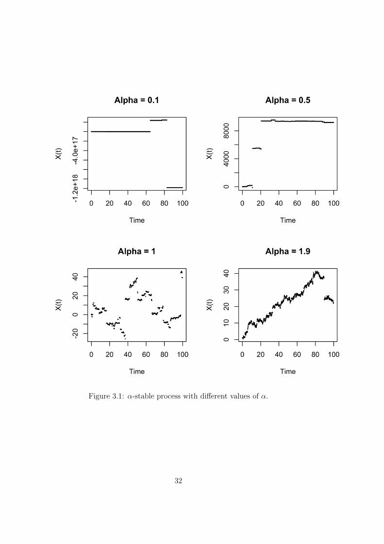
Figure 3.1: α-stable process with different values of α.

32

3.3 Derivative formula and gradients estimates

for SDE’s

On the topic of sensitivity analysis, there is a useful tool, or more precisely

a type of formula developed by Bismut-Elworty-Li. This has various ap-

plications in functional inequalities, heat kernels estimate and in our topic;

sensitivity analysis.

In the paper of Zhang [17] it’s proved a derivative formula of Bismut-

Elworthy-Li’s type for jump diffusion processes. He considers the interesting

α-stable process, where he along with the derivative formula derives a gra-

dient estimate for SDEs driven by α-stable noises, where α ∈ (0, 2). More

precisely the formula is for nonlinear SDEs, driven by an α-subordinated

Brownian motion (which is an α-stable process). In the literature, work re-

lated to this topic has been done by Cass and Fritz (see [17]), where they

proved a derivative formula of Bismut-Elworthy-Li’s type for SDE’s with

jumps. Also, Takeuchi (see [17]) worked out a formula for some pure-jump

diffusion, with finite moments of all orders. None of the works mentioned

above consider the α-stable process, which Zhang considers. Before we pro-

ceed to the results of Zhang, let’s recall some classical derivative formulas.

Let Btt≥0 be a standard d-dimensional Brownian motion. We are consid-

ering the following SDE in Rd:

dXt(x) = bt(Xt(x))dt+ σdBt, X0(x) = x, (3.9)

where σ is a d × d invertible matrix, and b : [0,∞)×Rd → Rd has continuous

first order partial derivatives with respect to x, and

||∇b||∞ < +∞,

here ∇bs(x) := (∂x1bs(x), ..., ∂xdbs(x)) and || · ||∞ denotes the uniform norm

with respect to s and x.

Furthermore there are two forms of derivative formulas: for f ∈ C1b (Rd)

and h ∈ Rd,

∇hEf(Xt(x)) =1

tE

(f(Xt(x))

∫ t

0

σ−1[h+ (t− s)∇hbs(Xs(x))]dBs

)(3.10)

and

∇hEf(Xt(x)) =1

tE

(f(Xt(x))

∫ t

0

σ−1∇hXs(x)dBs

), (3.11)

33

where for a function ϕ,∇hϕ := 〈∇ϕ, h〉 denotes the directional derivative

along h. In equation (3.11) ∇b needs to be bounded. ∇hXt(x) satisfies the

following linear equation:

∇hXt(x) = h+

∫ t

0

∇bs(Xs(x)) · ∇hXs(x)ds. (3.12)

Let α ∈ (0, 2) and let Stt≥0 be an independent α2-stable subordinator,

that is, an increasing R-valued process with stationary independent incre-

ments, and

E[eiuSt ] = et|u|α/2

, u ∈ R (i =√−1).

Letting St be defined in this way we have that the subordinated Brownian

motion BStt≥0 is an α-stable process.

Zhang’s formula assumes an SDE in Rd driven by BSt :

dXt(x) = bt(Xt(x))dt+ σ · dBSt , X0(x) = x.

Then we have the following theorem and what we refer to as Zhang’s formula,

that is, a formula for ∇Ef(Xt(x)):

Theorem 3.11. Under the condition that b : [0,∞)× Rd → Rd has contin-

uous first order partial derivatives with respect to x and ||∇b||∞ < +∞, for

any function f ∈ C1b (Rd) and h ∈ Rd, we have

∇hEf(Xt(x)) = E

(1

Stf(Xt(x))

∫ t

0

σ−1 · ∇hXs(x)dBSs

), (3.13)

where ∇hXs(x) is determined by equation (3.12). In particular, for any

α ∈ (0, 2) and p ∈ (1,∞], there exists a constant C = C(α, p) > 0 such that

for all t > 0,

|∇Ef(Xt(x))| ≤ C||σ−1||e||∇b||∞tt−1α (E|f(Xt(x))|p)

1p , (3.14)

where ||σ−1|| := sup|x|=1|σ−1x| and | · | denotes the Euclidean norm.

Remark. By equation (3.12) we see that s 7→ ∇hXs(x) is a bounded and

continuous σBSr : r ≤ s-adapted process. So the stochastic integral in

(3.13) makes sense.

Proof. See Theorem 1.1 in [17].

34

3.4 Simulation of the derivative of a caplet

with respect to the initial interest rate,

under the Vasicek interest rate model

In this section we will run simulations of eq. (3.13), with a stochastic interest

rate (Vasicek model), with the α-stable process, using high values of α, that is

α close to two. Then we will observe what the behavior is like when applying

the Brownian motion to Zhang’s formula, since we have the fact that an α

equal to two yields the Brownian motion.

3.4.1 The Vasicek interest rate model

The Vasicek model was introduced by Oldrich Vasicek in 1977, and was one

of the first interest rate models to capture mean reversion. Mean reversion is

the effect that either a high or a low interest rate will tend back to its average.

The average could for instance be determined by a country’s monetary policy.

In the real world a justification for using such a model, i.e. capture the mean

reversion effect, is because of too high interest rates will cause the economy

tend to slow down. A reason for this effect is that it becomes less profitable

to invest (e.g. borrow money from the bank). Hence an economy running

slowly would result in a lower interest rate. On the other hand, if the interest

rate is too low its not healthy for the economy, e.g. this could result in foreign

individuals from an arbitrary country, not demanding their currency because

it’s not profitable (to e.g. save money in banks). This will in turn result in

a bad currency rate, which is not healthy for the economy over time. Thus,

the interest rate would be driven up and tend to its average.

In the setting of Brownian motion the Vasicek model assumes that the

short rate evolves as an Ornstein-Uhlenbeck process, which is the solution of

an SDE on the form:

dXt = µXtdt+ σdBt.

More precisely the Vasicek short rate model is given by the following SDE:

drt = a(b− rt)dt+ σdBt, r(0) = r0, (3.15)

which has the solution (for proof see Lemma A.3.)

rt = r0e−at + b(1− e−at) + σe−at

∫ t

0

easdBs.

35

In the case of a jump diffusion we have that (Ls denotes a Levy process):

rt = x+

∫ t

0

a(b− rt)ds+

∫ t

0

σdLs, r0 = x (3.16)

The parameters r0, a, b and σ are non-negative, and can be interpreted as

follows:

r0 - Initial interest rate.

a - The speed at which the trajectories will go towards the mean (b) in

time.

b - Mean long term interest rate level.

σ - The volatility.

Dealing with Brownian motion we see that rt is normally distributed with

mean

E[rt] = r0e−at + b(1− e−at),

by using the fact that the expectation of an Ito integral is zero. Furthermore

rt has variance

V ar[rt] = V ar

[σe−at

∫ t

0

easdBs

]= σ2e−at

∫ t

0

(eas)2 ds

=σ2

2a(1− e−2at), (3.17)

where the second equality follows from the Ito isometry. If we look at the

average overnight interest rate, namely E[rt] and let t→∞ we see that

limt→∞

E[rt] = b and

E[rt] b if b ≥ r0

E[rt] b if b < r0.

One deficiency of the Vasicek model is that the interest rate rt, can become

negative, and the stochastic noise term does not depend on the evolution

of rt. On the other hand it is not a too complex model, in the sense that

36

it can be solved straight forward, in the setting of Brownian motion and

it is possible to estimate the parameters to historical data, by for instance

maximum likelihood estimation. One of the main reasons why we choose the

Vasicek model is because when we simulate equation (3.13) we have to use

a model satisfying equation (3.9), which demands that the volatility term

does not depend on the process itself. One might argue that this a limitation

of the forthcoming simulations, as one would expect that an interest rate

does not have constant volatility, but should depend on the interest rate

level. The Black-Karasinsky is a model which captures this effect, but cannot

be solved analytically as the Vasicek can. An alternative model could for

instance be the Cox Ingersoll Ross (CIR) model, which have advantages and

disadvantages compared to the Vasicek model. For more on this and other

interesting interest rate models see [2].

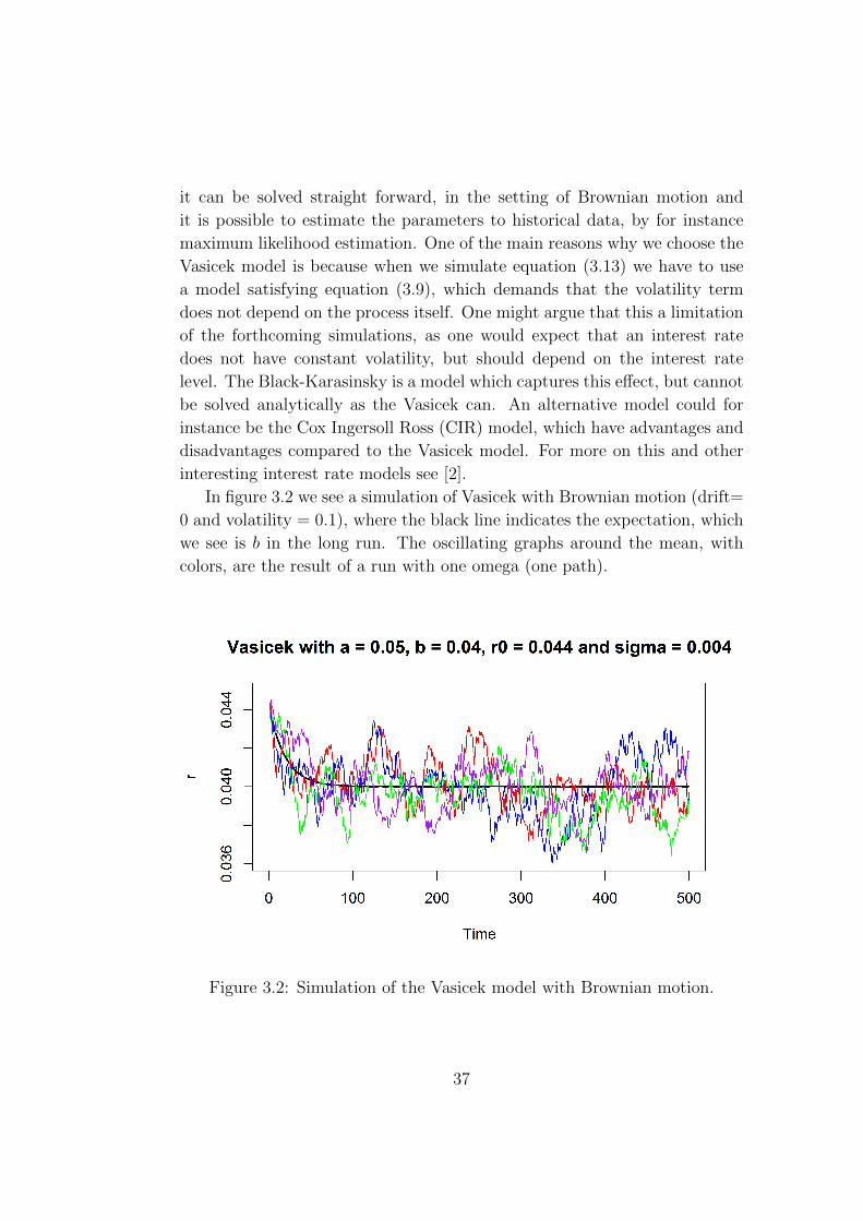
In figure 3.2 we see a simulation of Vasicek with Brownian motion (drift=

0 and volatility = 0.1), where the black line indicates the expectation, which

we see is b in the long run. The oscillating graphs around the mean, with

colors, are the result of a run with one omega (one path).

Figure 3.2: Simulation of the Vasicek model with Brownian motion.

37

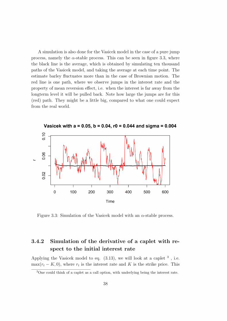
A simulation is also done for the Vasicek model in the case of a pure jump

process, namely the α-stable process. This can be seen in figure 3.3, where

the black line is the average, which is obtained by simulating ten thousand

paths of the Vasicek model, and taking the average at each time point. The

estimate barley fluctuates more than in the case of Brownian motion. The

red line is one path, where we observe jumps in the interest rate and the

property of mean reversion effect, i.e. when the interest is far away from the

longterm level it will be pulled back. Note how large the jumps are for this

(red) path. They might be a little big, compared to what one could expect

from the real world.

Figure 3.3: Simulation of the Vasicek model with an α-stable process.

3.4.2 Simulation of the derivative of a caplet with re-

spect to the initial interest rate

Applying the Vasicek model to eq. (3.13), we will look at a caplet 3 , i.e.

max(rt −K, 0), where rt is the interest rate and K is the strike price. This

3One could think of a caplet as a call option, with underlying being the interest rate.

38

could e.g. be the lowest interest rate an investor can handle. Thus he would

like to buy insurance to avoid a too low interest rate 4. Then we will take

the derivative of the caplet with respect to the initial interest r0 = x, and see

how this process evolves. The underlying process will be an α-stable process,

that is, the BSt-term will be an α-stable process. The Stt≥0-term denotes

the α2

subordinator. Applying eq. (3.13) we have the following:

f(Xt(x)) = max(rt −K, 0),

where rt is determined by the Vasicek interest rate model and K denotes the

strike price. Recall that in the scenario of jumps, the Vasicek model has the

following form:

rt = x+

∫ t

0

a(b− rs)ds+

∫ t

0

σdLs, (3.18)

where Ls is a Levy process. Taking the derivative of eq. (3.18) with respect

to the initial interest rate x, yields

d

dxrt = 1 +

∫ t

0

−a ddxrsds,

this a deterministic differential equation in which we get the solution ddxrt =

e−at, hence rt = xe−at. Arriving at σ, the d× d invertible matrix, we observe

that in our case that we have a 1× 1 matrix, thus the inverse σ−1 is just 1σ.

Inserting these ingredients into eq. (3.13) we get the following:

d

dxE[max(rt(x)−K, 0)] = E

[1

Stmax(rt(x)−K, 0)

∫ t

0

1

σ

d

dxrs(x)dBSs

]= E

[1

Stmax(rt(x)−K, 0)

∫ t

0

1

σ(1 +

∫ s

0

−a ddxru(x)du)dBSs

]= E

[1

Stmax(rt(x)−K, 0)

∫ t

0

1

σe−asdBSs

]. (3.19)

We will simulate eq.(3.19), using the Vasicek model where time goes from

0 to 600, in say days, where we observe a daily update on the interest rate,

meaning we use n = 600 uniformly distributed points in the Vasicek model.

For our underlying process, namely the α-stable process and α2-subordinator,

4If the investor can’t handle a high interest rate, then the investor can purchase the

opposite product, namely a floorlet.

39

we will choose a high α (meaning close to 2), say α = 1.999. Then we will

compare this to the case when α = 2, in which we are in the setting of the

Brownian motion. In the scenario α = 2 we let BSt = Bt, where Bt ∼ N(0, t)

is the Brownian motion, thus St becomes t under the expectation. Inserting

these ingredients into eq. (3.19) yields

d

dxE [max(rt(x)−K, 0)] = E

[1

tmax(rt(x)−K, 0)

∫ t

0

1

σe−asdBs

]. (3.20)

Simulating eq.(3.19) m = 1, 000, 000 times and obtaining the average by

the weighted average of each time point, we estimate

E(Xti) ≈1

m

m∑j=1

1

Stijmax(rti(x)−K, 0)

1

σ

∫ ti

0

e−asdBSsj.

Note that Sti and BSs are independent of each other for each j.

Implementing this in R, using a caplet on the interest rate, i.e.

max(rt − K, 0). Where the strike price is set to K = 0.05, r0 = 0.048,

long term interest rate b = 0.04, a = 0.05 (rate of which interest rate tends

towards b), the volatility σ = 0.004, which is used on both α = 1.999 and

α = 2, where we know the latter value for α means we are in the setting

of Brownian motion. When simulating the Brownian motion we arbitrary

choose drift = 0.06 and volatility = 0.5. These parameters could e.g. be

used by an investor who borrows money from a bank, to invest and needs

insurance in case of a high interest rate, here 5%, which might be due to

the costs related to paying interest on the loan the investor took out. The

investor knows the longterm interest rate is 0.04 (by the country’s monetary

policy), but also knows the rate fluctuates and hence wants protection. How

sensitive is this with respect to the initial interest rate?

40

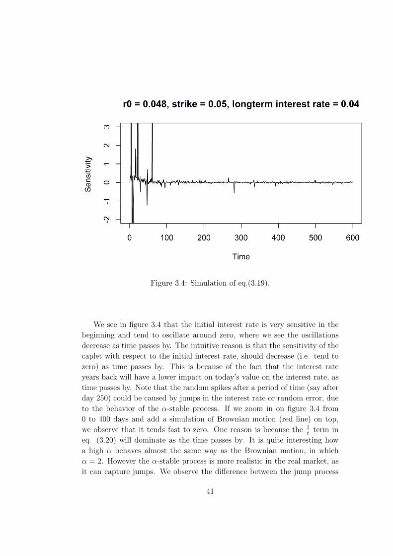
Figure 3.4: Simulation of eq.(3.19).

We see in figure 3.4 that the initial interest rate is very sensitive in the

beginning and tend to oscillate around zero, where we see the oscillations

decrease as time passes by. The intuitive reason is that the sensitivity of the

caplet with respect to the initial interest rate, should decrease (i.e. tend to

zero) as time passes by. This is because of the fact that the interest rate

years back will have a lower impact on today’s value on the interest rate, as

time passes by. Note that the random spikes after a period of time (say after

day 250) could be caused by jumps in the interest rate or random error, due

to the behavior of the α-stable process. If we zoom in on figure 3.4 from

0 to 400 days and add a simulation of Brownian motion (red line) on top,

we observe that it tends fast to zero. One reason is because the 1t

term in

eq. (3.20) will dominate as the time passes by. It is quite interesting how

a high α behaves almost the same way as the Brownian motion, in which

α = 2. However the α-stable process is more realistic in the real market, as

it can capture jumps. We observe the difference between the jump process

41

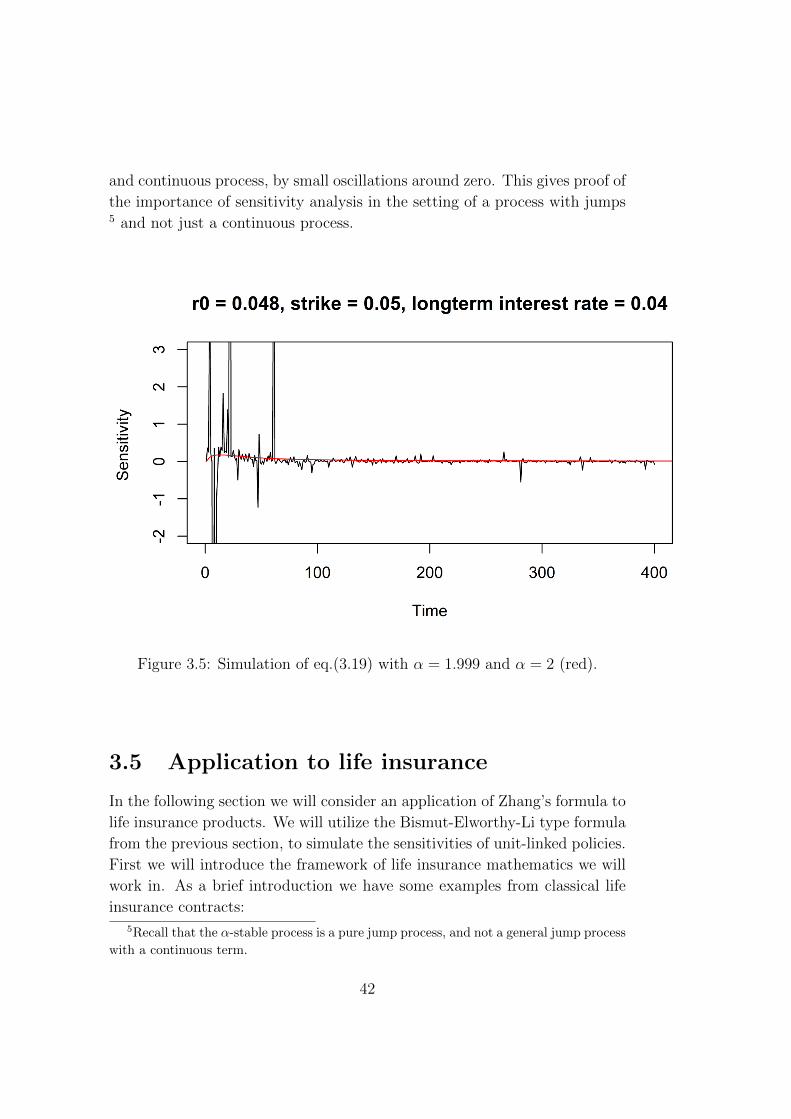
and continuous process, by small oscillations around zero. This gives proof of

the importance of sensitivity analysis in the setting of a process with jumps5 and not just a continuous process.

Figure 3.5: Simulation of eq.(3.19) with α = 1.999 and α = 2 (red).

3.5 Application to life insurance

In the following section we will consider an application of Zhang’s formula to

life insurance products. We will utilize the Bismut-Elworthy-Li type formula

from the previous section, to simulate the sensitivities of unit-linked policies.

First we will introduce the framework of life insurance mathematics we will

work in. As a brief introduction we have some examples from classical life

insurance contracts:

5Recall that the α-stable process is a pure jump process, and not a general jump process

with a continuous term.

42

Pure endowment: Payment from the insurer to the insured, when

the insured reaches ages of maturity of the policy. In case of death

before reaching the time of maturity of the policy, there is no payment.

Term-life insurance: If the individual dies before the age of maturity

of the policy, the heirs receive a payment.

Endowment: Sum of a pure endowment insurance and a term life

insurance. Which means that the individual holding such a contract

will receive a payment (to the heirs), in case of an early death. If the

individual reaches the time of maturity of the policy, then the individual

receives payment.

The following presentation of the framework in life insurance, is based on

chapter 2 in [11]. In the following section we will present an application to

life-insurance products, more precisely unit linked policies.

3.5.1 Framework in life insurance

To be able to deal with life insurance we need some basic knowledge of

transition probabilities between states, e.g. probability of going from the

state alive to dead or alive to disabled. For our purposes we will only need

the state alive or dead, denoted respectively by (*, ). To obtain the transition

probabilities we will resort to Kolmogorov’s differential equations, where we

first need the knowledge of what transition rates are, and what a regular

Markov chain is.

Definition 3.12. Let (Xt)t∈T be a Markov chain with finite state space S

and T ⊂ R. For N ⊂ S we define

pjN(s, t) :=∑k∈N

pjk(s, t).

Definition 3.13. (Transition rates) Let X(t)t∈T be a Markov chain in con-

tinuous time with finite state space S. (Xt)t∈T is called regular, if

µi(t) = lim∆t0

1− pii(t, t+ ∆t)

∆tfor all i ∈ S (3.21)

µij(t) = lim∆t0

pij(t, t+ ∆t)

∆tfor all i 6= j ∈ S (3.22)

are well defined and continuous with respect to t.

43

The functions µi(t) and µij are called transition rates. Also

µii(t)def= −µi(t), i ∈ S.

Remark. The transition rates can be interpreted as derivatives of the

transition probabilities. For i 6= j we get

µij(t) = lim∆t0

pij(t, t+ ∆t)

∆t

= lim∆t0

pij(t, t+ ∆t)− pij(t, t)∆t

=d

dspij(t, s)|s=t.

µijdt can be interpreted as the infinitesimal transition rate from i to j

in the time interval [t, t+ dt]. Furthermore Λ(t) is defined as

Λ(t) =

µ11(t) µ12(t) µ13(t) . . . µ1n(t)

µ21(t) µ22(t) µ23(t) . . . µ2n(t)...

......

. . ....

µn1(t) µn2(t) µn3(t) . . . µnn(t)

where Λ generates the behavior of a Markov chain. Hence we have that

Λ = lim∆t→0

P (∆t)− 1

∆t.

Λ := Λ(0) is called the generator of the one parameter semigroup. P (t)

can be reconstructed by

P (t) = exp(tΛ) =∞∑n=0

tn

n!Λn

How do we obtain the transition probabilities from one state to another?

Given a state space, consisting of different states e.g. alive, ill, critically ill

and dead, how does one find the probabilities? The answer, is to solve the

Kolmogorov differential equations:

Theorem 3.14. (Kolmogorov) Let (Xt)t∈T be a regular Markov chain on a

finite state space S. Then the following statements hold:

44

1. (Backward differential equations)

d

dspij(s, t) = µi(s)pij(s, t)−

∑k 6=i

µik(s)pkj(s, t), (3.23)

d

dsP (s, t) = −Λ(s)P (s, t) (3.24)

2. (Forward differential equations)

d

dtpij(s, t) = −pij(s, t)µj(t) +

∑k 6=j

pik(s, t)µkj(t), (3.25)

d

dtP (s, t) = P (s, t)Λ(t). (3.26)

Proof. See proof of Theorem 2.3.4 in [11].

As mentioned earlier, we will need the transition probabilities for a model

concerning the two states alive and dead (*, ). The simplest transition rate

of µ∗† would be to set it equal to a constant. This is not very realistic, as one

can imagine, there is a higher probability of not dying given that the person

is young (say 20 years old), than an old person (say 80 years old). We will

use a death rate estimated from [11]. More precisely a polynomial of degree

two was fitted to log(µ∗†):

µ∗† = exp(−7.85785 + 0.01538 · x+ 5.77355 · 10−4 · x2) (3.27)

Using the fact that

µi(t) =∑j 6=i

µij(t)

and the Kolmogorov forward differential equations (eq. 3.25) we get

d

dtp∗∗(s, t) = −p∗∗(s, t)µ∗(t) + p∗†(s, t)µ†∗(t) (3.28)

d

dtp∗†(s, t) = −p∗†(s, t)µ†(t) + p∗∗(s, t)µ∗†(t), (3.29)

where we note that µ† = 0 and µ†∗ = 0. Solving eq. (3.28) yields

45

d

dtp∗∗(s, t) = −p∗∗(s, t)µ∗†(t)

ddtp∗∗(s, t)

p∗∗(s, t)= −µ∗†(t)

d

dtln(p∗∗(s, t)) = −µ∗†(t)

p∗∗(s, t) = exp(−∫ t

s

µ∗†(u)du). (3.30)

As for eq. (3.29) we note that since there are two states, namely dead

and alive that we only have the transition probabilities p∗∗(s, t) and p∗†(s, t)

(And of course the trivial states p††(s, t) = 1 and p†∗(s, t) = 0). Thus the

solution for p∗†(s, t) becomes

p∗†(s, t) = 1− exp(−∫ t

s

µ∗†(u)du) (3.31)

3.5.2 Unit-linked policies

In the world of life insurance there are numerous contracts and policies, e.g.

a lump sum payment in case of death, disability payments if one becomes

ill, pension schemes etc. Unit-linked policies are insurance contracts where

the policyholder gets the benefit of both investment and insurance. The

investments could for instance be in stocks or bonds. This type of policy

usually has a single premium. We will look at two unit-linked policies, namely

an endowment policy, which is represented in the following way:

V (0) = EQ[exp(−δT )C(T )] · TPs. (3.32)

Here we have that

TPs = p∗∗(s, s+ 1) · p∗∗(s+ 1, s+ 2) · · · p∗∗(s+ T − 1, s+ T )

denotes the probability of surviving over the period of the contract, when the

individual is s years old at the beginning of the contract, and T is number

of periods (years) ahead.

Furthermore we have a term life insurance:

V (0) =

∫ T

0

EQ[exp(−δt)C(t)]p∗∗(s, s+ t)µ∗†(s+ t)dt. (3.33)

46

Here V (0) denotes the single premium. The expectation is taken with

respect to the risk neutral measure Q, exp(−δt) is the discount factor where

δ is a constant. C(t) is the payoff function (where C(t) is stochastic), which

could e.g. be max(rt − K, 0) (caplet) where rt is a stochastic interest rate

and K is the strike price. C(t) could also e.g. be a guaranteed return,

i.e. max(N(t)S(t), G(t)) where N(t) is the number of shares bought of an

arbitrary stock. Where S(t) denotes the stochastic stock price function, e.g.

S(t) = xeLt for a Levy process Lt, the initial value x of the stock and G(t)

the guarantee are set equal to a fixed number.

One might be interested in what V (t) is in general, not just V (0). If

we assume we have a filtration Ft of information up to time t, which is a

σ-algebra, then we can have a look at the sensitivity of V (t). Let us consider

the sensitivity of an endowment policy with respect to an x, where x is a

parameter of the stochastic payout function C(t). Using the Markov property

of rt (we assume that rt is the risk neutral process), we have the following

for V (t), at a future time point t.

d

dxV (t) =

d

dxEQ[e−δTmax(rT −K, 0)|Ft] · TPs

= e−δTd

dyEQ[max(ry,tT−t −K, 0)]|y=rxt

· ddxrxt · TPs (3.34)

Similar computations for the term life insurance, with say a put option

with strike price K (makes the payoff function C(t) bounded). Where the

number of shares bought are noted by N(t) and the guarantee is noted by

G(t). Assuming both of the latter functions are constants, we obtain:

d

dxV (t) =

d

dx

∫ T

t

EQ[e−δumax(K −N(u)S(u), G(u))|Ft] · p∗∗(s, s+ u)µ∗†(s+ u)du

=

∫ T

t

e−δud

dxEQ[max(K −N(u)S(u), G(u))|Ft] · p∗∗(s, s+ u)µ∗†(s+ u)du

=

∫ T

t

e−δud

dyEQ[max(K −N(u)Sy,t(u− t), G(u)]|y=S(t)

· ddySy(t) · p∗∗(s, s+ u)µ∗†(s+ u)du (3.35)

Where S(t) could e.g. be an exponential Levy process, i.e.

S(t) = xeσLt , where x = S(0),

47

so

d

dxS(t) =

d

dxxeσLt

= eσLt . (3.36)

Using eq. (3.36) in connection with the sensitivity of the term life insur-

ance (eq. (3.35)) we obtain

d

dxV (t) =

∫ T

t

e−δud

dyEQ[max(K −N(u)S(u− t), G(u))]|y=S(t)

d

dyS(t) · p∗∗(s, s+ u)µ∗†(s+ u)du

=

∫ T

t

e−δud

dxEQ[max(K −N(u)yeσLu−t , G(u))]|y=S(t) · eσLt·

p∗∗(s, s+ u)µ∗†(s+ u)du (3.37)

Furthermore in both eq. (3.34) and eq. (3.37) we can apply Zhang’s

formula, namely eq. (3.13) for the derivative of the expectation to obtain a

solution.

3.5.3 Simulation of the sensitivity of unit-linked poli-

cies

Let’s have a look at eq. (3.34) at t = 0 (beginning of the contract) in

connection with a caplet, i.e. let C(t) = max(rt − K, 0) where we let the

interest rate process rt be modeled by the Vasicek model with jumps (see eq.

(3.18)). The parameters for the Vasicek model are chosen to be

r0 = 0.048 (Initial interest rate).

a = 0.05 (Rate of convergence to the longterm interest rate).

b = 0.04 (Longterm interest rate).

σ = 0.004 (Volatility).

48

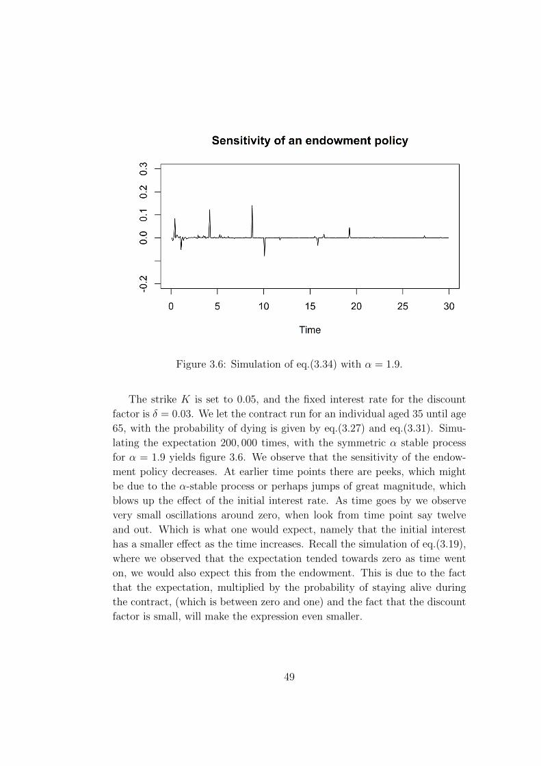
Figure 3.6: Simulation of eq.(3.34) with α = 1.9.

The strike K is set to 0.05, and the fixed interest rate for the discount

factor is δ = 0.03. We let the contract run for an individual aged 35 until age

65, with the probability of dying is given by eq.(3.27) and eq.(3.31). Simu-

lating the expectation 200, 000 times, with the symmetric α stable process

for α = 1.9 yields figure 3.6. We observe that the sensitivity of the endow-

ment policy decreases. At earlier time points there are peeks, which might

be due to the α-stable process or perhaps jumps of great magnitude, which

blows up the effect of the initial interest rate. As time goes by we observe

very small oscillations around zero, when look from time point say twelve

and out. Which is what one would expect, namely that the initial interest

has a smaller effect as the time increases. Recall the simulation of eq.(3.19),

where we observed that the expectation tended towards zero as time went

on, we would also expect this from the endowment. This is due to the fact

that the expectation, multiplied by the probability of staying alive during

the contract, (which is between zero and one) and the fact that the discount

factor is small, will make the expression even smaller.

49

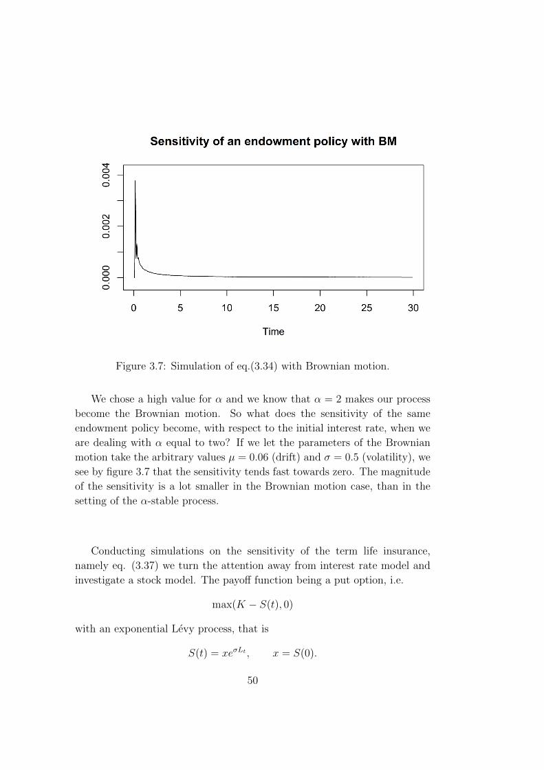
Figure 3.7: Simulation of eq.(3.34) with Brownian motion.

We chose a high value for α and we know that α = 2 makes our process

become the Brownian motion. So what does the sensitivity of the same

endowment policy become, with respect to the initial interest rate, when we

are dealing with α equal to two? If we let the parameters of the Brownian

motion take the arbitrary values µ = 0.06 (drift) and σ = 0.5 (volatility), we

see by figure 3.7 that the sensitivity tends fast towards zero. The magnitude

of the sensitivity is a lot smaller in the Brownian motion case, than in the

setting of the α-stable process.

Conducting simulations on the sensitivity of the term life insurance,

namely eq. (3.37) we turn the attention away from interest rate model and

investigate a stock model. The payoff function being a put option, i.e.

max(K − S(t), 0)

with an exponential Levy process, that is

S(t) = xeσLt , x = S(0).

50

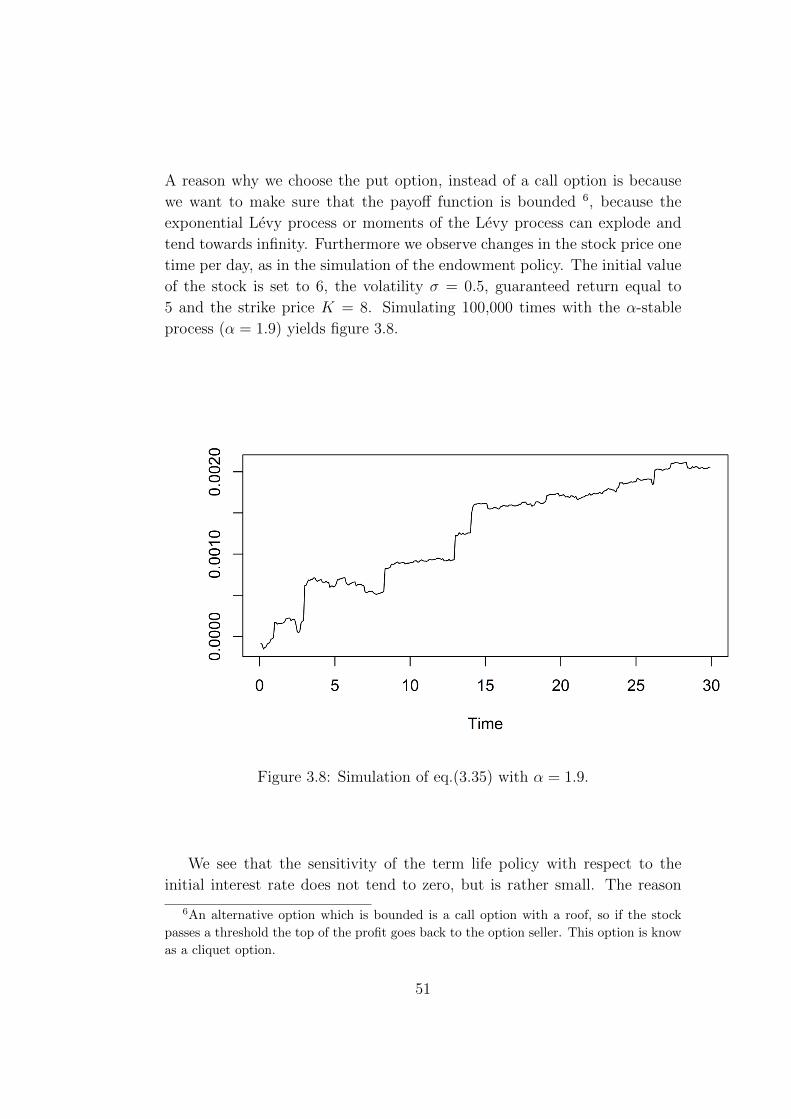
A reason why we choose the put option, instead of a call option is because

we want to make sure that the payoff function is bounded 6, because the

exponential Levy process or moments of the Levy process can explode and

tend towards infinity. Furthermore we observe changes in the stock price one

time per day, as in the simulation of the endowment policy. The initial value

of the stock is set to 6, the volatility σ = 0.5, guaranteed return equal to

5 and the strike price K = 8. Simulating 100,000 times with the α-stable

process (α = 1.9) yields figure 3.8.

Figure 3.8: Simulation of eq.(3.35) with α = 1.9.

We see that the sensitivity of the term life policy with respect to the

initial interest rate does not tend to zero, but is rather small. The reason

6An alternative option which is bounded is a call option with a roof, so if the stock

passes a threshold the top of the profit goes back to the option seller. This option is know

as a cliquet option.

51

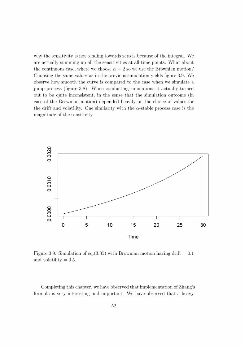
why the sensitivity is not tending towards zero is because of the integral. We

are actually summing up all the sensitivities at all time points. What about

the continuous case, where we choose α = 2 so we use the Brownian motion?

Choosing the same values as in the previous simulation yields figure 3.9. We

observe how smooth the curve is compared to the case when we simulate a

jump process (figure 3.8). When conducting simulations it actually turned

out to be quite inconsistent, in the sense that the simulation outcome (in

case of the Brownian motion) depended heavily on the choice of values for

the drift and volatility. One similarity with the α-stable process case is the

magnitude of the sensitivity.

Figure 3.9: Simulation of eq.(3.35) with Brownian motion having drift = 0.1

and volatility = 0.5.

Completing this chapter, we have observed that implementation of Zhang’s

formula is very interesting and important. We have observed that a heavy

52

theoretical formula used for computation in sensitivity analysis, yields the

results one would expect. We observed how the sensitivity of a caplet, with

respect to the initial interest rate tended towards zero. This also became evi-

dent as we ran more simulations in the section of application to life insurance

using Zhang’s formula.

We do however note some limitations in Zhang’s formula. The coefficients

b in the dynamics (3.9) is assumed to have continuous first order derivative.

A class with worse 7 coefficients we will investigate in the next chapter are

Holder coefficients. Here we show a Bismut-Elworthy-Li type formula, in the

case of the Greek Delta.

7In the sense that we do not have as nice properties as a coefficient b ∈ C1(R), which

is bounded.

53

54

Chapter 4

Derivation of the delta in the

case of SDE’s with Holder drift

coefficients

In this chapter we will derive a ”derivative free” representation for the Greek

delta (i.e. we will derive a Bismut-Elworthy-Li type formula). This is a new

formula which is of the form (3.13), but has the new feature that we will be

able to deal with a larger class of coefficients b. The derivation of the formula

uses results from [8], as they derive results concerning SDE’s on the same

form we will work with, that is, with Holder coefficients. We will use this

paper in connection with [17].

The following chapter is divided into three sections, where the first section

introduces the framework and states ”computational rules” needed further

on. Also we include a short summary of the paper [8]. In section two we

state two lemmas, with proofs, which are needed for the main theorem of

this chapter. The first lemma ensures uniform boundedness of derivatives of

a approximating stochastic flows in the L2 we will work with. Then, in the

second lemma, we show that the SDE-solution with Holder drift coefficient

in the forthcoming Bismut-Elworthy-Li formula, is Soboblev differentiable.

The important Bismut-Elworthy-Li formula for the Greek Delta with Holder

coefficients is given in a theorem, presented in the last section of this chapter.

55

4.1 Framework

The main paper used, to be able to derive the forthcoming lemmas and final

theorem is the paper [8], where they use a new method to construct unique

strong solutions of SDE’s with singular coefficients. Let’s consider an SDE

of the form

Xt = x+

∫ t

0

b(s,Xs)ds+ Lt, 0 ≤ t ≤ T, x ∈ Rd (4.1)

where b : [0, T ]×R −→ Rd is a Borel-measurable function and Lt, 0 ≤ t ≤ T is

a d-dimensional (square integrable) Levy process. So the process is on some

complete probability space (Ω,F , µ), that has stationary and independent

increments starting at zero. In fact, we have that b is singular in the sense

that b is bounded and β - Holder continuous, i.e.

||b||Cβb := sup0≤t≤T,x∈Rd

|b(t, x)|+ sup0≤t≤T

supx 6=y

|b(t, x)− b(t, y)||x− y|β

<∞,

where 0 < β < 1. We know (by Picard iteration) that if b is Lipschitz

continuous that there exists a unique strong solution Xt, 0 ≤ t ≤ T to (4.1).

This type of solution is used in a variety of applications, such as in statistical

mechanics or in the theory of controlled diffusion processes. In the literature

there are results when b is singular and Lt is a Wiener process. On the other

hand, we have the case when Lt is a pure jump Levy process. The aim of [8]

is to introduce a new technique to construct unique strong solutions to (4.1).

The way this is done, is by approximating the singular coefficients b in (4.1)

by smooth functions bn. So

Xnt = x+

∫ t

0

bn(s,Xns )ds+ Lt, 0 ≤ t ≤ T, x ∈ Rd

for each n ≥ 1. Then the authors apply a compactness criterion based on

Malliavin calculus in connection with PDE-techniques to the sequence of

solutions Xnt , n ≥ 1 to obtain a unique strong solution Xt. One important

feature of this technique is that the solutionXt will be Malliavin differentiable

for all t.

Framework

We now proceed to introduce the framework we are working in, for the

remainder of this chapter.

Martingale is in the ordinary sense, i.e.:

56

Definition 4.1. A filtration (on (Ω,F )) is a family M = Mtt≥0 of σ-

algebras Mt ⊂ F such that

0 ≤ s < t⇒Ms ⊂Mt.

An n-dimensional stochastic process Mtt on (Ω,F , P ) is called a martin-

gale with respect to a filtration Mt≥0 if

i) Mt is Mt-measurable for all t,

ii) E[|Mt|] <∞ for all t

iii) E[Ms|Mt] = Mt for all s ≥ t.

We need the Ito isometry in the case of Levy processes:

Let X(t) ∈ Rn be an Ito - Levy process of the form

dX(t) = α(t, ω)dt+ σ(t, ω)dB(t) +

∫Rlγ(t, z, ω)N(dt, dz). (4.2)

where α : [0, T ]×Ω→ Rn, σ : [0, T ]×Ω→ Rn×m, and γ : [0, T ]×Rl×Ω→ Rd

are adapted processes such that the integrals exist. Here B(t) is an m-

dimensional Brownian motion. Also,

N(dt, dz) =

N(dt, dz)− ν(dz)dt if |z| < R

N(dt, dz) if |z| ≥ R

for some R ∈ [0,∞].

Theorem 4.2 (The Ito-Levy isometry). Let X(t) ∈ Rd be as in (4.2) but

with X(0) = 0 and α = 0. Then

E[X2(T )] = E

[∫ T

0

(n∑i=1

m∑j=1

σ2ij(t) +

n∑i=1

l∑j=1

∫Rγ2ij(t, zj)νj(dzj)

)dt

]

=n∑i=1

E

[∫ T

0

(m∑j=1

σ2ij(t) +

l∑j=1

∫Rγ2ij(t, zj)νj(dzj)

)dt

](4.3)

provided that the right-hand side is finite.

57

Proof. Theorem 1.17 in [19].

Remark. As a special case of Theorem 4.2 assume that

dX(t) = dη(t) =

∫RzN(dt, dz) ∈ R

with E[X2(T )] = T∫R z

2ν(dz) <∞. Then we have the isometry

E

[(∫ T

0

H(t)dη(t)

)2]

= E

[∫ T

0

H2(t)dt

] ∫Rz2ν(dz) (4.4)

for all H ∈ Lucp such that H ∈ L2([0, T × Ω]), i.e., such that

||H||L2([0,T ]×Ω) := E

[∫ T

0

H2(T )dt

]<∞.

Lucp denotes the space of adapted caglad processes (left continuous with right

limits), for more on this consult [19].

Gronwall inequality

We will use an inequality called the Gronwall inequality 1.

This inequality states that if we have a non-negative function v(t) such

that

v(t) ≤ C + A

∫ t

0

v(s)ds, for 0 ≤ t ≤ T

for constants C,A where A ≥ 0 then

v(t) ≤ C · exp(At), for 0 ≤ t ≤ T.

Furthermore we will encounter the Sobolev space W 1,2loc which consists

of the subset of functions f ∈ L2(R), such that the derivative up to order

1 exists in the weak sense and belongs to L2. More precisely we have the

following definition:

Definition 4.3. For a u ∈ W 1,2loc (Rd)⇔ ∀y ∈ Rd ∃U open, bounded subset

with y ∈ U such that u ∈ W 1,2(U). Where the space W 1,2 is defined as

W 1,2 def= u ∈ L2(u) :

∫U

u(x)∂

∂xiφ(x)dx = −

∫U

f(x)φ(x)dx

1If one is interested in how to show that the inequality holds see exercise 5.17 in [18].

58

for all φ ∈ C∞c (U) for some f ∈ L2(U),

where C∞c denotes the space of functions that has compact support and all

orders of the derivatives are continuous.

In the proof we will use the Ito formula 2, that is presented in Ikeda and

Watanabe, namely Theorem 5.1 in [9]. This is due to the form of the SDE-

solution we will work with, where the stochastic part of the SDE-solution is

of the form

Lt =

∫ t+

0

∫Rdz · 1||z||>1N(ds, dz)

+

∫ t+

0

∫Rdz · 1||z||≤1N(ds, dz).

Using the Ito formula presented in chapter 3 in this setting is rather cum-

bersome, compared to the Ito formula presented in Ikeda and Watanabe.

Furthermore, for β ∈ (0, 1) and k, d ≥ 1 the space Cβb (Rd,R) will denote a

space of continuous functions u : Rd → R, which we will use on the simplified

form Cβb (Rd) = Cβ

b (Rd,R). This space is also known as the space of bounded

β - Holder continuous functions, which is equipped with the norm

||u||Cβb (Rd) = ||u||∞ + supx 6=y|u(x)− u(y)||x− y|β

<∞,

where ||u||∞ := supx∈Rd |u(x)|.Also, C∞(Rd) denotes the space of bounded continuous functions van-

ishing at infinity, with respect to the supremum norm || · ||∞. So C2∞(Rd)

denotes the space of all f ∈ C2b (Rd) ∩ C∞(Rd), so that its first and second

order partial derivative belong to C∞(Rd).

In the following sections we will encounter weak convergence 3:

Definition 4.4. Weak convergence in L2(Ω):

Xn X in L2(Ω)

⇔E[Y Xn] −−−→

n→∞E[Y ·X] for all Y ∈ L2(Ω).

2Note that we work with the Ito-Levy formula, not the classic Ito formula with the

Brownian motion.3We will later on work with a sequence where we let Xn

def= ∂

∂xXx,nt .

59

The proof of Lemma 4.6 is based on Kolmogrov’s equation, thus we need

the following theorem:

Theorem 4.5. Let Lt, 0 ≤ t ≤ T be a d-dimensional α-stable process for

α ∈ (1, 2). Require that φ ∈ C([0, T ], Cβb (Rd)) for β ∈ (0, 1) with α + β > 2.

Then there exist a u ∈ C([0, T ], C2b (Rd)) ∩ C1([0, T ], Cb(Rd)) satisfying the

backward Kolmogorov equation

∂

∂tu+ b · ∇u+ L u = −φ on [0, T ], u |t=T= 0. (4.5)

Moreover

||Du||Cβb ≤ C(T )||φ||Cβb (4.6)

where

C(T )→ 0 for T 0,

as well as

||D2u||∞ ≤M · ||φ||Cβb (4.7)

for a constant M.

Proof. Theorem 17 in [8].

Remark.

(L f)(x) =

∫Rdf(x+ y)− f(x)− y · 1||y||≤1 ·Df(x)ν(dy),

where ν denotes the Levy measure and f ∈ C2∞(Rd).

4.2 Properties of an SDE with Holder coeffi-

cients

In this section we state and show two Lemmas, needed to be able to prove

the theorem in the next section.

60

Lemma 4.6. Let

Xx,nt = x+

∫ t

0

bn(Xx,ns )ds+ Lt,

where Lt, 0 ≤ t ≤ T is a d-dimensional α-stable process, where α ∈ (1, 2)

and bn ∈ C([0, T ];C∞c (Rd)), where β ∈ (0, 1) such that ||bn||Cβb ≤ ||b||Cβb for

all n. Furthermore require that α + β > 2 and α > 2β then

supx∈Rd,n≥1

E

[|| ∂∂xXx,nt ||2

]<∞.

Proof. Consider now the SDE-solutions

Xx,nt = x+

∫ t

0

bn(Xx,ns )ds+ Lt, 0 ≤ t ≤ T, n ≥ 0, (4.8)

where

Lt =

∫ t+

0

∫Rdz · 1||z||>1N(ds, dz)

+

∫ t+

0

∫Rdz · 1||z||≤1N(ds, dz) (4.9)

is an α-stable process such that α + β > 2 for α ∈ (1, 2) and β ∈ (0, 1) and

where bn ∈ C([0, T ];C∞c (Rd)), n ≥ 1 such that

||bn||Cβb ≤ ||b||Cβb

for all n and

bnk(·) −→ b(·) in Cδ(K)

for all t, any compact set K ⊂ Rd and 0 < δ < β for a subsequence nk,

k ≥ 1 depending on K. Using Theorem 4.5 in connection with Ito’s lemma

61

4 applied to Xx,nt , 0 ≤ t ≤ T , n ≥ 1 we get 5

u(t,Xx,nt ) = u(0, x) +

∫ t

0

∂

∂su(s,Xx,n

s )ds

+

∫ t

0

∂

∂xu(s,Xx,n

s ) · b(Xx,ns )ds

+

∫ t+

0

∫Rdu(s,Xx,n

s− + γ1(z))− u(s,Xx,ns− )N(ds, dz)

+

∫ t+

0

∫Rdu(s,Xx,n

s− + γ2(z))− u(s,Xx,ns− )N(ds, dz)

+

∫ t

0

∫Rdu(s,Xx,n

s + γ2(z))− u(s,Xx,ns )− γ2(z) ·Dxu(s,Xx,n

s )ν(dz)ds

= u(0, x) +

∫ t

0

b(Xx,ns )ds

+

∫ t+

0

∫Rdu(s,Xx,n

s− + γ1(z))− u(s,Xx,ns− )N(ds, dz)

+

∫ t+

0

∫Rdu(s,Xx,n

s− + γ2(z))− u(s,Xx,ns− )N(ds, dz),

where

γ1(z) := 1||z||>1 · z and γ2(z) := 1||z||≤1 · z

on Rd.

So we obtain that

Xx,nt = x+ u(t,Xx,n

t )− u(0, x)

−∫ t+

0

∫Rdu(s,Xx,n

s− + γ1(z))− u(s,Xx,ns− )N(ds, dz)

−∫ t+

0

∫Rdu(s,Xx,n

s− + γ2(z))− u(s,Xx,ns− )N(ds, dz)

+ Lt (4.10)

We know from [14] that

x 7−→ Xx,nt

4The version of Ito’s lemma used is the one on page 66 in [9].5Where the function u is the solution to the backward Kolmogorov equation in theorem

4.5

62

is continuously differentiable for all t, n with probability 1. So taking the

partial derivative with respect to x and using the mean value theorem 6 we

get that

∂

∂xXx,nt = Id+Du(t,Xx,n

t )∂

∂xXx,nt −Du(0, x)

−∫ t+

0

∫Rd

(Du(s,Xx,ns− + γ1(z))−Du(s,Xx,n

s− ))∂

∂xXx,ns− N(ds, dz)

−∫ t+

0

∫Rd

(∫ 1

0

D2u(s,Xx,ns− + θγ2(z))

∂

∂xXx,ns− dθ · γ2(z)

)N(ds, dz),

(4.11)

where Id denotes the identity matrix. Let α > 2β in addition. Then it

follows from Theorem 4.5 in connection with the Ito-Levy isometry that

E

[|| ∂∂xXx,nt ||2

]≤ K1 + E

[||Du(t,Xx,n

t )∂

∂xXx,nt ||2

]+ E

[||∫ t+

0

∫Rd

((Du(s,Xx,n

s− + γ1(z))−Du(s,Xx,ns− ))

∂

∂xXx,ns−

)N(ds, dz)||2

]+ E

[||∫ t+

0

∫Rd

(∫ 1

0

D2u(s,Xx,ns− + θγ2(z))

∂

∂xXx,ns− dθγ2(z)

)N(ds, dz)||2

]

≤ K1 + (C(T ))2||bn||2Cβb E[|| ∂∂xXx,nt ||2

]+

∫ t

0

E

[|| ∂∂xXx,ns ||2

]ds

∫Rd||Du(s,Xx,n

s− + γ1(z))−Du(s,Xx,ns− )||2ν(dz)

+

∫ t

0

E

[|| ∂∂xXx,ns ||2

]ds

∫Rd

∫ 1

0

||D2u(s,Xx,ns− + θγ2(z))||2dθ||γ2(z)||2ν(dz)

6We will use an integral form of the mean value theorem (this form of the mean value

theorem is known as Hadamard’s mean value theorem), which is of the form f(x + h) −f(x) =

∫ 1

0f ′(x+ θ · h)dθ · h. Where we let h = γ1(z) in the proof.

63

≤ K1 + (C(T ))2||bn||2Cβb E[|| ∂∂xXx,nt ||2

]+

∫ t

0

E

[|| ∂∂xXx,ns ||2

]ds

∫Rd

||Du(s,Xx,ns− + γ1(z))−Du(s,Xx,n

s− )||2

||γ1(z)||2β

· ||γ1(z)||2βν(dz)

+

∫ t

0

E

[|| ∂∂xXx,ns ||2

]ds

∫Rd

∫ 1

0

M2||bn||2Cβb dθ||γ2(z)||2ν(dz)

≤ K11 + (C(T ))2 · ||bn||2Cβb · E[|| ∂∂xXx,nt ||2

]+ (C(T ))2||bn||2Cβb

∫Rd||γ1(z)||2βν(dz)

∫ t

0

E

[|| ∂∂xXx,ns ||2

]ds

+M2||bn||2Cβb ·∫Rd||γ2(z)||2ν(dz)

∫ t

0

E

[|| ∂∂xXx,ns ||2

]ds,

where K1 is a constant, and

E

[∫ t

0

|| ∂∂xXx,ns− ||

2ds

]= E

[∫ t

0

|| ∂∂xXx,ns ||2ds

].

So we get that

E[|| ∂∂xXx,nt ||2] ≤ 1

1−K1(C(T ))2||bn||2Cβb

·K1(1 + C

∫ t

0

E[|| ∂∂xXx,ns ||2]ds)

Thus Gronwall’s Lemma gives

E[|| ∂∂xXx,nt ||2] ≤ K1

1−K1(C(T ))2||bn||2Cβb

· exp

(T · C ·K1

1−K1(C(T ))2||bn||2Cβb

),

where we choose T such that

1−K1(C(T ))2||bn||2Cβb ≥1

2

64

uniformly in n. Hence we obtain that

supx∈Rd,n≥1

E[|| ∂∂xXx,nt ||2] <∞.

In the sequel we aim at using Lemma 4.6 to prove that Xxt satisfying

Xxt = x+

∫ t

0

b(Xxs )ds+ Lt 0 ≤ s ≤ T

is Sobolev differentiable in x ∈ Rd for all t and almost all ω, if b is Holder

continuous.

Lemma 4.7. Assume that α + β > 2, α > 2β for some α ∈ (1, 2) and

β ∈ (0, 1). Furthermore, suppose that b ∈ Cβb (Rd). Then the solution Xx

t ,

0 ≤ t ≤ T associated with b is Sobolev differentiable, that is

(x −→ Xxt (ω)) ∈ W 1,2

loc (Rd)

for all t and ω ∈ Ω with P (Ω) = 1

Proof. Consider the approximating sequence bn of coefficients to b in Lemma

4.6. It is known in this case that

X.x,n −−−→n→∞

X.x in L2([0, T ]× Ω) (4.12)

(at least for a subsequence) see [16]. Choose now φ ∈ C∞c (U) for a bounded

open set U ⊆ Rd and τ ∈ L∞([0, T ]× Ω). Then

E

[∫ T

0

∫U

∂

∂xiXx,ns φ(x)dx τ(s, ω)ds

](∗)= −E

[∫ T

0

∫U

Xx,ns

∂

∂xiφ(x)dx τ(s, ω)ds

](4.12)−−−→n→∞

−E[∫ T

0

∫U

Xxs

∂

∂xiφ(x)dx τ(s, ω)ds

],

where the (∗) equality follows from integration by parts.

On the other hand we know because of Lemma 4.6 that there exists a

subsequence (say n for simplicity) such that

((t, x, ω) −→ ∂

∂xiXx,nt (ω)) (4.13)

65

converges weakly in L2([0, T ]× u× Ω) to a process (t, x, ω) −→ Y i,xt . So we

see that

E

[∫ T

0

∫u

∂

∂xiXx,ns φ(x)dx τ(s, ω)ds

](4.13)−−−→n→∞

E

[∫ T

0

∫u

Y i,xs φ(x)dx τ(s, ω)ds

].

Since φ and τ are arbitrary, it follows that

Y i,xt =

∂

∂xiXxt

in the distributional sense, so the proof follows.

4.3 A Bismut-Elworthy-Li formula (”delta”)

with Holder coefficients

Next we want to show the main theorem, providing us with a Bismut-

Elworthy-Li’s type formula for the Greek delta in the case of Holder co-

efficients. We know from Lemma 4.6 that our process ∂∂xXx,nt is uniformly

bounded in x ∈ Rd and n ≥ 1 w.r.t. the L2-norm. We also know that Xxt is

Sobolev differentiable in x ∈ Rd for all t for ω ∈ Ω by Lemma 4.7. Thus we

have established two necessary results to be able to prove the main theorem

and the main result of this chapter:

Theorem 4.8. Let

Xxt = x+

∫ t

0

b(Xxs )ds+ Lt,

where Lt, 0 ≤ t ≤ T is a d-dimensional α-stable process and Sα/2T is the

α2

-stable subordinator, where α ∈ (1, 2) and b ∈ Cβb (Rd), where β ∈ (0, 1).

Furthermore require that α + β > 2 and α > 2β, also let g ∈ Cb(Rd) then

∂

∂xE[g(Xx

T )] = E

[g(Xx

T ) · 1

Sα/2T

∫ T

0

∂

∂xXxs dLs

]a.e. (4.14)

Proof. We approximate XxT by Xx,n

T from Lemma 4.6 and show that this

converges to (4.14), we will use a standard technique used to show that

an object is Sobolev differentiable, namely multiply by a smooth function

with compact support and then integrate. Without loss of generality let us

consider the case d = 1. First off we know from Zhang [17] that

66

∂

∂xE[g(Xx,n

T )] = E[g(Xx,nT )

1

Sα/2T

∫ T

0

∂

∂xXx,ns dLs]. (4.15)

Let 7 δ ∈ C∞c (U), where U is a bounded open subset of R. Then∫U

∂

∂xE[g(Xx,n

T )]δ(x)dx(∗)= −

∫U

E[g(Xx,nT )]

∂

∂xδ(x)dx

dominated−−−−−−→convergence

−∫U

E[g(XxT )]

∂

∂xδ(x)dx for n −→∞.

(4.16)

Where the (∗) equality follows by using the classical integration by parts

formula, where E[g(Xx,nT )]δ(x) vanishes at the limits i.e. this expression

becomes zero, because of the fact that δ(x) is a smooth function with compact

support.

On the other hand,

E[g(Xx,nT )

1

Sα/2T

∫ T

0

∂

∂xXx,ns dLs] =

E[(g(Xx,nT )− g(Xx

T ))1

Sα/2T

∫ T

0

∂

∂xXx,ns dLs]︸ ︷︷ ︸

I1

+ E[g(XxT )

1

Sα/2T

∫ T

0

∂

∂xXx,ns dLs]︸ ︷︷ ︸

I2

We see that

I1 = E[(g(Xx,nT )− g(Xx

T ))1

Sα/2T

∫ T+

0

∫R

∂

∂xXx,ns · z · 1||z||>1N(ds, dz)]︸ ︷︷ ︸

I11

+ E[(g(Xx,nT )− g(Xx

T ))1

Sα/2T

∫ T+

0

∫R

∂

∂xXx,ns · z · 1||z||≤1N(ds, dz)]︸ ︷︷ ︸

I12

Case I11: choose p, q > 1 such that q < α and

1

p+

1

q= 1

7The function δ is called a test function.

67

Then Holder’s inequality 8 gives

I11 ≤ E

[|g(Xx,n

T )− g(XxT )|p · 1

|Sα/2T |p

] 1p

︸ ︷︷ ︸I111

· E

[|∫ T+

0

∫R

∂

∂xXx,ns · z · 1||z||>1N(ds, dz)|

q] 1q

︸ ︷︷ ︸I112

Case I111 : Using dominated convergence and the fact that all moments of1

Sα/2T

exist (see Zhang [17]), we obtain that

I111 −−−→n→∞

0

Case I112: It follows from e.g. Lemma 8.22 in [13] that

I112 ≤ CqE[∫ T

0

∫R| ∂∂xXx,ns |

q

· |z|q · 1||z||>1ν(dz)ds

] 1q

+ E

[|∫ T

0

∫R

∂

∂xXx,ns · z · 1||z||>1ν(dz)ds|

q] 1q

= Cq(∫

R|z|q · 1||z||>1ν(dz)

) 1q

· E[∫ T

0

| ∂∂xXx,ns |

q

ds

] 1q

+ |∫Rz1||z||>1ν(dz)|E

[|∫ T

0

∂

∂xXx,ns ds|q

] 1q

q<α<2

≤ C <∞,

where Cq is a constant. So this implies that

I11 −−−→n→∞

0

8For Holder’s inequality see e.g. Theorem 1.55 in [15].

68

Case I12:

I12 ≤ E

[|g(Xx,n

T )− g(XxT )|2 · 1

|Sα/2T |2

] 12

︸ ︷︷ ︸I121

· E

[|∫ T+

0

∫R

∂

∂xXx,ns · z · 1||z||≤1N(ds, dz)|

2] 12

︸ ︷︷ ︸I122

(4.17)

Case I121: Dominated convergence yields

I121 −−−→n→∞

0

Case I122: Ito’s isometry gives

I122 = E

[∫ T

0

∫R| ∂∂xXx,ns |

2

· |z|2 · 1||z||≤1ν(dz)ds

] 12

=

(∫R|z|2 · 1||z||≤1ν(dz)

) 12

· E[∫ T

0

| ∂∂xXx,ns |

2

ds

] 12

≤ C, (4.18)

where we have used the Ito isometry of the form

E

[(

∫ T

0

∫R0

f(s, z)N(ds, dz))2

]= E

[∫ T

0

∫R0

(f(s, z))2ν(dz)ds

].

So we see that

I12 −−−→n→∞

0

So it follows that

I1 −−−→n→∞

0

Case I2: We can write I2 as

I2 = E

[g(Xx

T )1

Sα/2T

∫ T+

0

∫R

∂

∂xXx,ns · z · 1||z||≤1N(ds, dz)

]︸ ︷︷ ︸

I21

+ E

[g(Xx

T ) · 1

Sα/2T

∫ T+

0

∫R

∂

∂xXx,ns · z · 1||z||>1N(ds, dz)

]︸ ︷︷ ︸

I22

69

Case I21: Set

ξ = g(XxT ) · 1

Sα/2T

∈ Lp(P ), for p > 2.

Then Ito’s representation theorem implies that

ξ = E[ξ] +

∫ T

0

∫Rψ(s, z)N(ds, dz)

for a unique predictable process ψ ∈ L2(ds× ν(dz)× dP )

So

I21 = E

E[ξ] ·∫ T

0

∫R

∂

∂xXx,ns · z · 1||z||≤1N(ds, dz)︸ ︷︷ ︸martingale

+ E

[∫ T

0

∫Rψ(s, z)N(ds, dz) ·

∫ T

0

∫R

∂

∂xXx,ns · z · 1||z||≤1N(ds, dz)

]

= E

[∫ T

0

∫Rψ(s, z)N(ds, dz) ·

∫ T

0

∫R

∂

∂xXx,ns · z · 1||z||≤1N(ds, dz)

](∗)= E

[∫ T

0

∫Rψ(s, z) · ∂

∂xXx,ns · z · 1||z||≤1ν(dz)ds

]

= E

∫ T

0

∫Rψ(s, z) · z · 1||z||≤1ν(dz)︸ ︷︷ ︸

∈L2(ds×dP )

∂

∂xXx,ns ds

,where the (∗) equality follows from the Ito isometry 9.

Since ∂∂xXx,ns is weakly convergent in L2(ds×dx×dP ) (for a subsequence,

say n) to ∂∂xXxs we see that∫

u

I21δ(x)dx −−−→n→∞

∫u

E

[∫ T

0

∫Rψ(s, z) · z · 1||z||≤1ν(dz)

∂

∂xXxs ds

]δ(x)dx

9The technique used here is known as polarization, the idea is to look at two functions

f and g then work with E[(∫f − g)2]−E[(

∫f + g)2] and then apply the Ito isometry to

show that∫f ·∫g =

∫f · g, where we have avoided all the technical details, to illustrate

the idea.

70

Case I22: Using Ito’s representation theorem we get

I22 = E

[E[ξ] ·

∫ T

0

∫R

∂

∂xXx,ns · z · 1||z||>1N(ds, dz)

]︸ ︷︷ ︸

I221

+ E

[∫ T

0

∫Rψ(s, z)N(ds, dz)

∫ T

0

∫R

∂

∂xXx,ns · z · 1||z||>1N(ds, dz)

]︸ ︷︷ ︸

I222

Case I221:

I221 = E[ξ] · E[∫ T

0

∫R

∂

∂xXx,ns · z · 1||z||>1ν(dz)ds

]= E[ξ] ·

∫Rz · 1||z||>1ν(dz) · E

[∫ T

0

∂

∂xXx,ns ds

]

Thus, by weak convergence of ∂∂xXx,ns we obtain that

∫U

I221δ(x)dx −−−→n→∞

E[ξ] ·∫Rz · 1||z||>1ν(dz)

∫U

E

[∫ T

0

∂

∂xXxs ds

]δ(x)dx

Case I222: It follows from Ito’s formula (see e.g. page 66 in Ikeda, Watan-

abe 10 [9]) that

∫ T

0

∫Rψ(s, z)N(ds, dz)·

∫ T

0

∫R

∂

∂xXx,ns · z · 1||z||>1N(ds, dz) =∫ T+

0

∫R

∫ s−

0

∫Rψ(u, z)N(du, dz) · ∂

∂xXx,ns · z · 1||z||>1N(ds, dz)

+

∫ T+

0

∫R

∫ s−

0

∫R

∂

∂xXx,nu · z · 1||z||>1N(du, dz)ψ(s, z)N(ds, dz)︸ ︷︷ ︸

local martingale

10This is straight forward computation using a 2-dimensional process, i.e. we let

F (X1, X2) = X1 · X2, where X1 denotes the first double integral and X2 denotes the

second double integral.

71

So using stopping time localization applied to local martingales, we get that

I222 = E

[∫ T+

0

∫R

∫ s−

0

∫Rψ(u, z)N(du, dz) · ∂

∂xXx,ns · z · 1||z||>1N(ds, dz)

]

= E

[∫ T

0

∫R

∫ s

0

∫Rψ(u, z)N(du, dz) · ∂

∂xXx,ns · z · 1||z||>1ν(dz)ds

]

=

∫Rz · 1||z||>1ν(dz) · E

∫ T

0

∫ s

0

∫Rψ(u, z)N(du, dz)︸ ︷︷ ︸∈L2(ds×dP )

· ∂∂xXx,ns ds

.Hence, by weak convergence we get∫

U

I222δ(x)dx −−−→n→∞

∫Rz·1||z||>1ν(dz)

∫U

E

[∫ T

0

∫ s

0

ψ(u, z)N(du, dz) · ∂∂xXxs ds

]δ(x)dx.

So by multiplying (4.15) by δ ∈ C∞c (U) on both sides and by integration

on both sides, it follows from the above considerations that

−∫U

E[g(XxT )]

∂

∂xδ(x)dx =∫

U

E

[∫ T

0

∫Rψ(s, z) · z · 1||z||≤1ν(dz)

∂

∂xXxs ds

]δ(x)dx

+ E[ξ] ·∫Rz · 1||z||>1ν(dz)

∫U

E

[∫ T

0

∂

∂xXxs ds

]δ(x)dx

+

∫Rz · 1||z||>1ν(dz)

∫U

E

[∫ T

0

∫ s

0

ψ(u, z)N(du, dz) · ∂∂xXxs ds

]δ(x)dx.

By using the same arguments in a reversed way we finally get that

−∫U

E[g(XxT )]

∂

∂xδ(x)dx =

∫U

E

[g(Xx

T ) · 1

Sα/2T

∫ T

0

∂

∂xXxs dLs

]δ(x)dx

for all δ ∈ C∞c (U).

So (x→ E[g(XxT )]) ∈ W 1,2

loc (R) (Sobolev differentiable) with

∂

∂xE[g(Xx

T )] = E

[g(Xx

T ) · 1

Sα/2T

∫ T

0

∂

∂xXxs dLs

]a.e.

72

Chapter 5

Extensions

In chapter 2 we gave an overview of some basic methods used to compute

Greeks. In chapter 3 we implemented Zhang’s formula in connection with the

Vasicek model, here we saw proof that Zhang’s formula indeed works, not just

as a theoretical formula in a paper. This was due to the fact that we looked

at the sensitivity of a caplet, with respect to the initial interest rate, which

went to zero as time passed by, as it should. One could extend the simulation

by making them more realistic, e.g. for the Vasicek model one could apply

a regime-switching mean reversion rate. This is more realistic because the

convergence rate back to the mean might be different if the interest rate is

below or above a certain threshold. More precisely, replace the coefficient a

in (3.15) by

a11r(t)>R + a21r(t)≤R,

where r(t) is the interest rate at time t (0 ≤ t ≤ T ) and R a given threshold.

This extension seems to be challenging, since the drift coefficient becomes

discontinuous. The latter extension would make the previous simulations of

Zhang’s formula more realistic, and even more realistic if they were fitted

to data from the real world 1. The most prominent extension to this thesis

would be to implement the application of Zhang’s formula with stochastic

interest rate (for the discount factor), namely to unit linked policies. Recall

that the previous simulation of a caplet had a deterministic discount factor, a

more realistic scenario would be to introduce a stochastic interest rate model

for this factor.

1When taking the derivative to e.g an initial interest rate we would expect to get zero

as time increases, hence the previous results would be about the same even if we choose

an improved version of the Vasicek model

73

A drastic change to the previous simulation would be to change the Va-

sicek interest rate model to a perhaps better interest rate model. One need

to be careful in this process, as one of the assumptions of Zhang’s formula

is that the SDE we work with demands that the volatility term is constant,

that is it cannot depend on the process itself. One of the perhaps tremendous

extension to this thesis would be to investigate if it is possible to obtain a

Bismut-Elworthy-Li type formula for an SDE of the form

dXt(x) = b(t,Xt(x))dt+ σ(Xt(x))dLt, X0(x) = x.

This would allow for a implementation of a great class of SDE’s and thus

more models, which would be interesting for applications in life insurance

and other relevant areas.

In this thesis there is presented an extension of Zhang’s formula to Holder

coefficients, in the case of the Greek delta. An extension of this would be

to investigate if it is possible to achieve a similar result in the case of even

worse coefficients. That is, to derive a Bismut-Elworthy-Li type formula for

a more general class of coefficients than Holder ones.

74

Appendix A

Appendix

A.1 Calculations

We need the Ito formula in order to solve the geometric Brownian motion

and the Vasciek model with Brownian motion:

Theorem A.1. (The 1-dimensional Ito formula) Let X(t) be an Ito process

given by

dX(t) = udt+ vdBt.

Let g(t, x) ∈ C2([0,∞) × R) (i.e. g is twice continuously differentiable on

[0,∞)× R). Then

Yt = g(t,Xt)

is again an Ito process, and

dYt =∂g

∂t(t,Xt)dt+

∂g

∂x(t,Xt)dXt +

1

2

∂2g

∂x2(t,Xt) · (dXt)

2,

where (dXt)2 = (dXt) · (dXt) is computed according to the rules

dt · dt = dt · dBt = 0, dBt · dBt = dt.

Proof. See proof of theorem 4.1.2 in [18]

Lemma A.2 (Solution of equation (2.3)). The solution of the dynamics

dX(t) = µX(t)dt+ σX(t)dB(t)

where µ, σ ∈ R is given by

Xt = x · exp

((r − 1

2σ2)t+ σBt

).

75

Proof.

dX(t) = µX(t)dt+ σX(t)dB(t)

dX(t)

X(t)= µdt+ σdB(t)

We recognize that dX(t)X(t)

could originate from the derivative of ln(X(t)),

so let’s try with Ito formula and see where this leads us.

d(ln(X(t))) = 0dt+dX(t)

X(t)− 1

2

(dX(t))2

(X(t))2

=dX(t)

X(t)− 1

2

σ2(X(t))2dt

(X(t))2

=dX(t)

X(t)− 1

2σ2dt

.

Thus

d(ln(X(t))) = (µ− 1

2)dt+ σdBt

lnX(t)

X(0)= (µ− 1

2σ2)t+ σB(t)

X(t) = x · exp(µ− 1

2σ2)t+ σB(t)

where we have used that X(0) = x.

Lemma A.3. The solution of the dynamics

drt = a(b− rt)dt+ σdBt, r(0) = r0,

is given by

rt = r0e−at + b(1− e−at) + σe−at

∫ t

0

easdBs.

Proof. With eq.(3.15) where Bt denotes the Brownian motion, so Bt ∼N(0, t), we can use Ito’s lemma to solve the Vasicek dynamics, using the

integrating factor technique, we let g(t,Xt) = eatrt in the Ito formula and

76

get the following:

d(eatrt) = aeatrtdt+ eatd(rt)

= aeatrtdt+ eat(a(b− rt)dt+ σdBt)

= abeat + eatσdBt

eatrt − e0r0 = ab

∫ t

0

easds+ σ

∫ t

0

easdBs

eatrt = r0 + ab(1

aeat − 1

ae0) + σ

∫ t

0

easdBs

rt = r0e−at + b(1− e−at) + σe−at

∫ t

0

easdBs

Lemma A.4. Using eq.(2.9) the approximation for the second derivative

Γ =∂2u(x)

∂x2

becomes

Γ =∂2u(x)

∂x2≈ u(x+ ε?)− 2u(x) + u(x− ε?)

ε?2.

Proof.

Γ =∂2u(x)

∂x2

=∂

∂x

(u(x+ ε)− u(x− ε)

2ε

)=

1

2ε

(∂

∂xu(x+ ε)− ∂

∂xu(x− ε)

)=

1

4ε2(u(x+ 2ε)− 2u(x) + u(x− 2ε))

=u(x+ ε?)− 2u(x) + u(x+ ε?)

ε?2

where ε? = 2ε

77

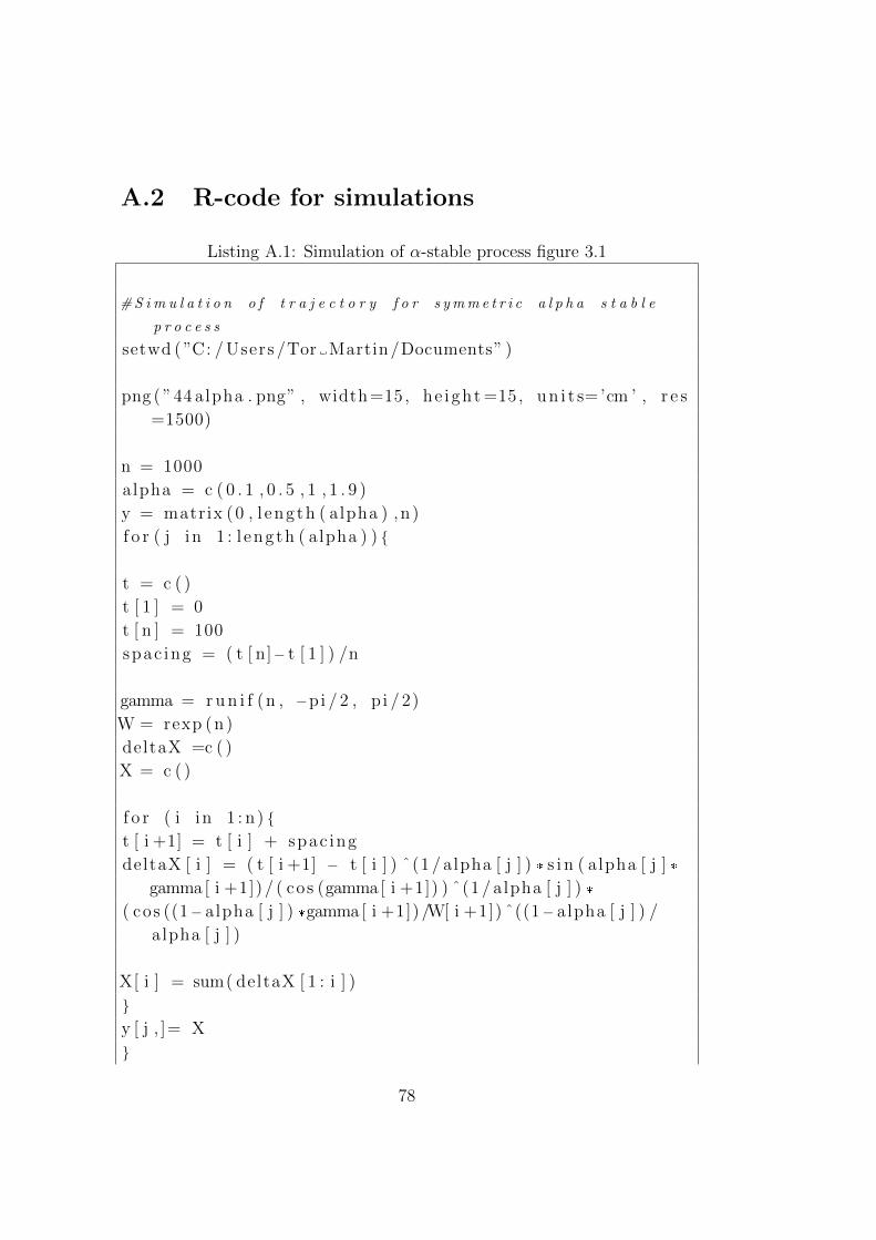
A.2 R-code for simulations

Listing A.1: Simulation of α-stable process figure 3.1

#S i m u l a t i o n o f t r a j e c t o r y f o r s ymm e t r i c a l p h a s t a b l e

p r o c e s s

setwd ( ”C: / Users /Tor Martin/Documents” )

png ( ”44 alpha . png” , width =15, he ight =15, un i t s=’cm ’ , r e s

=1500)

n = 1000

alpha = c ( 0 . 1 , 0 . 5 , 1 , 1 . 9 )

y = matrix (0 , l ength ( alpha ) ,n )

f o r ( j in 1 : l ength ( alpha ) )

t = c ( )

t [ 1 ] = 0

t [ n ] = 100

spac ing = ( t [ n]− t [ 1 ] ) /n

gamma = r u n i f (n , −pi / 2 , p i / 2)

W = rexp (n)

deltaX =c ( )

X = c ( )

f o r ( i in 1 : n ) t [ i +1] = t [ i ] + spac ing

deltaX [ i ] = ( t [ i +1] − t [ i ] ) ˆ(1 / alpha [ j ] ) * s i n ( alpha [ j ] *

gamma[ i +1]) / ( cos (gamma[ i +1]) ) ˆ(1 / alpha [ j ] ) *

( cos ((1− alpha [ j ] ) *gamma[ i +1]) /W[ i +1]) ˆ((1− alpha [ j ] ) /

alpha [ j ] )

X[ i ] = sum( deltaX [ 1 : i ] )

y [ j , ]= X

78

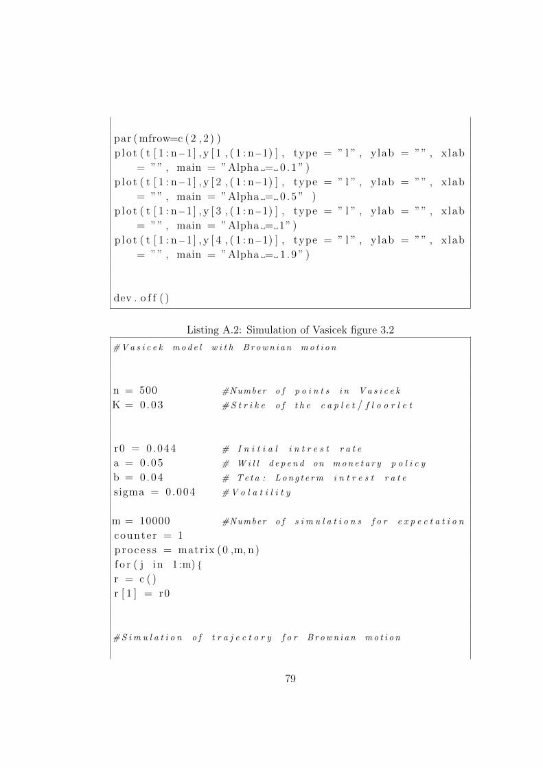
par ( mfrow=c (2 , 2 ) )

p l o t ( t [ 1 : n−1] , y [ 1 , ( 1 : n−1) ] , type = ” l ” , ylab = ”” , xlab

= ”” , main = ”Alpha = 0 .1 ” )

p l o t ( t [ 1 : n−1] , y [ 2 , ( 1 : n−1) ] , type = ” l ” , ylab = ”” , xlab

= ”” , main = ”Alpha = 0 .5 ” )

p l o t ( t [ 1 : n−1] , y [ 3 , ( 1 : n−1) ] , type = ” l ” , ylab = ”” , xlab

= ”” , main = ”Alpha = 1” )

p l o t ( t [ 1 : n−1] , y [ 4 , ( 1 : n−1) ] , type = ” l ” , ylab = ”” , xlab

= ”” , main = ”Alpha = 1 .9 ” )

dev . o f f ( )

Listing A.2: Simulation of Vasicek figure 3.2

#V a s i c e k mod e l w i t h B r own i an mo t i o n

n = 500 #Number o f p o i n t s i n V a s i c e k

K = 0.03 #S t r i k e o f t h e c a p l e t / f l o o r l e t

r0 = 0.044 # I n i t i a l i n t r e s t r a t e

a = 0.05 # W i l l d e p e n d on mon e t a r y p o l i c y

b = 0.04 # Te t a : L on g t e rm i n t r e s t r a t e

sigma = 0.004 #V o l a t i l i t y

m = 10000 #Number o f s i m u l a t i o n s f o r e x p e c t a t i o n

counter = 1

proce s s = matrix (0 ,m, n)

f o r ( j in 1 :m) r = c ( )

r [ 1 ] = r0

#S i m u l a t i o n o f t r a j e c t o r y f o r B r own i an mo t i o n

79

sigma BM = 0.1 #V o l a t i l a t y o f B r own i an mo t i o n

beta = 0 #D r i f t o f B r own i an mo t i o n

t = c ( )

t [ 1 ] = 0 #t 0 = t [ 1 ]

t [ n ] = 500

spac ing = ( t [ n]− t [ 1 ] ) / (n)

f o r ( i in 2 : ( n+1) ) t [ i ] = t [ i −1] + spac ing

N = rnorm (n)

deltaX = c ( )

L = c ( )

f o r ( i in 1 : n) deltaX [ i ] = sigma BM*N[ i ] * s q r t ( spac ing ) + beta * spac ing

L [ i ] = sum( deltaX [ 1 : i ] )

#V a s i c e k w i t h BM

de l t a t = spac ing

f o r ( i in 1 : ( n−1) ) dr = a * (b−r [ i ] ) * de l t a t + sigma * (L [ i +1]−L [ i ] )

r [ i +1] = r [ i ] + dr

proce s s [ j , ] = r

p r i n t ( counter )

counter = counter +1

expec ta t i on = c ( )

f o r ( i in 1 : n) expec ta t i on [ i ] = 1/m*sum( proce s s [ , i ] )

80

setwd ( ”C: / Users /Tor Martin/Documents” )

png ( ” va s i c ek run . png” , width =16, he ight =10, un i t s=’cm ’ ,

r e s =1500)

p l o t ( t [ 2 : ( n+1) ] , expectat ion , type = ” l ” , yl im = c

( 0 . 0 3 6 , 0 . 0 4 5 ) , x lab = ”Time” , ylab = ” r ” ,

main = ” Vasicek with a = 0 .05 , b = 0 .04 , r0 = 0.044 and

sigma = 0.004 ” , lwd = 2)

l i n e s ( t [ 2 : ( n+1) ] , p roc e s s [ 1 , ] , c o l = ” red ” )

l i n e s ( t [ 2 : ( n+1) ] , p roc e s s [ 2 , ] , c o l = ” blue ” )

l i n e s ( t [ 2 : ( n+1) ] , p roc e s s [ 3 , ] , c o l = ” green ” )

l i n e s ( t [ 2 : ( n+1) ] , p roc e s s [ 4 , ] , c o l = ” purple ” )

dev . o f f ( )

Listing A.3: Simulation of Vasicek figure 3.3

#V a s i c e k mod e l w i t h j ump s

n = 500 #Number o f p o i n t s i n V a s i c e k

r0 = 0.044 # I n i t i a l i n t r e s t r a t e

a = 0.05 # W i l l d e p e n d on mon e t a r y p o l i c y

b = 0.04 # Te t a : L on g t e rm i n t r e s t r a t e

sigma = 0.004 #V o l a t i l i t y

m = 10000 #Number o f s i m u l a t i o n s f o r e x p e c t a t i o n

counter = 1

proce s s = matrix (0 ,m, n)

f o r ( j in 1 :m) r = c ( )

r [ 1 ] = r0

81

#S i m u l a t i o n o f t r a j e c t o r y f o r s ymm e t r i c a l p h a s t a b l e

p r o c e s s

alpha = 1 .9

t = c ( )

t [ 1 ] = 0 #t 0 = t [ 1 ]

t [ n ] = 600

spac ing = ( t [ n]− t [ 1 ] ) / (n)

f o r ( i in 2 : ( n+1) ) t [ i ] = t [ i −1] + spac ing

gamma = r u n i f (n , −pi / 2 , p i / 2)

W = rexp (n)

deltaX =c ( )

deltaY = c ( )

L = c ( )

St = c ( )

f o r ( i in 1 : n ) deltaX [ i ] = ( spac ing ) ˆ(1 / alpha ) * ( s i n ( alpha *gamma[ i ] ) ) /

( ( cos (gamma[ i ] ) ) ˆ(1 / alpha ) ) *

( cos ((1− alpha ) *gamma[ i ] ) /W[ i ] ) ˆ((1− alpha ) / alpha )

deltaY [ i ] = ( spac ing ) ˆ(1 / ( 0 . 5 * alpha ) ) * ( s i n ( ( 0 . 5 * alpha ) *

gamma[ i ] ) ) / ( ( cos (gamma[ i ] ) ) ˆ(1 / ( 0 . 5 * alpha ) ) ) *

( cos ( (1 − (0 .5 * alpha ) ) *gamma[ i ] ) /W[ i ] ) ˆ((1 − (0 .5 * alpha ) ) /

( 0 . 5 * alpha ) )

L [ i ] = sum( deltaX [ 1 : i ] )

St [ i ] = sum( deltaY [ 1 : i ] )

82

#V a s i c e k w i t h j ump s

de l t a t = spac ing

f o r ( i in 1 : ( n−1) ) dr = a * (b−r [ i ] ) * de l t a t + sigma * (L [ i +1]−L [ i ] )

r [ i +1] = r [ i ] + dr

proce s s [ j , ] = r

p r i n t ( counter )

counter = counter +1

expec ta t i on = c ( )

f o r ( i in 1 : n) expec ta t i on [ i ] = 1/m*sum( proce s s [ , i ] )

setwd ( ”C: / Users /Tor Martin/Documents” )

png ( ” va s i c ek run jump . png” , width =16, he ight =10, un i t s=

’cm ’ , r e s =1500)

p l o t ( t [ 2 : ( n+1) ] , expectat ion , type = ” l ” , yl im = c

( 0 . 0 0 5 , 0 . 0 9 8 ) , xlab = ”Time” , ylab = ” r ” ,

main = ” Vasicek with a = 0 .05 , b = 0 .04 , r0 = 0.044 and

sigma = 0.004 ” , lwd = 2)

l i n e s ( t [ 2 : ( n+1) ] , p roc e s s [ 7 , ] , c o l = ” red ” )

dev . o f f ( )

83

\ begin l s t l i s t i n g [ frame = s i n g l e , capt ion = Simulat ion

o f f i g u r e \ r e f f i g : zhang ]

#V a s i c e k ( Zhang )

n = 600 #Number o f p o i n t s i n V a s i c e k

K = 0.05 #S t r i k e o f t h e c a p l e t ( s h o u l d b e h i g h e r t h e n

l o n g t e r m i n t e r e s t r a t e )

r0 = 0.048 # I n i t i a l i n t r e s t r a t e

a = 0.05 # W i l l d e p e n d on mon e t a r y p o l i c y

b = 0.04 # Te t a : L on g t e rm i n t r e s t r a t e

sigma = 0.004 #V o l a t i l i t y

m = 1000000 #Number o f s i m u l a t i o n s f o r e x p e c t a t i o n

counter = 1

proce s s = matrix (0 ,m, n)

f o r ( j in 1 :m) r = c ( )

r [ 1 ] = r0

#S i m u l a t i o n o f t r a j e c t o r y f o r s ymm e t r i c a l p h a s t a b l e

p r o c e s s

alpha = 0 .8

t = c ( )

t [ 1 ] = 0 #t 0 = t [ 1 ]

t [ n ] = 600

spac ing = ( t [ n]− t [ 1 ] ) / (n)

f o r ( i in 2 : ( n+1) ) t [ i ] = t [ i −1] + spac ing

84

gamma = r u n i f (n , −pi / 2 , p i / 2)

W = rexp (n)

deltaX =c ( )

deltaY = c ( )

L = c ( )

St = c ( )

f o r ( i in 1 : n ) deltaX [ i ] = ( spac ing ) ˆ(1 / alpha ) * ( s i n ( alpha *gamma[ i ] ) ) /

( ( cos (gamma[ i ] ) ) ˆ(1 / alpha ) ) *

( cos ((1− alpha ) *gamma[ i ] ) /W[ i ] ) ˆ((1− alpha ) / alpha )

deltaY [ i ] = ( spac ing ) ˆ(1 / ( 0 . 5 * alpha ) ) * ( s i n ( ( 0 . 5 * alpha ) *

gamma[ i ] ) ) / ( ( cos (gamma[ i ] ) ) ˆ(1 / ( 0 . 5 * alpha ) ) ) *

( cos ( (1 − (0 .5 * alpha ) ) *gamma[ i ] ) /W[ i ] ) ˆ((1 − (0 .5 * alpha ) ) /

( 0 . 5 * alpha ) )

L [ i ] = sum( deltaX [ 1 : i ] )

St [ i ] = sum( deltaY [ 1 : i ] )

#V a s i c e k w i t h j ump s

de l t a t = spac ing

f o r ( i in 1 : ( n−1) ) dr = a * (b−r [ i ] ) * de l t a t + sigma * (L [ i +1]−L [ i ] )

r [ i +1] = r [ i ] + dr

t = t [ 2 : ( n+1) ]

#S t o c h a s t i c i n t e g r a l p a r t

s to i n t = c ( )

85

s to i n t s = c ( )

f o r ( i in 1 : ( l ength ( t ) −1) ) s to i n t [ i ] = exp(−a * t [ i ] ) * (L [ i +1]−L [ i ] )

s to i n t s [ i ] = sum( s to i n t [ 1 : i ] )

s to i n t s

#Main e x p r e s s i o n

r1 = pmax( r−K, 0 )

va lue s = c ( )

f o r ( i in 1 : l ength ( t ) ) va lue s [ i ] = 1/St [ i ] * r1 [ i ] * s to i n t s [ i ] *1/sigma

pr in t ( counter )

counter = counter + 1

proce s s [ j , ] = va lue s

expec ta t i on = c ( )

f o r ( i in 1 : n) expec ta t i on [ i ] = 1/m*sum( proce s s [ , i ] )

setwd ( ”C: / Users /Tor Martin/Documents” )

png ( ”zhang0 8 . png” , width =16, he ight =10, un i t s=’cm ’ ,

r e s =1000)

86

p lo t ( t [ 1 : ( n−1) ] , expec ta t i on [ 1 : ( n−1) ] , type = ” l ” , xlim =

c (0 , t [ n ] ) , yl im = c (−5 ,5) , x lab = ”Time” ,

ylab = ” Expectat ion ” , main = ” r0 = 0 .048 , s t r i k e =

0 .05 , longterm i n t e r e s t r a t e = 0 .04 ” )

l i n e s ( t [ 1 : ( n−1) ] , expectationBM [ 1 : ( n−1) ] , c o l = ” red ” )

dev . o f f ( )

Listing A.4: Simulation of figure 3.5 (Brownian motion added to figure 3.4)

#V a s i c e k ( Zhang ) i n t h e c a s e o f B r own i a n mo t i o n

setwd ( ”C: / Users /Tor Martin/Documents” )

#png ( ” z h a n g 1 BM. png ” , w i d t h =16 , h e i g h t =10 , u n i t s = ’cm ’ ,

r e s =1000 )

n = 600 #Number o f p o i n t s i n V a s i c e k

K = 0.05 #S t r i k e o f t h e c a p l e t

r0 = 0.048 # I n i t i a l i n t r e s t r a t e

a = 0.05 # W i l l d e p e n d on mon e t a r y p o l i c y

b = 0.04 # Te t a : L on g t e rm i n t r e s t r a t e

sigma = 0.004 #V o l a t i l i t y

m = 10000 #Number o f s i m u l a t i o n s f o r e x p e c t a t i o n

counter = 1

proce s s = matrix (0 ,m, n)

f o r ( j in 1 :m) r = c ( )

r [ 1 ] = r0

#S i m u l a t i o n o f t r a j e c t o r y f o r B r own i an mo t i o n

87

sigma BM = 0.5 #V o l a t i l a t y o f B r own i an mo t i o n

b = 0.06 #D r i f t o f B r own i an mo t i o n

t = c ( )

t [ 1 ] = 0 #t 0 = t [ 1 ]

t [ n ] = 600

spac ing = ( t [ n]− t [ 1 ] ) / (n)

f o r ( i in 2 : ( n+1) ) t [ i ] = t [ i −1] + spac ing

N = rnorm (n)

deltaX = c ( )

L = c ( )

f o r ( i in 1 : n) deltaX [ i ] = sigma BM*N[ i ] * s q r t ( spac ing ) + b* spac ing

L [ i ] = sum( deltaX [ 1 : i ] )

#V a s i c e k w i t h BM

de l t a t = spac ing

f o r ( i in 1 : ( n−1) ) dr = a * (b−r [ i ] ) * de l t a t + sigma * (L [ i +1]−L [ i ] )

r [ i +1] = r [ i ] + dr

t = t [ 2 : ( n+1) ]

#p l o t ( t , r , t y p e = ” l ” )

# S t o c h a s t i c i n t e g r a l p a r t

s to i n t = c ( )

s to i n t s = c ( )

88

f o r ( i in 1 : ( l ength ( t ) −1) ) s to i n t [ i ] = exp(−a * t [ i ] ) * (L [ i +1]−L [ i ] )

s to i n t s [ i ] = sum( s to i n t [ 1 : i ] )

s to i n t s

#Main e x p r e s s i o n

r1 = pmax( r−K, 0 )

va lue s = c ( )

f o r ( i in 1 : l ength ( t ) ) va lue s [ i ] = 1/ t [ i ] * r1 [ i ] * s to i n t s [ i ] *1/sigma

pr in t ( counter )

counter = counter + 1

proce s s [ j , ] = va lue s

expectationBM = c ( )

f o r ( i in 1 : n) expectationBM [ i ] = 1/m*sum( proce s s [ , i ] )

setwd ( ”C: / Users /Tor Martin/Documents” )

png ( ”zhang1 BM f i n a l . png” , width =16, he ight =10, un i t s=’

cm ’ , r e s =1000)

89

p lo t ( t [ 1 : ( n−1) ] , expectationBM [ 1 : ( n−1) ] , type = ” l ” , xlim

= c (0 , t [ n ] ) , yl im = c (−5 ,5) , xlab = ”Time” , ylab =

” Expectat ion ” )

l i n e s ( t [ 1 : ( n−1) ] , expectationBM [ 1 : ( n−1) ] , c o l = ” red ” )

dev . o f f ( )

Listing A.5: Simulation of figure 3.6

#Endowment p o l i c y w i t h j ump s

m = 200000 #Number o f s i m u l a t i o n s f o r e x p e c t a t i o n

K = 0.05 #S t r i k e o f t h e c a p l e t ( s h o u l d b e h i g h e r

t h e n l o n g t e r m i n t e r e s t r a t e )

de l t a = 0.03 #F i x e d i n t e r e s t r a t e o v e r t h e p e r i o d e

o f t h e c o n t r a c t

s = 35 #Age o f t h e i n d i v i d u a l a t t h e b e g i n n i n g

o f t h e c o n t r a c t

T = 65 #Age o f t h e i n d i v i d u a l a t t h e end o f

t h e c o n t r a c t

k = 12 #Number o f o b s e r e v e d i n t e r e s t r a t e

c h a n g e s p e r y e a r e . g . 12 i f c h a n g e e v e r y month

n = (T−s ) *k #Number o f p o i n t s o v e r t h e t o t a l p e r i o d

r0 = 0.048 # I n i t i a l i n t r e s t r a t e

a = 0.05 #W i l l d e p e n d on mon e t a r y p o l i c y

b = 0.04 #Te t a : L on g t e rm i n t r e s t r a t e

sigma = 0.004 #V o l a t i l i t y

#T r a n s i t i o n p r o b a b i l i t i e s

aa = −7.85785

bb = 0.01538

cc = 5.77355 * 10ˆ(−4)

90

uxt = func t i on ( x ) exp ( aa+bb*x+cc *xˆ2)

pxx = func t i on ( s ,T) exp (−( i n t e g r a t e ( uxt , s ,T) $ value ) )

counter = 1

proce s s = matrix (0 ,m, n)

f o r ( j in 1 :m) r = c ( )

r [ 1 ] = r0

#S i m u l a t i o n o f t r a j e c t o r y f o r s ymm e t r i c a l p h a s t a b l e

p r o c e s s

alpha = 1 .9

t = c ( )

t [ 1 ] = 0 #t 0 = t [ 1 ]

t [ n ] = (T−s ) * 365

spac ing = ( t [ n]− t [ 1 ] ) / (n)

f o r ( i in 2 : ( n+1) ) t [ i ] = t [ i −1] + spac ing

gamma = r u n i f (n , −pi / 2 , p i / 2)

W = rexp (n)

deltaX =c ( )

deltaY = c ( )

L = c ( )

St = c ( )

f o r ( i in 1 : n )

91

deltaX [ i ] = ( spac ing ) ˆ(1 / alpha ) * ( s i n ( alpha *gamma[ i ] ) ) /

( ( cos (gamma[ i ] ) ) ˆ(1 / alpha ) ) *

( cos ((1− alpha ) *gamma[ i ] ) /W[ i ] ) ˆ((1− alpha ) / alpha )

deltaY [ i ] = ( spac ing ) ˆ(1 / ( 0 . 5 * alpha ) ) * ( s i n ( ( 0 . 5 * alpha ) *

gamma[ i ] ) ) / ( ( cos (gamma[ i ] ) ) ˆ(1 / ( 0 . 5 * alpha ) ) ) *

( cos ( (1 − (0 .5 * alpha ) ) *gamma[ i ] ) /W[ i ] ) ˆ((1 − (0 .5 * alpha ) ) /

( 0 . 5 * alpha ) )

L [ i ] = sum( deltaX [ 1 : i ] )

St [ i ] = sum( deltaY [ 1 : i ] )

#V a s i c e k w i t h j ump s

de l t a t = spac ing

f o r ( i in 1 : ( n−1) ) dr = a * (b−r [ i ] ) * de l t a t + sigma * (L [ i +1]−L [ i ] )

r [ i +1] = r [ i ] + dr

t = t [ 2 : ( n+1) ]

#S t o c h a s t i c i n t e g r a l p a r t

s to i n t = c ( )

s to i n t s = c ( )

f o r ( i in 1 : ( l ength ( t ) −1) ) s to i n t [ i ] = exp(−a * t [ i ] ) * (L [ i +1]−L [ i ] )

s to i n t s [ i ] = sum( s to i n t [ 1 : i ] )

#s t o i n t s

92

#Main e x p r e s s i o n

r1 = pmax( r−K, 0 )

va lue s = c ( )

f o r ( i in 1 : l ength ( t ) ) va lue s [ i ] = 1/St [ i ] * r1 [ i ] * s to i n t s [ i ] *1/sigma

pr in t ( counter )

counter = counter + 1

proce s s [ j , ] = va lue s

expec ta t i on = c ( )

f o r ( i in 1 : n) expec ta t i on [ i ] = 1/m*sum( proce s s [ , i ] )

V0 = exp(− de l t a * (T−s ) ) * expec ta t i on *pxx ( s ,T)

setwd ( ”C: / Users /Tor Martin/Documents” )

png ( ”endowment 1 8 . png” , width =16, he ight =10, un i t s=’cm

’ , r e s =1000)

p l o t ( ( t [ 1 : ( n−1) ] / 365) ,V0 [ 1 : ( n−1) ] , type = ” l ” , yl im = c

( −0 .2 , 0 . 3 ) , x lab = ”Time” ,

ylab = ”” , main = ” S e n s i t i v i t y o f an endowment p o l i c y ” )

93

dev . o f f ( )

Listing A.6: Simulation of figure 3.7

#Endowment p o l i c y w i t h B r own i an mo t i o n

m = 10000 #Number o f s i m u l a t i o n s f o r e x p e c t a t i o n

K = 0.05 #S t r i k e o f t h e c a p l e t ( s h o u l d b e h i g h e r

t h e n l o n g t e r m i n t e r e s t r a t e )

de l t a = 0.03 #F i x e d i n t e r e s t r a t e o v e r t h e p e r i o d e

o f t h e c o n t r a c t

s = 35 #Age o f t h e i n d i v i d u a l a t t h e b e g i n n i n g

o f t h e c o n t r a c t

T = 65 #Age o f t h e i n d i v i d u a l a t t h e end o f

t h e c o n t r a c t

k = 12 #Number o f o b s e r e v e d i n t e r e s t r a t e

c h a n g e s p e r y e a r e . g . 12 i f c h a n g e e v e r y month

n = (T−s ) *k #Number o f p o i n t s o v e r t h e t o t a l p e r i o d

r0 = 0.048 # I n i t i a l i n t r e s t r a t e

a = 0.05 #W i l l d e p e n d on mon e t a r y p o l i c y

b = 0.04 #Te t a : L on g t e rm i n t r e s t r a t e

sigma = 0.004 #V o l a t i l i t y

#T r a n s i t i o n p r o b a b i l i t i e s

aa = −7.85785

bb = 0.01538

cc = 5.77355 * 10ˆ(−4)

uxt = func t i on ( x ) exp ( aa+bb*x+cc *xˆ2)

pxx = func t i on ( s ,T) exp (−( i n t e g r a t e ( uxt , s ,T) $ value ) )

94

counter = 1

proce s s = matrix (0 ,m, n)

f o r ( j in 1 :m) r = c ( )

r [ 1 ] = r0

#S i m u l a t i o n o f t r a j e c t o r y f o r B r own i an mo t i o n

sigma BM = 0.5 #V o l a t i l a t y o f B r own i an mo t i o n

bbb = 0.06 #D r i f t o f B r own i an mo t i o n

t = c ( )

t [ 1 ] = 0 #t 0 = t [ 1 ]

t [ n ] = (T−s ) * 365

spac ing = ( t [ n]− t [ 1 ] ) / (n)

f o r ( i in 2 : ( n+1) ) t [ i ] = t [ i −1] + spac ing

N = rnorm (n)

deltaX = c ( )

L = c ( )

f o r ( i in 1 : n) deltaX [ i ] = sigma BM*N[ i ] * s q r t ( spac ing ) + bbb* spac ing

L [ i ] = sum( deltaX [ 1 : i ] )

#V a s i c e k w i t h j ump s

de l t a t = spac ing

f o r ( i in 1 : ( n−1) )

95

dr = a * (b−r [ i ] ) * de l t a t + sigma * (L [ i +1]−L [ i ] )

r [ i +1] = r [ i ] + dr

t = t [ 2 : ( n+1) ]

#S t o c h a s t i c i n t e g r a l p a r t

s to i n t = c ( )

s to i n t s = c ( )

f o r ( i in 1 : ( l ength ( t ) −1) ) s to i n t [ i ] = exp(−a * t [ i ] ) * (L [ i +1]−L [ i ] )

s to i n t s [ i ] = sum( s to i n t [ 1 : i ] )

#s t o i n t s

#Main e x p r e s s i o n

r1 = pmax( r−K, 0 )

va lue s = c ( )

f o r ( i in 1 : l ength ( t ) ) va lue s [ i ] = 1/ t [ i ] * r1 [ i ] * s to i n t s [ i ] *1/sigma

pr in t ( counter )

counter = counter + 1

proce s s [ j , ] = va lue s

expec ta t i on = c ( )

f o r ( i in 1 : n)

96

expec ta t i on [ i ] = 1/m*sum( proce s s [ , i ] )

V0 = exp(− de l t a * (T−s ) ) * expec ta t i on *pxx ( s ,T)

setwd ( ”C: / Users /Tor Martin/Documents” )

png ( ”endowment BM. png” , width =16, he ight =10, un i t s=’cm ’

, r e s =1000)

p l o t ( ( t [ 1 : ( n−1) ] / 365) ,V0 [ 1 : ( n−1) ] , type = ” l ” , yl im = c

( −0 .0003 ,0 .0042) , xlab = ”Time” ,

ylab = ”” , main = ” S e n s i t i v i t y o f an endowment p o l i c y

with BM” )

# l i n e s ( t [ 1 : ( n−1) ] , e x p e c t a t i o n BM [ 1 : ( n−1) ] , c o l = ” r e d ” )

dev . o f f ( )

Listing A.7: Simulation of figure 3.8

#Term l i f e i n s u r a n c e w i t h j ump s

m = 100000 #Number o f s i m u l a t i o n s f o r

e x p e c t a t i o n

de l t a = 0.03 #F i x e d i n t e r e s t r a t e o v e r t h e p e r i o d e

o f t h e c o n t r a c t

s = 35 #Age o f t h e i n d i v i d u a l a t t h e b e g i n n i n g

o f t h e c o n t r a c t

T = 65 #Age o f t h e i n d i v i d u a l a t t h e end o f

t h e c o n t r a c t

k = 12 #Number o f o b s e r e v e d i n t e r e s t r a t e

c h a n g e s p e r y e a r e . g . 12 i f c h a n g e e v e r y month

97

n = (T−s ) *k #Number o f p o i n t s o v e r t h e t o t a l p e r i o d

x0 = 6 # I n i t i a l v a l u e o f s t o c k

sigma = 0 .5 #V o l a t i l i t y

G = 5 #Gu a r a n t e e

K = 8 #S t r i k e p r i c e

#T r a n s i t i o n p r o b a b i l i t i e s

aa = −7.85785

bb = 0.01538

cc = 5.77355 * 10ˆ(−4)

uxt = func t i on ( x ) exp ( aa+bb*x+cc *xˆ2)

pxx = func t i on ( s ,T) exp (−( i n t e g r a t e ( uxt , s ,T) $ value ) )

counter = 1

proce s s = matrix (0 ,m, n)

f o r ( j in 1 :m)

#S i m u l a t i o n o f t r a j e c t o r y f o r s ymm e t r i c a l p h a s t a b l e

p r o c e s s

alpha = 1 .9

t = c ( )

t [ 1 ] = 0 #t 0 = t [ 1 ]

t [ n ] = (T−s ) * 365

spac ing = ( t [ n]− t [ 1 ] ) / (n)

f o r ( i in 2 : ( n+1) )

98

t [ i ] = t [ i −1] + spac ing

gamma = r u n i f (n , −pi / 2 , p i / 2)

W = rexp (n)

deltaX =c ( )

deltaY = c ( )

L = c ( )

St = c ( )

f o r ( i in 1 : n ) deltaX [ i ] = ( spac ing ) ˆ(1 / alpha ) * ( s i n ( alpha *gamma[ i ] ) ) /

( ( cos (gamma[ i ] ) ) ˆ(1 / alpha ) ) *

( cos ((1− alpha ) *gamma[ i ] ) /W[ i ] ) ˆ((1− alpha ) / alpha )

deltaY [ i ] = ( spac ing ) ˆ(1 / ( 0 . 5 * alpha ) ) * ( s i n ( ( 0 . 5 * alpha ) *

gamma[ i ] ) ) / ( ( cos (gamma[ i ] ) ) ˆ(1 / ( 0 . 5 * alpha ) ) ) *

( cos ( (1 − (0 .5 * alpha ) ) *gamma[ i ] ) /W[ i ] ) ˆ((1 − (0 .5 * alpha ) ) /

( 0 . 5 * alpha ) )

L [ i ] = sum( deltaX [ 1 : i ] )

St [ i ] = sum( deltaY [ 1 : i ] )

L = L/max( abs (L) )

St = St/max( abs (L) )

t = t [ 2 : ( n+1) ]

#S t o c h a s t i c i n t e g r a l p a r t

s to i n t = c ( )

s to i n t s = c ( )

f o r ( i in 1 : ( l ength ( t ) −1) ) s to i n t [ i ] = exp ( sigma *L [ i ] ) * (L [ i +1]−L [ i ] )

99

s to i n t s [ i ] = sum( s to i n t [ 1 : i ] )

#s t o i n t s

#Main e x p r e s s i o n

r1 = pmax(K−x0 * exp ( sigma *L) ,G)

va lue s = c ( )

f o r ( i in 1 : l ength ( t ) ) va lue s [ i ] = 1/St [ i ] * r1 [ i ] * s to i n t s [ i ] *1/sigma

pr in t ( counter )

counter = counter + 1

proce s s [ j , ] = va lue s

expec ta t i on = c ( )

f o r ( i in 1 : n) expec ta t i on [ i ] = 1/m*sum( proce s s [ , i ] )

de l t a t = spac ing

i n t V0 = c ( )

V0 = c ( )

f o r ( i in 1 : l ength ( t ) ) i n t V0 [ i ] = exp(− de l t a * ( t [ i ] / 365) ) * expec ta t i on [ i ] *pxx ( s

, s+(t [ i ] / 365) ) * uxt ( s+t [ i ] / 365) * ( d e l t a t / 365)

V0 [ i ] = sum( i n t V0 [ 1 : i ] )

100

setwd ( ”C: / Users /Tor Martin/Documents” )

png ( ”term l i f e 6 1 9 . png” , width =16, he ight =10, un i t s=’

cm ’ , r e s =1000)

p l o t ( ( t [ 1 : ( n−1) ] / 365) ,V0 [ 1 : ( n−1) ] , type = ” l ” , xlab = ”

Time” ,

ylab = ”” , main = ”” )

dev . o f f ( )

Listing A.8: Simulation of figure 3.9

#Term l i f e i n s u r a n c e w i t h B r own i an mo t i o n

m = 100000 #Number o f s i m u l a t i o n s f o r e x p e c t a t i o n

de l t a = 0.03 #F i x e d i n t e r e s t r a t e o v e r t h e p e r i o d e

o f t h e c o n t r a c t

s = 35 #Age o f t h e i n d i v i d u a l a t t h e b e g i n n i n g

o f t h e c o n t r a c t

T = 65 #Age o f t h e i n d i v i d u a l a t t h e end o f

t h e c o n t r a c t

k = 12 #Number o f o b s e r e v e d i n t e r e s t r a t e

c h a n g e s p e r y e a r e . g . 12 i f c h a n g e e v e r y month

n = (T−s ) *k #Number o f p o i n t s o v e r t h e t o t a l p e r i o d

x0 = 20 # I n i t i a l v a l u e o f s t o c k

sigma = 0 .5 #V o l a t i l i t y

G = 20 #Gu a r a n t e e

K = 50 #S t r i k e p r i c e

#T r a n s i t i o n p r o b a b i l i t i e s

aa = −7.85785

101

bb = 0.01538

cc = 5.77355 * 10ˆ(−4)

uxt = func t i on ( x ) exp ( aa+bb*x+cc *xˆ2)

pxx = func t i on ( s ,T) exp (−( i n t e g r a t e ( uxt , s ,T) $ value ) )

counter = 1

proce s s = matrix (0 ,m, n)

f o r ( j in 1 :m)

#S i m u l a t i o n o f t r a j e c t o r y f o r B r own i an mo t i o n

sigma BM = 0.5 #V o l a t i l a t y o f B r own i an mo t i o n

bbb = 0 .1 #D r i f t o f B r own i an mo t i o n

t = c ( )

t [ 1 ] = 0 #t 0 = t [ 1 ]

t [ n ] = (T−s ) * 365

spac ing = ( t [ n]− t [ 1 ] ) / (n)

f o r ( i in 2 : ( n+1) ) t [ i ] = t [ i −1] + spac ing

N = rnorm (n)

deltaX = c ( )

L = c ( )

f o r ( i in 1 : n) deltaX [ i ] = sigma BM*N[ i ] * s q r t ( spac ing ) + bbb* spac ing

L [ i ] = sum( deltaX [ 1 : i ] )

102

L = L/ (max( abs (L) ) )

t = t [ 2 : ( n+1) ]

#S t o c h a s t i c i n t e g r a l p a r t

s to i n t = c ( )

s to i n t s = c ( )

f o r ( i in 1 : ( l ength ( t ) −1) ) s to i n t [ i ] = exp ( sigma *L [ i ] ) * (L [ i +1]−L [ i ] )

s to i n t s [ i ] = sum( s to i n t [ 1 : i ] )

#s t o i n t s

#Main e x p r e s s i o n

r1 = pmax(K−x0 * exp ( sigma *L) ,G)

va lue s = c ( )

f o r ( i in 1 : l ength ( t ) ) va lue s [ i ] = 1/ t [ i ] * r1 [ i ] * s to i n t s [ i ] *1/sigma

pr in t ( counter )

counter = counter + 1

proce s s [ j , ] = va lue s

expec ta t i on = c ( )

f o r ( i in 1 : n) expec ta t i on [ i ] = 1/m*sum( proce s s [ , i ] )

103

de l t a t = spac ing

i n t V0 = c ( )

V0 = c ( )

f o r ( i in 1 : l ength ( t ) ) i n t V0 [ i ] = exp(− de l t a * ( t [ i ] / 365) ) * expec ta t i on [ i ] *pxx ( s

, s+(t [ i ] / 365) ) * uxt ( s+t [ i ] / 365) * ( d e l t a t / 365)

V0 [ i ] = sum( i n t V0 [ 1 : i ] )

#s e t w d ( ”C : / U s e r s /Tor Ma r t i n / Documen t s ” )

#png ( ” t e rm l i f e BM. png ” , w i d t h =16 , h e i g h t =10 , u n i t s = ’cm

’ , r e s =1000 )

p lo t ( ( t [ 1 : ( n−1) ] / 365) ,V0 [ 1 : ( n−1) ] , type = ” l ” , xlab = ”

Time” ,

ylab = ”” , main = ”” )

# l i n e s ( t [ 1 : ( n−1) ] , e x p e c t a t i o n BM [ 1 : ( n−1) ] , c o l = ” r e d ” )

#d e v . o f f ( )

A.3 Bibliography

104

Bibliography

[1] Benth, Fred E.: Option Theory with Stochastic Analysis: An

Introduction to Mathematical Finance. Springer (2004).

[2] Brigo, D., Mercurio, F.: Interest Rate Models - Theory and

Practice 2nd edition. Springer (2006).

[3] Cont, R., Tankov, R.: Financial modelling with jump processes.

Chapman & Hall (2004).

[4] Di Nunno, Øksendal, B., Proske, F.: Malliavin Calculus for

Levy Processes with application to Finance. Springer (2008).

[5] Evans, Lawrence C.: Partial Differential Equations, 2nd edition.

American Mathematical Society (2010).

[6] Fournie, E. Lasry, J.-M., Lebuchoux, J., Lions, P.-L, Touzi, N.:

Applications of Malliavin Calculus to Monte Carlo methods in

finance. Finance Stoch., 3(4) : 391− 412(1999).

[7] Fournie, E. Lasry, J.-M., Lebuchoux, J., Lions, P.-L, Touzi, N.:

Applications of Malliavin Calculus to Monte Carlo methods in

finance Π . Finance Stoch., 5(2) : 201− 236(2001).

[8] Haadem, S. ,Proske, F.: On the construction and Malliavin

differentiability of solutions of Levy noise driven SDE’s with

singular coefficients. Journal of functional analysis, 266, 5321−5359 (2014).

[9] Ikeda, N., Watanabe, S.: Stochastic Differential Equations and

Diffusion Processes, 2nd edition. North-Holland Mathematical

Library (1989).

105

[10] Jackel, P.: Monte Carlo Methods in Finance. John Wiley &

Sons, Chichester (2002).

[11] Koller, M.: Stochastic Models in Life Insurance. Springer

(2011).

[12] Meneoukeu-Pamen, O., Meyer-Brandis, T., Nilssen, T.,

Proske,F., Zhang, T.: A variational approach to the construc-

tion and Malliavin differentiability of strong solutions of SDE’s.

Springer (2013).

[13] Peszat, S. , Zabczyk, J. : Stochastic Partial Differential Equa-

tions with Levy Noise. Cambridge university press (2007).

[14] Protter, P.: Stochastic integration and differential equations,

2nd edition, Springer (2005).

[15] Rynne, B. ,Youngson, M.: Linear Functional Analysis, 2nd edi-

tion. Springer (2008).

[16] Veretennikov, A. Yu.: On strong solutions of Ito equations with

jumps. Theory Probab. Appl., 32(1), 148− 152(1985).

[17] Zhang, X.: Derivative formulas and gradient estimates for

SDE’s driven by α-stable processes. Stochastic Processes and

Their Applications 123 p.1213-1228 (2012).

[18] Øksendal,B.: Stochastic Differential Equations. Springer

(2010).

[19] Øksendal, B., Sulem ,A.: Applied Stochastic Control of Jump

Diffusions. Springer (2007).

106