5 The Dirac Equation and Spinors

In this section we develop the appropriate wavefunctions for fundamental fermions andbosons.

5.1 Notation Review

The three dimension differential operator is :

=

∂

∂x,

∂

∂y,

∂

∂z

(5.1)

We can generalise this to four dimensions ∂µ:

∂µ =

1

c

∂

∂t,

∂

∂x,

∂

∂y,

∂

∂z

(5.2)

5.2 The Schrodinger Equation

First consider a classical non-relativistic particle of mass m in a potential U . Theenergy-momentum relationship is:

E =p

2

2m+ U (5.3)

we can substitute the differential operators:

E → i ∂

∂tp→ −i (5.4)

to obtain the non-relativistic Schrodinger Equation (with = 1):

i∂ψ

∂t=

−

1

2m2 + U

ψ (5.5)

For U = 0, the free particle solutions are:

ψ(x, t) ∝ e−iEt

ψ(x) (5.6)

and the probability density ρ and current j are given by:

ρ = |ψ(x)|2 j = −i

2m

ψ∗ψ − ψψ

∗ (5.7)

with conservation of probability giving the continuity equation:

∂ρ

∂t+ ·j = 0, (5.8)

Or in Covariant notation:

∂µjµ = 0 with j

µ = (ρ,j) (5.9)

The Schrodinger equation is 1st order in ∂/∂t but second order in ∂/∂x. However, aswe are going to be dealing with relativistic particles, space and time should be treatedequally.

25

5.3 The Klein-Gordon Equation

For a relativistic particle the energy-momentum relationship is:

p · p = pµpµ = E

2− |p|

2 = m2 (5.10)

Substituting the equation (5.4), leads to the relativistic Klein-Gordon equation:−

∂2

∂t2+ 2

ψ = m

2ψ (5.11)

The free particle solutions are plane waves:

ψ ∝ e−ip·x = e

−i(Et−p·x) (5.12)

The Klein-Gordon equation successfully describes spin 0 particles in relativistic quan-tum field theory.

There are problems with the interpretation of the positive and negative energy solutionsof the Klein-Gordon equation, E = ±

p2 + m2, since the negative energy solutions

have negative probability densities ρ.

5.4 The Dirac Equation

The problems with the Klein-Gordon equation led Dirac to search for an alternativerelativistic wave equation in 1928, in which the time and space derivatives are firstorder. The Dirac equation can be thought of in terms of a “square root” of theKlein-Gordon equation. In covariant form it is written:

iγ

0 ∂

∂t+ iγ · −m

ψ = 0 (iγµ

∂µ −m) ψ = 0 (5.13)

where we have introduced the coefficients γµ = (γ0

,γ) = (γ0, γ

1, γ

2, γ

3), which have tobe determined.

As we will see in equation (5.20), the Dirac equation is simply four coupled differentialequations, describing a wavefunction ψ with four components.

5.5 The Gamma Matrices

To find what the γµ, µ = 0, 1, 2, 3 objects are, we first multiply the Dirac equation by

its conjugate equation:

ψ†−iγ

0 ∂

∂t− iγ · −m

iγ

0 ∂

∂t+ iγ · −m

ψ = 0 (5.14)

and demand that this be consistent with the Klein-Gordon equation, (5.11). This leadsto the following conditions on the γ

µ:

(γ0)2 = 1, (γi)2 = −1 γµγ

ν + γνγ

µ = 0 for µ = ν

with i = 1, 2, 3, µ, ν = 0, 1, 2, 3 (5.15)

26

Equivalently in terms of anticommutation relations and the metric tensor (equation (3.3)):

γµ, γ

ν = γ

µ, γ

ν + γν, γ

µ = 2gµνµ, ν = 0, 1, 2, 3 (5.16)

The simplest solution for the γµ, that satisfies these anticommutation relations, are

4× 4 unitary matrices. We will use the following representation for the γ matrices:

γ0 =

I 00 −I

γ

i =

0 σ

i

−σi 0

(5.17)

where I denotes a 2× 2 identity matrix, 0 denotes a 2× 2 null matrix, and the σi are

the Pauli spin matrices:

σx =

0 11 0

σy =

0 −i

i 0

σz =

1 00 −1

(5.18)

Let’s write out the gamma matrices in full:

γ0 =

1 0 0 00 1 0 00 0 −1 01 0 0 −1

γ1 =

0 0 0 10 0 1 00 −1 0 0−1 0 0 0

γ2 =

0 0 0 −i

0 0 i 00 i 0 0−i 0 0 0

γ3 =

0 0 1 00 0 0 −1−1 0 0 00 1 0 0

(5.19)

Please note, despite the µ superscript, the γµ are not four vectors. However they do

remain constant under Lorentz transforms.

Finally let’s write out the Dirac Equation in full:

i∂∂t −m 0 i

∂∂z i

∂∂x + ∂

∂y

0 i∂∂t −m i

∂∂x −

∂∂y −i

∂∂z

−i∂∂z −i

∂∂x −

∂∂y −i

∂∂t −m 0

−i∂∂x + ∂

∂y i∂∂z 0 −i

∂∂t −m

ψ1

ψ2

ψ3

ψ4

=

0000

(5.20)

5.6 Spinors

The Dirac equation describes the behaviour of spin-1/2 fermions in relativistic quantumfield theory. For a free fermion the wavefunction is the product of a plane wave and aDirac spinor, u(pµ):

ψ(xµ) = u(pµ)e−ip·x (5.21)

Substituting the fermion wavefunction, ψ, into the Dirac equation:

(γµpµ −m)u(p) = 0 (5.22)

27

For a particle at rest, p = 0, we find the following equations:

iγ0 ∂

∂t−m

ψ =

γ

0E −m

ψ = 0 E u =

mI 00 −mI

u (5.23)

The solutions are four eigenspinors:

u1 =

1000

u2 =

0100

u3 =

0010

u4 =

0001

(5.24)

and the associated wavefunctions of the fermion is:

ψ1 = e

−imtu

1ψ

2 = e−imt

u2

ψ3 = e

+imtu

3ψ

4 = e+imt

u4 (5.25)

Note that the spinors are 1 × 4 column matrices, and that there are four possiblestates. The spinors are, however, not four-vectors: the four components do not representt, x, y, z.

The four components are a suprise: we would expect only two spin states for a spin-1/2fermion! Note also the change of sign in the exponents of the plane waves in the statesψ

3 and ψ4. The four solutions in equations (5.24) and (5.25) describe two different spin

states (↑ and ↓) with E = m, and two spin states with E = −m.

5.7 Negative Energy Solutions & Antimatter

To describe the negative energy states, Dirac postulated that an electron in a positiveenergy state is produced from the vacuum accompanied by a hole with negative energy.The hole corresponds to a physical antiparticle, the positron, with charge +e.

Another interpretation (Feynman-Stuckelberg) is that the E = −m solutions can eitherdescribe a negative energy particle which propagates backwards in time, or a positiveenergy antiparticle propagating forward in time:

e−i[(−E)(−t)−(−p)·(−x)] = e

−i[Et−p·x] (5.26)

5.8 Spinors for Moving Particles

For a moving particle, p = 0 the Dirac equation becomes (using (5.13) and (5.17)):

(γµpµ −m)

uA uB

=

E −m −σ · p

σ · p −E −m

uA

uB

= 0 (5.27)

where uA and uB denote the 1× 2 upper and lower components of u respectively. Theequations for uA and uB are coupled:

uA =σ · p

E −muB uB =

σ · p

E + muA (5.28)

28

The solutions are obtained by successively setting: uA =

10

, uA =

01

, uB =

10

, and uB =

01

, to give:

u1 =

10

pz/(E + m)(px + ipy)/(E + m)

u2 =

01

(px − ipy)/(E + m)−pz/(E + m)

u3 =

−pz/(−E + m)(−px − ipy)/(−E + m)

10

u4 =

(−px + ipy)/(−E + m)pz/(−E + m)

01

(5.29)

The u1 and u

2 solutions describe an electron of energy E = +

m2 + p 2, and momen-tum p:

ψ = u1(pµ)e−ip·x

ψ = u2(pµ)e−ip·x (5.30)

The u3 and u

4 of equation (5.29) describe a positron of energy E = −

m2 + p 2, andmomentum p.

It is usual to change to the spinors v2(p) ≡ u

3(−p) and v1(p) ≡ u

4(−p) to describethese positive energy antiparticle states, E = +

m2 + p 2

v2(pµ) ≡ u

3(−pµ) =

pz/(E + m)(px + ipy)/(E + m)

10

ψ = v2(pµ)e−ip·x = u

3(−pµ)ei(−p)·x

v1(pµ) ≡ u

4(−pµ) =

(px − ipy)/(E + m)−pz/(E + m)

01

ψ = v1(pµ)e−ip·x = u

4(−pµ)ei(−p)·x

(5.31)

The u and v are the solutions of:

(iγµpµ −m)u = 0 (iγµ

pµ + m)v = 0 (5.32)

5.9 Spin and Helicity

The two different solutions for each of the fermions and antifermions corresponds to twopossible spin states. For a fermion with momentum p along the z-axis, ψ = u

1(pµ)e−ip·x

describes a spin-up fermion and ψ = u2(pµ)e−ip·x describes a spin-down fermion. For

an antifermion with momentum p along the z-axis, ψ = v1(pµ)e−ip·x describes a spin-up

antifermion and ψ = v2(pµ)e−ip·x describes a spin-down antifermion.

29

Figure 5.1: Helicity eigenstates for a particle or antiparticle travelling along the +z

axis.

The u1, u

2, v

1, v

2 spinors are only eigenstates of Sz for momentum p along the z-axis.There’s nothing special about projecting out the component of spin along the z-axis,that’s just the conventional choice. For our purposes it makes more sense to project thespin along the particle’s direction of flight, this defines the helicity, h of the particle.

h =S · p

|S||p|=

2S · p

|p|(5.33)

For a spin-1/2 fermion, the two possible values of h are h = +1 or h = −1. We callh = +1 right-handed and h = −1 left-handed.

The possible states of particles and antiparticles are shown in Figure 5.1. As we willsee, the concept of left- and right-handedness plays an important role in calculatingmatrix elements and in the weak force.

If it also worth noting here, massless fermions, are purely left-handed (only u2); massless

antifermions are purely right handed (only v1).

5.10 Projection Operators

Helicity is not a Lorentz invariant quantity, therefore we also define a related Lorentzinvariant quantity: chirality.

Chirality can be defined in terms for the chiral projection operators, PL and PR:

PL =1

2(1− γ5) PR =

1

2(1 + γ5) (5.34)

where γ5 is another 4× 4 matrix:

γ5≡ iγ

0γ

1γ

2γ

3 =

0 II 0

(γ5)2 = 1

γ

5, γ

µ

= 0 (5.35)

PL and PR project out the left-handed and right-handed chiral components of a spinor:

uL = PLu uR = PRu (5.36)

30

For the two antifermions states remember that the direction of the momentum wasreversed in going from the u to the v spinors. Hence the projections of the v spinorsare:

vR = PLv vL = PRv (5.37)

In the highly relativistic limit, E m, β → 1 the left-handed chiral states and thesame as the left-handed helicity states, and similarly for the right-handed states.

Setting m = 0 and p = pz = E in the highly relativistic limit β → 1:

u1 =

1010

u2 =

010−1

v2 =

1010

v1 =

0−101

(5.38)

In a future lecture we’ll see that the weak W± couplings contain PL = (1− γ

5)/2, andhence only couple to left-handed particles or right-handed antiparticles.

31

6 Quantum Electrodynamics

6.1 Notation: the Metric Tensor

In this section we can’t avoid using the metric tensor, equation (3.3):

gµν =

+1 0 0 00 −1 0 00 0 −1 00 0 0 −1

(6.1)

6.2 Fermion currents

We need to define a Lorentz invariant quantity to describe fermion currents for QED.We define the adjoint spinor ψ ≡ ψ

†γ

0, where ψ† is the hermitian conjugate (complex

conjugate transpose) of ψ:

ψ =

ψ1

ψ2

ψ3

ψ4

ψ† = (ψ∗)T = (ψ∗

1, ψ∗2, ψ

∗3, ψ

∗4) ψ ≡ ψ

†γ

0 = (ψ∗1, ψ

∗2,−ψ

∗3,−ψ

∗4) (6.2)

The adjoint Dirac equation can be formed by taking the hermitian conjugate of theDirac equation (5.13), and multiplying it from the right by γ

0:

i∂µψγµ + mψ = 0 (6.3)

Multiplying the adjoint Dirac equation (6.3) by ψ from the right, (or the original Diracequation by ψ from the left) gives the continuity equation (c.f. equation ??equ:continuity)):

∂µ(ψγµψ) = ψγ

µ(∂µψ) + (∂µψ)γµψ = 0 or ∂µj

µ = 0 (6.4)

Where jµ is the four-vector fermion current:

jµ = ψγ

µψ = (ψγ

0ψ, ψγψ) = (ρ,j) (6.5)

and ρ is the probability density:

ρ = j0 = ψγ

0ψ = ψ

†ψ (6.6)

The fermion current jµ = ψγ

µψ and is has the properties of a Lorentz four-vector,

which is what we required. Additionally, the probability density ρ is positive definitefor all four possible spinor states. This is only true if we use the adjoint form with ψ.

32

6.3 Maxwell’s Equations

The photon is described by Maxwell’s equations.

For electromagnetic interactions, Maxwell’s equations can be written in a Lorentz co-variant form:

∂2A

µ = 4πjµ

∂µAµ = 0 ∂µj

µ = 0 (6.7)

where ∂2 = ∂ν∂

ν = 1/c2dt

2 − 2A

µ = (φ, A) is the electric and magnetic potentialfour-vector and j

µ = (ρ,j) is the charge/current density four-vector.

Plane wave solutions can be written as Aµ =

µ(s)e−ip·x. µ(s) is the polarisation vector,

which depends on the spin, s, of the photon.

6.4 Polarisation vectors

For spin-one bosons, there are three spin projections corresponding to three possiblehelicity states s = +1, 0,−1. s = 0 is known as longitudinal polarisation, and the s = ±1are transverse polarisations (actually left and right-handed circular polarisations). Formassless particles, the s = 0 state does not exist.

The equivalent of a fermion spinor is a polarisation vector, µ, and the boson wave-

function is written:ψ =

µ(p; s)e−ip·x (6.8)

The polarisation vector is Lorentz gauge invariant:

pµµ = 0 (6.9)

Virtual photons have q2 = 0, and thus can have both longitudinal and transverse

polarisations. This is also true for the massive W and Z bosons.

6.5 Feynman Rules for QED

Now we know how to describe photons and fermion currents, we can write down theFeynman rules for QED. These are shown in figure 6.1.

We use the Feynman Rules to write down the unique matrix element, M, for theprocess. The matrix element represents the transition probability per unit time forthat process to happen.

Write down the term for each piece of the Feynman diagram and multiply them alltogether to obtain M:

• Start with a fermion line, and follow the arrows backwards. First write down thespinor for the (anti)fermion. Trace the arrow back to the vertex; write down thevertex term. Finally write down the spinor for the last part of the fermion line.

33

(If there is more than one vertex on the line, you will have to write down all thevertex term, and use the term for the internal fermion lines.) Do this for all thefermion lines.

• Write down the propagator term for the internal photons.

6.5.1 Summing Diagrams

If there is more than one Feynman diagram for a process, then you have to sum all thematrix elements:

Mtotal = M1 +M2 + · · · (6.10)

In Fermi’s Golden Rule (equation 4.2),we use the matrix element squared |M|2. Whenwe sum diagrams:

|Mtotal|2 = (M1 +M2 + · · · )(M∗

1 +M∗2 + · · · ) (6.11)

where M∗1 is the complex conjugate.

If we want to calculate the unpolarised cross section we need to average over initialstate spins and sum over final state spins.

Remember we are using perturbation theory: each Feynman diagram represents onlypart of the process. Ideally we should sum all possible diagrams. However for eachvertex the diagram is suppressed by ∼ 1/

√α, therefore we often only need to consider

only the lowest order diagrams (the ones with the least number of possible vertices).The most precise calculations in QED use diagrams with up to ten vertices, O(α5).

6.6 High energy e−µ− → e

−µ− scattering

The process e−µ− → e

−µ− is similar to spinless electromagnetic scattering in section 4.7,

apart from the addition of the fermion spinors. The Feynman diagram, showing thespinor, vertex and propagator terms, is shown in figure 6.2.

The matrix element is written in terms of the two fermion currents:

M = e2 gµν

q2(u3γ

µu1)(u4γ

νu2) (6.12)

Where ui are the spinors for the incoming and outgoing particles, i = 1, 2, 3, 4.

The gµν allows us to change (contract) the γν in the second bracket into γ

µ:

M =e2

q2(u3γ

µu1)(u4γ

µu2) (6.13)

For the unpolarised matrix element squared we must average over the initial spin states,

34

•The photon is described by Maxwell’s Equations. Rewrite in relativistic invariant form:

•Where is the electric (V) and magnetic potential (A) and is

the charge-current density

•Plane-wave solutions are: Aµ = !µ (s) e –ip·x where !µ(s) is the polarisation vector

Spin-1 Bosons

• Three possible spin orientations along photon direction of travel s = +1,0,"1

- s = +1 corresponds to a right-handed helicity

- s = "1 corresponds to a left-handed helicity

- s = 0 is the longitudinal polarisation state

(does not exist for a real photon, exists for W and Z and virtual photons)

The polarisation vector satisfies the following conditions:

!!!!!!!!!!!!!!!!!!!!!!!!!!!!!!!!!!!! pµ !µ = 0!!!!!!!!!!!!!!!!!!!!!!!!!!! !(s)!(s’) = #s’s

!s !µ(s)!$(s) = "gµ$ + pµp$/M2

transverse polarisation states

(left and right circular polarisation)

jµ = (cρ,j)

∂2 Aµ =4π

cjµ

Aµ = (V, A)

5

Feynman Rules for QED

• Matrix element M is product of all factors

• Integrate over all allowed internal momenta and spins, consistent with

momentum conservation

Prof. M.A. Thomson Michaelmas 2011 117

Feynman Rules for QED•It should be remembered that the expression

hides a lot of complexity. We have summed over all possible time-orderings and summed over all polarization states of the virtualphoton. If we are then presented with a new Feynman diagram we don’t want to go through the full calculation again. Fortunately this isn’t necessary – can just write down matrix element using a set of simple rules

Basic Feynman Rules:Propagator factor for each internal line

(i.e. each real incoming or outgoing particle)

(i.e. each internal virtual particle)Dirac Spinor for each external line

Vertex factor for each vertexe– !–

e+ !"#

Prof. M.A. Thomson Michaelmas 2011 118

Basic Rules for QED

outgoing particle

outgoing antiparticleincoming antiparticle

incoming particle

spin 1/2

spin 1 outgoing photonincoming photon

External Lines

Internal Lines (propagators)! $

spin 1 photon

spin 1/2 fermion

Vertex Factorsspin 1/2 fermion (charge -|e|)

Matrix Element = product of all factors

6

Figure 6.1: Feynman rules for QED.

γ, gµν/q2

e−, u1

µ−, u2

e−, u3

µ−, u4

eγµ

eγν

Figure 6.2: Feynman diagram for e−µ− → e

−µ−. The spinor, vertex and propagator

terms used to calculate M are given.

and sum over the final spin states. We separate out the electron and muon parts:

|M|2 =

e4

q4

1

(2S1 + 1)(2S2 + 1)

S3,S4

(u3γµu1) (u3γ

νu1)

∗(u4γµu2)(u4γ

νu2)

∗

=e4

q4

1

(2S1 + 1)

S3

(u3γµu1) (u3γ

νu1)

∗

1

(2S2 + 2)

S4

(u4γµu2)(u4γ

νu2)

∗

=e4

q4Le Lm (6.14)

where:

Le =1

(2S1 + 1)

S3

(u3γµu1) (u3γ

νu1)

∗ (6.15)

where the initial electron spin is S1 = 1/2, and the final spin states are S3. For Lm

replace 1 → 2, 3 → 4. The calculation of the sum over the products of the spinors

35

and gamma matrices looks horrible, but there is a trick using trace theorems which isdiscussed in detail on P.254/255 of Griffiths. The most relevant ones are:

Tr(γµγ

ν) = 4gµνTr(γµ p1 p3γ

µ) = 4(p1 · p3) (6.16)

with the conventional abbreviation p = γ · p = γµpµ =

3µ=0 γ

µpµ. The electron sum

gives:L

µνe = 2[pµ

3pν1 + p

ν3p

µ1 − (p3 · p1 −m

2e)g

µν ] (6.17)

and similarly for the muon part. Notice that there are no spinors left: the calculationis now just four vectors and matrices multiplied together. For high energy scatteringthe lepton masses (me, mµ) can be neglected, and the matrix element squared is:

|M|2 = 8

e4

q4[(p3 · p4)(p1 · p2) + (p3 · p2)(p1 · p4)] = 2e4 s

2 + u2

t2(6.18)

This differs from the spinless result which has (s− u)2 rather than s2 + u

2.

For polarised cross sections there are 24 = 16 possible spin configurations, but only 4 ofthese are allowed at high energy, because helicity change at the vertices is suppressed.The four polarised matrix elements are:

M(↑↑↑↑) = M(↓↓↓↓) = e2u

tM(↑↓↑↓) = M(↓↑↓↑) = e

2 s

t(6.19)

which gives the unpolarised result when the squares are summed.

6.6.1 e−µ− → e

−µ− Cross Section

To calculate the cross section, we can use equation (4.16):

dσ

dΩ=

c

8π

2S|M|2

(E1 + E2)2

|p ∗f |

|p ∗i |

Making the following substitutions:

• centre of mass energy, (E1 + E2)2 = s

• |p ∗f | = |p ∗

i | for elastic scattering

• S = 1 as no identical particles in the final state

• α = e2/(4π)

• |M|2 from equation (6.18)

gives,dσ

dΩ=

α2

2πs

s2 + u

2

t2

(6.20)

36

q

e−(p1)

e+(p2)

µ−(p3)

µ+(p4)

Figure 6.3: Lowest order Feynman diagram for e+e− → µ

+µ−

6.7 e+e− → µ

+µ− Annihilation

The process e+e− → µ

+µ− proceeds through the annihilation of the electron and

positron into a virtual photon. The lowest order Feynman diagram is shown in fig-ure 6.3.

The matrix element is:

M =e2

q2(v2γ

µu1) (u3γµv4) (6.21)

As above there are 16 possible helicity configurations but only 4 remain in the highenergy limit, corresponding to annihilation/creation of fermion/antifermion pairs withopposite helicity states:

M(↑↓↑↓) = M(↓↑↓↑) = e2u

s=

e2

2(1 + cos θ

∗) (6.22)

M(↑↓↓↑) = M(↓↑↑↓) = e2 t

s=

e2

2(1− cos θ

∗) (6.23)

where θ is the scattering angle in the centre-of-mass system. It might be useful to thinkof this using the spin of the photon, S = 1. In the relativistic limit, helicity (or spin)is conserved, therefore the spin of the two incoming particles must add up to one: wemust have one electron with h = +1 and one with h = −1. Likewise the two muonswill be produced such that one has h = +1 and one has h = −1.

Note that e−µ− → e

−µ− and e

+e− → µ

+µ− are related by a crossing symmetry. The

matrix elements are related by the exchange of s↔ t.

The total unpolarised matrix element squared for e+e− → µ

+µ− is:

|M|2 = 2e4 t

2 + u2

s2= e

41 + cos2

θ∗ (6.24)

Using equation (4.16), or by t ↔ s in equation (6.20), the differential cross section inthe centre-of-mass system is:

dσ

dΩ=

α2

4s

1 + cos2

θ

(6.25)

37

To get the total cross section we integrate over the solid angle, dΩ = d cos θdφ:

σ =

dσ

dΩdΩ =

α2

4πs

(1 + cos2

θ)d cos θdφ

=α

2

4πs[φ]π−π

cos θ +

1

3cos3

θ

cos θ=+1

cos θ=−1

=4α2

3s(6.26)

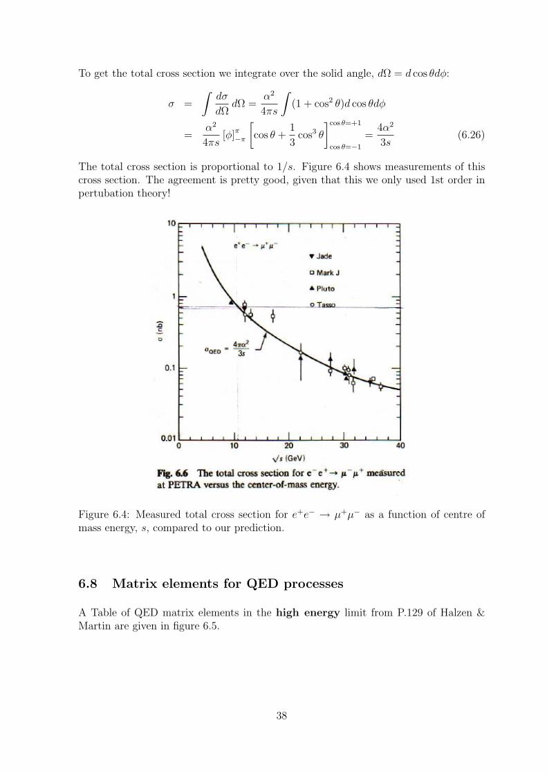
The total cross section is proportional to 1/s. Figure 6.4 shows measurements of thiscross section. The agreement is pretty good, given that this we only used 1st order inpertubation theory!

Figure 6.4: Measured total cross section for e+e− → µ

+µ− as a function of centre of

mass energy, s, compared to our prediction.

6.8 Matrix elements for QED processes

A Table of QED matrix elements in the high energy limit from P.129 of Halzen &Martin are given in figure 6.5.

38

Figure 6.5: QED matrix elements for lowest order processes in terms of the Mandelstamvariables.

39

µ−

e−

k

µ−

q − k

e−

e−

µ+

k

e+

µ−

q − k

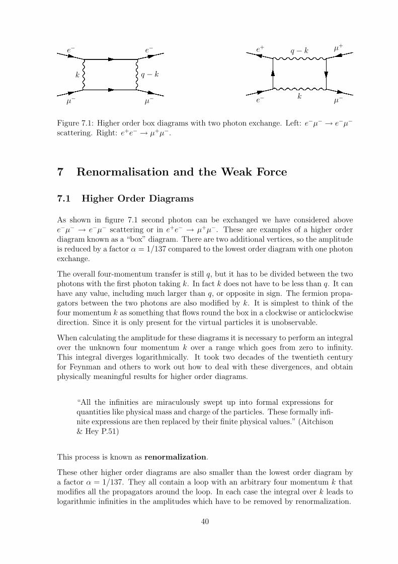
Figure 7.1: Higher order box diagrams with two photon exchange. Left: e−µ− → e

−µ−

scattering. Right: e+e− → µ

+µ−.

7 Renormalisation and the Weak Force

7.1 Higher Order Diagrams

As shown in figure 7.1 second photon can be exchanged we have considered abovee−µ− → e

−µ− scattering or in e

+e− → µ

+µ−. These are examples of a higher order

diagram known as a “box” diagram. There are two additional vertices, so the amplitudeis reduced by a factor α = 1/137 compared to the lowest order diagram with one photonexchange.

The overall four-momentum transfer is still q, but it has to be divided between the twophotons with the first photon taking k. In fact k does not have to be less than q. It canhave any value, including much larger than q, or opposite in sign. The fermion propa-gators between the two photons are also modified by k. It is simplest to think of thefour momentum k as something that flows round the box in a clockwise or anticlockwisedirection. Since it is only present for the virtual particles it is unobservable.

When calculating the amplitude for these diagrams it is necessary to perform an integralover the unknown four momentum k over a range which goes from zero to infinity.This integral diverges logarithmically. It took two decades of the twentieth centuryfor Feynman and others to work out how to deal with these divergences, and obtainphysically meaningful results for higher order diagrams.

“All the infinities are miraculously swept up into formal expressions forquantities like physical mass and charge of the particles. These formally infi-nite expressions are then replaced by their finite physical values.” (Aitchison& Hey P.51)

This process is known as renormalization.

These other higher order diagrams are also smaller than the lowest order diagram bya factor α = 1/137. They all contain a loop with an arbitrary four momentum k thatmodifies all the propagators around the loop. In each case the integral over k leads tologarithmic infinities in the amplitudes which have to be removed by renormalization.

40

e−

e−

e−

e−

e−

e−

Figure 7.2: Some other higher order diagrams. Top left: a “dressed fermion” emitsand reabsorbs a virtual photon. Top right: a “bubble” diagram where a virtual photoncreates and annihilates a fermion-antifermion pair. Bottom: a “vertex correction” wherea virtual photon connects two fermion lines across a vertex. The black blob representsan electromagnetic vertex which is not described in full.

7.2 Renormalization

In QED the divergent terms from higher order contributions to the amplitude areabsorbed into a redefinition of the charge e =

√4πα responsible for the vertex coupling,

and a redefinition of the fermion mass m which enters through fermion propagators:

eR = e0 + δe mR = m0 + δm (7.1)

The quantities e0 and m0 are known as the “bare” charge and mass. These wouldbe the physical values if there were no higher order diagrams. Since there are alwayshigher order diagrams, the bare values are unmeasurable. The remormalised physicalvalues eR and mR are the ones we measure: they include δe and δm corrections fromhigher order diagrams, even though these are infinite! Rather bizarrely there must becancellations between the infinities in δe, δm and the bare quantities e0, m0.

The renormalization process can be explicitly shown by imposing a “cutoff” mass M

on the integral over the loop four momentum k. The integral then gives a finite partindependent of M , and a part dependent on M which goes to infinity when the cutoffis removed (see Griffiths P. 219, P.264 and Halzen & Martin P. 157). The renormalizedcharge absorbs the infinite M dependent part (here we have just included electron-positron loops):

eR = e0

1−e20

12π2ln

M2

q2

(7.2)

Taking a finite scale for M leads to a variation of the physical charge e as a function ofthe four momentum transfer q

2. This “running coupling constant” is discussed in thenext section.

41

A way to understand renormalization is to say that the higher order contributions areabsorbed into re-definitions of the Feynman diagrams:

• A dressed fermion contribution can be absorbed into a re-definition of the spinor,modifying the fermion mass.

• A bubble diagram can be absorbed into a re-definition of the photon propaga-tor. This introduces lepton-antilepton and quark-antiquark components into thephoton!

• A vertex correction can be absorbed into a re-definition of the coupling charge atthe vertex. This can be thought of as being a result of charge screening due tofermion/antifermion pairs.

7.3 Running Coupling Constants

The finite parts of the higher order corrections lead to a q2 dependence of the vertex

couplings. Starting from the renormalized physical charge at q2 = 0 the “running”

coupling constant is:

α(q2) = α(0)

1 + α(0)

zf

3πln(

q2

M2)

(7.3)

where zf =

f Q2f is the sum over the charges of all the active fermion/antifermion

pairs (in units of e). zf has a dependence on q2 as more fermions become active. At

low q2 we can use zf = 1 (only e

+e− pairs), but at 100 GeV we need zf = 38/9 ≈ 4

(only tt pairs not active).

Since M is an arbitrary large cut-off mass, the above form is not particularly useful.What is usually done is to select a renormalization scale, q

2 = µ2, relative to which

α at any other value of q2 can be defined:

α(q2) = α(µ2)

1− α(µ2)

zf

3πln(

q2

µ2)

−1

(7.4)

We can choose any value of µ where make a initial measurement of α, but once wedo the evolution of the values of α are determined by equation (7.4). It is usual totake either a low energy reference from atomic physics (µ = 1 MeV) or a high energyreference from LEP (µ = mZ = 91 GeV )data:

α(µ = 0) =1

137α(µ2 = m

2Z) =

1

128(7.5)

Note that the running of the electromagnetic coupling α is quite small. We will seelater that this is not the case for the strong coupling αs.

7.4 Measurements of g − 2

Non-Examinable section - just included for your interest

42

The gyromagnetic ratio, g, for an electron, defines its magnetic moment, i.e. the couplingof its spin to a magnetic field:

µ = gµBS µB =

e2mec

(7.6)

where µB is the Bohr magneton. One of the successes of the Dirac equation is that itpredicts that g = 2 for “bare” fermions.

The lowest order Feynman diagram describing the magnetic moment couples the fermionto the electromagnetic field via a single virtual photon. The inclusion of higher orderdiagrams lead to an anomalous value for g slightly different from 2. QED has beenused to calculate diagrams up to O(α5), of which there are a very large number! Thetheoretical predictions for the electron and muon are:

g − 2

2

e

= 0.001159652183(8)

g − 2

2

µ

= 0.0011659183(5) (7.7)

where the numbers in brackets are the errors on the last digits. Note that the maintheoretical uncertainties are no longer associated with QED but with the introduction ofstrong interaction effects when a bubble diagram involves a quark-antiquark pair.

The experimental measurements of g − 2 use spin precession in a magnetic field. Theelectron is stable and can be held in a Penning trap to make the measurements. In thecase of the unstable muon, there has been a heroic series of experiments over the last50 years using storage rings. The current results are:

g − 2

2

e

= 0.0011596521807(3)

g − 2

2

µ

= 0.0011659209(6) (7.8)

These tests of QED are among the most accurate tests of a theory in the whole ofphysics. There is quite a lot of current interest in the (26 ± 8) × 10−10 differencebetween experiment and theory for the muon which has about 3σ significance. This maybe evidence for physics beyond the Standard Model giving rise to additional Feynmandiagrams. End of non-examinable section

7.5 Charged Currents

The W± bosons with mass MW = 80.4 GeV mediate weak charged current interactions:

• The heavy virtual W boson propagator is gµν

/(M2W − q

2).

• The current operator is purely left-handed γµ 1

2(1− γ5).

This is known as the V–A theory.

• The dimensionless coupling constant at each vertex, gW , is often written in termsof the dimensioned Fermi constant, GF = 1.16× 10−5GeV−2:

GF√

2=

g2W

8M2W

(7.9)

This comes from the low energy limit on the propagator q2 M

2W .

43

W−d

u

e−

νe

W+u

d

e+

νe

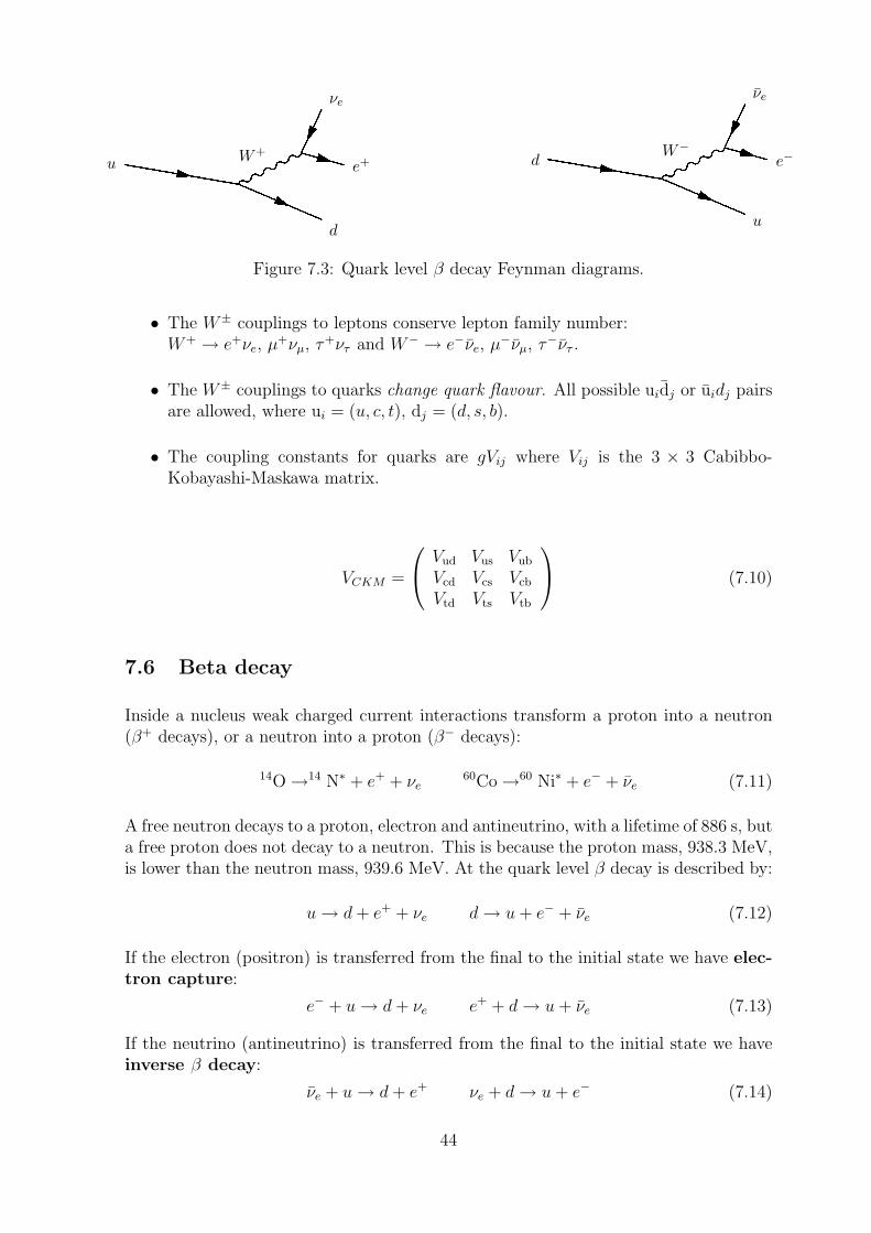
Figure 7.3: Quark level β decay Feynman diagrams.

• The W± couplings to leptons conserve lepton family number:

W+ → e

+νe, µ

+νµ, τ

+ντ and W

− → e−νe, µ

−νµ, τ

−ντ .

• The W± couplings to quarks change quark flavour. All possible uidj or uidj pairs

are allowed, where ui = (u, c, t), dj = (d, s, b).

• The coupling constants for quarks are gVij where Vij is the 3 × 3 Cabibbo-Kobayashi-Maskawa matrix.

VCKM =

Vud Vus Vub

Vcd Vcs Vcb

Vtd Vts Vtb

(7.10)

7.6 Beta decay

Inside a nucleus weak charged current interactions transform a proton into a neutron(β+ decays), or a neutron into a proton (β− decays):

14O→14 N∗ + e+ + νe

60Co→60 Ni∗ + e− + νe (7.11)

A free neutron decays to a proton, electron and antineutrino, with a lifetime of 886 s, buta free proton does not decay to a neutron. This is because the proton mass, 938.3 MeV,is lower than the neutron mass, 939.6 MeV. At the quark level β decay is described by:

u→ d + e+ + νe d→ u + e

− + νe (7.12)

If the electron (positron) is transferred from the final to the initial state we have elec-tron capture:

e− + u→ d + νe e

+ + d→ u + νe (7.13)

If the neutrino (antineutrino) is transferred from the final to the initial state we haveinverse β decay:

νe + u→ d + e+

νe + d→ u + e− (7.14)

44

7.6.1 Matrix element for β decay

The matrix element for β decay can be written in terms of quark and lepton currentscontaining the fermion spinors:

M =

g√

2udγ

µ 1

2(1− γ

5)uu

1

M2W − q2

g√

2uνeγ

µ 1

2(1− γ

5)ue

(7.15)

Hadronic interactions (form factors) play a role in decay rate and lifetimes, and theabove formula need to be modifed for these effects.

7.7 Muon decay

W−µ−(p1)

νµ(p3)

e(p4)

νe(p2)

gw

gw

The muon is a charged lepton that decays to an electron, a muon neutrino and anelectron antineutrino:

µ−→ e

−νµνe µ

+→ e

+νeνµ (7.16)

The matrix element can be written in terms of a muon-type current between the muonand the muon neutrino, and an electron-type current between the electron and theelectron antineutrino:

|M|2 =

g

2W

8m2W

2

[u(νµ)γµ(1− γ5)u(µ)]2[u(e)γµ(1− γ

5)v(νe)]2 (7.17)

Neglecting the masses of the electron and neutrinos the transition rate can be calculated(see Griffiths P.311-313):

dΓ

dEe=

G2F

4π3m

2µE

2e

1−

4Ee

3mµ

(7.18)

This is known as the Michel spectrum. Recent measurement of this are shown infigure 7.4. Near the endpoint E0 = mµ/2 the rate drops abruptly from a maximum tozero.

We can obtain the decay rate by integrating equation (7.18):

Γ =

mµ/2

0

dΓ

dEedEe =

G2F m

2µ

4π3

mµ/2

0

E2e

1−

4Ee

3m2µ

dEe (7.19)

As µ− → e

−νeνµ is the only possible decay, the lifetime of the muon is:

τ ≡1

Γ=

192π3

G2F m5

µ

=192π37

G2F m5

µc4

(7.20)

45

3

Momentum (MeV/c)15 20 25 30 35 40 45 50

p (M

eV/c

)!

-0.3

-0.2

-0.1

0

0.1

0.2 DataMonte Carlo

FIG. 2: (color online) Average momentum change of decaypositrons through the target and detector materials as a func-tion of momentum for data (closed circles) and Monte Carlo(open circles), measured as described in the text.

If ρ = ρH + ∆ρ and η = ηH + ∆η, then the angle-integrated muon decay spectrum can be written as:

N(x) = NS(x, ρH , ηH) + ∆ρN∆ρ(x) + ∆ηN∆η(x). (3)

This expansion is exact. It can also be generalized toinclude the angular dependence [2]. This is the basis forthe blind analysis. The measured momentum-angle spec-trum is fitted to the sum of a MC ‘standard’ spectrumNS produced with unknown Michel parameters ρH , ηH ,ξH , δH and additional ‘derivative’ MC distributions N∆ρ,N∆ξ, and N∆ξδ, with ∆ρ, ∆ξ, and ∆ξδ as the fitting pa-rameters. The hidden Michel parameters associated withNS are revealed only after all data analysis has been com-pleted. The fiducial region adopted for this analysis re-quires p < 50 MeV/c, |pz| > 13.7 MeV/c, pT < 38.5MeV/c, and 0.50 < | cos θ| < 0.84.

Fits over this momentum range including both ρ and ηcontain very strong correlations [3]. To optimize the pre-cision for ρ, η was fixed at the hidden value ηH through-out the blind analysis, then a refit was performed to shiftη to the accepted value. We find that ρ depends linearlyon the assumed value of η, with dρ/dη = 0.018.

Figure 3(a) shows the momentum spectrum from set Bin the angular range 0.70 < | cos θ| < 0.84. The probabil-ity for reconstructing muon decays is very high, as shownin Figs. 3(b) and (d). Thus, higher momentum decaysthat undergo hard interactions and are reconstructed atlower momenta can lead to an apparent reconstructionprobability above unity. Figures 3(c) and (e) show theresiduals of the fit of the decay spectrum from set B.Similar fits have been performed to the other data sets,yielding the results shown in Table I. The fit results for δare not adopted due to a problem with the polarization-dependent radiative corrections in the event generator[2], but are consistent with the separate analysis reportedin [2]. Fits to the angle-integrated spectra, which are in-dependent of δ, give nearly identical results for ρ.

The 11 additional data sets have been combined withfurther MC simulations to estimate the systematic un-certainties shown in Tables I and II. The largest effects

0 10 20 30 40 50

Yiel

d (E

vent

s)

0

500

1000

1500

2000210"

All eventsIn fiducial

| < 0.84#0.70 < |cos (a)Pr

obab

ility

0.99

0.995

1

1.005| < 0.84#0.7 < |cos (b)0

$(D

ata

- Fit)

/

-2

0

2| < 0.84#0.7 < |cos (c)

Prob

abili

ty

0.99

0.995

1

1.005| < 0.7#0.5 < |cos (d)

Momentum (MeV/c)0 10 20 30 40 50

$(D

ata

- Fit)

/

-2

0

2| < 0.7#0.5 < |cos (e)

FIG. 3: (color online) Panel (a) shows the muon decay spec-trum (solid curve) from surface muon set B vs. momentum,for events within 0.70 < | cos θ| < 0.84, as well as the eventswithin this angular region that pass the fiducial constraints(dot-dashed curve). The spectrum within 0.5 < | cos θ| < 0.7is similar. Panels (b) and (d) show the probability for recon-structing decays for the two angular ranges, as calculated bythe Monte Carlo. Panels (c) and (e) show the residuals forthe same angular ranges from the fit of set B to the MonteCarlo ‘standard’ spectrum plus derivatives.

arise from time-variations of the cathode foil locations [9]and the density of the DME gas, which change the driftvelocities and influence the DC efficiencies far from thesense wires. These parameters were monitored through-out the data taking, but only average values were used inthe analysis. Special data sets and MC simulations that

Figure 7.4: TWIST experiment at TRIMF in Canada measures µ+ → e

+νeνµ decay

spectrum. Excellent agreement between data and prediction!

46

Measurements of muon lifetime and mass used to define a value for GF (values fromPDG 2010)

τ = (2.19703± 0.00002)× 106 s m = 105.658367± 0.000004MeV (7.21)

Applying small corrections for finite electron mass and second order effects GF =1.166364(5)× 10−5 GeV

−2

We can compare the couplings in muon decay and superallowed β decay:

GF (µ) = 1.166× 10−5 GeV−2GF (β)|Vud| = (1.136± 0.003)× 10−5 GeV−2

These give the same value for GF with |Vud| ≈ 0.97.

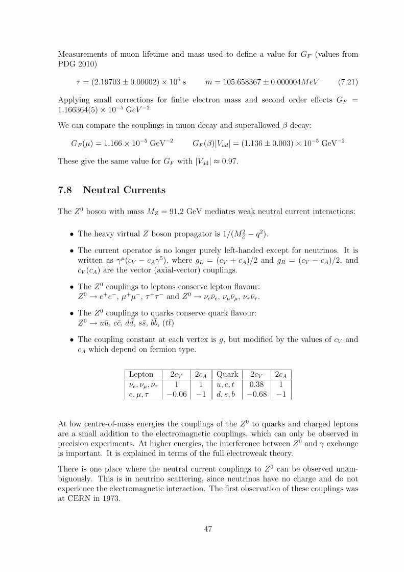
7.8 Neutral Currents

The Z0 boson with mass MZ = 91.2 GeV mediates weak neutral current interactions:

• The heavy virtual Z boson propagator is 1/(M2Z − q

2).

• The current operator is no longer purely left-handed except for neutrinos. It iswritten as γ

µ(cV − cAγ5), where gL = (cV + cA)/2 and gR = (cV − cA)/2, and

cV (cA) are the vector (axial-vector) couplings.

• The Z0 couplings to leptons conserve lepton flavour:

Z0 → e

+e−, µ

+µ−, τ

+τ− and Z

0 → νeνe, νµνµ, ντ ντ .

• The Z0 couplings to quarks conserve quark flavour:

Z0 → uu, cc, dd, ss, bb, (tt)

• The coupling constant at each vertex is g, but modified by the values of cV andcA which depend on fermion type.

Lepton 2cV 2cA Quark 2cV 2cA

νe, νµ, ντ 1 1 u, c, t 0.38 1e, µ, τ −0.06 −1 d, s, b −0.68 −1

At low centre-of-mass energies the couplings of the Z0 to quarks and charged leptons

are a small addition to the electromagnetic couplings, which can only be observed inprecision experiments. At higher energies, the interference between Z

0 and γ exchangeis important. It is explained in terms of the full electroweak theory.

There is one place where the neutral current couplings to Z0 can be observed unam-

biguously. This is in neutrino scattering, since neutrinos have no charge and do notexperience the electromagnetic interaction. The first observation of these couplings wasat CERN in 1973.

47