Quantization of the Free Dirac Field - University Of...
21
7 Quantization of the Free Dirac Field 7.1 The Dirac Equation and Quantum Field Theory The Dirac equation is a relativistic wave equation that describes the quan- tum dynamics of spinors. We will see in this section that a consistent de- scription of this theory cannot be done outside the framework of (local) relativistic Quantum Field Theory. The Dirac Equation (i/ ∂ - m)ψ =0 ¯ ψ(i/ ∂ + m)=0 (7.1) can be regarded as the equations of motion of a complex field ψ. Much as in the case of the scalar field, and also in close analogy to the theory of non- relativistic many particle systems discussed in the last chapter, the Dirac field is an operator which acts on a Fock space. We have already discussed that the Dirac equation also follows from a least-action-principle. Indeed the Lagrangian L = i 2 [ ¯ ψ/ ∂ψ - (∂ μ ¯ ψ)γ μ ψ] - m ¯ ψψ ≡ ¯ ψ(i/ ∂ - m)ψ (7.2) has the Dirac equation for its equation of motion. Also, the momentum Π α (x) canonically conjugate to ψ α (x) is Π ψ α (x)= δL δ∂ 0 ψ α (x) = iψ † α (7.3) Thus, they obey the equal-time Poisson Brackets {ψ α (x), Π ψ β (y)} PB = iδ αβ δ 3 (x - y) (7.4) Thus {ψ α (x), ψ † β (y)} PB = δ αβ δ 3 (x - y) (7.5)
Transcript of Quantization of the Free Dirac Field - University Of...
7
Quantization of the Free Dirac Field
7.1 The Dirac Equation and Quantum Field Theory
The Dirac equation is a relativistic wave equation that describes the quan-tum dynamics of spinors. We will see in this section that a consistent de-scription of this theory cannot be done outside the framework of (local)relativistic Quantum Field Theory.
The Dirac Equation
(i/! !m)" = 0 "(i/! +m) = 0 (7.1)
can be regarded as the equations of motion of a complex field ". Much as inthe case of the scalar field, and also in close analogy to the theory of non-relativistic many particle systems discussed in the last chapter, the Diracfield is an operator which acts on a Fock space. We have already discussedthat the Dirac equation also follows from a least-action-principle. Indeed theLagrangian
L =i
2["/!" ! (!µ")#
µ"]!m"" " "(i/! !m)" (7.2)
has the Dirac equation for its equation of motion. Also, the momentum!!(x) canonically conjugate to "!(x) is
!"!(x) =$L
$!0"!(x)= i"†
! (7.3)
Thus, they obey the equal-time Poisson Brackets
{"!(x),!"# (y)}PB = i$!#$3(x! y) (7.4)
Thus
{"!(x),"†#(y)}PB = $!#$
3(x! y) (7.5)
198 Quantization of the Free Dirac Field
In other words the field "! and its adjoint "†! are a canonical pair. This
result follows from the fact that the Dirac Lagrangian is first order in timederivatives. Notice that the field theory of non-relativistic many-particlesystems (for both fermions on bosons) also has a Lagrangian which is firstorder in time derivatives. We will see that, because of this property, thequantum field theory of both types of systems follows rather similar lines,at least at a formal level. As in the case of the many-particle systems, twotypes of statistics are available to us: Fermi and Bose. We will see that onlythe choice of Fermi statistics leads to a physically meaningful theory of theDirac equation.
The Hamiltonian for the Dirac theory is
H =
!d3x "!(x)
"! i! ·!+m
#
!#"#(x) (7.6)
where the fields "(x) and " = "†#0 are operators which act on a Hilbertspace to be specified below. Notice that the one-particle operator in Eq. (7.6)is just the one-particle Dirac Hamiltonian obtained if we regard the DiracEquation as a Schrodinger Equation for spinors. We will leave the issue oftheir commutation relations (i.e., Fermi or Bose) open for the time being.In any event, the equations of motion are independent of that choice (i.e.,do not depend on the statistics).
In the Heisenberg representation, we find
i#0!0" ="#0",H
#= (!i! ·!+m)" (7.7)
which is just the Dirac equation.We will solve these equations by means of a Fourier expansion in modes
of the form
"(x) =
!d3p
(2%)3m
&(p)
$"+(p)e
!ip·x + "!(p)eip·x%
(7.8)
where &(p) is a quantity with units of energy, and which will turn out to beequal to p0 =
&p2 +m2, and p · x = p0x0 ! p · x. In terms of "±(p), the
Dirac equation becomes
(p0#0 ! ! · p±m) "±(p) = 0 (7.9)
In other words, "±(p) creates one-particle states with energy ±p0. Let usmake the substitution
"±(p) = (±/p+m)' (7.10)
7.1 The Dirac Equation and Quantum Field Theory 199
We get
(/p#m)(±/p+m)' = ±(p2 !m2)' = 0 (7.11)
This equation has non-trivial solutions only if the mass-shell condition isobeyed
p2 !m2 = 0 (7.12)
Thus, we can identify p0 = &(p) =&(p2 +m2. At zero momentum these
states become
"±(p0,p = 0) = (±p0#0 +m)' (7.13)
where ' is an arbitrary 4-spinor. Let us choose ' to be an eigenstate of #0.Recall that in the Dirac representation #0 is diagonal
#0 =
'I 00 !I
((7.14)
Thus the spinors u(1)(m,0) and u(2)(m,0)
u(1)(m,0) =
)
**+
1000
,
--. u(2)(m,0) =
)
**+
0100
,
--. (7.15)
have #0-eigenvalue +1
#0u(i)(m,0) = +u($)(m,0) ) = 1, 2 (7.16)
and the spinors v($)(m,0)() = 1, 2)
v(1)(m,0) =
)
**+
0010
,
--. v(2)(m,0) =
)
**+
0001
,
--. (7.17)
have #0-eigenvalue !1,
#0v($)(m,0) = !v($)(m,0) ) = 1, 2 (7.18)
Let *(i)(m, 0) be the 2-spinors () = 1, 2)
*(1) =
'10
(*(2) =
'01
((7.19)
200 Quantization of the Free Dirac Field
In terms of *(i) the solutions are
"+(p) = u($)(p) =(/p+m)&2m(p0 +m)
u($)(m,0) =
)
+
/p0+m2m *($)(m, 0)
!·p$2m(p0+m)
*($)(m, 0)
,
.
(7.20)and
"!(p) = v($)(p) =(!/p+m)&2m(p0 +m)
v($)(m,0) =
)
+!·p$
2m(p0+m)*($)(m,0)
/p0+m2m *($)(m,0)
,
.
(7.21)where the two solutions "+(p) have energy +p0 = +
&p2 +m2 while "!(p)
have energy !p0 = !&p2 +m2.
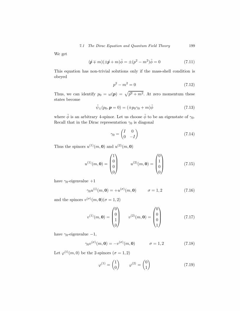
Therefore, the one-particle states of the Dirac theory can have both posi-tive and negative energy and, as it stands, the spectrum of the one-particleDirac Hamiltonian, shown schematically in Fig. 10.15, is not positive. Inaddition, each Dirac state has a two-fold degeneracy due to the spin of theparticle.
E
|p|
m
!m
Figure 7.1 Single particle specrum of the Dirac theory.
The spinors u(i) and v(i) have the normalization
u($)(p)u(%)(p) = $$%
v($)(p)v(%)(p) = !$$%u($)(p)v(%)(p) = 0
(7.22)
7.1 The Dirac Equation and Quantum Field Theory 201
where u = u†#0 and v = v†#0. It is straightforward to check that the opera-tors "±(p)
"±(p) =1
2m(±/p+m) (7.23)
are projection operators that project the spinors onto the subspaces withpositive ("+) and negative ("!) energy respectively. These operators satisfy
"2± = "± Tr "± = 2 "+ + "! = 1 (7.24)
Hence, the four 4-spinors u($) and v($) are orthonormal and complete, andprovide a natural basis of the Hilbert space of single-particle states.
We can use these results to write the expansion of the field operator
"(x) =
!d3p
(2%)3m
p0
0
$=1,2
"a$,+(p)u
($)+ (p)e!ip·x+a$,!(p)v
($)! (p)eip·x
#(7.25)
where the coe#cients a$,±(p) are operators with as yet unspecified commu-tation relations. The (formal) Hamiltonian for this system is
H =
!d3p
(2%)3m
p0
0
$=1,2
p0[a†$,+(p)a$,+(p)! a†$,!(p)a$,!(p)] (7.26)
Since the single-particle spectrum does not have a lower bound, any attemptto quantize the theory with canonical commutation relations will have theproblem that the total energy of the system is not bounded from below. Inother words “Dirac bosons” do not have a ground state and the systemis unstable since we can put as many bosons as we wish in states witharbitrarily large but negative energy.
Dirac realized that the simple and elegant way out of this problem wasto require the electrons to obey the Pauli Exclusion Principle since, in thatcase, there is a natural and stable ground state. However, this assumptionimplies that the Dirac theory must be quantized as a theory of fermions.Hence we are led to quantize the theory with canonical anticommutationrelations
{as,$(p), as!,$!(p")} = 0
{as,$(p), a†s!,$!(p")} = (2%)3
p0m$3(p! p")$ss!$$$!
(7.27)
where s = ±. Let us denote by |0% the state anihilated by the operatorsas,$(p),
as,$(p)|0% = 0 (7.28)
202 Quantization of the Free Dirac Field
We will see now that this state is not the vacuum (or ground state) of theDirac theory. Let us now discuss the construction of the ground state andof the excitation spectrum.
7.1.1 Ground State and Normal Ordering
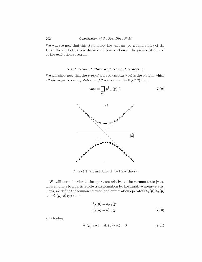
We will show now that the ground state or vacuum |vac% is the state in whichall the negative energy states are filled (as shown in Fig.7.2) i.e.,
|vac% =1
$,p
a†!,$(p)|0% (7.29)
E
|p|
Figure 7.2 Ground State of the Dirac theory.
We will normal-order all the operators relative to the vacuum state |vac%.This amounts to a particle-hole transformation for the negative energy states.Thus, we define the fermion creation and annihilation operators b$(p), b
†$(p)
and d$(p), d†$(p) to be
b$(p) = a$,+(p)
d$(p) = a†$,!(p) (7.30)
which obey
b$(p)|vac% = d$(p)|vac% = 0 (7.31)
7.1 The Dirac Equation and Quantum Field Theory 203
E
|p|
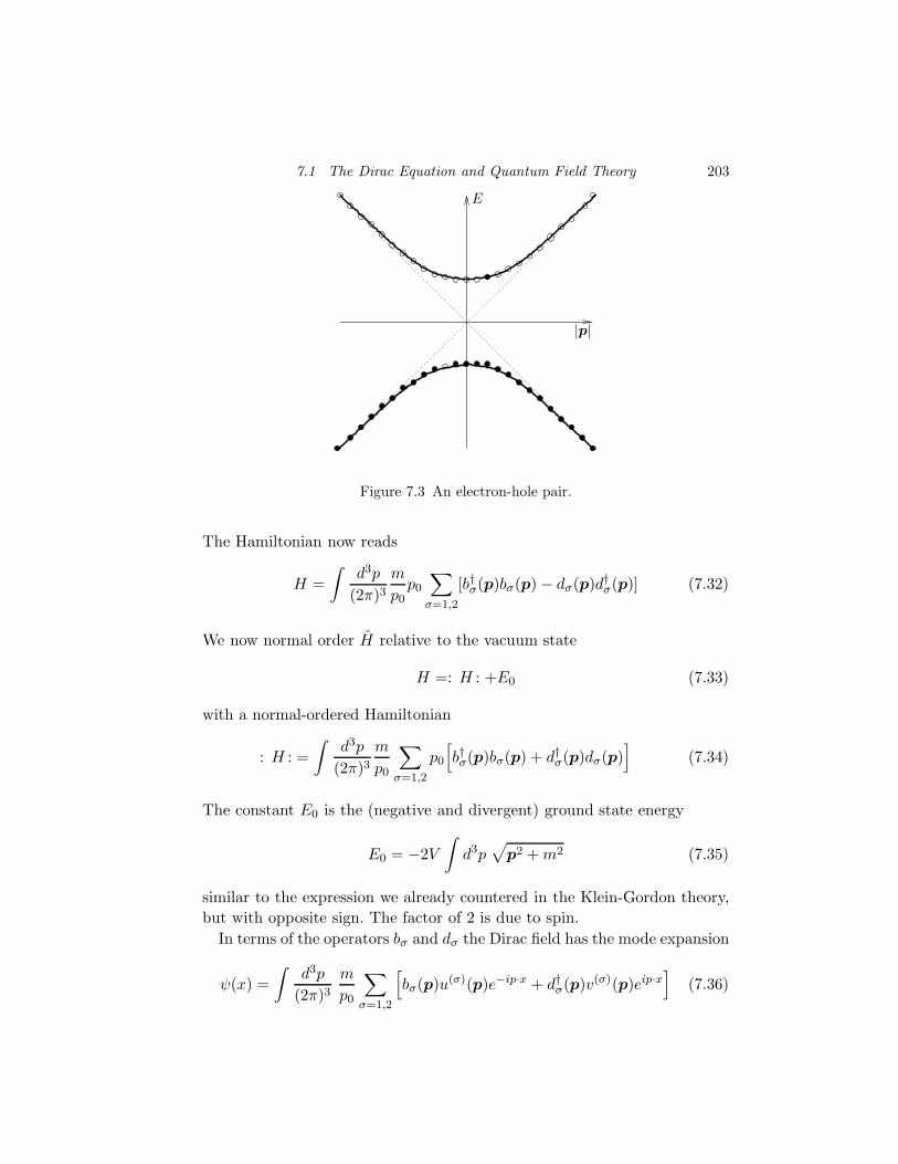
Figure 7.3 An electron-hole pair.
The Hamiltonian now reads
H =
!d3p
(2%)3m
p0p00
$=1,2
[b†$(p)b$(p)! d$(p)d†$(p)] (7.32)
We now normal order H relative to the vacuum state
H =: H : +E0 (7.33)
with a normal-ordered Hamiltonian
: H : =
!d3p
(2%)3m
p0
0
$=1,2
p0"b†$(p)b$(p) + d†$(p)d$(p)
#(7.34)
The constant E0 is the (negative and divergent) ground state energy
E0 = !2V!
d3p&
p2 +m2 (7.35)
similar to the expression we already countered in the Klein-Gordon theory,but with opposite sign. The factor of 2 is due to spin.
In terms of the operators b$ and d$ the Dirac field has the mode expansion
"(x) =
!d3p
(2%)3m
p0
0
$=1,2
"b$(p)u
($)(p)e!ip·x + d†$(p)v($)(p)eip·x
#(7.36)
204 Quantization of the Free Dirac Field
which satisfy equal-time canonical anticommutation relations
{"(x),"†(x")} = $3(x! x")
{"(x),"(x")} = {"†(x),"†(x")} = 0 (7.37)
7.1.2 One-particle states
The excitations of this theory can be constructed by using the same methodsemployed for non-relativistic many-particle systems. Let us first constructthe total four-momentum operator Pµ
Pµ =
!d3x T 0µ =
!d3p
(2%)3m
p0pµ0
$=1,2
: b†$(p)b$(p)! d$(p)d†$(p) : (7.38)
Hence
: Pµ :=
!d3p
(2%)3m
p0pµ0
$=1,2
"b†$(p)b$(p) + d†$(p)d$(p)
#(7.39)
The states b†$(p)|vac% and d†$(p)|vac% have energy p0 =&p2 +m2 and mo-
mentum p, i.e.,
: H : b†$(p)|vac% =p0b†$(p)|vac%
: H : d†$(p)|vac% =p0d†$(p)|vac%
: P i : b†$(p)|vac% =pib†$(p)|vac%: P i : d†$(p)|vac% =pid†$(p)|vac% (7.40)
We see that there are four di$erent states which have the same energy andmomentum. Let us find quantum numbers to classify these states.
7.1.3 Spin
The angular momentum tensor Mµ%& for the Dirac theory is
Mµ%& =
!d3x i"(x) #µ(x%!& ! x&!% + %%&) "(x) (7.41)
where %%& is the matrix
%%& =1
2)%& =
1
4[#% , #&] (7.42)
The conserved angular momentum J%& is
J%& = M0%& =
!d3x i"†(x)(x%!& ! x&!% + %%&) "(x) (7.43)
7.1 The Dirac Equation and Quantum Field Theory 205
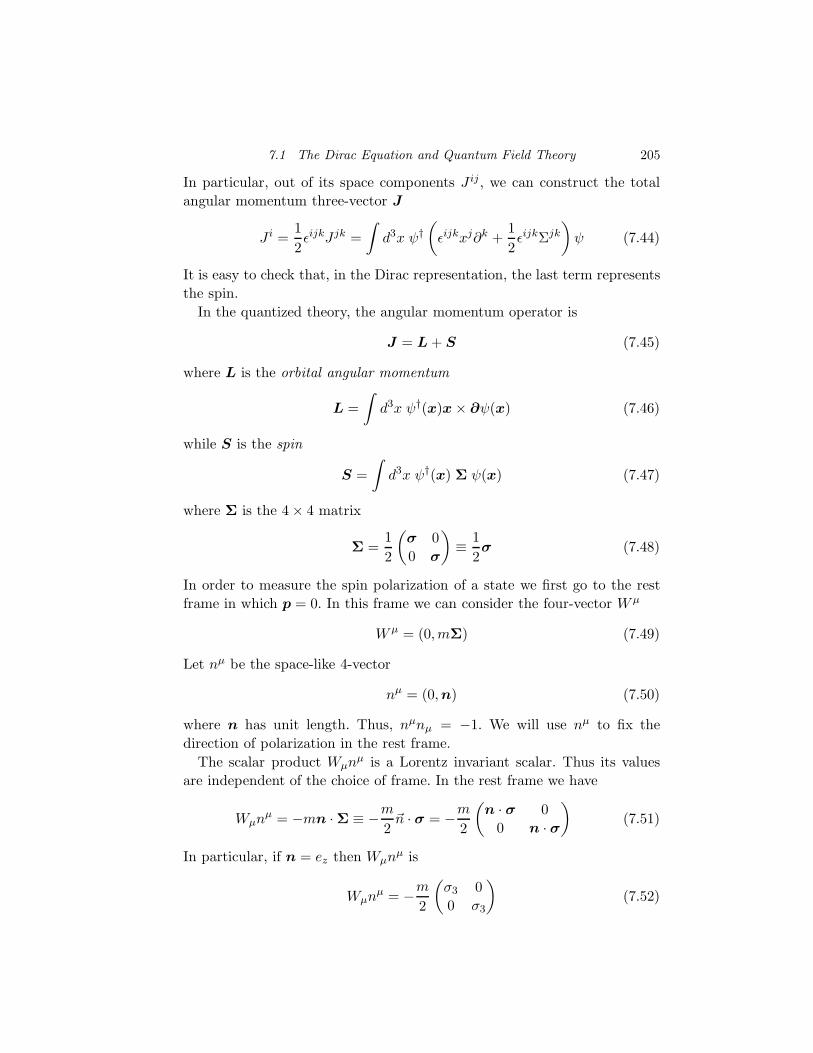
In particular, out of its space components J ij , we can construct the totalangular momentum three-vector J
J i =1
2+ijkJ jk =
!d3x "†
'+ijkxj!k +
1
2+ijk%jk
(" (7.44)
It is easy to check that, in the Dirac representation, the last term representsthe spin.
In the quantized theory, the angular momentum operator is
J = L+ S (7.45)
where L is the orbital angular momentum
L =
!d3x "†(x)x& ""(x) (7.46)
while S is the spin
S =
!d3x "†(x) ! "(x) (7.47)
where ! is the 4& 4 matrix
! =1
2
'# 00 #
(" 1
2# (7.48)
In order to measure the spin polarization of a state we first go to the restframe in which p = 0. In this frame we can consider the four-vector W µ
W µ = (0,m!) (7.49)
Let nµ be the space-like 4-vector
nµ = (0,n) (7.50)
where n has unit length. Thus, nµnµ = !1. We will use nµ to fix thedirection of polarization in the rest frame.
The scalar product Wµnµ is a Lorentz invariant scalar. Thus its valuesare independent of the choice of frame. In the rest frame we have
Wµnµ = !mn ·! " !m
2(n · # = !m
2
'n · # 00 n · #
((7.51)
In particular, if n = ez then Wµnµ is
Wµnµ = !m
2
')3 00 )3
((7.52)
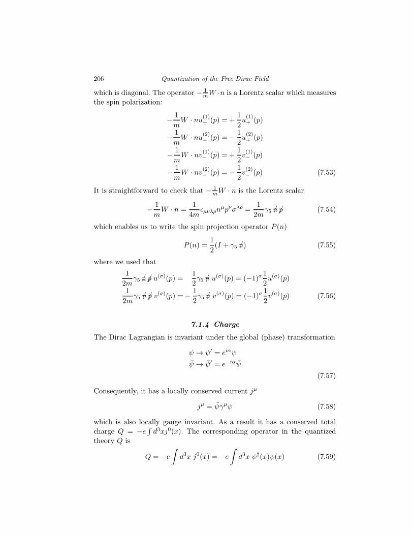
206 Quantization of the Free Dirac Field
which is diagonal. The operator ! 1mW ·n is a Lorentz scalar which measures
the spin polarization:
! 1
mW · nu(1)+ (p) = +
1
2u(1)+ (p)
! 1
mW · nu(2)+ (p) =! 1
2u(2)+ (p)
! 1
mW · nv(1)! (p) = +
1
2v(1)! (p)
! 1
mW · nv(2)! (p) =! 1
2v(2)! (p) (7.53)
It is straightforward to check that ! 1mW · n is the Lorentz scalar
! 1
mW · n =
1
4m+µ%&'n
µp%)&' =1
2m#5 /n /p (7.54)
which enables us to write the spin projection operator P (n)
P (n) =1
2(I + #5 /n) (7.55)
where we used that
1
2m#5 /n /p u($)(p) =
1
2#5 /n u($)(p) = (!1)$ 1
2u($)(p)
1
2m#5 /n /p v($)(p) =! 1
2#5 /n v($)(p) = (!1)$ 1
2v($)(p) (7.56)
7.1.4 Charge
The Dirac Lagrangian is invariant under the global (phase) transformation
" ' "" = ei!"
" ' "" = e!i!"
(7.57)
Consequently, it has a locally conserved current jµ
jµ = "#µ" (7.58)
which is also locally gauge invariant. As a result it has a conserved totalcharge Q = !e
2d3xj0(x). The corresponding operator in the quantized
theory Q is
Q = !e!
d3x j0(x) = !e!
d3x "†(x)"(x) (7.59)
7.1 The Dirac Equation and Quantum Field Theory 207
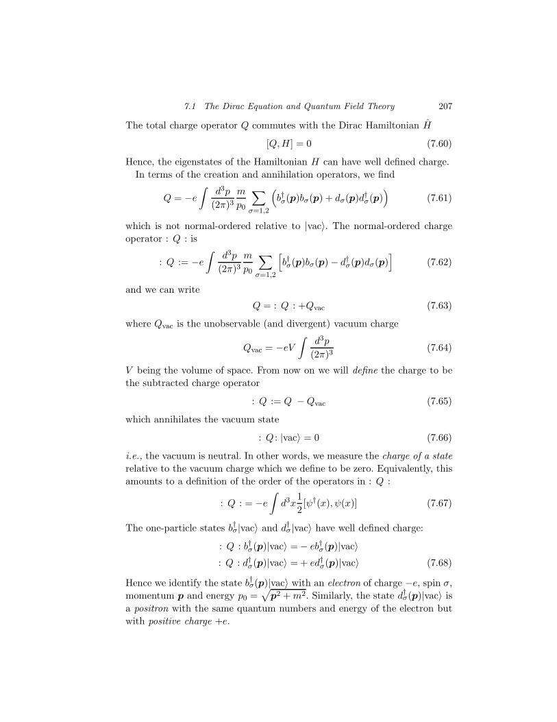
The total charge operator Q commutes with the Dirac Hamiltonian H
[Q,H] = 0 (7.60)
Hence, the eigenstates of the Hamiltonian H can have well defined charge.In terms of the creation and annihilation operators, we find
Q = !e!
d3p
(2%)3m
p0
0
$=1,2
$b†$(p)b$(p) + d$(p)d
†$(p)
%(7.61)
which is not normal-ordered relative to |vac%. The normal-ordered chargeoperator : Q : is
: Q := !e!
d3p
(2%)3m
p0
0
$=1,2
"b†$(p)b$(p)! d†$(p)d$(p)
#(7.62)
and we can write
Q = : Q : +Qvac (7.63)
where Qvac is the unobservable (and divergent) vacuum charge
Qvac = !eV!
d3p
(2%)3(7.64)
V being the volume of space. From now on we will define the charge to bethe subtracted charge operator
: Q := Q !Qvac (7.65)
which annihilates the vacuum state
: Q : |vac% = 0 (7.66)
i.e., the vacuum is neutral. In other words, we measure the charge of a staterelative to the vacuum charge which we define to be zero. Equivalently, thisamounts to a definition of the order of the operators in : Q :
: Q : = !e!
d3x1
2["†(x),"(x)] (7.67)
The one-particle states b†$|vac% and d†$|vac% have well defined charge:
: Q : b†$(p)|vac% =! eb†$(p)|vac%: Q : d†$(p)|vac% =+ ed†$(p)|vac% (7.68)
Hence we identify the state b†$(p)|vac% with an electron of charge !e, spin ),momentum p and energy p0 =
&p2 +m2. Similarly, the state d†$(p)|vac% is
a positron with the same quantum numbers and energy of the electron butwith positive charge +e.
208 Quantization of the Free Dirac Field
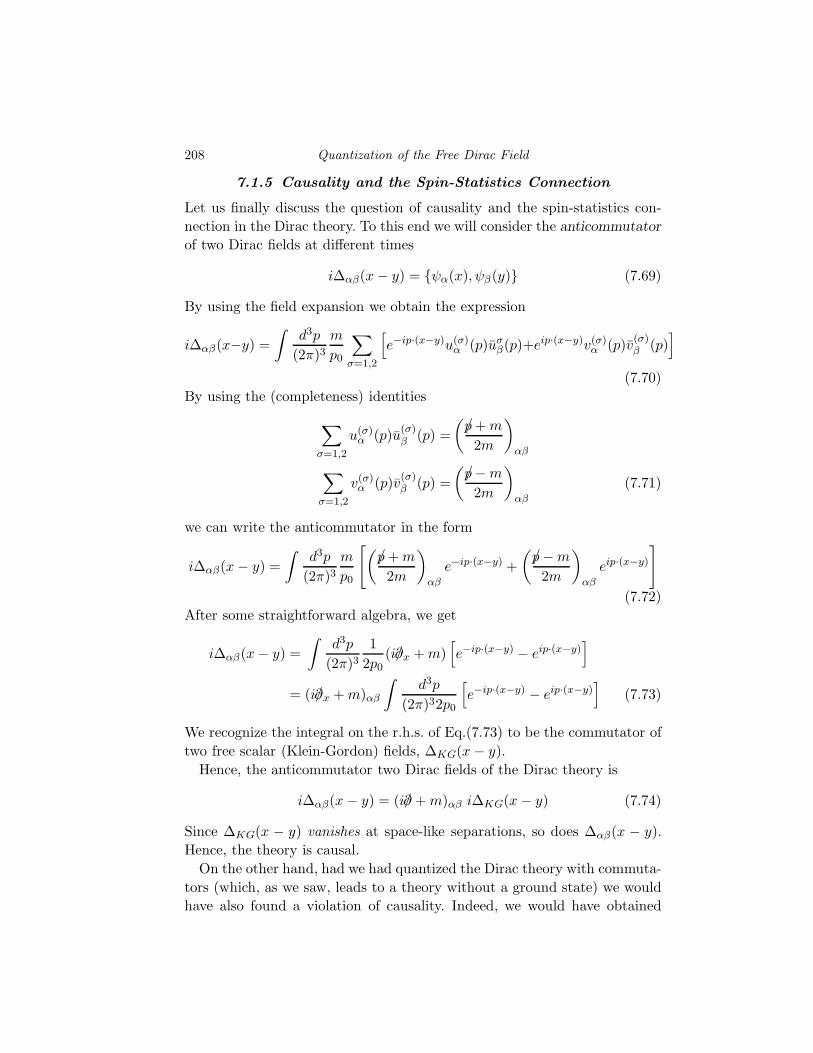
7.1.5 Causality and the Spin-Statistics Connection
Let us finally discuss the question of causality and the spin-statistics con-nection in the Dirac theory. To this end we will consider the anticommutator
of two Dirac fields at di$erent times
i&!#(x! y) = {"!(x),"#(y)} (7.69)
By using the field expansion we obtain the expression
i&!#(x!y) =!
d3p
(2%)3m
p0
0
$=1,2
"e!ip·(x!y)u($)! (p)u$#(p)+eip·(x!y)v($)! (p)v($)# (p)
#
(7.70)By using the (completeness) identities
0
$=1,2
u($)! (p)u($)# (p) =
'/p+m
2m
(
!#
0
$=1,2
v($)! (p)v($)# (p) =
'/p!m
2m
(
!#
(7.71)
we can write the anticommutator in the form
i&!#(x! y) =
!d3p
(2%)3m
p0
3'/p+m
2m
(
!#
e!ip·(x!y) +
'/p!m
2m
(
!#
eip·(x!y)
4
(7.72)After some straightforward algebra, we get
i&!#(x! y) =
!d3p
(2%)31
2p0(i/!x +m)
"e!ip·(x!y) ! eip·(x!y)
#
= (i/!x +m)!#
!d3p
(2%)32p0
"e!ip·(x!y) ! eip·(x!y)
#(7.73)
We recognize the integral on the r.h.s. of Eq.(7.73) to be the commutator oftwo free scalar (Klein-Gordon) fields, &KG(x! y).
Hence, the anticommutator two Dirac fields of the Dirac theory is
i&!#(x! y) = (i/! +m)!# i&KG(x! y) (7.74)
Since &KG(x ! y) vanishes at space-like separations, so does &!#(x ! y).Hence, the theory is causal.
On the other hand, had we had quantized the Dirac theory with commuta-tors (which, as we saw, leads to a theory without a ground state) we wouldhave also found a violation of causality. Indeed, we would have obtained

7.1 The Dirac Equation and Quantum Field Theory 209
instead the result
&!#(x! y) = (i/! +m)!#&(x! y) (7.75)
where &(x! y) is given by
&(x! y) =
!d3p
(2%)32p0
$e!ip·(x!y) + eip·(x!y)
%(7.76)
which does not vanish at space-like separations. Instead, at equal times andat long distances 5&(x! y) decays as
&(R, 0) ( e!MR
R2MR') (7.77)
Thus, if the Dirac theory were to be quantized with commutators, the fieldoperators would not commute at equal times at distances shorter than theCompton wavelength. This would be a violation of locality. The same resultholds in the theory of the scalar field if it is quantized with anticommutators.
These results can be summarized in the Spin-Statistics Theorem: fieldswith half-integer spin must be quantized as fermions, i.e. obey canonicalanti-commutation relations, whereas fields with integer spin must be quan-tized as bosons, i.e. obey canonical commutation relations. If a field theoryis quantized with the wrong spin-statistics connection, either the theorybecomes non-local, with violations of causality, and/or it does not have aground state, or it contains states in its spectrum with negative norm. No-tice that the arguments we have used were derived for free local theories. Itis a highly non-trivial task to prove that the spin-statistics connection alsoremains valid for interacting theories. Although this can be done by makingsu#ciently strong assumptions of the behavior of perturbation theory, inreality it must the spin-statistics connection must be regarded as an axiomof local relativistic quantum field theories.
7.1.6 The Propagator of the spinor field
Finally, we will compute the propagator for a spinor field "!(x). We will findthat it is essentially the Green function for the the Dirac operator i/! !m.The propagator is defined by
S!#(x! x") = !i*vac|T"!(x)"#(x")|vac% (7.78)
where we have used the time ordered product of two fermionic field opera-tors, which is defined by
T"!(x)"#(x") = ,(x0 ! x"0)"!(x)"#(x
")! ,(x"0 ! x0)"#(x")"!(x) (7.79)
210 Quantization of the Free Dirac Field
Notice the change in sign with respect to the time ordered product of bosonicoperators. The sign change reflects the anticommutation properties of thefield.
We will show now that this propagator is closely connected to the propa-gator of the free scalar field, i.e., the Green function for the Klein-Gordonoperator !2 +m2.
By acting with the Dirac operator on S!#(x! x") we find6i/! !m
7!#
S#&(x! x") = !i6i/! !m
7!#*vac|T"#(x)"&(x")|vac% (7.80)
We now use that!
!x0,(x0 ! x"0) = $(x0 ! x"0) (7.81)
and the fact that the equation of motion of the Heisenberg field operators"! is the Dirac equation,
6i/! !m
7!#"#(x) = 0 (7.82)
to show that$i/! !m
%
!#S#&(x! x") =
!i*vac|T6i/! !m
7!#"#(x)"&(x
")|vac%
+$(x0 ! x"0)$*vac|#0!#"#(x)"&(x")|vac%
+*vac|"&(x")#0!#"#(x)|vac%%
=$(x0 ! x"0)#0!#*vac|
8"#(x),"
†%(x
")9|vac%#0%&
=$(x0 ! x"0)$3(x! x")$!& (7.83)
Therefore we find that S#&(x! x") is the solution of the equation6i/! !m
7!#
S#&(x! x") = $4(x! x")$!& (7.84)
Hence S#&(x! x") = !i*vac|T"#(x)"&(x")|vac% is the Green function of theDirac operator.
We saw before that there is a close connection between the Dirac andthe Klein-Gordon operators. We will now use this connection to relate theirpropagators. Let us write the Green function S!&(x! x") in the form
S!&(x! x") =6i/! +m
7!#
G#&(x! x") (7.85)
Since S!&(x! x") satisfies Eq.(7.84), we find that6i/! !m
7!#
S#&(x! x") =6i/! !m
7!#
6i/! +m
7#%
G%&(x! x") (7.86)
7.2 Discrete Symmetries of the Dirac Theory 211
But6i/! !m
7!#
6i/! +m
7#%
= !6!2 +m2
7$!% (7.87)
Hence, G!%(x! x") must satisfy
!6!2 +m2
7G!%(x! x") = $4(x! x")$!% (7.88)
Therefore G!%(x! x") is given by
G!%(x! x") = G(x! x")$!% (7.89)
where G(x!x") is the propagator for a scalar field, i.e., the Green functionof the Klein-Gordon equation
!6!2 +m2
7G(x! x") = $4(x! x") (7.90)
We then conclude that the Dirac propagator S!#(x ! x"), and the Klein-Gordon propagator G(x! x") are related by
S!#(x! x") =6i/! +m
7!#
G(x! x") (7.91)
In particular, this relationship implies that the have exactly the same asymp-totic behaviors that we discussed before. The spinor structure of the Diracpropagator is determined by the operator in front of G(x! x") in Eq.(7.91).
The Feynman propagator for the Dirac field, given by Eq. (7.91), in mo-mentum space becomes
S!#(p) =
'/p+m
p2 !m2 + i+
(
!#
(7.92)
Hence we get the same pole structure in the time-ordered propagator as wedid for the Klein-Gordon field.
7.2 Discrete Symmetries of the Dirac Theory
We will now discuss three important discrete symmetries in relativistic fieldtheories: charge conjugation, parity and time reversal. These discrete sym-metries have a di$erent role, and a di$erent standing, than the continu-ous symmetries discussed before. In a relativistic quantum field theory theground state, i.e., the vacuum, must be invariant under continuous Lorentztransformations, but it may not be invariant under C, P or T . However, ina local relativistic quantum field theory the product CPT is always a goodsymmetry. This is in fact an axiom of relativistic local quantum field theory.Thus, although C, P or T may or may not to be good symmetries of the

212 Quantization of the Free Dirac Field
vacuum state, CPT must be a good symmetry. As in the case of the symme-tries we discussed before, these symmetries must also be realized unitarilyin the Fock space of the quantum field theory.
7.2.1 Charge Conjugation
Charge conjugation is a symmetry that exchanges particles and antiparticles(or holes). Consider a Dirac minimally coupled to an external electromag-netic field Aµ. The equation of motion for the Dirac field " is
6i/! ! e/A!m
7" = 0 (7.93)
We will define the charge conjugate field "c
"c(x) = C"(x)C!1 (7.94)
where C is the (unitary) charge conjugation operator, C!1 = C†, such that"c obeys
6i/! + e/A!m
7"c = 0 (7.95)
Since " = "†#0 obeys
""#µ$!i+!! µ ! eAµ
%!m
#= 0 (7.96)
which, when transposed, becomes:#µ t (!i!µ ! eAµ)!m
;" t = 0 (7.97)
where
" t = #0t"# (7.98)
Let C be an invertible 4& 4 matrix, where C!1 is its inverse. Then, we canwrite
C:#µ t (!i!µ ! eAµ)!m
;C!1C" t = 0 (7.99)
such that
C (# µ)t C!1 = !#µ (7.100)
Hence
[(i!µ + eAµ)!m]C" t = 0 (7.101)
For Eq. 7.101 to hold, we must have
C"C† = "c = C" t = C#0t"# (7.102)
Hence the field "c thus defined has positive charge +e.
7.2 Discrete Symmetries of the Dirac Theory 213
We can find the charge conjugation matrix C explicitly:
C = i#2#0 =
'0 i)2
!i)2 0
(= C!1 (7.103)
In particular this means that "c is given by
"c = C"T = C#0t"# = i#2"# (7.104)
Eq. (7.104) provides us with a definition for a charge neutral Dirac fermion,i.e., " represents a neutral fermion if " = "c. Hence the condition is
" = i#2"# (7.105)
A Dirac fermion that satisfies the neutrality condition is known as a Majo-rana fermion,
To understand the action of C on physical states we can look for instance,at the charge conjugate uc of the positive energy, up spin, and charge !e,spinor
u =
'*0
(e!imt (7.106)
which is
uc =
'0
!i#2*#
(eimt (7.107)
which has negative energy, down spin and charge +e.At the level of the full quantum field theory, we will require the vacuum
state |vac% to be invariant under charge conjugation:
C|vac% = |vac% (7.108)
How do one-particle states transform? To determine that we look at theaction of charge conjugation C on the one-particle states, and demand thatparticle and anti-particle states to be exchanged under charge conjugation
Cb†$(p)|vac% = Cb†$(p)C!1C|vac% " d†$(p)|vac%Cd†$(p)|vac% = Cd†$(p)C!1C|vac% " b†$(p)|vac% (7.109)
Hence, for the one-particle states to satisfy these rules it is su#cient torequire that the field operators b$(p) and d$(p) satisfy
Cb$(p)C† = d$(p); Cd$(p)C† = b$(p) (7.110)
Using that
u$(p) = !i#2 (v$(p))# ; v$(p) = !i#2 (u$(p))# (7.111)
214 Quantization of the Free Dirac Field
we find that the field operator "(x) transforms as
C"(x)C† =6!i#0#2"
7t(7.112)
In particular the fermionic bilinears we discussed before satisfy the trans-formation laws:
C""C† = +""
Ci"#5"C† = i"#5"
C"#µ"C† = !"#µ"C"#µ#5"C† = +"#µ#5"
(7.113)
7.2.2 Parity
We will define as parity the transformation P = P!1 which reverses themomentum of a particle but not its spin. Once again, the vacuum state isinvariant under parity. Thus, we must require
Pb†$(p)|vac% = Pb†$(p)P!1P|vac% " b†$(!p)|vac%Pd†$(p)|vac% = Pd†$(p)P!1P|vac% " d†$(!p)|vac% (7.114)
In real space this transformation should amount to
P"(x, x0)P!1 = #0"(!x, x0), P"(x, x0)P!1 = "(!x, x0)#0 (7.115)
7.2.3 Time Reversal
Finally, we discuss time reversal T . We will define T as the anti-linear uni-tary operator, i.e.,
T eiHx0T !1 = e!iHx0 , and T !1 = T † (7.116)
which reverses the momentum and the spin of the particles:
T b$(p)T † = b!$(!p)T d$(p)T † = d!$(!p) (7.117)
while leaving the vacuum state invariant:
T |vac% = |vac% (7.118)
In real space this implies:
T "(x, x0)T † = !#1#3 "#(!x, x0) (7.119)

7.3 Chiral Symmetry 215
7.3 Chiral Symmetry
We will now discuss a global symmetry specific of theories of spinors: chiralsymmetry. Let us consider again the Dirac equation
6i/! !m
7" = 0 (7.120)
Let us define the chiral transformation
"" = ei#5," (7.121)
where , is a constant angle, 0 , , < 2%. We wish to find an equation for ".From
(i#µ!µ !m) ei#5," = 0 (7.122)
and
{#µ, #5} = 0 (7.123)
after some simple algebra, which uses that
#µei#5, = e!i#5,#µ (7.124)
we find$i/! !me2i#5,
%" = 0 (7.125)
Thus for m -= 0, if " is a solution of the Dirac equation, "" is not a solution.But, if the theory is massless, we find that the Dirac theory has an exactglobal chiral symmetry.
It is also instructive to determine how various fermion bilinears transformunder the chiral transformation. We find that the fermion mass term
"""" = "e2i#5," = cos(2,)"" + i sin(2,)"#5" (7.126)
which, as expected, is not invariant under the chiral transformation. Instead,under the chiral transformation the mass term "" and the #5 mass term"#5" transform (rotate) into each other. Clearly, the Dirac Lagrangian
L = "6i/! !m
7" (7.127)
is not chiral invariant if m -= 0. However, the fermion current
""#µ"" = "#µ" (7.128)
is chiral invariant, and so is the coupling to a gauge field.
216 Quantization of the Free Dirac Field
7.4 Massless particles
Let us look at the massless limit of the Dirac equation in more detail. Histor-ically this problem grew out of the study of neutrinos (which we now knoware not massless). For an eigenstate of 4- momentum pµ, the Dirac equationis
6/p!m
7"(p) = 0 (7.129)
In the massless limit m = 0, we get
/p"(p) = 0 (7.130)
which is equivalent to
#5#0/p"(p) = 0 (7.131)
Upon expanding in components we find
#5p0"(p) = #5#0! · p"(p) (7.132)
However,
#5#0! =
<# 00 #
== ! (7.133)
Hence
#5p0"(p) = ! · p"(p) (7.134)
Thus, the chirality #5 is equivalent to the helicity ! · p of the state (in themassless limit only!). This suggests the introduction of a basis in which #5is diagonal, the chiral basis, in which
#0 =
'0 !I!I 0
(#5 =
'I 00 !I
(, ! =
'0 #
!# 0
((7.135)
In this basis the massless Dirac equation becomes'# 00 #
(· p"(p) =
'I 00 !I
(p0"(p) (7.136)
Let us write the 4-spinor " in terms of two 2-spinors of the form
" =
'"R
"L
((7.137)
in terms of which the Dirac equation decomposes into two separate equationsfor each chiral component, "R and "L. Thus the right handed (positivechirality) component "R satisfies the Weyl equation
(# · p! p0)"R = 0 (7.138)
7.4 Massless particles 217
while the left handed (negative chirality) component satisfies instead
(# · p+ p0)"L = 0 (7.139)
Hence one massless Dirac spinor is equivalent to two Weyl spinors.


![A Helmholtz’ Theorem€¦ · B The Dirac Delta Function B.1 The One-Dimensional Dirac Delta Function The Dirac delta function [1] in one-dimensional space may be defined by the](https://static.fdocument.org/doc/165x107/5fe40cfa3aac814e62636cef/a-helmholtza-theorem-b-the-dirac-delta-function-b1-the-one-dimensional-dirac.jpg)