2. Fermi Statistics of Electrons and

Some Definitions

2.1 Statistical Mechanics

At finite temperatures not only the ground state (Ee0,!0({rk!})) of He is present, but also

thermaly excited states. In other words, due to thermal fluctuations all states (Ee" ,!") are

realized with a certain probability. Assuming that the number of particles and the temper-ature are determined by external conditions, we have a canonical ensemble and the prob-ability P (Ee

" , T ) for the occupation of state (Ee" ,!") is proportional to exp(!Ee

"/kBT ).Here kB is the Boltzmann constant. The ensemble is described by the density operator

! =!

"

P (Ee", T )|!" >< !" | . (2.1)

Of course the ensemble of all states has to be normalized to 1 and therefore we have!

"

P (Ee" , T ) = 1 =

1

Ze

!

"

exp(!Ee"/kBT ) . (2.2)

One obtainsZe =

!

"

exp(!Ee"/kBT ) = Tr(exp(!He/kBT )) . (2.3)

Ze is the partition function of the electrons and is related to the Helmholtz free energy:

!kBT lnZe = F e = Ue ! TSe , (2.4)

where Ue and Se are the internal energy and the entropy of the electronic systems. As weare only discussing right now the He hamiltonian, we only consider electron-hole excita-tions. Below at Eq. (2.6) we will come back to this point. Consequently, the probabilityof a thermal occupation of a certain state (E" ,!") is

P (Ee", T ) =

1

Zeexp(!Ee

"/kBT ) = exp[!(Ee" ! F e)/kBT ] . (2.5)

At finite temperature we therefore need the full energy spectrum of the many-body Hamil-ton operator. Then we can calculate the partition function (2.3) and the free energy (2.4).

Let us now discuss briefly, how the internal energy and the entropy can be determinedseparately1: The internal energy is what up to now we have called total energy at finite

1cf. e.g. N.D. Mermin, Phys. Rev. 137, A 1441 (1969); M. Weinert and J.W. Davenport, Phys. Rev. B45, 13709 (1992); M.G. Gillan, J. Phys. Condens. Matter 1 689 (1989); J. Neugebauer and M. Sche!er,Phys. Rev. B 46, 16067 (1992); F. Wagner, T. Laloyaux, and M. Sche!er, Phys. Rev. B 57, 2102 (1998).

28

temperature:Ue(T ) =

!

"

Ee"(T )P (Ee

", T ) . (2.6)

It is important to stress that in the general case, i.e., when also atomic vibrations areexcited, we have U = Ue + Uvib, not just Ue.

From the laws of thermodynamics [("u/"T )V = T ("s/"T )V ] and from the third law ofthermodynamics (s " 0 if T " 0) we obtain

se =Se

V= !kB

!

i

"f(#i, T ) ln f(#i, T ) + (1! f(#i, T )) ln (1! f(#i, T ))

#. (2.7)

Here we used the energy and entropy per unit volume (u = U/V, s = S/V ), and f(#i, T )is the Fermi function (see below). The derivation is particularly simple, if one assumesthat we are dealing with independent particles (Eq. (2.11), (2.12), below).

From Eq.(2.4) or (2.7) we obtain the specific heat

cv =1

V

$"U

"T

%

V

(2.8)

=T

V

$"S

"T

%

V

. (2.9)

Here we removed the superscript e and in fact mean U = Ue+Uvib and S = Se+Svib. Thecalculation of cv of metals is an important example of the importance of Fermi statisticsof the electrons (cf. Ashcroft-Mermin p. 43, 47, 54).

2.2 Fermi Statistics of the Electrons

Let us assume that the N electrons of our many-body problem occupy single-particlelevels. Then we also know that due to the Pauli principle each single particle level can beoccupied with two electrons at most (one electron with spin up and one electron with spindown). With this assumption it follows (for T = 0 K) that the N lowest energy levels #iare occupied:

Ee(T = 0K) = Ee0 =

N!

i=1

#i +" , (2.10)

where " is a correction accounting for the electron-electron interaction. For independentparticles " is zero, but for the many-body problem it is very important (see Chapter 3).

In the concept that is behind Eq.(2.10) the #i are eigenvalues of an e!ective single-particleHamiltonian:

h =!!2

2m#2 +V e!(r) .

29

Employing the above description in terms of the density matrix (cf. Marder, Chapter6.4 and Landau-Lifshitz, Vol. IV) to a situation of independent particles gives for finitetemperature the lowest energy that is compatible with the Pauli principle as

Ee(T ) =!!

i=1

#if(#i, T ) +" . (2.11)

f(#)

µ

T = 0

T $= 0

#

1.0

0.5

0.0

Figure 2.1: The Fermi distribution function [Equation (2.12)].

The index i is running over all single particle states.

The occupation probability (cf. e.g. Ashcroft-Mermin, Eq. (2.41) - (2.49) or Marder, Chap-ter 6.4) of the ith single particle level #i is given by the Fermi function:

f(#, T ) =1

exp[(# ! µ)/kBT ] + 1. (2.12)

Here kB is the Boltzmann constant and µ is the chemical potential of the electrons, i.e.,the lowest energy, which is required to remove an electron from the system:

!µ = Ee(N ! 1)!Ee(N) . (2.13)

Obviously, µ depends on the temperature. Also obviously, N , the number of electrons , isindependent of the temperature. Therefore, we have

N =!!

i=1

f(#i, T ;µ) . (2.14)

For a given temperature this equation contains only one unknown quantity, the chemicalpotential µ. Thus, if all #i are known, µ(T ) can be calculated.

30

2.3 Some Definitions

We will now introduce some definitions and constrain ourselves to a so-called “jellium”system. The most simple way (i.e., the crudest approximation to the atomic structure) toinvestigate the Schrödinger equation of the Hamilton operator

He = T e + V e"Ion + V e"e (2.15)

is obtained when setting V e"Ion as a constant with respect to its dependence on theelectron coordinates. We note that this crude approximation provides reasonable andhelpful results for some problems. A system with V e"Ion = constant is called “jellium”,and if V e"Ion as a function of the electronic coordinates is constant, then it can easily beshown that also V e"e is constant2 We like to consider here a system without spin-orbitinteraction. Thus spin and position coordinates can be separated.

!({rk$k}) = !({rk})%({$k}) . (2.16)

We now choose the energy zero such that the constant potential V e"Ion + V e"e vanishes.Then the Hamilton operator of the electrons has the simple form

He = T e =N!

k=1

!!2

2m%2

rk, (2.17)

and the many-body Schrödinger equation decomposes into a number of N single particleequations

!!2

2m%2&j(r) = #j&j(r) . (2.18)

The solutions of Eq. (2.17) are plane waves

&k(r) = eikr , (2.19)

and the energy eigenvalues are

#(k) =!2k2

2m, (2.20)

with the vectors k, and the components kx, ky, kz have to be interpreted as quantumnumbers, up to now noted as index j in (#j ,&j): The state of an electron of the Hamiltonoperator (2.17) is labeled by the quantum number k and the spin s. The wave length

' = 2(/k (2.21)

is called de Broglie wave length.

The wave functions in Eq. (2.19) are not normalized (or they are normalized with respectto ) functions). In order to obtain a simpler mathematical discussion often it is useful, or

2For systems with very low densities, however, electrons will localize themselves at T = 0K due tothe Coulomb repulsion. This is called Wigner crystallization and was predicted in 1930.

31

helpful, to constrain the electrons to a finite volume. This volume is called the base region,Vg, and it shall be large enough to obtain results independent of its size.3 The base regionVg shall contain N electrons and M atoms. The shape of the base region in principle ismeaningless. For simplicity here we chose a box of the dimensions Lx, Ly, Lz (cf. Ashcroft,Mermin: Exercise for more complex shapes). For the wave function we could chose analmost arbitrary constraint (because Vg shall be large enough). It is advantageous to useperiodic boundary conditions

&(r) = &(r+ Lxex) = &(r+ Lyey) = &(r+ Lzez) . (2.22)

Here ex, ey, ez are the unit vectors in the three Cartesian directions. This is also calledthe Born-von Karman boundary condition.

As long as Vg, or Lx &Ly &Lz is large enough, all physical results do not depend on thistreatment. Sometimes also anti-cyclic boundary conditions are chosen in order to checkthe independence of the results of the choice of the base region.

Using Eq. (2.22) and the normalization condition&

Vg

&#k(r)&k!(r)d3r = )k,k! (2.23)

we obtain

&k(r) =1'V g

eikr . (2.24)

Because of Eq. (2.22), i.e., because of the periodicity, only discrete values are allowed forthe quantum numbers k, i.e., k · Liei = 2(ni and therefore

k =

$2(nx

Lx,2(ny

Ly,2(nz

Lz

%, (2.25)

with ni being arbitrary integer numbers. Thus, the number of vectors k is countable andfinite. Each k point therefore has the volume (2#)3

Vg.

Each state &k(r) can be occupied by two electrons. In the ground state at T = 0K theN/2 k points of lowest energy are occupied by two electrons each. Because # dependsonly on the absolute value of k, these points fill (for non-interacting electrons) a spherein k-space of radius kF (the “Fermi sphere”). We have

N = 24

3(k3

F

Vg

(2()3=

1

3(2k3FVg . (2.26)

Here the spin of the electron (factor 2) has been taken into account, and Vg/(2()3 is thedensity of the k-points (cf. Eq. (2.20). The particle density of the electrons in jellium isconstant:

3For external magnetic fields the introduction of a base region can give rise to di"culties, becausethen physical e#ects often depend significantly on the border.

32

n(r) = n =N

Vg=

1

3(2k3F , (2.27)

and the charge density of the electrons is !en, and kF = 3'3(2n.

For the single particle of the highest energy (in the ground state at T = 0K) we get

#F =!2

2mk2F =

!2

2m(3(2n)2/3 . (2.28)

Often for jellium-like systems the electron density is given by the density parameter rs.This is defined by a sphere 4#

3 r3s , which contains exactly one electron. One obtains

4(

3r3s = Vg/N = 1/n . (2.29)

The density parameter rs is typically given in bohr units.

For metals rs is typically around 2 bohr (remember: this only refers to the valence elec-trons), and therefore kF is approximately 1 bohr"1, or 2 Å"1, respectively.

Later, we will often apply Eq. (2.28) - (2.31) because some formulas can be presented andinterpreted more easily, if #F, kF and n(r) are expressed in this way.

Now we introduce the (electronic) density of states:

N(#)d# = number of states in the energy interval [#, # + d#] .

For the total number of electrons in the base region we have:

N =

& +!

"!

N(#)f(#, T )d# . (2.30)

For free electrons (jellium) we have for the density of states:

N(#) =2Vg

(2()3

&d3k )(# ! #k)

=2Vg4(

(2()3

&k2dk )(# ! #k)

=Vg

(2

&d#k

(d#k/dk)

2m#k!2

)(# ! #k)

=Vg

(2

&d#k

2m

!2k

2m#k!2

)(# ! #k)

=mVg

(2!3

'2m# . (2.31)

For # < 0 we have N(#) = 0. The density of states for two- and one dimensional systemsis discussed in the exercises (cf. also Marder).

33

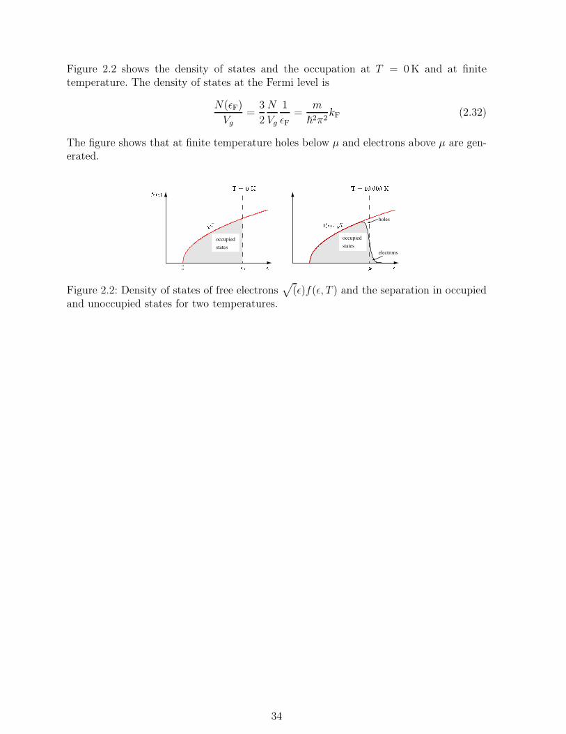
Figure 2.2 shows the density of states and the occupation at T = 0K and at finitetemperature. The density of states at the Fermi level is

N(#F)

Vg=

3

2

N

Vg

1

#F=

m

!2(2kF (2.32)

The figure shows that at finite temperature holes below µ and electrons above µ are gen-erated.

occupiedstates

occupiedstates

electrons

holes

Figure 2.2: Density of states of free electrons'

(#)f(#, T ) and the separation in occupiedand unoccupied states for two temperatures.

34