CS70.

1. Random Variables: Brief Review

2. Joint Distributions.

3. Linearity of Expectation

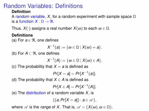
Random Variables: DefinitionsDefinitionA random variable, X , for a random experiment with sample space Ωis a function X : Ω→ℜ.

Thus, X (·) assigns a real number X (ω) to each ω ∈ Ω.

Definitions(a) For a ∈ℜ, one defines

X−1(a) := ω ∈ Ω | X (ω) = a.(b) For A⊂ℜ, one defines

X−1(A) := ω ∈ Ω | X (ω) ∈ A.(c) The probability that X = a is defined as

Pr [X = a] = Pr [X−1(a)].

(d) The probability that X ∈ A is defined as

Pr [X ∈ A] = Pr [X−1(A)].

(e) The distribution of a random variable X , is

(a,Pr [X = a]) : a ∈A ,

where A is the range of X . That is, A = X (ω),ω ∈ Ω.

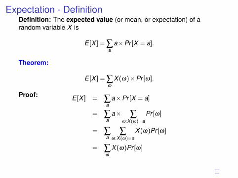
Expectation - DefinitionDefinition: The expected value (or mean, or expectation) of arandom variable X is

E [X ] = ∑a

a×Pr [X = a].

Theorem:

E [X ] = ∑ω

X (ω)×Pr [ω].

Proof: E [X ] = ∑a

a×Pr [X = a]

= ∑a

a× ∑ω:X (ω)=a

Pr [ω]

= ∑a

∑ω:X (ω)=a

X (ω)Pr [ω]

= ∑ω

X (ω)Pr [ω]

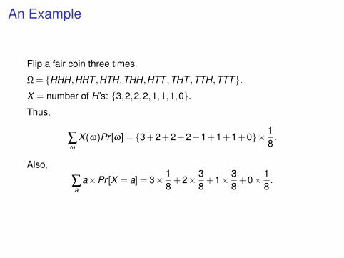
An Example

Flip a fair coin three times.

Ω = HHH,HHT ,HTH,THH,HTT ,THT ,TTH,TTT.X = number of H ’s: 3,2,2,2,1,1,1,0.Thus,

∑ω

X (ω)Pr [ω] = 3 + 2 + 2 + 2 + 1 + 1 + 1 + 0× 18.

Also,

∑a

a×Pr [X = a] = 3× 18

+ 2× 38

+ 1× 38

+ 0× 18.

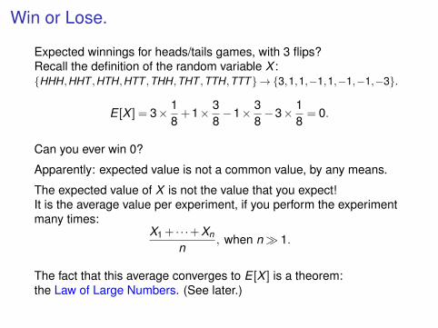
Win or Lose.

Expected winnings for heads/tails games, with 3 flips?Recall the definition of the random variable X :HHH,HHT ,HTH,HTT ,THH,THT ,TTH,TTT→ 3,1,1,−1,1,−1,−1,−3.

E [X ] = 3× 18

+ 1× 38−1× 3

8−3× 1

8= 0.

Can you ever win 0?

Apparently: expected value is not a common value, by any means.

The expected value of X is not the value that you expect!It is the average value per experiment, if you perform the experimentmany times:

X1 + · · ·+ Xn

n, when n 1.

The fact that this average converges to E [X ] is a theorem:the Law of Large Numbers. (See later.)

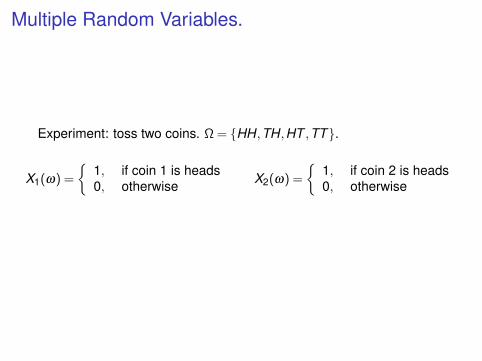
Multiple Random Variables.

Experiment: toss two coins. Ω = HH,TH,HT ,TT.

X1(ω) =

1, if coin 1 is heads0, otherwise X2(ω) =

1, if coin 2 is heads0, otherwise

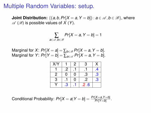
Multiple Random Variables: setup.

Joint Distribution: (a,b,Pr [X = a,Y = b]) : a ∈A ,b ∈B, whereA (B) is possible values of X (Y ).

∑a∈A ,b∈B

Pr [X = a,Y = b] = 1

Marginal for X : Pr [X = a] = ∑b∈B Pr [X = a,Y = b].Marginal for Y : Pr [Y = b] = ∑a∈A Pr [X = a,Y = b].

X/Y 1 2 3 X1 .2 .1 .1 .42 0 0 .3 .33 .1 0 .2 .3Y .3 .1 .2 .6

Conditional Probability: Pr [X = a|Y = b] = Pr [X=a,Y =b]Pr [Y =b] .

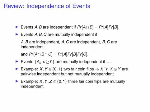
Review: Independence of Events

I Events A,B are independent if Pr [A∩B] = Pr [A]Pr [B].

I Events A,B,C are mutually independent if

A,B are independent, A,C are independent, B,C areindependent

and Pr [A∩B∩C] = Pr [A]Pr [B]Pr [C].

I Events An,n ≥ 0 are mutually independent if . . ..

I Example: X ,Y ∈ 0,1 two fair coin flips⇒ X ,Y ,X ⊕Y arepairwise independent but not mutually independent.

I Example: X ,Y ,Z ∈ 0,1 three fair coin flips are mutuallyindependent.

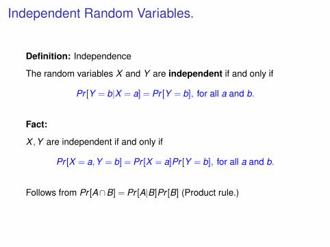
Independent Random Variables.

Definition: Independence

The random variables X and Y are independent if and only if

Pr [Y = b|X = a] = Pr [Y = b], for all a and b.

Fact:

X ,Y are independent if and only if

Pr [X = a,Y = b] = Pr [X = a]Pr [Y = b], for all a and b.

Follows from Pr [A∩B] = Pr [A|B]Pr [B] (Product rule.)

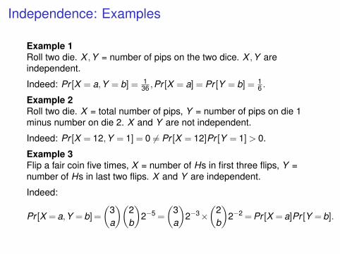
Independence: Examples

Example 1Roll two die. X ,Y = number of pips on the two dice. X ,Y areindependent.

Indeed: Pr [X = a,Y = b] = 136 ,Pr [X = a] = Pr [Y = b] = 1

6 .

Example 2Roll two die. X = total number of pips, Y = number of pips on die 1minus number on die 2. X and Y are not independent.

Indeed: Pr [X = 12,Y = 1] = 0 6= Pr [X = 12]Pr [Y = 1] > 0.

Example 3Flip a fair coin five times, X = number of Hs in first three flips, Y =number of Hs in last two flips. X and Y are independent.

Indeed:

Pr [X = a,Y = b] =

(3a

)(2b

)2−5 =

(3a

)2−3×

(2b

)2−2 = Pr [X = a]Pr [Y = b].

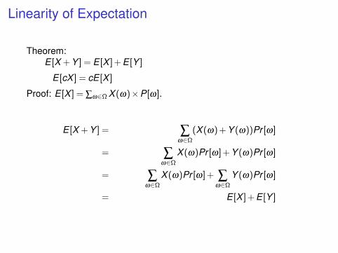
Linearity of Expectation

Theorem:E [X + Y ] = E [X ] + E [Y ]

E [cX ] = cE [X ]

Proof: E [X ] = ∑ω∈Ω X (ω)×P[ω].

E [X + Y ] = ∑ω∈Ω

(X (ω) + Y (ω))Pr [ω]

= ∑ω∈Ω

X (ω)Pr [ω] + Y (ω)Pr [ω]

= ∑ω∈Ω

X (ω)Pr [ω] + ∑ω∈Ω

Y (ω)Pr [ω]

= E [X ] + E [Y ]

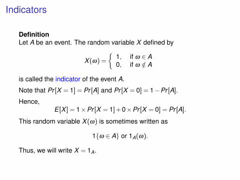
Indicators

DefinitionLet A be an event. The random variable X defined by

X (ω) =

1, if ω ∈ A0, if ω /∈ A

is called the indicator of the event A.

Note that Pr [X = 1] = Pr [A] and Pr [X = 0] = 1−Pr [A].

Hence,E [X ] = 1×Pr [X = 1] + 0×Pr [X = 0] = Pr [A].

This random variable X (ω) is sometimes written as

1ω ∈ A or 1A(ω).

Thus, we will write X = 1A.

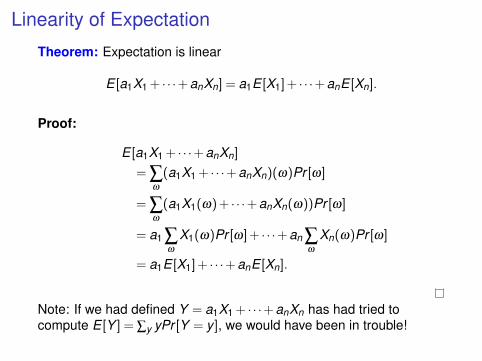
Linearity of Expectation

Theorem: Expectation is linear

E [a1X1 + · · ·+ anXn] = a1E [X1] + · · ·+ anE [Xn].

Proof:

E [a1X1 + · · ·+ anXn]

= ∑ω

(a1X1 + · · ·+ anXn)(ω)Pr [ω]

= ∑ω

(a1X1(ω) + · · ·+ anXn(ω))Pr [ω]

= a1 ∑ω

X1(ω)Pr [ω] + · · ·+ an ∑ω

Xn(ω)Pr [ω]

= a1E [X1] + · · ·+ anE [Xn].

Note: If we had defined Y = a1X1 + · · ·+ anXn has had tried tocompute E [Y ] = ∑y yPr [Y = y ], we would have been in trouble!

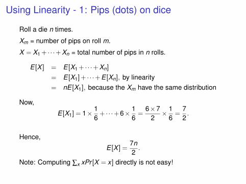
Using Linearity - 1: Pips (dots) on dice

Roll a die n times.

Xm = number of pips on roll m.

X = X1 + · · ·+ Xn = total number of pips in n rolls.

E [X ] = E [X1 + · · ·+ Xn]

= E [X1] + · · ·+ E [Xn], by linearity= nE [X1], because the Xm have the same distribution

Now,

E [X1] = 1× 16

+ · · ·+ 6× 16

=6×7

2× 1

6=

72.

Hence,

E [X ] =7n2.

Note: Computing ∑x xPr [X = x ] directly is not easy!

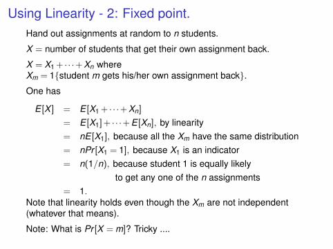
Using Linearity - 2: Fixed point.Hand out assignments at random to n students.

X = number of students that get their own assignment back.

X = X1 + · · ·+ Xn whereXm = 1student m gets his/her own assignment back.One has

E [X ] = E [X1 + · · ·+ Xn]

= E [X1] + · · ·+ E [Xn], by linearity= nE [X1], because all the Xm have the same distribution= nPr [X1 = 1], because X1 is an indicator= n(1/n), because student 1 is equally likely

to get any one of the n assignments= 1.

Note that linearity holds even though the Xm are not independent(whatever that means).

Note: What is Pr [X = m]? Tricky ....

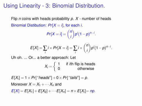
Using Linearity - 3: Binomial Distribution.

Flip n coins with heads probability p. X - number of heads

Binomial Distibution: Pr [X = i], for each i .

Pr [X = i] =

(ni

)pi (1−p)n−i .

E [X ] = ∑i

i×Pr [X = i] = ∑i

i×(

ni

)pi (1−p)n−i .

Uh oh. ... Or... a better approach: Let

Xi =

1 if i th flip is heads0 otherwise

E [Xi ] = 1×Pr [“heads′′] + 0×Pr [“tails′′] = p.

Moreover X = X1 + · · ·Xn and

E [X ] = E [X1] + E [X2] + · · ·E [Xn] = n×E [Xi ]= np.

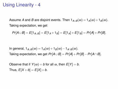
Using Linearity - 4

Assume A and B are disjoint events. Then 1A∪B(ω) = 1A(ω) + 1B(ω).

Taking expectation, we get

Pr [A∪B] = E [1A∪B] = E [1A + 1B] = E [1A] + E [1B] = Pr [A] + Pr [B].

In general, 1A∪B(ω) = 1A(ω) + 1B(ω)−1A∩B(ω).

Taking expectation, we get Pr [A∪B] = Pr [A] + Pr [B]−Pr [A∩B].

Observe that if Y (ω) = b for all ω, then E [Y ] = b.

Thus, E [X + b] = E [X ] + b.

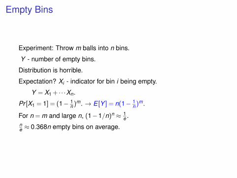
Empty Bins

Experiment: Throw m balls into n bins.

Y - number of empty bins.

Distribution is horrible.

Expectation? Xi - indicator for bin i being empty.

Y = X1 + · · ·Xn.

Pr [X1 = 1] = (1− 1n )m. → E [Y ] = n(1− 1

n )m.

For n = m and large n, (1−1/n)n ≈ 1e .

ne ≈ 0.368n empty bins on average.

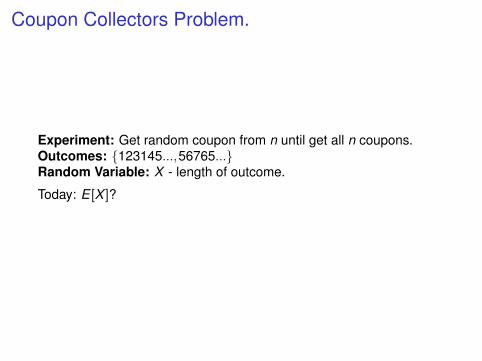
Coupon Collectors Problem.

Experiment: Get random coupon from n until get all n coupons.Outcomes: 123145...,56765...Random Variable: X - length of outcome.

Today: E [X ]?

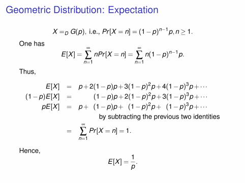
Geometric Distribution: Expectation

X =D G(p), i.e., Pr [X = n] = (1−p)n−1p,n ≥ 1.

One has

E [X ] =∞

∑n=1

nPr [X = n] =∞

∑n=1

n(1−p)n−1p.

Thus,

E [X ] = p + 2(1−p)p + 3(1−p)2p + 4(1−p)3p + · · ·(1−p)E [X ] = (1−p)p + 2(1−p)2p + 3(1−p)3p + · · ·

pE [X ] = p + (1−p)p + (1−p)2p + (1−p)3p + · · ·by subtracting the previous two identities

=∞

∑n=1

Pr [X = n] = 1.

Hence,

E [X ] =1p.

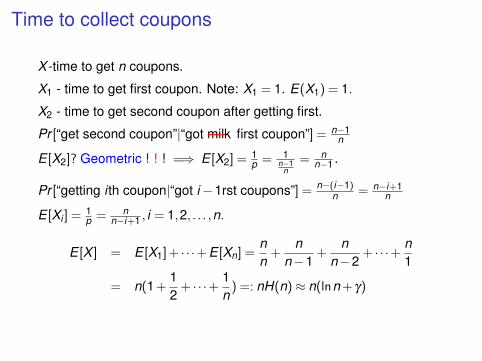
Time to collect coupons

X -time to get n coupons.

X1 - time to get first coupon. Note: X1 = 1. E(X1) = 1.

X2 - time to get second coupon after getting first.

Pr [“get second coupon”|“got milk—- first coupon”] = n−1n

E [X2]? Geometric ! ! ! =⇒ E [X2] = 1p = 1

n−1n

= nn−1 .

Pr [“getting i th coupon|“got i−1rst coupons”] = n−(i−1)n = n−i+1

n

E [Xi ] = 1p = n

n−i+1 , i = 1,2, . . . ,n.

E [X ] = E [X1] + · · ·+ E [Xn] =nn

+n

n−1+

nn−2

+ · · ·+ n1

= n(1 +12

+ · · ·+ 1n

) =: nH(n)≈ n(lnn + γ)

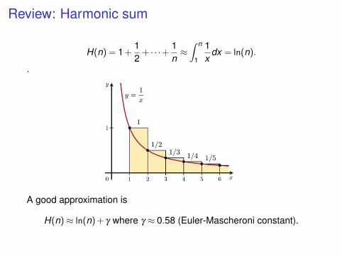
Review: Harmonic sum

H(n) = 1 +12

+ · · ·+ 1n≈∫ n

1

1x

dx = ln(n).

.

A good approximation is

H(n)≈ ln(n) + γ where γ ≈ 0.58 (Euler-Mascheroni constant).

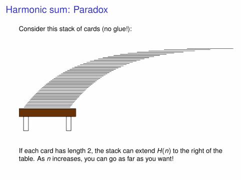
Harmonic sum: Paradox

Consider this stack of cards (no glue!):

If each card has length 2, the stack can extend H(n) to the right of thetable. As n increases, you can go as far as you want!

Paradox

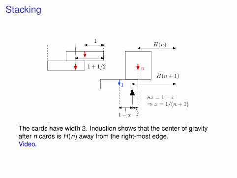
Stacking

The cards have width 2. Induction shows that the center of gravityafter n cards is H(n) away from the right-most edge.Video.

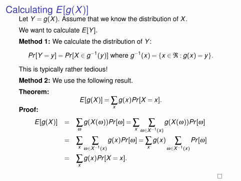
Calculating E [g(X )]Let Y = g(X ). Assume that we know the distribution of X .

We want to calculate E [Y ].

Method 1: We calculate the distribution of Y :

Pr [Y = y ] = Pr [X ∈ g−1(y)] where g−1(x) = x ∈ℜ : g(x) = y.

This is typically rather tedious!

Method 2: We use the following result.

Theorem:E [g(X )] = ∑

xg(x)Pr [X = x ].

Proof:

E [g(X )] = ∑ω

g(X (ω))Pr [ω] = ∑x

∑ω∈X−1(x)

g(X (ω))Pr [ω]

= ∑x

∑ω∈X−1(x)

g(x)Pr [ω] = ∑x

g(x) ∑ω∈X−1(x)

Pr [ω]

= ∑x

g(x)Pr [X = x ].

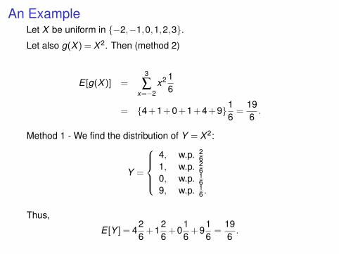
An ExampleLet X be uniform in −2,−1,0,1,2,3.Let also g(X ) = X 2. Then (method 2)

E [g(X )] =3

∑x=−2

x2 16

= 4 + 1 + 0 + 1 + 4 + 916

=196.

Method 1 - We find the distribution of Y = X 2:

Y =

4, w.p. 2

61, w.p. 2

60, w.p. 1

69, w.p. 1

6 .

Thus,

E [Y ] = 426

+ 126

+ 016

+ 916

=196.

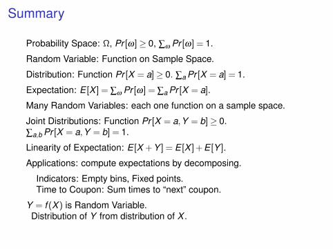
Summary

Probability Space: Ω, Pr [ω]≥ 0, ∑ω Pr [ω] = 1.

Random Variable: Function on Sample Space.

Distribution: Function Pr [X = a]≥ 0. ∑a Pr [X = a] = 1.

Expectation: E [X ] = ∑ω Pr [ω] = ∑a Pr [X = a].

Many Random Variables: each one function on a sample space.

Joint Distributions: Function Pr [X = a,Y = b]≥ 0.∑a,b Pr [X = a,Y = b] = 1.

Linearity of Expectation: E [X + Y ] = E [X ] + E [Y ].

Applications: compute expectations by decomposing.

Indicators: Empty bins, Fixed points.Time to Coupon: Sum times to “next” coupon.

Y = f (X ) is Random Variable.Distribution of Y from distribution of X .