Numerical Evaluation of Standard Distributions in Random ...
48
Numerical Evaluation of Standard Distributions in Random Matrix Theory A Review of Folkmar Bornemann’s MATLAB Package and Paper Matt Redmond Department of Mathematics Massachusetts Institute of Technology Cambridge, MA 02139, USA May 15, 2013 M. Redmond MIT Numerical Evaluation of Standard Distributions in Random Matrix Theory
Transcript of Numerical Evaluation of Standard Distributions in Random ...

Numerical Evaluation of Standard Distributionsin Random Matrix Theory
A Review of Folkmar Bornemann’s MATLAB Package and Paper
Matt Redmond
Department of MathematicsMassachusetts Institute of Technology
Cambridge, MA 02139, USA
May 15, 2013
M. Redmond MIT
Numerical Evaluation of Standard Distributions in Random Matrix Theory
Level Spacing Function
Definition (Gaussian Ensemble Spacing Function)Let J ⊂ R be an open interval.
E(n)β (k; J) ≡ P(k eigenvalues of the n × n Gaussian β-ensemble lie in J)
Let J = (0, s). Then E2(0; J) = probability no eigenvalues lie in (0, s).
M. Redmond MIT
Numerical Evaluation of Standard Distributions in Random Matrix Theory
Fredholm Determinant
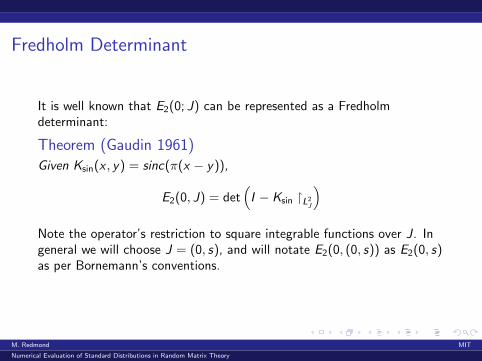
It is well known that E2(0; J) can be represented as a Fredholmdeterminant:
Theorem (Gaudin 1961)Given Ksin(x , y) = sinc(π(x − y)),
E2(0, J) = det(I − Ksin �L2
J
)Note the operator’s restriction to square integrable functions over J. Ingeneral we will choose J = (0, s), and will notate E2(0, (0, s)) as E2(0, s)as per Bornemann’s conventions.
M. Redmond MIT
Numerical Evaluation of Standard Distributions in Random Matrix Theory
Fredholm Determinant
It is well known that E2(0; J) can be represented as a Fredholmdeterminant:
Theorem (Gaudin 1961)Given Ksin(x , y) = sinc(π(x − y)),
E2(0, J) = det(I − Ksin �L2
J
)Note the operator’s restriction to square integrable functions over J. Ingeneral we will choose J = (0, s), and will notate E2(0, (0, s)) as E2(0, s)as per Bornemann’s conventions.
M. Redmond MIT
Numerical Evaluation of Standard Distributions in Random Matrix Theory
Integral Formulation
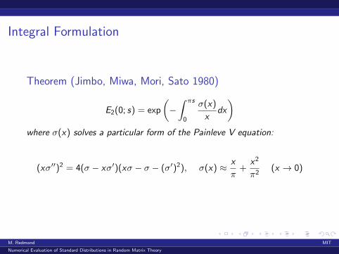
Theorem (Jimbo, Miwa, Mori, Sato 1980)
E2(0; s) = exp
(−∫ πs
0
σ(x)
xdx
)where σ(x) solves a particular form of the Painleve V equation:
(xσ′′)2 = 4(σ − xσ′)(xσ − σ − (σ′)2), σ(x) ≈ x
π+
x2
π2(x → 0)
M. Redmond MIT
Numerical Evaluation of Standard Distributions in Random Matrix Theory
Tracy-Widom Distribution
Definition (Tracy-Widom Distribution)Let F2(s) ≡ P( no eigenvalues of large-matrix limit GUE lie in (s,∞))
M. Redmond MIT
Numerical Evaluation of Standard Distributions in Random Matrix Theory
Tracy-Widom Distribution
Definition (Tracy-Widom Distribution)Let F2(s) ≡ P( no eigenvalues of large-matrix limit GUE lie in (s,∞))
M. Redmond MIT
Numerical Evaluation of Standard Distributions in Random Matrix Theory
Determinantal Representation
Theorem (Bronk 1964)Given
KAi(x , y) =Ai(x)Ai’(y)− Ai’(x)Ai(y)
x − y
we haveF2(s) = det
(I − KAi �L2
(s,∞)
)
M. Redmond MIT
Numerical Evaluation of Standard Distributions in Random Matrix Theory
Determinantal Representation
Theorem (Bronk 1964)Given
KAi(x , y) =Ai(x)Ai’(y)− Ai’(x)Ai(y)
x − y
we haveF2(s) = det
(I − KAi �L2
(s,∞)
)
M. Redmond MIT
Numerical Evaluation of Standard Distributions in Random Matrix Theory
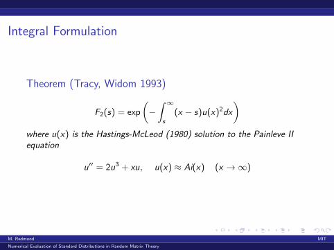
Integral Formulation
Theorem (Tracy, Widom 1993)
F2(s) = exp
(−∫ ∞s
(x − s)u(x)2dx
)where u(x) is the Hastings-McLeod (1980) solution to the Painleve IIequation
u′′ = 2u3 + xu, u(x) ≈ Ai(x) (x →∞)
M. Redmond MIT
Numerical Evaluation of Standard Distributions in Random Matrix Theory
Integral Formulation
Theorem (Tracy, Widom 1993)
F2(s) = exp
(−∫ ∞s
(x − s)u(x)2dx
)where u(x) is the Hastings-McLeod (1980) solution to the Painleve IIequation
u′′ = 2u3 + xu, u(x) ≈ Ai(x) (x →∞)
M. Redmond MIT
Numerical Evaluation of Standard Distributions in Random Matrix Theory
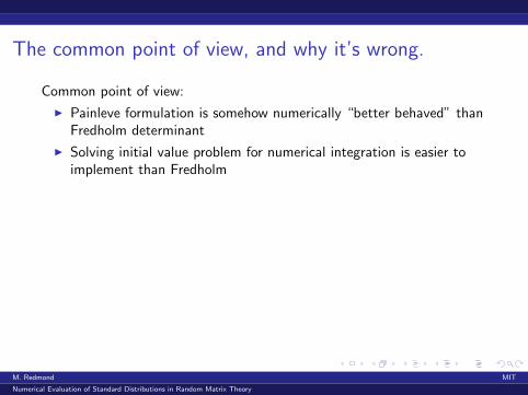
The common point of view, and why it’s wrong.
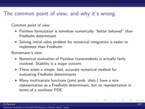
Common point of view:
I Painleve formulation is somehow numerically “better behaved” thanFredholm determinant
I Solving initial value problem for numerical integration is easier toimplement than Fredholm
Bornemann’s view:
I Numerical evaluation of Painleve transcendents is actually fairlyinvolved. Stability is a major concern.
I There exists a simple, fast, accurate numerical method forevaluating Fredholm determinants
I Many multivariate functions (joint prob. dists.) have a nicerepresentation as a Fredholm determinant, but no representation interms of a nonlinear PDE.
M. Redmond MIT
Numerical Evaluation of Standard Distributions in Random Matrix Theory
The common point of view, and why it’s wrong.
Common point of view:
I Painleve formulation is somehow numerically “better behaved” thanFredholm determinant
I Solving initial value problem for numerical integration is easier toimplement than Fredholm
Bornemann’s view:
I Numerical evaluation of Painleve transcendents is actually fairlyinvolved. Stability is a major concern.
I There exists a simple, fast, accurate numerical method forevaluating Fredholm determinants
I Many multivariate functions (joint prob. dists.) have a nicerepresentation as a Fredholm determinant, but no representation interms of a nonlinear PDE.
M. Redmond MIT
Numerical Evaluation of Standard Distributions in Random Matrix Theory
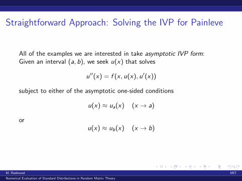
Straightforward Approach: Solving the IVP for Painleve
All of the examples we are interested in take asymptotic IVP form:Given an interval (a, b), we seek u(x) that solves
u′′(x) = f (x , u(x), u′(x))
subject to either of the asymptotic one-sided conditions
u(x) ≈ ua(x) (x → a)
oru(x) ≈ ub(x) (x → b)
M. Redmond MIT
Numerical Evaluation of Standard Distributions in Random Matrix Theory
Straightforward Approach: Solving the IVP for Painleve
All of the examples we are interested in take asymptotic IVP form:
Given an interval (a, b), we seek u(x) that solves
u′′(x) = f (x , u(x), u′(x))
subject to either of the asymptotic one-sided conditions
u(x) ≈ ua(x) (x → a)
oru(x) ≈ ub(x) (x → b)
M. Redmond MIT
Numerical Evaluation of Standard Distributions in Random Matrix Theory
Straightforward Approach: Solving the IVP for Painleve
All of the examples we are interested in take asymptotic IVP form:Given an interval (a, b), we seek u(x) that solves
u′′(x) = f (x , u(x), u′(x))
subject to either of the asymptotic one-sided conditions
u(x) ≈ ua(x) (x → a)
oru(x) ≈ ub(x) (x → b)
M. Redmond MIT
Numerical Evaluation of Standard Distributions in Random Matrix Theory
Straightforward Approach (cont.)
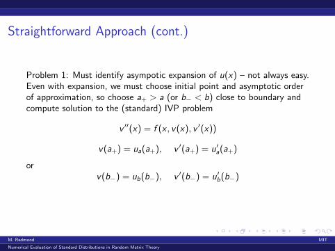
Problem 1: Must identify asympotic expansion of u(x) – not always easy.Even with expansion, we must choose initial point and asymptotic orderof approximation, so choose a+ > a (or b− < b) close to boundary andcompute solution to the (standard) IVP problem
v ′′(x) = f (x , v(x), v ′(x))
v(a+) = ua(a+), v ′(a+) = u′a(a+)
orv(b−) = ub(b−), v ′(b−) = u′b(b−)
M. Redmond MIT
Numerical Evaluation of Standard Distributions in Random Matrix Theory
Straightforward Approach (cont.)
Problem 1: Must identify asympotic expansion of u(x) – not always easy.
Even with expansion, we must choose initial point and asymptotic orderof approximation, so choose a+ > a (or b− < b) close to boundary andcompute solution to the (standard) IVP problem
v ′′(x) = f (x , v(x), v ′(x))
v(a+) = ua(a+), v ′(a+) = u′a(a+)
orv(b−) = ub(b−), v ′(b−) = u′b(b−)
M. Redmond MIT
Numerical Evaluation of Standard Distributions in Random Matrix Theory
Straightforward Approach (cont.)
Problem 1: Must identify asympotic expansion of u(x) – not always easy.Even with expansion, we must choose initial point and asymptotic orderof approximation, so choose a+ > a (or b− < b) close to boundary andcompute solution to the (standard) IVP problem
v ′′(x) = f (x , v(x), v ′(x))
v(a+) = ua(a+), v ′(a+) = u′a(a+)
orv(b−) = ub(b−), v ′(b−) = u′b(b−)
M. Redmond MIT
Numerical Evaluation of Standard Distributions in Random Matrix Theory

Straightforward Approach (cont.)
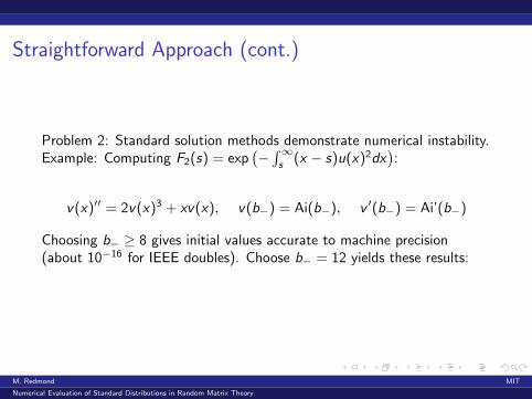
Problem 2: Standard solution methods demonstrate numerical instability.Example: Computing F2(s) = exp
(−∫∞s
(x − s)u(x)2dx):
v(x)′′ = 2v(x)3 + xv(x), v(b−) = Ai(b−), v ′(b−) = Ai’(b−)
Choosing b− ≥ 8 gives initial values accurate to machine precision(about 10−16 for IEEE doubles). Choose b− = 12 yields these results:
M. Redmond MIT
Numerical Evaluation of Standard Distributions in Random Matrix Theory
Straightforward Approach (cont.)
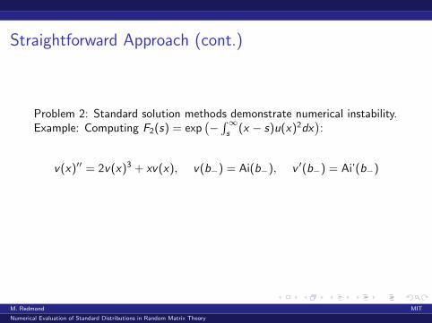
Problem 2: Standard solution methods demonstrate numerical instability.
Example: Computing F2(s) = exp(−∫∞s
(x − s)u(x)2dx):
v(x)′′ = 2v(x)3 + xv(x), v(b−) = Ai(b−), v ′(b−) = Ai’(b−)
Choosing b− ≥ 8 gives initial values accurate to machine precision(about 10−16 for IEEE doubles). Choose b− = 12 yields these results:
M. Redmond MIT
Numerical Evaluation of Standard Distributions in Random Matrix Theory
Straightforward Approach (cont.)
Problem 2: Standard solution methods demonstrate numerical instability.Example: Computing F2(s) = exp
(−∫∞s
(x − s)u(x)2dx):
v(x)′′ = 2v(x)3 + xv(x), v(b−) = Ai(b−), v ′(b−) = Ai’(b−)
Choosing b− ≥ 8 gives initial values accurate to machine precision(about 10−16 for IEEE doubles). Choose b− = 12 yields these results:
M. Redmond MIT
Numerical Evaluation of Standard Distributions in Random Matrix Theory
Straightforward Approach (cont.)
Problem 2: Standard solution methods demonstrate numerical instability.Example: Computing F2(s) = exp
(−∫∞s
(x − s)u(x)2dx):
v(x)′′ = 2v(x)3 + xv(x), v(b−) = Ai(b−), v ′(b−) = Ai’(b−)
Choosing b− ≥ 8 gives initial values accurate to machine precision(about 10−16 for IEEE doubles). Choose b− = 12 yields these results:
M. Redmond MIT
Numerical Evaluation of Standard Distributions in Random Matrix Theory
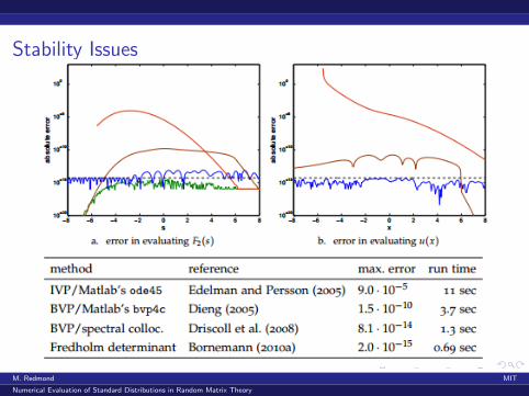
Stability Issues
M. Redmond MIT
Numerical Evaluation of Standard Distributions in Random Matrix Theory
Less Straightforward Approach: Solving the BVP forPainleve
Stability issues described in depth in Bornemann’s paper lead to a BVPapproach.We use asymptotic expression ua(x) at (x → a) to infer asymptoticexpression ub(x) at (x → b), or vice versa.Approximate u(x) by solving BVP:
v ′′(x) = f (x , v(x), v ′(x)), v(a+) = ua(a+), v(b−) = ub(b−)
Requires four choices: values of a+, b−, and order of asymptoticaccuracy for ua(x) and ub(x)
M. Redmond MIT
Numerical Evaluation of Standard Distributions in Random Matrix Theory
Less Straightforward Approach: An Example
Computing F2(s) via computation of u(x) via BVP methods:By definition, u(x) ≈ Ai(x) (x →∞) so we take ub(x) = Ai(x).Choose a+ = −10, b− = 6 (Dieng, 2005).We need to choose a sufficiently accurate asymptotic expansion forua(x). Tracy and Widom show
u(x) =
√−x
2
(1 +
1
8x−3 − 73
128x−6 +
10657
1024x−9 + O(x−12)
), (x → −∞)
so we’ll use that for ua(x).
M. Redmond MIT
Numerical Evaluation of Standard Distributions in Random Matrix Theory
Less Straightforward Approach: An Example
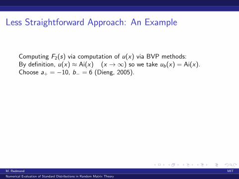
Computing F2(s) via computation of u(x) via BVP methods:
By definition, u(x) ≈ Ai(x) (x →∞) so we take ub(x) = Ai(x).Choose a+ = −10, b− = 6 (Dieng, 2005).We need to choose a sufficiently accurate asymptotic expansion forua(x). Tracy and Widom show
u(x) =
√−x
2
(1 +
1
8x−3 − 73
128x−6 +
10657
1024x−9 + O(x−12)
), (x → −∞)
so we’ll use that for ua(x).
M. Redmond MIT
Numerical Evaluation of Standard Distributions in Random Matrix Theory
Less Straightforward Approach: An Example
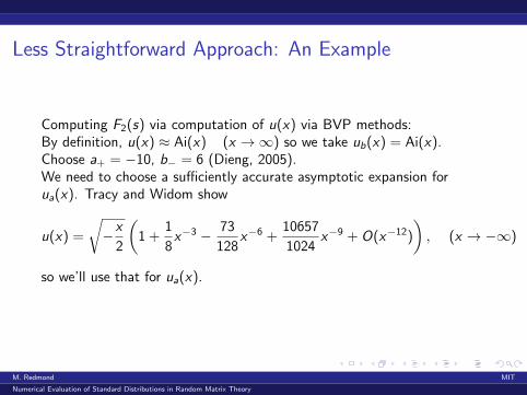
Computing F2(s) via computation of u(x) via BVP methods:By definition, u(x) ≈ Ai(x) (x →∞) so we take ub(x) = Ai(x).Choose a+ = −10, b− = 6 (Dieng, 2005).
We need to choose a sufficiently accurate asymptotic expansion forua(x). Tracy and Widom show
u(x) =
√−x
2
(1 +
1
8x−3 − 73
128x−6 +
10657
1024x−9 + O(x−12)
), (x → −∞)
so we’ll use that for ua(x).
M. Redmond MIT
Numerical Evaluation of Standard Distributions in Random Matrix Theory
Less Straightforward Approach: An Example
Computing F2(s) via computation of u(x) via BVP methods:By definition, u(x) ≈ Ai(x) (x →∞) so we take ub(x) = Ai(x).Choose a+ = −10, b− = 6 (Dieng, 2005).We need to choose a sufficiently accurate asymptotic expansion forua(x). Tracy and Widom show
u(x) =
√−x
2
(1 +
1
8x−3 − 73
128x−6 +
10657
1024x−9 + O(x−12)
), (x → −∞)
so we’ll use that for ua(x).
M. Redmond MIT
Numerical Evaluation of Standard Distributions in Random Matrix Theory

Stability Issues
M. Redmond MIT
Numerical Evaluation of Standard Distributions in Random Matrix Theory
Pitfalls of BVP approach
I Require turning asymptotic expansion at one endpoint intoasymptotic endpoint at other point. Not easy!
I Selecting appropriate a+ and b− along with indices of truncation is abit of a black art.
I Actually solving BVP requires choosing starting values for Newtoniteration, discretizing the DE, choosing a good step size, etc.
Punchline: BVP approach is insufficiently ”black-box” for us.
M. Redmond MIT
Numerical Evaluation of Standard Distributions in Random Matrix Theory
Better Approach: Numerical Evaluation of FredholmDeterminants
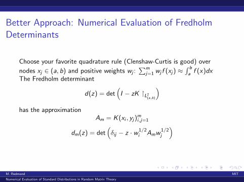
Choose your favorite quadrature rule (Clenshaw-Curtis is good) over
nodes xj ∈ (a, b) and positive weights wj :∑m
j=1 wj f (xj) ≈∫ b
af (x)dx
The Fredholm determinant
d(z) = det(I − zK �L2
(a,b)
)has the approximation
Am = K (xi , yj)mi,j=1
dm(z) = det(δij − z · w1/2
i Amw1/2j
)
M. Redmond MIT
Numerical Evaluation of Standard Distributions in Random Matrix Theory
Better Approach: Numerical Evaluation of FredholmDeterminants
Choose your favorite quadrature rule (Clenshaw-Curtis is good) over
nodes xj ∈ (a, b) and positive weights wj :∑m
j=1 wj f (xj) ≈∫ b
af (x)dx
The Fredholm determinant
d(z) = det(I − zK �L2
(a,b)
)has the approximation
Am = K (xi , yj)mi,j=1
dm(z) = det(δij − z · w1/2
i Amw1/2j
)
M. Redmond MIT
Numerical Evaluation of Standard Distributions in Random Matrix Theory
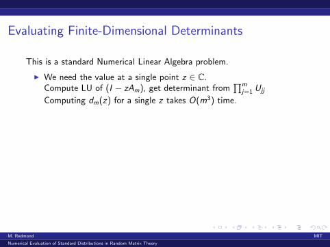
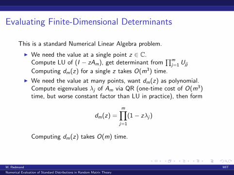
Evaluating Finite-Dimensional Determinants
This is a standard Numerical Linear Algebra problem.
I We need the value at a single point z ∈ C.Compute LU of (I − zAm), get determinant from
∏mj=1 Ujj
Computing dm(z) for a single z takes O(m3) time.
I We need the value at many points, want dm(z) as polynomial.Compute eigenvalues λj of Am via QR (one-time cost of O(m3)time, but worse constant factor than LU in practice), then form
dm(z) =m∏j=1
(1− zλj)
Computing dm(z) takes O(m) time.
M. Redmond MIT
Numerical Evaluation of Standard Distributions in Random Matrix Theory
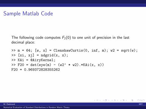
Sample Matlab Code
The following code computes F2(0) to one unit of precision in the lastdecimal place:
>> m = 64; [w, x] = ClenshawCurtis(0, inf, m); w2 = sqrt(w);
>> [xi, xj] = ndgrid(x, x);
>> KAi = @AiryKernel;
>> F20 = det(eye(m) - (w2’ * w2).*KAi(x, x))
F20 = 0.969372828355262
M. Redmond MIT
Numerical Evaluation of Standard Distributions in Random Matrix Theory
Wrapup
I Computing Fredholm Determinants is faster, easier, and more stablethan integrating Painleve IVP or BVP.
I Being able to handle things that are expressed in non-PDE form isuseful.
I Bornemann uses the toolset to identify (and subsequently prove)several new results (omitted here for brevity) about distributions ofthe k-th largest eigenvalue in the soft-edge scaling limit of the GOEand GSE – the numerical code generates immediate insights!
M. Redmond MIT
Numerical Evaluation of Standard Distributions in Random Matrix Theory