Today

1. Probability

2. Random variables

CS 8803-MDM Lecture 2 – p. 3/20

Probability

We won’t spend that much time on it, but we need to starthere.

CS 8803-MDM Lecture 2 – p. 4/20

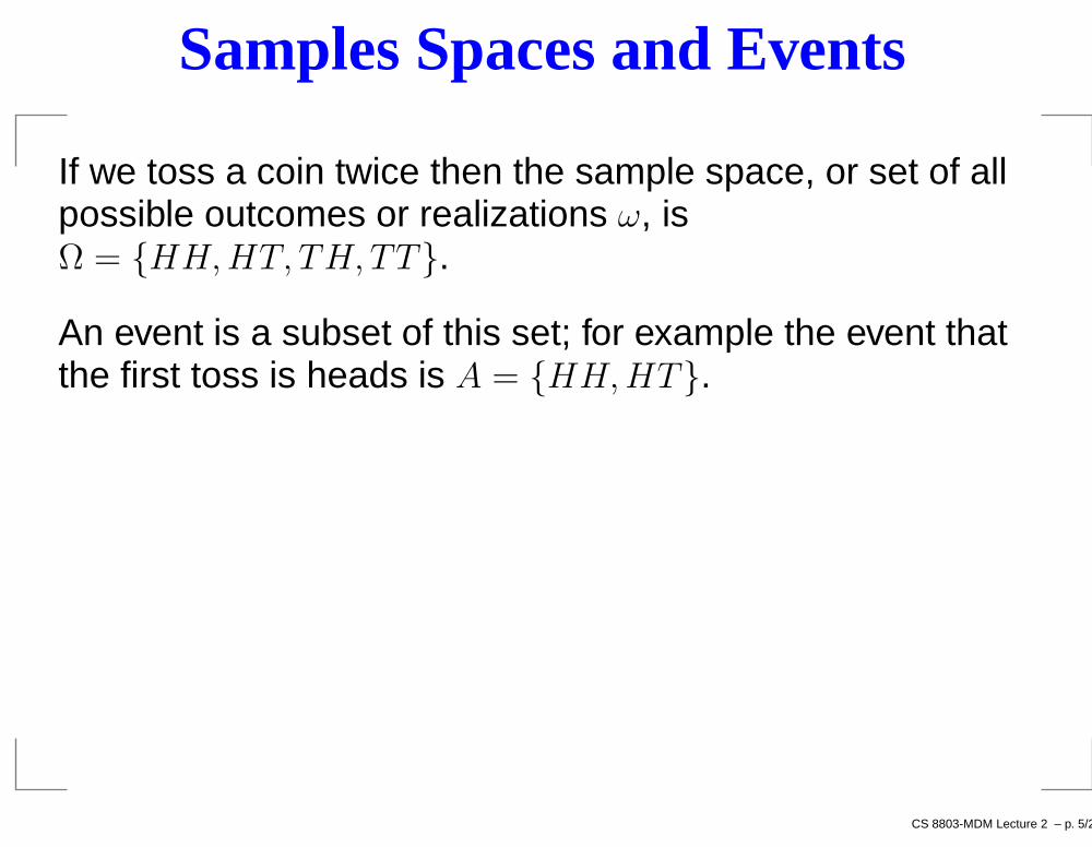
Samples Spaces and Events

If we toss a coin twice then the sample space, or set of allpossible outcomes or realizations ω, isΩ = {HH,HT, TH, TT}.

An event is a subset of this set; for example the event thatthe first toss is heads is A = {HH,HT}.

CS 8803-MDM Lecture 2 – p. 5/20

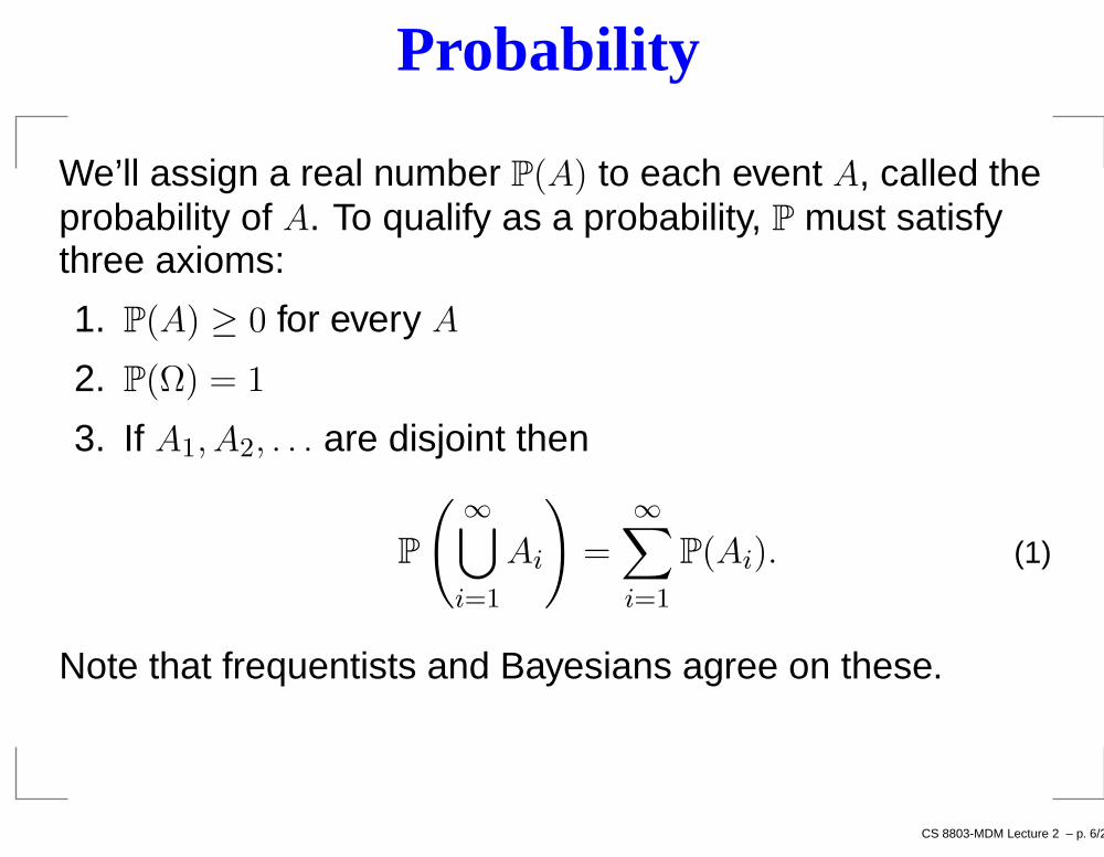
Probability

We’ll assign a real number P(A) to each event A, called theprobability of A. To qualify as a probability, P must satisfythree axioms:

1. P(A) ≥ 0 for every A2. P(Ω) = 1

3. If A1, A2, . . . are disjoint then

P

(∞⋃

i=1

Ai

)

=

∞∑

i=1

P(Ai). (1)

Note that frequentists and Bayesians agree on these.

CS 8803-MDM Lecture 2 – p. 6/20

Random VariablesThis is where we start talking about data.

CS 8803-MDM Lecture 2 – p. 7/20

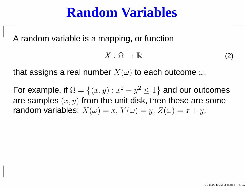
Random Variables

A random variable is a mapping, or function

X : Ω → R (2)

that assigns a real number X(ω) to each outcome ω.

For example, if Ω ={(x, y) : x2 + y2 ≤ 1

}and our outcomes

are samples (x, y) from the unit disk, then these are somerandom variables: X(ω) = x, Y (ω) = y, Z(ω) = x + y.

CS 8803-MDM Lecture 2 – p. 8/20

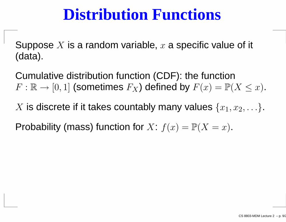
Distribution Functions

Suppose X is a random variable, x a specific value of it(data).

Cumulative distribution function (CDF): the functionF : R → [0, 1] (sometimes FX) defined by F (x) = P(X ≤ x).

X is discrete if it takes countably many values {x1, x2, . . .}.

Probability (mass) function for X: f(x) = P(X = x).

CS 8803-MDM Lecture 2 – p. 9/20

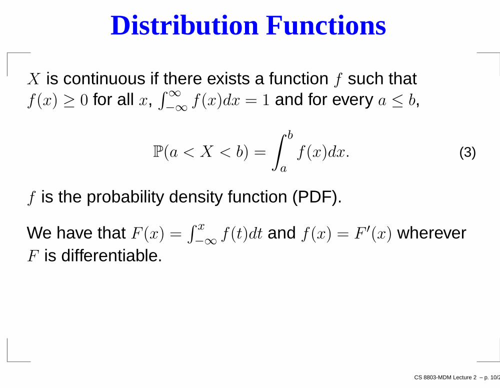
Distribution Functions

X is continuous if there exists a function f such thatf(x) ≥ 0 for all x,

∫∞

−∞f(x)dx = 1 and for every a ≤ b,

P(a < X < b) =

∫ b

a

f(x)dx. (3)

f is the probability density function (PDF).

We have that F (x) =∫ x−∞

f(t)dt and f(x) = F ′(x) whereverF is differentiable.

CS 8803-MDM Lecture 2 – p. 10/20

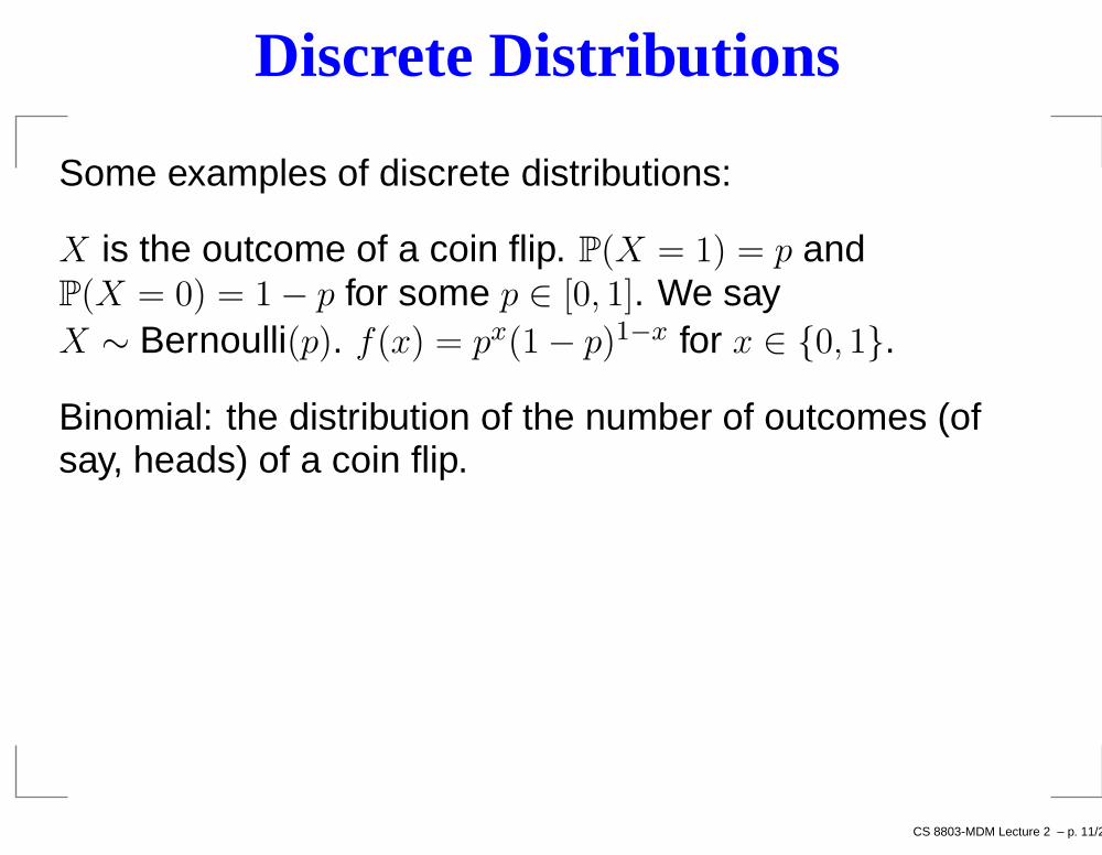
Discrete Distributions

Some examples of discrete distributions:

X is the outcome of a coin flip. P(X = 1) = p andP(X = 0) = 1 − p for some p ∈ [0, 1]. We sayX ∼ Bernoulli(p). f(x) = px(1 − p)1−x for x ∈ {0, 1}.

Binomial: the distribution of the number of outcomes (ofsay, heads) of a coin flip.

CS 8803-MDM Lecture 2 – p. 11/20

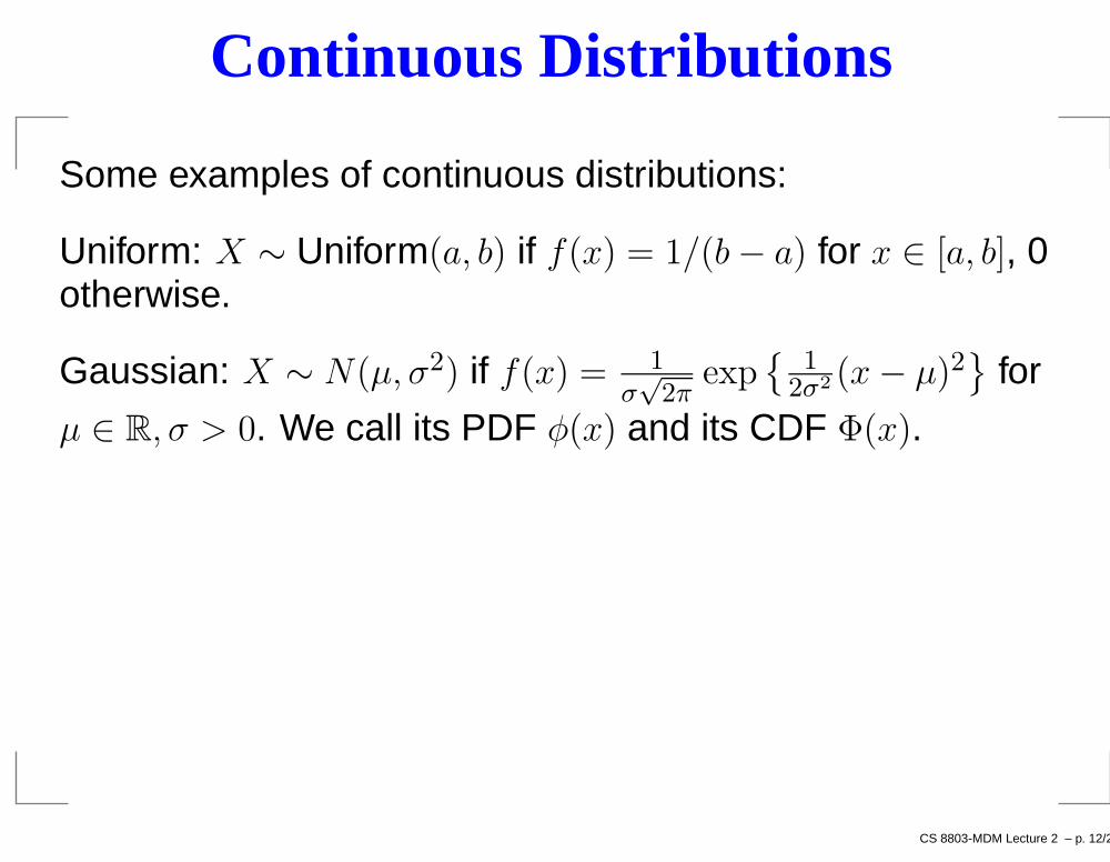
Continuous Distributions

Some examples of continuous distributions:

Uniform: X ∼ Uniform(a, b) if f(x) = 1/(b − a) for x ∈ [a, b], 0otherwise.

Gaussian: X ∼ N(µ, σ2) if f(x) = 1σ√

2πexp

{1

2σ2 (x − µ)2}

for

µ ∈ R, σ > 0. We call its PDF φ(x) and its CDF Φ(x).

CS 8803-MDM Lecture 2 – p. 12/20

Multivariate Distributions

Can define a distribution over a vector of random variables.We say this is a multivariate distribution.

Our dataset generally consists of samples from amultivariate distribution. Each of the columns is a randomvariable. We can also consider the whole vector of randomvariables as a random variable.

CS 8803-MDM Lecture 2 – p. 13/20

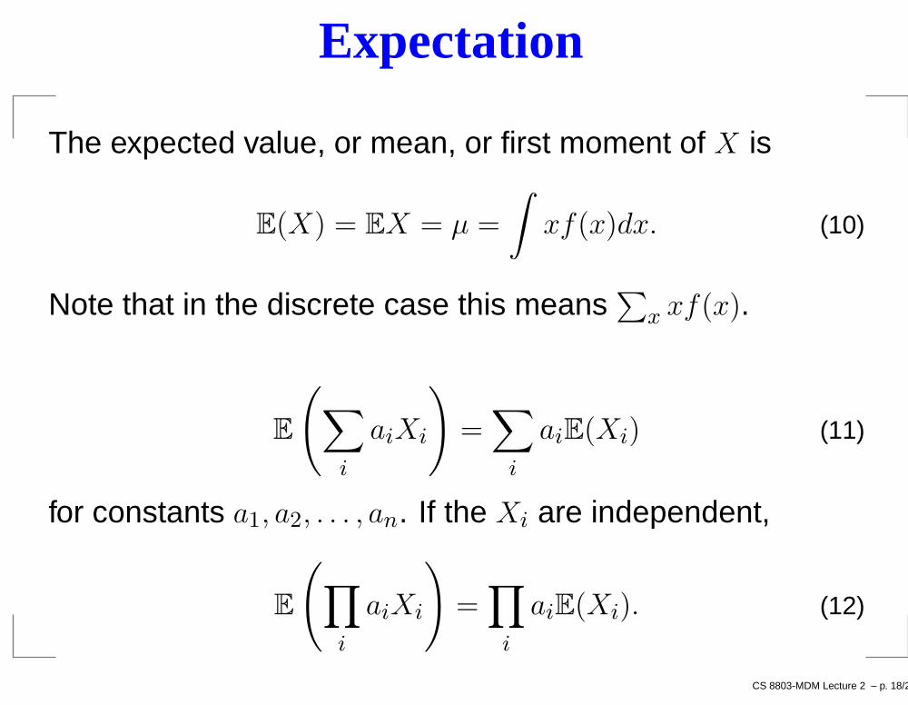
Expectation

The expected value, or mean, or first moment of X is

E(X) = EX = µ =

∫xf(x)dx. (10)

Note that in the discrete case this means∑

x xf(x).

E

(∑

i

aiXi

)=∑

i

aiE(Xi) (11)

for constants a1, a2, . . . , an. If the Xi are independent,

E

(∏

i

aiXi

)=∏

i

aiE(Xi). (12)

CS 8803-MDM Lecture 2 – p. 18/20

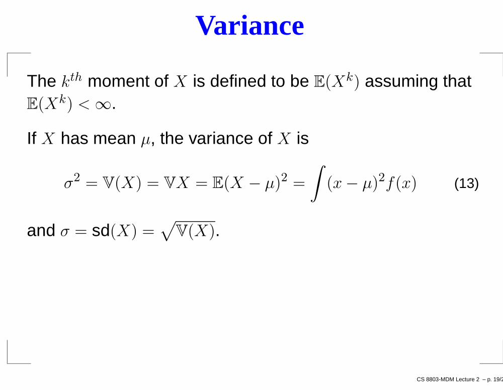
Variance

The kth moment of X is defined to be E(Xk) assuming thatE(Xk) < ∞.

If X has mean µ, the variance of X is

σ2 = V(X) = VX = E(X − µ)2 =∫

(x − µ)2f(x) (13)

and σ = sd(X) =√

V(X).

CS 8803-MDM Lecture 2 – p. 19/20

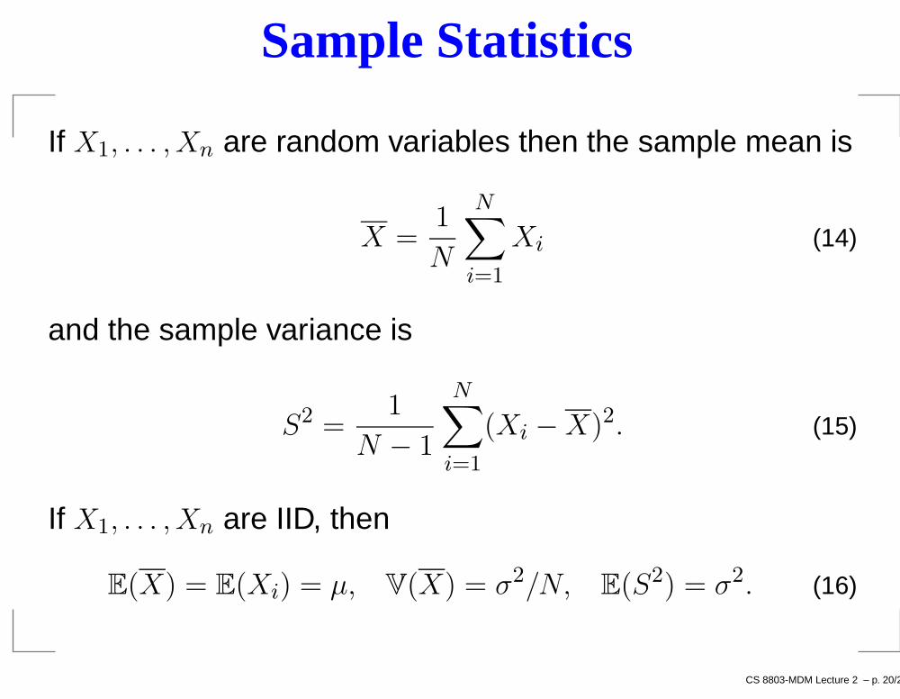
Sample Statistics

If X1, . . . , Xn are random variables then the sample mean is

X =1

N

N∑

i=1

Xi (14)

and the sample variance is

S2 =1

N − 1

N∑

i=1

(Xi − X)2. (15)

If X1, . . . , Xn are IID, then

E(X) = E(Xi) = µ, V(X) = σ2/N, E(S2) = σ2. (16)

CS 8803-MDM Lecture 2 – p. 20/20

Today

1. Some inequalities

2. Asymptotic theory

3. Point estimation

CS 8803-MDM Lecture 3 – p. 2/32

Some inequalities

A few very useful inequalities that will come up in manycontexts – in particular, they lie at the heart of learningtheory.

CS 8803-MDM Lecture 3 – p. 3/32

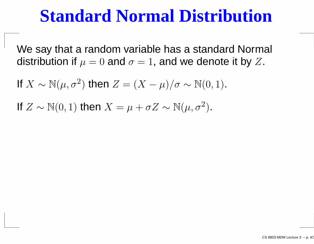
Standard Normal Distribution

We say that a random variable has a standard Normaldistribution if µ = 0 and σ = 1, and we denote it by Z.

If X ∼ N(µ, σ2) then Z = (X − µ)/σ ∼ N(0, 1).

If Z ∼ N(0, 1) then X = µ + σZ ∼ N(µ, σ2).

CS 8803-MDM Lecture 3 – p. 4/32

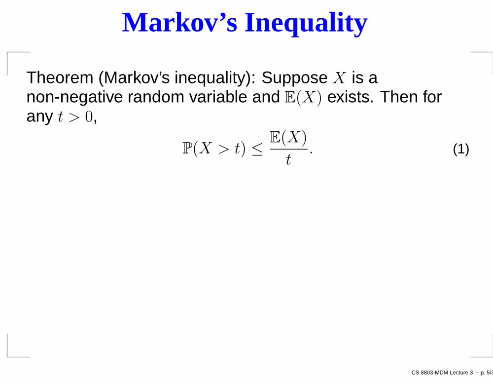
Markov’s Inequality

Theorem (Markov’s inequality): Suppose X is anon-negative random variable and E(X) exists. Then forany t > 0,

P(X > t) ≤ E(X)t

. (1)

CS 8803-MDM Lecture 3 – p. 5/32

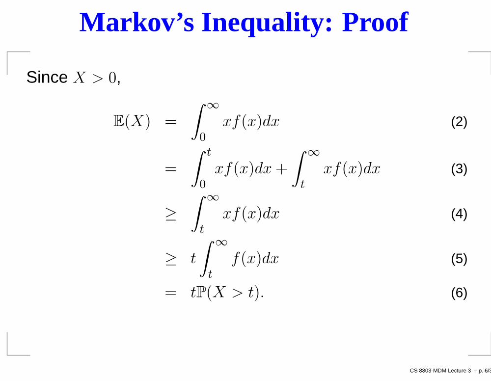
Markov’s Inequality: Proof

Since X > 0,

E(X) =

∫∞

0xf(x)dx (2)

=

∫ t

0xf(x)dx +

∫∞

t

xf(x)dx (3)

≥∫

∞

t

xf(x)dx (4)

≥ t∫

∞

t

f(x)dx (5)

= tP(X > t). (6)

CS 8803-MDM Lecture 3 – p. 6/32

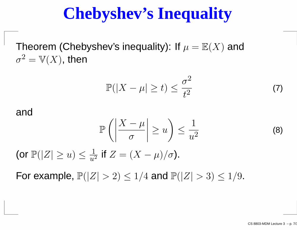
Chebyshev’s Inequality

Theorem (Chebyshev’s inequality): If µ = E(X) andσ2 = V(X), then

P(|X − µ| ≥ t) ≤ σ2

t2(7)

and

P

(∣∣∣∣X − µ

σ

∣∣∣∣ ≥ u)

≤ 1u2

(8)

(or P(|Z| ≥ u) ≤ 1u2

if Z = (X − µ)/σ).

For example, P(|Z| > 2) ≤ 1/4 and P(|Z| > 3) ≤ 1/9.

CS 8803-MDM Lecture 3 – p. 7/32

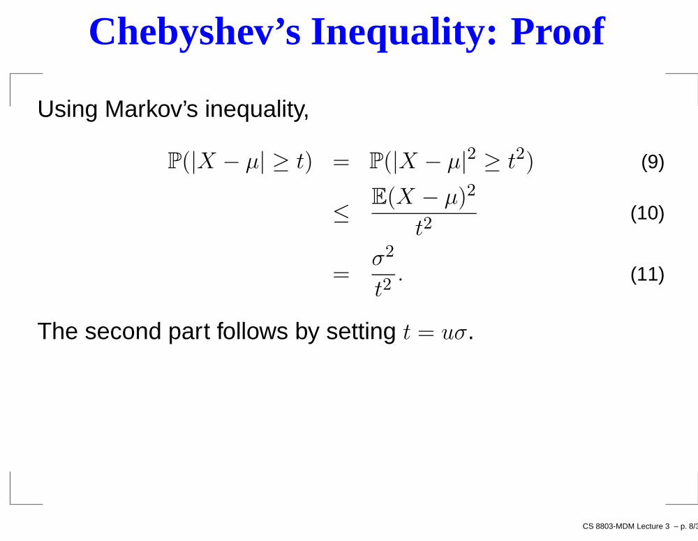
Chebyshev’s Inequality: Proof

Using Markov’s inequality,

P(|X − µ| ≥ t) = P(|X − µ|2 ≥ t2) (9)

≤ E(X − µ)2

t2(10)

=σ2

t2. (11)

The second part follows by setting t = uσ.

CS 8803-MDM Lecture 3 – p. 8/32

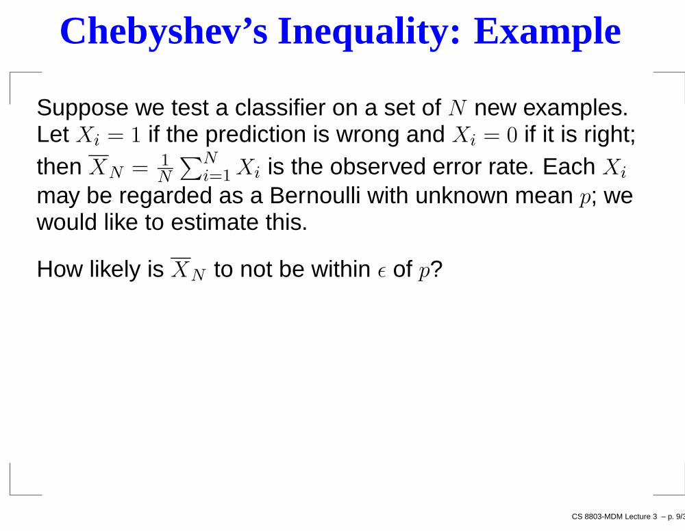
Chebyshev’s Inequality: Example

Suppose we test a classifier on a set of N new examples.Let Xi = 1 if the prediction is wrong and Xi = 0 if it is right;then XN = 1N

∑Ni=1 Xi is the observed error rate. Each Xi

may be regarded as a Bernoulli with unknown mean p; wewould like to estimate this.

How likely is XN to not be within ǫ of p?

CS 8803-MDM Lecture 3 – p. 9/32

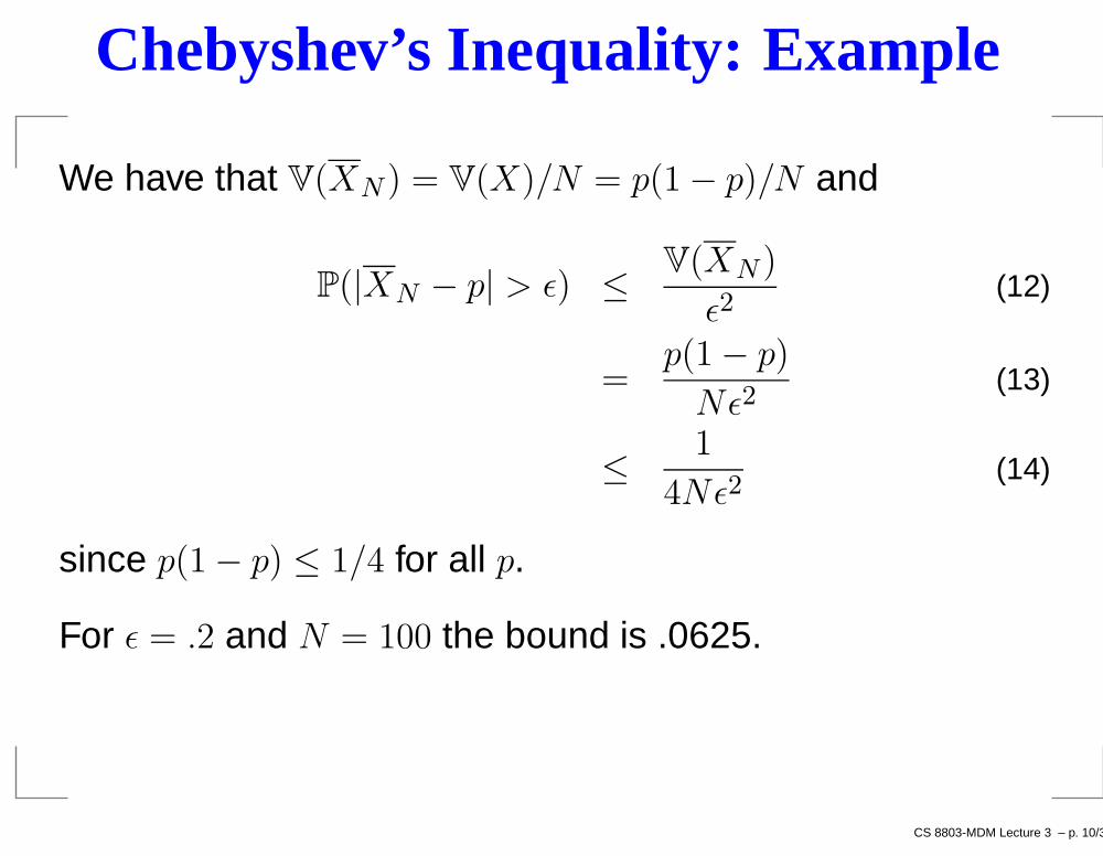
Chebyshev’s Inequality: Example

We have that V(XN ) = V(X)/N = p(1 − p)/N and

P(|XN − p| > ǫ) ≤V(XN )

ǫ2(12)

=p(1 − p)

Nǫ2(13)

≤ 14Nǫ2

(14)

since p(1 − p) ≤ 1/4 for all p.

For ǫ = .2 and N = 100 the bound is .0625.

CS 8803-MDM Lecture 3 – p. 10/32

Asymptotic theory

What happens as you get more data.

CS 8803-MDM Lecture 3 – p. 14/32

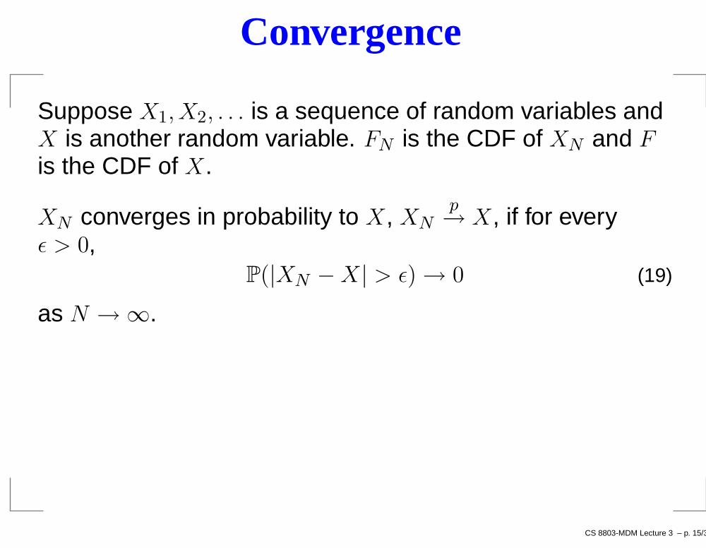
Convergence

Suppose X1, X2, . . . is a sequence of random variables andX is another random variable. FN is the CDF of XN and Fis the CDF of X.

XN converges in probability to X, XNp→ X, if for every

ǫ > 0,P(|XN − X| > ǫ) → 0 (19)

as N → ∞.

CS 8803-MDM Lecture 3 – p. 15/32

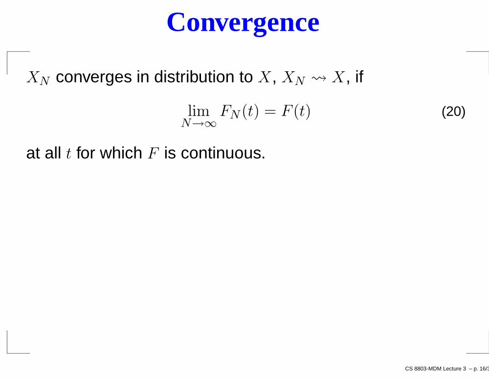
Convergence

XN converges in distribution to X, XN X, if

limN→∞

FN (t) = F (t) (20)

at all t for which F is continuous.

CS 8803-MDM Lecture 3 – p. 16/32

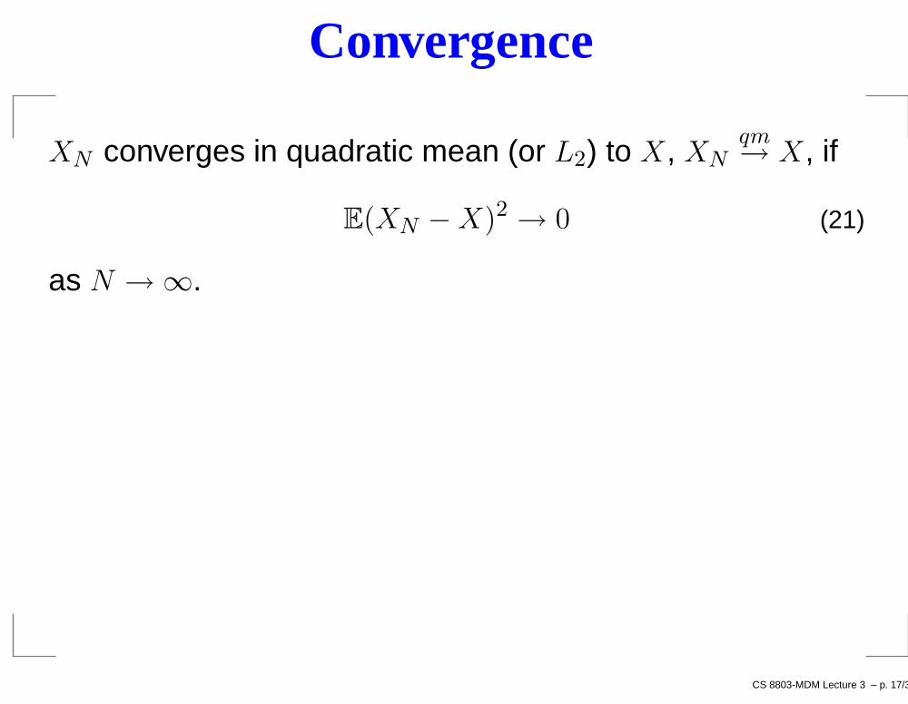
Convergence

XN converges in quadratic mean (or L2) to X, XNqm→ X, if

E(XN − X)2 → 0 (21)

as N → ∞.

CS 8803-MDM Lecture 3 – p. 17/32

Convergence

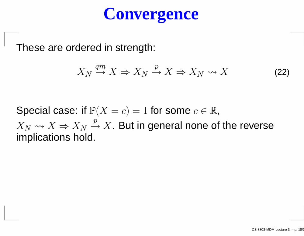
These are ordered in strength:

XNqm→ X ⇒ XN

p→ X ⇒ XN X (22)

Special case: if P(X = c) = 1 for some c ∈ R,XN X ⇒ XN

p→ X. But in general none of the reverseimplications hold.

CS 8803-MDM Lecture 3 – p. 18/32

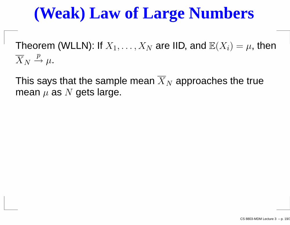
(Weak) Law of Large Numbers

Theorem (WLLN): If X1, . . . , XN are IID, and E(Xi) = µ, then

XNp→ µ.

This says that the sample mean XN approaches the truemean µ as N gets large.

CS 8803-MDM Lecture 3 – p. 19/32

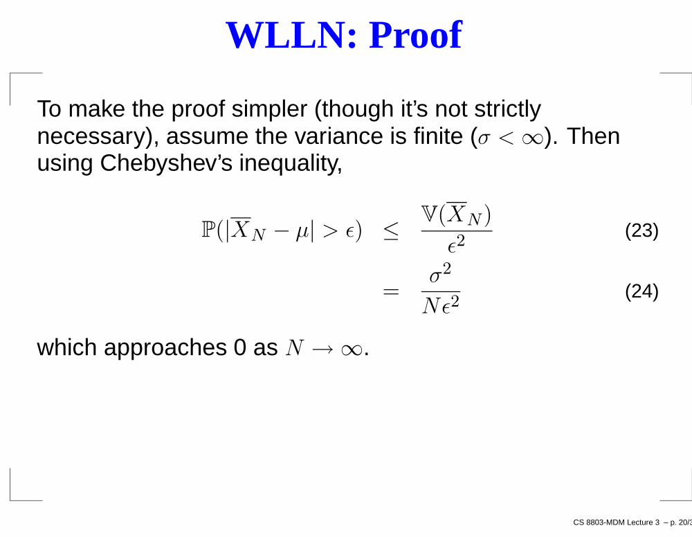
WLLN: Proof

To make the proof simpler (though it’s not strictlynecessary), assume the variance is finite (σ < ∞). Thenusing Chebyshev’s inequality,

P(|XN − µ| > ǫ) ≤V(XN )

ǫ2(23)

=σ2

Nǫ2(24)

which approaches 0 as N → ∞.

CS 8803-MDM Lecture 3 – p. 20/32

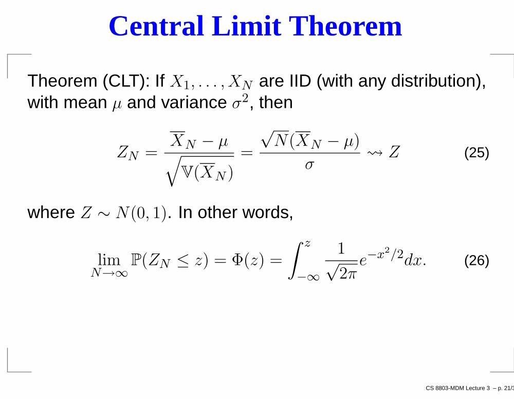
Central Limit Theorem

Theorem (CLT): If X1, . . . , XN are IID (with any distribution),with mean µ and variance σ2, then

ZN =XN − µ√

V(XN )=

√N(XN − µ)

σ Z (25)

where Z ∼ N(0, 1). In other words,

limN→∞

P(ZN ≤ z) = Φ(z) =∫ z

−∞

1√2π

e−x2/2dx. (26)

CS 8803-MDM Lecture 3 – p. 21/32

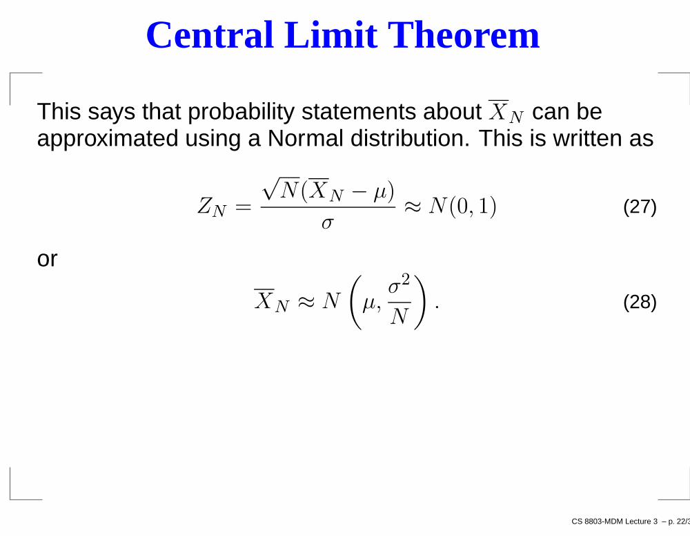
Central Limit Theorem

This says that probability statements about XN can beapproximated using a Normal distribution. This is written as

ZN =

√N(XN − µ)

σ≈ N(0, 1) (27)

or

XN ≈ N(

µ,σ2

N

). (28)

CS 8803-MDM Lecture 3 – p. 22/32

Acknowledgement: The slides are from Alexander Gray @ George Tech.

Welcome to This CourseToday A Dataset Types of Estimation Problems Density Estimation Density Estimation Density Estimation Regression Regression Classification Classification Types of Data Models Error (Loss Function)

Learning and Prediction Some Questions What is Machine Learning? Inference What is Machine Learning? History of Machine Learning History of Machine Learning Growth of Machine Learning Goals of This Course Review of Syllabus Review of Syllabus Review of Syllabus Review of Syllabus Books Hidden Messages of This Course Grading Survey/Comparisons How Hard Will This Course Be? 3_stat2.pdfToday Standard Normal Distribution Markov's Inequality Markov's Inequality: Proof Chebyshev's Inequality Chebyshev's Inequality: Proof Chebyshev's Inequality: Example Chebyshev's Inequality: Example Hoeffding's Inequality Hoeffding's Inequality Hoeffding's Inequality: Example Convergence Convergence Convergence Convergence (Weak)Law of Large Numbers WLLN: Proof Central Limit Theorem Central Limit Theorem Point estimation Sampling distribution Properties of Estimators Asymptotic Normality

3_stat2.pdfCourse StuffToday Samples Spaces and Events Probability Random Variables Distribution Functions Distribution Functions Discrete Distributions Continuous Distributions Multivariate Distributions Marginal Distributions Conditional Distributions Bayes' Rule Independence Expectation Variance Sample Statistics