


γλώσσες
Σελίδες
Νομικός

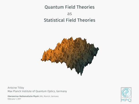
Quantum Field Theoriesas
Statistical Field Theories
Antoine TilloyMax Planck Institute of Quantum Optics, Germany
Oberseminar Mathematische Physik LMU, Munich, GermanyFebruary 1, 2017

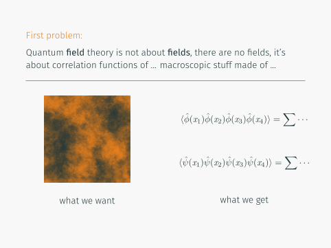
First problem:
Quantum field theory is not about fields, there are no fields, it’sabout correlation functions of ... macroscopic stuff made of ...
⟨ϕ(x1)ϕ(x2)ϕ(x3)ϕ(x4)⟩ =∑
· · ·
⟨ψ(x1)ψ(x2)ψ(x3)ψ(x4)⟩ =∑
· · ·
what we want what we get
First problem:
Quantum field theory is not about fields, there are no fields, it’sabout correlation functions of ... macroscopic stuff made of ...
⟨ϕ(x1)ϕ(x2)ϕ(x3)ϕ(x4)⟩ =∑
· · ·
⟨ψ(x1)ψ(x2)ψ(x3)ψ(x4)⟩ =∑
· · ·
what we want what we get

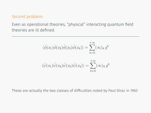
Second problem:
Even as operational theories, “physical” interacting quantum fieldtheories are ill defined.
⟨ϕ(x1)ϕ(x2)ϕ(x3)ϕ(x4)⟩ =+∞∑k=0
(∞)k gk
⟨ψ(x1)ψ(x2)ψ(x3)ψ(x4)⟩ =+∞∑k=0
(∞)k gk
These are actually the two classes of difficulties noted by Paul Dirac in 1963
Second problem:
Even as operational theories, “physical” interacting quantum fieldtheories are ill defined.
⟨ϕ(x1)ϕ(x2)ϕ(x3)ϕ(x4)⟩ =+∞∑k=0
(∞)k gk
⟨ψ(x1)ψ(x2)ψ(x3)ψ(x4)⟩ =+∞∑k=0
(∞)k gk
These are actually the two classes of difficulties noted by Paul Dirac in 1963
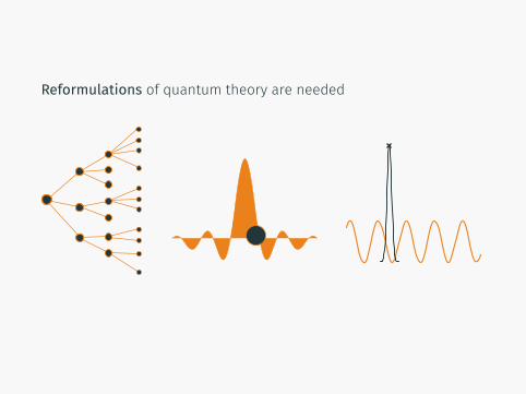
Reformulations of quantum theory are needed

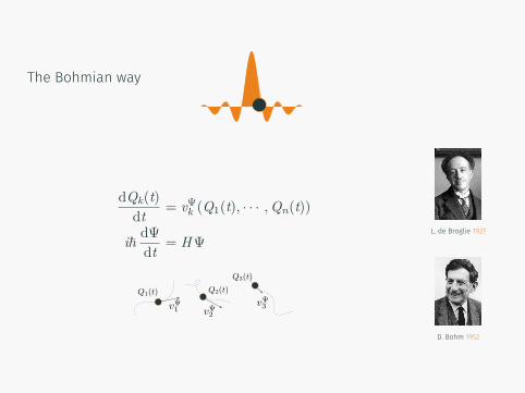
The Bohmian way
dQk(t)dt = vΨk (Q1(t), · · · ,Qn(t))
iℏ dΨdt = HΨ
L. de Broglie 1927
D. Bohm 1952
The Bohmian way
dQk(t)dt = vΨk (Q1(t), · · · ,Qn(t))
iℏ dΨdt = HΨ
L. de Broglie 1927
D. Bohm 1952

Subtleties
Lorentz invariance
Either fixed foliation of foliation determined by the wave function →the letter but not the spirit
Particle creation-annihilation 2 solutions
∙ Stochastic creation-annihilation events∙ Resurrect the Dirac sea

Subtleties
Lorentz invariance
Either fixed foliation of foliation determined by the wave function →the letter but not the spirit
Particle creation-annihilation 2 solutions
∙ Stochastic creation-annihilation events∙ Resurrect the Dirac sea

Subtleties
Lorentz invariance
Either fixed foliation of foliation determined by the wave function →the letter but not the spirit
Particle creation-annihilation
2 solutions
∙ Stochastic creation-annihilation events∙ Resurrect the Dirac sea

Subtleties
Lorentz invariance
Either fixed foliation of foliation determined by the wave function →the letter but not the spirit
Particle creation-annihilation 2 solutions
∙ Stochastic creation-annihilation events∙ Resurrect the Dirac sea
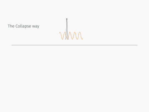
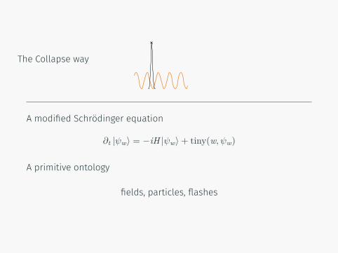
The Collapse way
A modified Schrödinger equation
∂t |ψw⟩ = −iH |ψw⟩+ tiny(w, ψw)
A primitive ontology
fields, particles, flashes
The Collapse way
A modified Schrödinger equation
∂t |ψw⟩ = −iH |ψw⟩+ tiny(w, ψw)
A primitive ontology
fields, particles, flashes

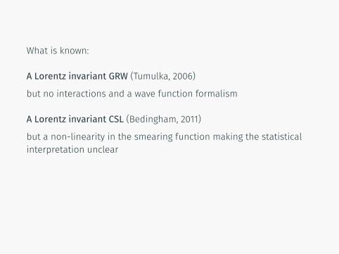
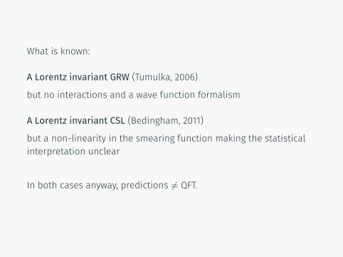
What is known:
A Lorentz invariant GRW (Tumulka, 2006)
but no interactions and a wave function formalism
A Lorentz invariant CSL (Bedingham, 2011)
but a non-linearity in the smearing function making the statisticalinterpretation unclear
In both cases anyway, predictions = QFT.

What is known:
A Lorentz invariant GRW (Tumulka, 2006)
but no interactions and a wave function formalism
A Lorentz invariant CSL (Bedingham, 2011)
but a non-linearity in the smearing function making the statisticalinterpretation unclear
In both cases anyway, predictions = QFT.
What is known:
A Lorentz invariant GRW (Tumulka, 2006)
but no interactions and a wave function formalism
A Lorentz invariant CSL (Bedingham, 2011)
but a non-linearity in the smearing function making the statisticalinterpretation unclear
In both cases anyway, predictions = QFT.
What is known:
A Lorentz invariant GRW (Tumulka, 2006)
but no interactions and a wave function formalism
A Lorentz invariant CSL (Bedingham, 2011)
but a non-linearity in the smearing function making the statisticalinterpretation unclear
In both cases anyway, predictions = QFT.
Objective:
Construct a relativistic collapse model, naturally written as aLorentz invariant statistical field theory, that can be embeddedwithin an “orthodox” interacting quantum field theory.
In provocative form
1. Collapse models can be made equivalent to quantum theory2. Quantum field theories can be written as statistical field
theories3. The two previous points are equivalent
Objective:
Construct a relativistic collapse model, naturally written as aLorentz invariant statistical field theory, that can be embeddedwithin an “orthodox” interacting quantum field theory.
In provocative form
1. Collapse models can be made equivalent to quantum theory
2. Quantum field theories can be written as statistical fieldtheories
3. The two previous points are equivalent
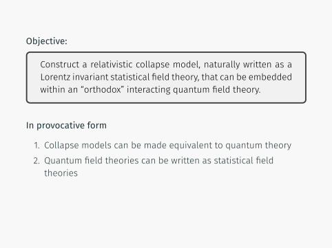
Objective:
Construct a relativistic collapse model, naturally written as aLorentz invariant statistical field theory, that can be embeddedwithin an “orthodox” interacting quantum field theory.
In provocative form
1. Collapse models can be made equivalent to quantum theory2. Quantum field theories can be written as statistical field
theories
3. The two previous points are equivalent
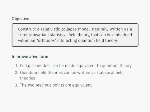
Objective:
Construct a relativistic collapse model, naturally written as aLorentz invariant statistical field theory, that can be embeddedwithin an “orthodox” interacting quantum field theory.
In provocative form
1. Collapse models can be made equivalent to quantum theory2. Quantum field theories can be written as statistical field
theories3. The two previous points are equivalent
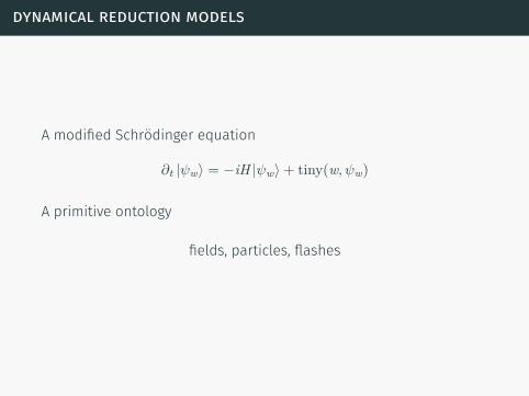
dynamical reduction models
A modified Schrödinger equation
∂t |ψw⟩ = −iH |ψw⟩+ tiny(w, ψw)
A primitive ontology
fields, particles, flashes
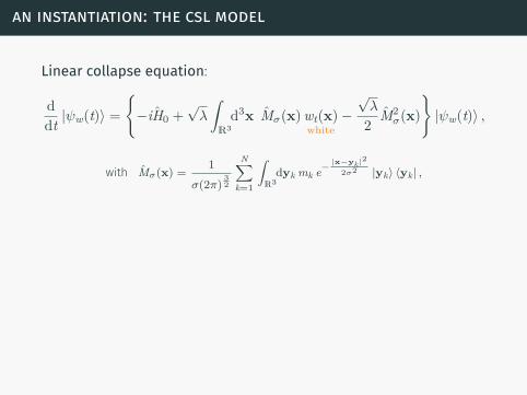
an instantiation: the csl model
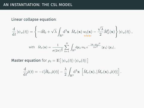
Linear collapse equation:
ddt |ψw(t)⟩ =
−iH0 +
√λ
∫R3
d3x Mσ(x)wt(x)white
−√λ
2 M2σ(x)
|ψw(t)⟩ ,
with Mσ(x) =1
σ(2π)32
N∑k=1
∫R3
dyk mk e−|x−yk|
2
2σ2 |yk⟩ ⟨yk| ,
Master equation for ρt = E[|ψw(t)⟩ ⟨ψw(t)|
]ddt ρ(t) = −i [H0, ρ(t)]−
λ
2
∫R3
d3x[Mσ(x), [Mσ(x), ρ(t)]
].
More generally ρt = Φt · ρ0with Φ linear Completely Positive Trace Preserving
needs to be an “unraveling” of a nice open-system evolution
Gisin Diosi
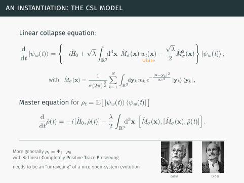
an instantiation: the csl model
Linear collapse equation:
ddt |ψw(t)⟩ =
−iH0 +
√λ
∫R3
d3x Mσ(x)wt(x)white
−√λ
2 M2σ(x)
|ψw(t)⟩ ,
with Mσ(x) =1
σ(2π)32
N∑k=1
∫R3
dyk mk e−|x−yk|
2
2σ2 |yk⟩ ⟨yk| ,
Master equation for ρt = E[|ψw(t)⟩ ⟨ψw(t)|
]ddt ρ(t) = −i [H0, ρ(t)]−
λ
2
∫R3
d3x[Mσ(x), [Mσ(x), ρ(t)]
].
More generally ρt = Φt · ρ0with Φ linear Completely Positive Trace Preserving
needs to be an “unraveling” of a nice open-system evolution
Gisin Diosi
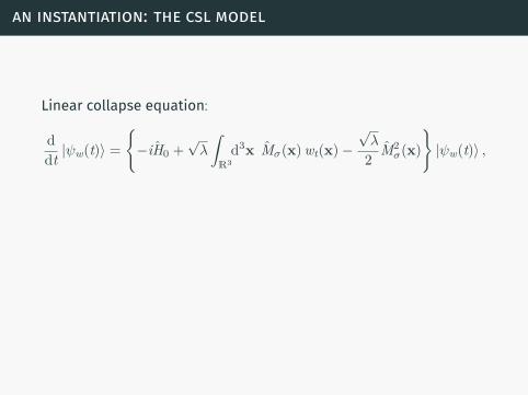
an instantiation: the csl model
Linear collapse equation:
ddt |ψw(t)⟩ =
−iH0 +
√λ
∫R3
d3x Mσ(x)wt(x)white
−√λ
2 M2σ(x)
|ψw(t)⟩ ,
with Mσ(x) =1
σ(2π)32
N∑k=1
∫R3
dyk mk e−|x−yk|
2
2σ2 |yk⟩ ⟨yk| ,
Master equation for ρt = E[|ψw(t)⟩ ⟨ψw(t)|
]ddt ρ(t) = −i [H0, ρ(t)]−
λ
2
∫R3
d3x[Mσ(x), [Mσ(x), ρ(t)]
].
More generally ρt = Φt · ρ0with Φ linear Completely Positive Trace Preserving
needs to be an “unraveling” of a nice open-system evolution
Gisin Diosi
an instantiation: the csl model
Linear collapse equation:
ddt |ψw(t)⟩ =
−iH0 +
√λ
∫R3
d3x Mσ(x)wt(x)−√λ
2 M2σ(x)
|ψw(t)⟩ ,
Normalization and cooking:
∣∣∣ψw(t)⟩=
|ψw(t)⟩√⟨ψw(t)|ψw(t)⟩
dµt(w) = ⟨ψw(t)|ψw(t)⟩ · dµ0(w)
wt(x) = 2√λ ⟨Mσ(x)⟩+ bt(x)
white.
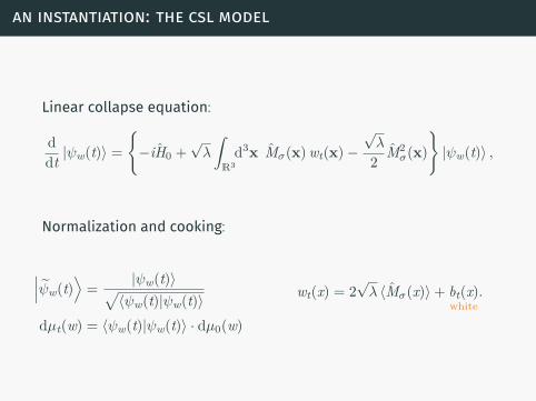
an instantiation: the csl model
Linear collapse equation:
ddt |ψw(t)⟩ =
−iH0 +
√λ
∫R3
d3x Mσ(x)wt(x)−√λ
2 M2σ(x)
|ψw(t)⟩ ,
Normalization and cooking:
∣∣∣ψw(t)⟩=
|ψw(t)⟩√⟨ψw(t)|ψw(t)⟩
dµt(w) = ⟨ψw(t)|ψw(t)⟩ · dµ0(w)
wt(x) = 2√λ ⟨Mσ(x)⟩+ bt(x)
white.

an instantiation: the csl model
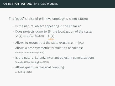
The “good” choice of primitive ontology is w, not ⟨M(x)⟩:
∙ Is the natural object appearing in the linear eq.∙ Does projects down to R3 the localization of the state:
wt(x) = 2√λ ⟨Mσ(x)⟩+ bt(x)
white
∙ Allows to reconstruct the state exactly: w → |ψw⟩∙ Allows a time symmetric formulation of collapse
Bedingham & Maroney (2015)
∙ Is the natural Lorentz invariant object in generalizationsTumulka (2006), Bedingham (2011)
∙ Allows quantum classical couplingAT & Diósi (2016)

an instantiation: the csl model
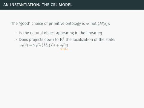
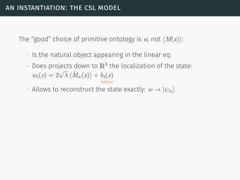
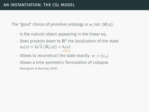
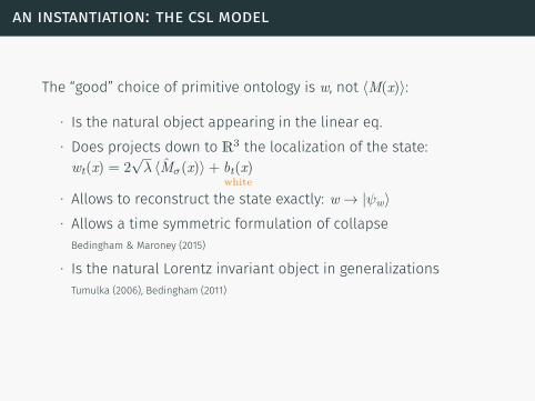
The “good” choice of primitive ontology is w, not ⟨M(x)⟩:
∙ Is the natural object appearing in the linear eq.
∙ Does projects down to R3 the localization of the state:wt(x) = 2
√λ ⟨Mσ(x)⟩+ bt(x)
white
∙ Allows to reconstruct the state exactly: w → |ψw⟩∙ Allows a time symmetric formulation of collapse
Bedingham & Maroney (2015)
∙ Is the natural Lorentz invariant object in generalizationsTumulka (2006), Bedingham (2011)
∙ Allows quantum classical couplingAT & Diósi (2016)
an instantiation: the csl model
The “good” choice of primitive ontology is w, not ⟨M(x)⟩:
∙ Is the natural object appearing in the linear eq.∙ Does projects down to R3 the localization of the state:
wt(x) = 2√λ ⟨Mσ(x)⟩+ bt(x)
white
∙ Allows to reconstruct the state exactly: w → |ψw⟩∙ Allows a time symmetric formulation of collapse
Bedingham & Maroney (2015)
∙ Is the natural Lorentz invariant object in generalizationsTumulka (2006), Bedingham (2011)
∙ Allows quantum classical couplingAT & Diósi (2016)
an instantiation: the csl model
The “good” choice of primitive ontology is w, not ⟨M(x)⟩:
∙ Is the natural object appearing in the linear eq.∙ Does projects down to R3 the localization of the state:
wt(x) = 2√λ ⟨Mσ(x)⟩+ bt(x)
white
∙ Allows to reconstruct the state exactly: w → |ψw⟩
∙ Allows a time symmetric formulation of collapseBedingham & Maroney (2015)
∙ Is the natural Lorentz invariant object in generalizationsTumulka (2006), Bedingham (2011)
∙ Allows quantum classical couplingAT & Diósi (2016)
an instantiation: the csl model
The “good” choice of primitive ontology is w, not ⟨M(x)⟩:
∙ Is the natural object appearing in the linear eq.∙ Does projects down to R3 the localization of the state:
wt(x) = 2√λ ⟨Mσ(x)⟩+ bt(x)
white
∙ Allows to reconstruct the state exactly: w → |ψw⟩∙ Allows a time symmetric formulation of collapse
Bedingham & Maroney (2015)
∙ Is the natural Lorentz invariant object in generalizationsTumulka (2006), Bedingham (2011)
∙ Allows quantum classical couplingAT & Diósi (2016)
an instantiation: the csl model
The “good” choice of primitive ontology is w, not ⟨M(x)⟩:
∙ Is the natural object appearing in the linear eq.∙ Does projects down to R3 the localization of the state:
wt(x) = 2√λ ⟨Mσ(x)⟩+ bt(x)
white
∙ Allows to reconstruct the state exactly: w → |ψw⟩∙ Allows a time symmetric formulation of collapse
Bedingham & Maroney (2015)
∙ Is the natural Lorentz invariant object in generalizationsTumulka (2006), Bedingham (2011)
∙ Allows quantum classical couplingAT & Diósi (2016)
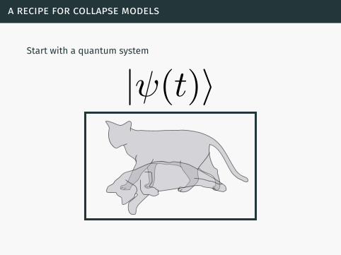
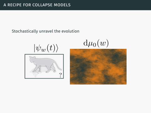
a recipe for collapse models
Start with a quantum system
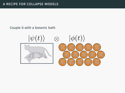
a recipe for collapse models
Couple it with a bosonic bath
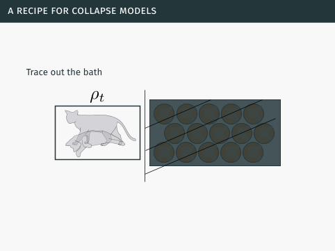
a recipe for collapse models
Trace out the bath
a recipe for collapse models
Stochastically unravel the evolution
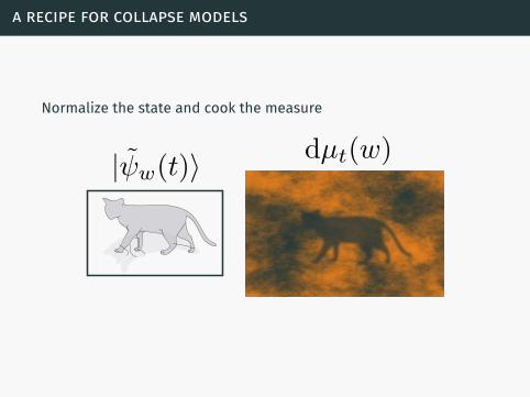
a recipe for collapse models
Normalize the state and cook the measure

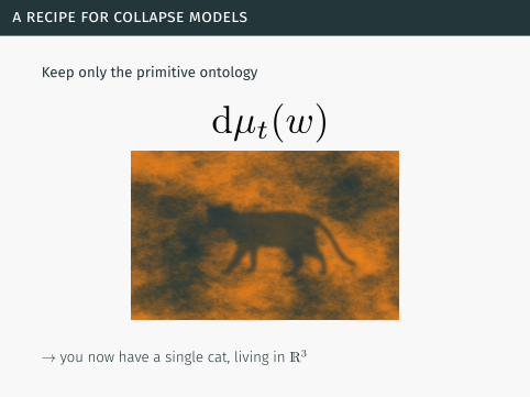
a recipe for collapse models
Keep only the primitive ontology
→ you now have a single cat, living in R3
a recipe for collapse models
Keep only the primitive ontology
→ you now have a single cat, living in R3

changing the recipe for qft
Take an interacting QFT:
changing the recipe for qft
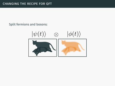
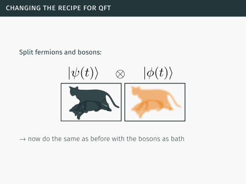
Split fermions and bosons:
→ now do the same as before with the bosons as bath
changing the recipe for qft
Split fermions and bosons:
→ now do the same as before with the bosons as bath
changing the recipe for qft
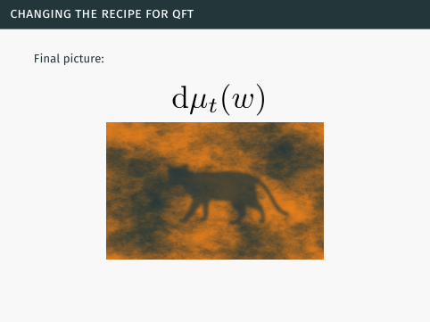
Final picture:
This time without changing the empirical content of the theory!

changing the recipe for qft
Final picture:
This time without changing the empirical content of the theory!
in practice
Consider a Yukawa theory:
Lf(ψ, ∂µψ) = ψ(i/∂ − mf)ψ
Lint(ψ, ϕ) = g ψ ψ ϕ
Lb(ϕ, ∂µϕ) =12∂µϕ∂
µϕ− 12m2
bϕ2,
Take the momentum regularization Λ as fundamental
in practice
Consider a Yukawa theory:
Lf(ψ, ∂µψ) = ψ(i/∂ − mf)ψ
Lint(ψ, ϕ) = g ψ ψ ϕ
Lb(ϕ, ∂µϕ) =12∂µϕ∂
µϕ− 12m2
bϕ2,
Take the momentum regularization Λ as fundamental

in practice
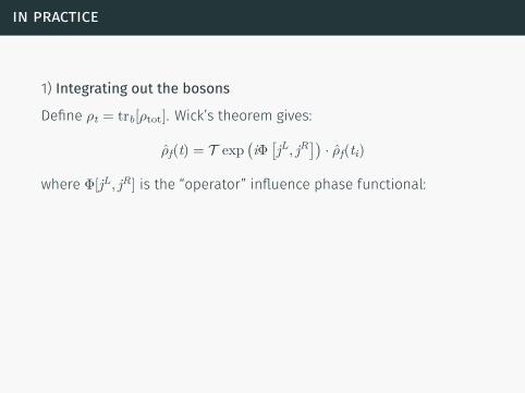
1) Integrating out the bosons
Define ρt = trb[ρtot].
Wick’s theorem gives:
ρf(t) = T exp(iΦ
[jL, jR
])· ρf(ti)
where Φ[jL, jR] is the “operator” influence phase functional:
iΦ[jL, jR
]=
∫ t
ti
∫ t
ti
d4x d4y D(x, y) jL(x)jR(y)
− 12θ(x
0 − y0)D(x, y) jL(x)jL(y)− 12θ(y
0 − x0)D(x, y) jR(x)jR(y)
with D(x, y) = trb
[ϕ(x)ϕ(y) ρb(ti)
].
in practice
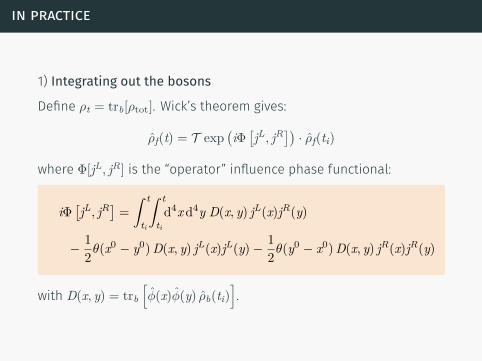
1) Integrating out the bosons
Define ρt = trb[ρtot]. Wick’s theorem gives:
ρf(t) = T exp(iΦ
[jL, jR
])· ρf(ti)
where Φ[jL, jR] is the “operator” influence phase functional:
iΦ[jL, jR
]=
∫ t
ti
∫ t
ti
d4x d4y D(x, y) jL(x)jR(y)
− 12θ(x
0 − y0)D(x, y) jL(x)jL(y)− 12θ(y
0 − x0)D(x, y) jR(x)jR(y)
with D(x, y) = trb
[ϕ(x)ϕ(y) ρb(ti)
].
in practice
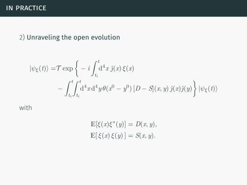
2) Unraveling the open evolution
|ψξ(t)⟩ =T exp− i
∫ t
ti
d4x ȷ(x) ξ(x)
−∫ t
ti
∫ t
ti
d4x d4y θ(x0 − y0) [D − S](x, y) ȷ(x)ȷ(y)|ψξ(t)⟩
with
E[ξ(x)ξ∗(y)] = D(x, y),E[ ξ(x) ξ(y) ] = S(x, y).
Note: importantly, finding ξ with the correlation matrix D is alwayspossible (the relation matrix S is a free parameter)
in practice
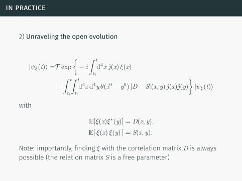
2) Unraveling the open evolution
|ψξ(t)⟩ =T exp− i
∫ t
ti
d4x ȷ(x) ξ(x)
−∫ t
ti
∫ t
ti
d4x d4y θ(x0 − y0) [D − S](x, y) ȷ(x)ȷ(y)|ψξ(t)⟩
with
E[ξ(x)ξ∗(y)] = D(x, y),E[ ξ(x) ξ(y) ] = S(x, y).
Note: importantly, finding ξ with the correlation matrix D is alwayspossible (the relation matrix S is a free parameter)

in practice
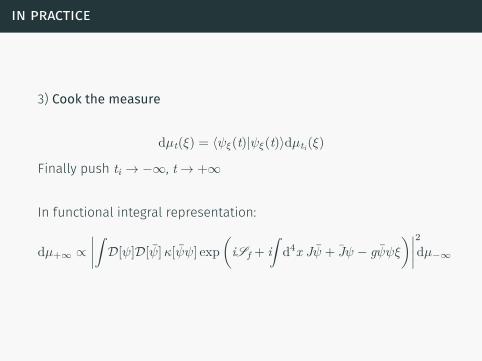
3) Cook the measure
dµt(ξ) = ⟨ψξ(t)|ψξ(t)⟩dµti(ξ)
Finally push ti → −∞, t → +∞
In functional integral representation:
dµ+∞ ∝∣∣∣∣∫ D[ψ]D[ψ]κ[ψψ] exp
(iSf + i
∫d4x Jψ + Jψ − gψψξ
)∣∣∣∣2dµ−∞

in practice
3) Cook the measure
dµt(ξ) = ⟨ψξ(t)|ψξ(t)⟩dµti(ξ)
Finally push ti → −∞, t → +∞
In functional integral representation:
dµ+∞ ∝∣∣∣∣∫ D[ψ]D[ψ]κ[ψψ] exp
(iSf + i
∫d4x Jψ + Jψ − gψψξ
)∣∣∣∣2dµ−∞
in practice
3) Cook the measure
dµt(ξ) = ⟨ψξ(t)|ψξ(t)⟩dµti(ξ)
Finally push ti → −∞, t → +∞
In functional integral representation:
dµ+∞ ∝∣∣∣∣∫ D[ψ]D[ψ]κ[ψψ] exp
(iSf + i
∫d4x Jψ + Jψ − gψψξ
)∣∣∣∣2dµ−∞

in practice
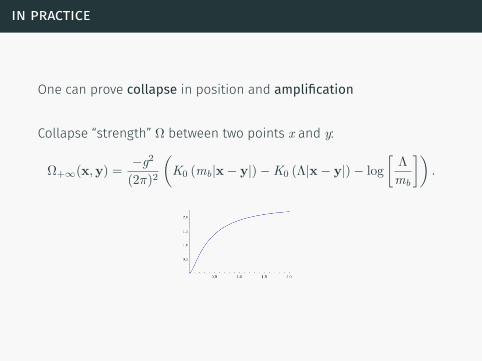
One can prove collapse in position and amplification
Collapse “strength” Ω between two points x and y:
Ω+∞(x,y) = −g2
(2π)2
(K0 (mb|x − y|)− K0 (Λ|x − y|)− log
[Λ
mb
]).
in practice
One can prove collapse in position and amplification
Collapse “strength” Ω between two points x and y:
Ω+∞(x,y) = −g2
(2π)2
(K0 (mb|x − y|)− K0 (Λ|x − y|)− log
[Λ
mb
]).

discussion

reconsidering collapse
∙ Collapse can be seen as an interpretation of QFT∙ Expected empirical signatures of collapse computed so far areartifacts of Markovianity / frame dependence.

reconsidering collapse
∙ Collapse can be seen as an interpretation of QFT
∙ Expected empirical signatures of collapse computed so far areartifacts of Markovianity / frame dependence.

reconsidering collapse
∙ Collapse can be seen as an interpretation of QFT∙ Expected empirical signatures of collapse computed so far areartifacts of Markovianity / frame dependence.

reconsidering qft
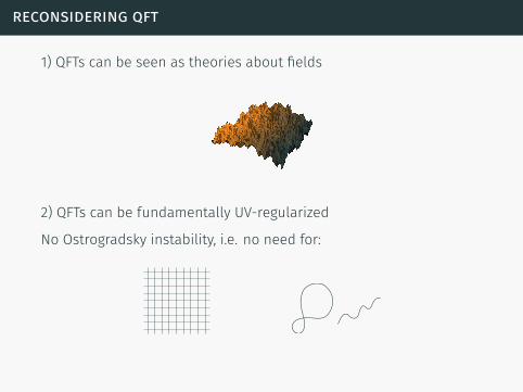
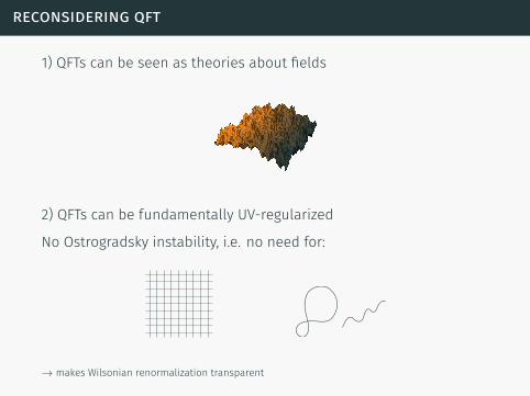
1) QFTs can be seen as theories about fields
2) QFTs can be fundamentally UV-regularized
No Ostrogradsky instability, i.e. no need for:
→ makes Wilsonian renormalization transparent
reconsidering qft
1) QFTs can be seen as theories about fields
2) QFTs can be fundamentally UV-regularized
No Ostrogradsky instability, i.e. no need for:
→ makes Wilsonian renormalization transparent
reconsidering qft
1) QFTs can be seen as theories about fields
2) QFTs can be fundamentally UV-regularized
No Ostrogradsky instability, i.e. no need for:
→ makes Wilsonian renormalization transparent
reconsidering qft
1) QFTs can be seen as theories about fields
2) QFTs can be fundamentally UV-regularized
No Ostrogradsky instability, i.e. no need for:
→ makes Wilsonian renormalization transparent
reconsidering qft
1) QFTs can be seen as theories about fields
2) QFTs can be fundamentally UV-regularized
No Ostrogradsky instability, i.e. no need for:
→ makes Wilsonian renormalization transparent

limitations
∙ So far, harder to analyse with QED
∙ Not trivial to connect with physical parameters →renormalization
∙ It would be better to work from first principles

limitations
∙ So far, harder to analyse with QED∙ Not trivial to connect with physical parameters →renormalization
∙ It would be better to work from first principles

limitations
∙ So far, harder to analyse with QED∙ Not trivial to connect with physical parameters →renormalization
∙ It would be better to work from first principles

Summary
One can construct “simple” relativistic collapse models
They can be made equivalent to QFT
This gives an interpretation of QFT as a SFT
Still analytical, numerical and conceptual cleaning to do

Summary
One can construct “simple” relativistic collapse models
They can be made equivalent to QFT
This gives an interpretation of QFT as a SFT
Still analytical, numerical and conceptual cleaning to do

Summary
One can construct “simple” relativistic collapse models
They can be made equivalent to QFT
This gives an interpretation of QFT as a SFT
Still analytical, numerical and conceptual cleaning to do

Summary
One can construct “simple” relativistic collapse models
They can be made equivalent to QFT
This gives an interpretation of QFT as a SFT
Still analytical, numerical and conceptual cleaning to do

Summary
One can construct “simple” relativistic collapse models
They can be made equivalent to QFT
This gives an interpretation of QFT as a SFT
Still analytical, numerical and conceptual cleaning to do
Top Related