

γλώσσες
Σελίδες
Νομικός

Harrod –Domar Growth Model
Solow Growth Model
Endogenous Growth Model
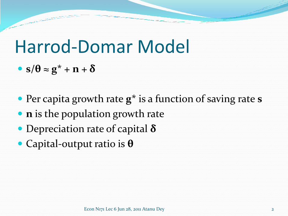
Harrod-Domar Model s/θ ≈ g* + n + δ
Per capita growth rate g* is a function of saving rate s
n is the population growth rate
Depreciation rate of capital δ
Capital-output ratio is θ
Econ N171 Lec 6 Jun 28, 2011 Atanu Dey 2
Robert Solow (b. 1924)
Got the Nobel prize in economics 1987
Sveriges Riksbank Prize in Economic Sciences in Memory of Alfred Nobel
Added labor and technology to the H-D model
Econ N171 Lec 6 Jun 28, 2011 Atanu Dey 3

Wit & Wisdom of Bob Solow Everything reminds Milton Friedman of the money supply.
Everything reminds me of sex, but I try to keep it out of my papers.
Over the long term, places with strong, distinctive identities are more likely to prosper than places without them. Every place must identify its strongest most distinctive features and develop them or run the risk of being all things to all persons and nothing special to any...Livability is not a middle-class luxury. It is an economic imperative."
"There is no evidence that God ever intended the United States of America to have a higher per capita income than the rest of the world for eternity."[
Econ N171 Lec 6 Jun 28, 2011 Atanu Dey 4
Extension to the Harrod-Domar model
Solow extended the Harrod-Domar model by
Adding labor as a factor of production
Requiring diminishing returns to labor and capital separately, and constant returns to scale for both factors combined
Introducing a time-varying technology variable distinct from capital and labor
The capital-output and capital-labor ratios are not fixed as they are in the Harrod-Domar model.
Econ N171 Lec 6 Jun 28, 2011 Atanu Dey 5
What it says
Economies will conditionally converge to the same level of income if they have the same rates of savings, depreciation, labor force growth and development
It provides the basic framework for the study of convergence across countries
Econ N171 Lec 6 Jun 28, 2011 Atanu Dey 6
Production function
Relates production (output, or income) to factors (or inputs
Y = F(K, L)
Graph a production function with diminishing returns to K
Cobb-Douglas Production function
Y = AK**(1-α)L**α
Each factor has diminishing returns
Both combined are constant returns to scale
Econ N171 Lec 6 Jun 28, 2011 Atanu Dey 7
Constant Returns to Scale Y = F(K, L)
If you multiply each factor by λ, then the output also goes up by λ
Do this for the Cobb-Douglas production function
Econ N171 Lec 6 Jun 28, 2011 Atanu Dey 8
Output as a function of capital Per capita output y and per capita capital k
Y = F(K,L)
Divide both sides by L
Y/L = F(K/L, 1)
y = f(k)
Plot output y as a function of k, noting that there’s diminishing returns to capital
Econ N171 Lec 6 Jun 28, 2011 Atanu Dey 9
Solow Growth Model Capital stock grows every period
K(t+1) = (1 – δ)K(t) + S(t)
If population grows at rate n, then per capita capital stock k grows at?
Note P(t + 1) = (1 + n)P(t)
k(t) = K(t)/P(t) and k(t + 1) = K(t + 1)/P(t + 1)
Rearranging : (1 + n)k(t + 1) = (1 – δ)k(t) + sy(t)
RHS is depreciated per capita capital and current per capita savings
LHS is new per capita capital – modified by the population growth rate
Econ N171 Lec 6 Jun 28, 2011 Atanu Dey 10
Alternate Form Δk = sf(k) – (δ + n)k
Capital-labor ratio k = K/L
Shows that the growth of k depends on the savings sf(k), after allowing for the amount of capital required to serving depreciation, δk, and after providing the existing amount of capital per worker to net new workers joining the labor force, nk
Econ N171 Lec 6 Jun 28, 2011 Atanu Dey 11
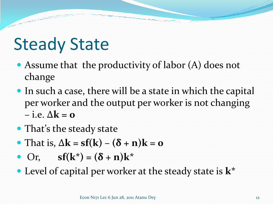
Steady State Assume that the productivity of labor (A) does not
change
In such a case, there will be a state in which the capital per worker and the output per worker is not changing – i.e. Δk = 0
That’s the steady state
That is, Δk = sf(k) – (δ + n)k = 0
Or, sf(k*) = (δ + n)k*
Level of capital per worker at the steady state is k*
Econ N171 Lec 6 Jun 28, 2011 Atanu Dey 12
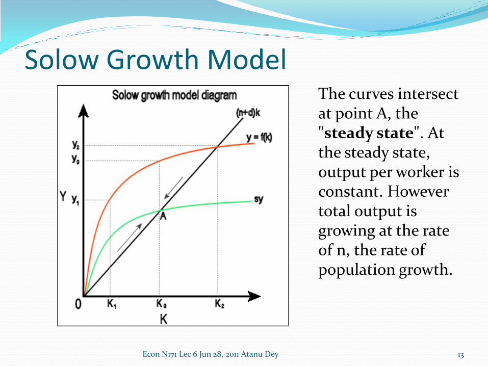
Solow Growth ModelThe curves intersect at point A, the "steady state". At the steady state, output per worker is constant. However total output is growing at the rate of n, the rate of population growth.
13Econ N171 Lec 6 Jun 28, 2011 Atanu Dey
Solow Growth Model (2)
Econ N171 Lec 6 Jun 28, 2011 Atanu Dey 14
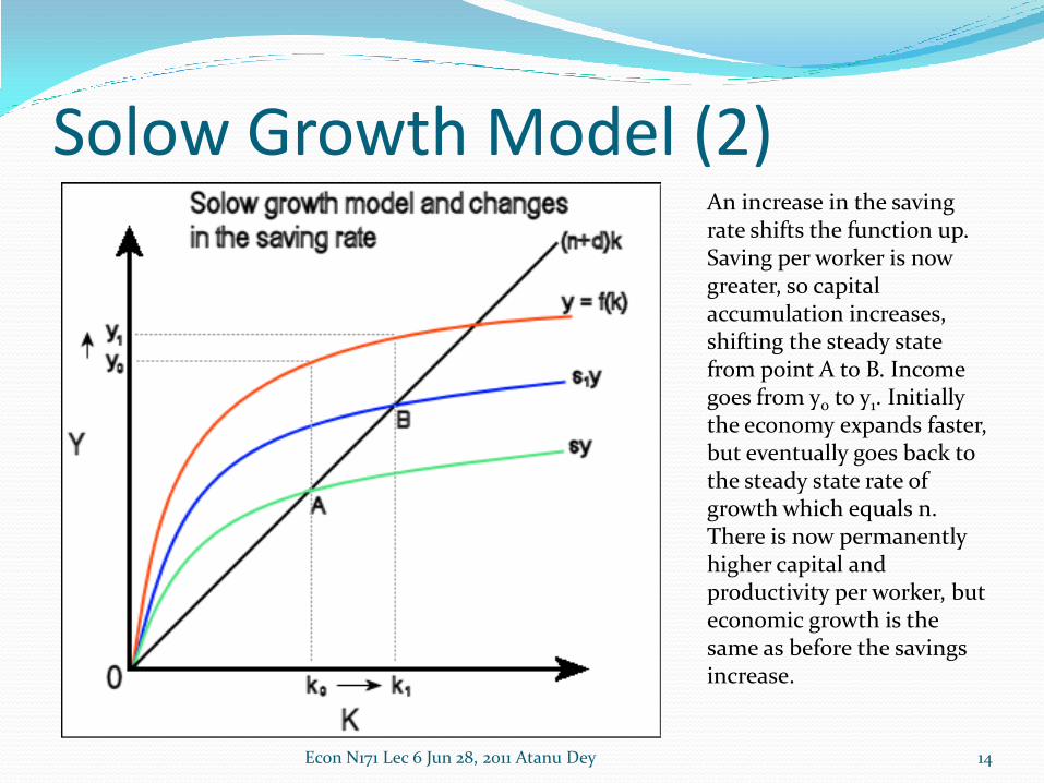
An increase in the saving rate shifts the function up. Saving per worker is now greater, so capital accumulation increases, shifting the steady state from point A to B. Income goes from y0 to y1. Initially the economy expands faster, but eventually goes back to the steady state rate of growth which equals n.There is now permanently higher capital and productivity per worker, but economic growth is the same as before the savings increase.
Solow Growth Model (3)
Econ N171 Lec 6 Jun 28, 2011 Atanu Dey 15
Short-run Implications Policy measures like tax cuts or investment subsidies can
affect the steady state level of output but not the long-run growth rate.
Growth is affected only in the short-run as the economy converges to the new steady state output level.
The rate of growth as the economy converges to the steady state is determined by the rate of capital accumulation
Capital accumulation is in turn determined by the savings rate (the proportion of output used to create more capital rather than being consumed) and the rate of capital depreciation
Econ N171 Lec 6 Jun 28, 2011 Atanu Dey 16
Long-run Implications The long-run rate of growth is exogenously –
determined outside of the model
Predicts that an economy will always converge towards a steady state rate of growth, which depends only on the rate of technological progress and the rate of labor force growth.
A country with a higher saving rate will experience faster growth, e.g. Singapore had a 40% saving rate in the period 1960 to 1996 and annual GDP growth of 5-6%, compared with Kenya in the same time period which had a 15% saving rate and annual GDP growth of just 1%.
Econ N171 Lec 6 Jun 28, 2011 Atanu Dey 17
Top Related