Phase-field simulations ofcrystal growth

Mathis Plapp

Laboratoire de Physique de la Matière CondenséeCNRS/Ecole Polytechnique, 91128 Palaiseau, France

Solidification microstructures

Dendrites (Co-Cr)

Hexagonal cells (Sn-Pb)

Eutectic colonies Peritectic composite (Fe-Ni)

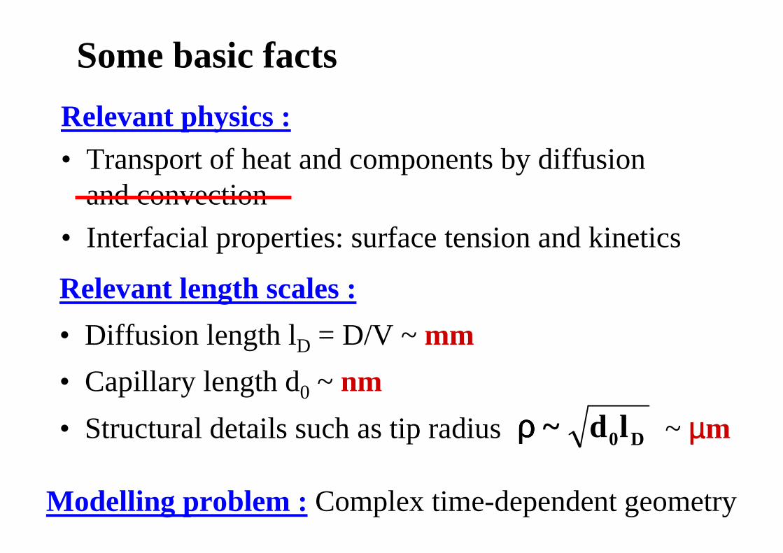
Some basic facts

Relevant physics :• Transport of heat and components by diffusion

and convection

• Interfacial properties: surface tension and kinetics

D0ld~ρρρρ

Modelling problem : Complex time-dependent geometry

Relevant length scales :

• Diffusion length lD = D/V ~ mm

• Capillary length d0 ~ nm

• Structural details such as tip radius ~ µµµµm

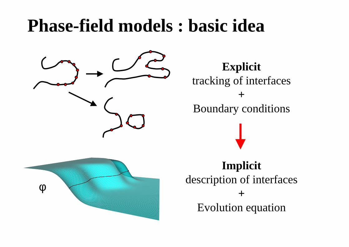
Phase-field models : basic idea

Explicittracking of interfaces

+Boundary conditions

Implicitdescription of interfaces

+Evolution equation

φ

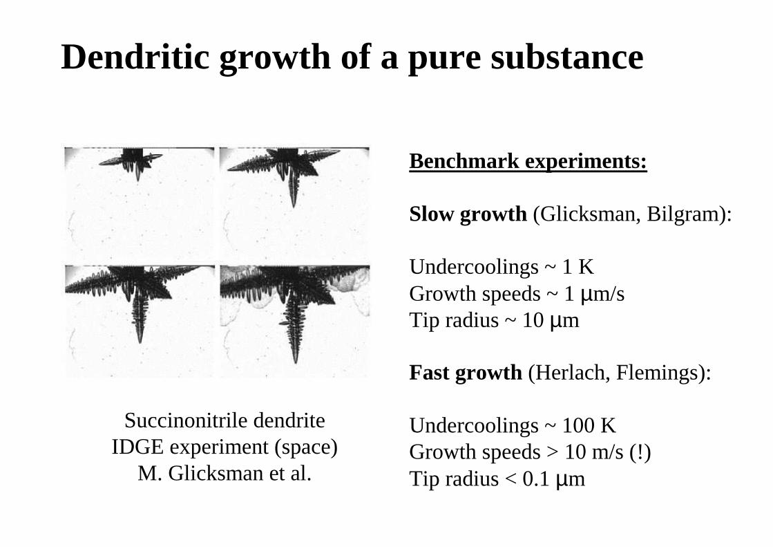
Dendritic growth of a pure substance

Benchmark experiments:

Slow growth (Glicksman, Bilgram):

Undercoolings ~ 1 KGrowth speeds ~ 1 µm/sTip radius ~ 10 µm

Fast growth (Herlach, Flemings):

Undercoolings ~ 100 KGrowth speeds > 10 m/s (!)Tip radius < 0.1 µm

Succinonitrile dendriteIDGE experiment (space)

M. Glicksman et al.

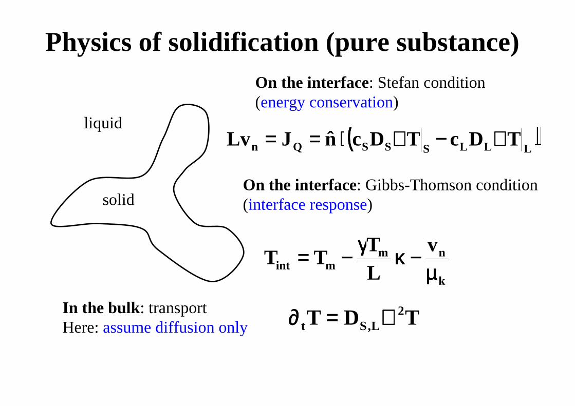
Physics of solidification (pure substance)

solid

liquid

In the bulk : transportHere: assume diffusion only TDT 2

L,St ∇∇∇∇====∂∂∂∂

(((( ))))LLLSSSQn TDcTDcnJLv ∇∇∇∇−−−−∇∇∇∇⋅⋅⋅⋅========

On the interface: Stefan condition(energy conservation)

On the interface: Gibbs-Thomson condition(interface response)

k

nmmint

vLT

TTµµµµ

−−−−κκκκγγγγ−−−−====

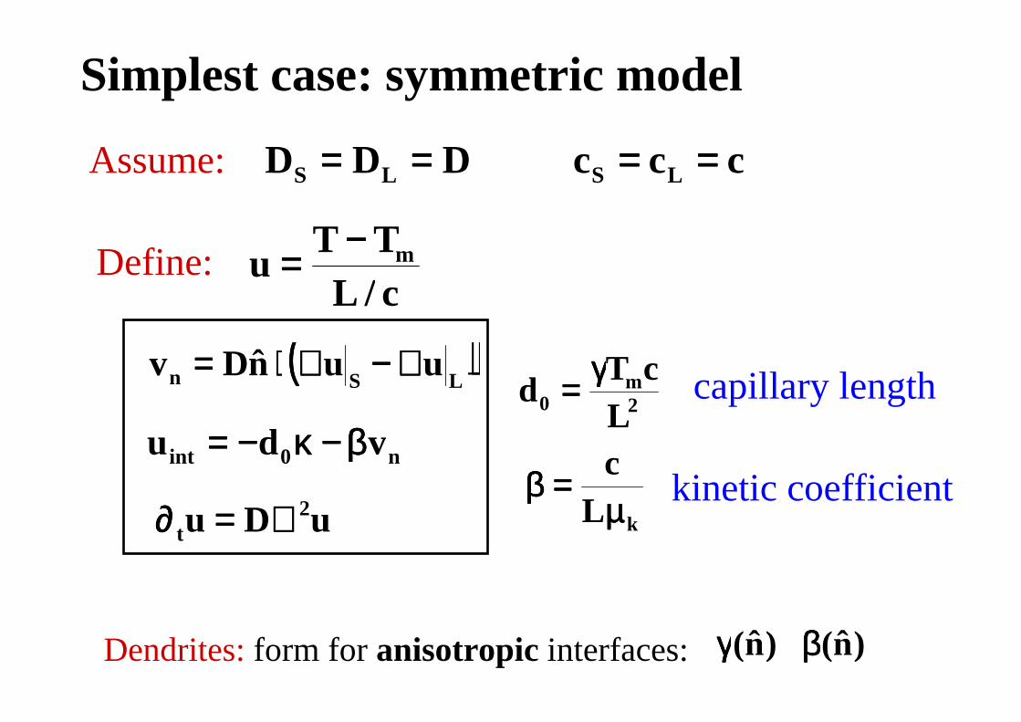
Simplest case: symmetric model

uDu 2t ∇∇∇∇====∂∂∂∂

(((( ))))LSn uunDv ∇∇∇∇−−−−∇∇∇∇⋅⋅⋅⋅====

Assume:

n0int vdu ββββ−−−−κκκκ−−−−====

Define:c/LTT

u m−−−−====

DDD LS ======== ccc LS ========

capillary length2m

0 LcT

dγγγγ====

)n(ββββ

kinetic coefficient

Dendrites: form for anisotropic interfaces: )n(γγγγ

kLcµµµµ

====ββββ

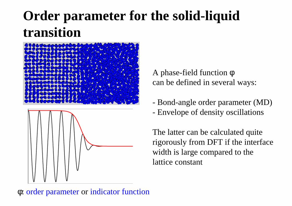
Order parameter for the solid-liquidtransition

φ: order parameteror indicator function

A phase-field functionφcan be defined in several ways:

- Bond-angle order parameter (MD)- Envelope of density oscillations

The latter can be calculated quiterigorously from DFT if the interfacewidth is large compared to thelattice constant

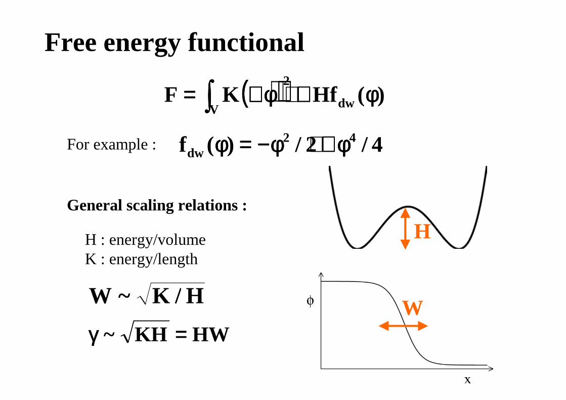
Free energy functional

(((( )))) )(HfKF dw

2

Vφφφφ++++φφφφ∇∇∇∇==== ∫∫∫∫4/2/)(f 42

dw φφφφ++++φφφφ−−−−====φφφφ

H : energy/volumeK : energy/length

H/K~W

HWKH~ ====γγγγ

For example :

General scaling relations :

H

W

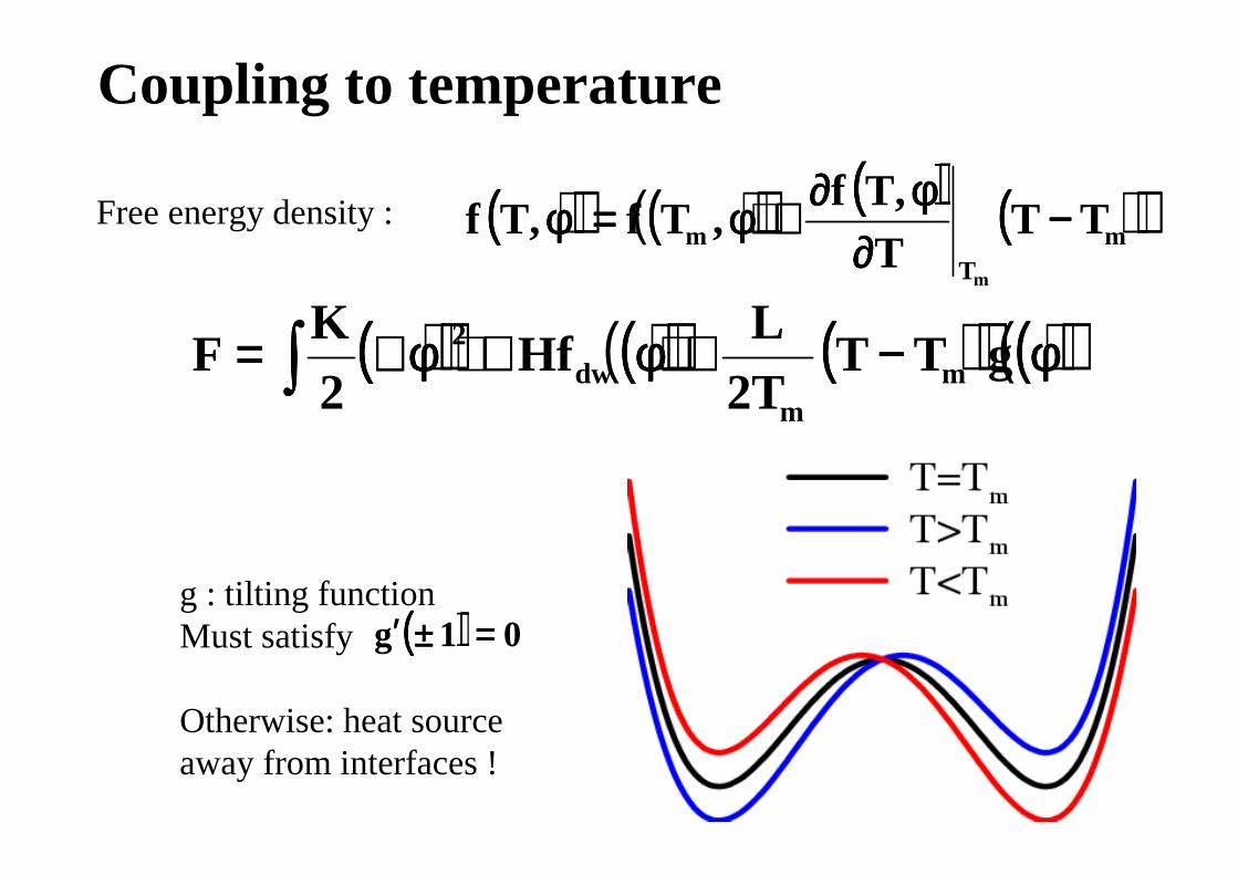
Coupling to temperature

(((( )))) (((( )))) (((( )))) (((( ))))φφφφ−−−−++++φφφφ++++φφφφ∇∇∇∇==== ∫∫∫∫ gTTT2L

Hf2K

F mm

dw2

g : tilting functionMust satisfy

Otherwise: heat sourceaway from interfaces !

(((( )))) 01g ====±±±±′′′′

Free energy density : (((( )))) (((( )))) (((( )))) (((( ))))mT

m TTT,Tf

,Tf,Tfm

−−−−∂∂∂∂

φφφφ∂∂∂∂++++φφφφ====φφφφ

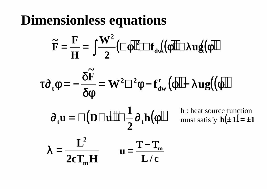
Dimensionless equations

(((( )))) (((( )))) (((( ))))φφφφλλλλ++++φφφφ++++φφφφ∇∇∇∇======== ∫∫∫∫ ugf2

WHF

F~

dw2

2

HcT2L

m

2

====λλλλ

(((( )))) (((( ))))φφφφ′′′′λλλλ−−−−φφφφ′′′′−−−−φφφφ∇∇∇∇====δφδφδφδφδδδδ−−−−====φφφφ∂∂∂∂ττττ gufWF~

dw22

t

(((( )))) (((( ))))φφφφ∂∂∂∂++++∇∇∇∇∇∇∇∇====∂∂∂∂ h21

uDu tt

c/LTT

u m−−−−====

h : heat source functionmust satisfy (((( )))) 11h ±±±±====±±±±

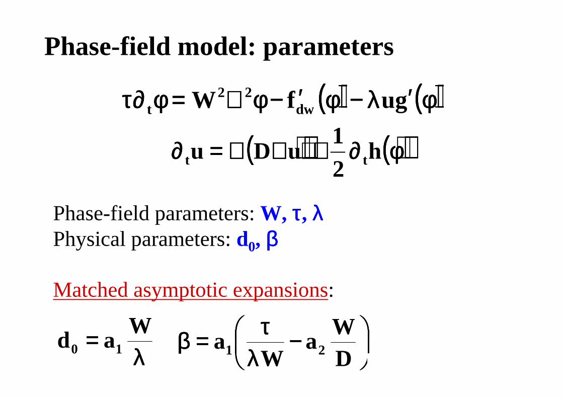
Phase-field model: parameters

Phase-field parameters: W, ττττ, λλλλPhysical parameters: d0, ββββ

Matched asymptotic expansions:

λλλλ==== W

ad 10

−−−−λλλλ

ττττ====ββββDW

aW

a 21

(((( )))) (((( ))))φφφφ′′′′λλλλ−−−−φφφφ′′′′−−−−φφφφ∇∇∇∇====φφφφ∂∂∂∂ττττ gufW dw22

t

(((( )))) (((( ))))φφφφ∂∂∂∂++++∇∇∇∇∇∇∇∇====∂∂∂∂ h21

uDu tt

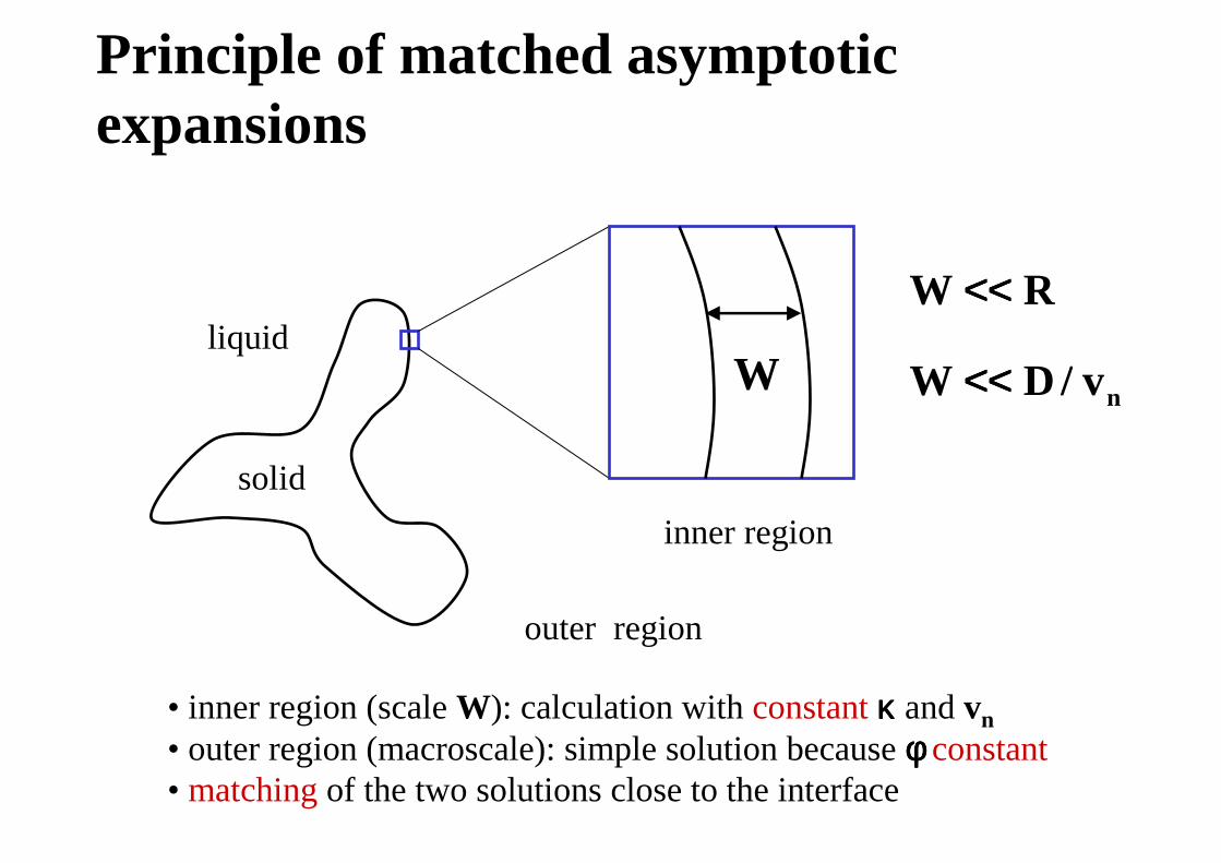
Principle of matched asymptoticexpansions

solid

liquidRW <<<<<<<<

Wnv/DW <<<<<<<<

inner region

outer region

• inner region (scaleW): calculation withconstantκκκκ andvn• outer region (macroscale): simple solution because φφφφ constant• matchingof the two solutions close to the interface

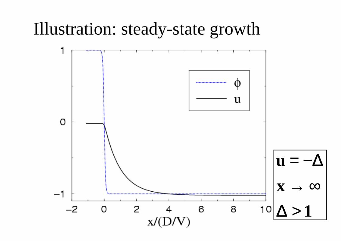
Illustration: steady-state growth

1

x

u

>∞→

−=

∆∆∆∆

∆∆∆∆

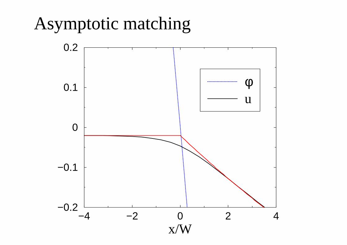
Asymptotic matching

−4 −2 0 2 4x/W

−0.2

−0.1

0

0.1

0.2

φu

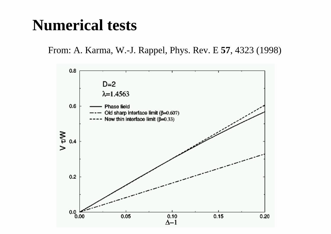
Numerical tests

From: A. Karma, W.-J. Rappel, Phys. Rev. E 57, 4323 (1998)

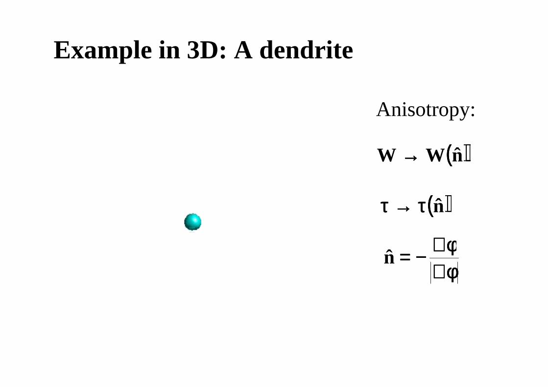
Example in 3D: A dendrite

(((( ))))nWW →→→→

Anisotropy:

φφφφ∇∇∇∇φφφφ∇∇∇∇−−−−====n

(((( ))))nττττ→→→→ττττ

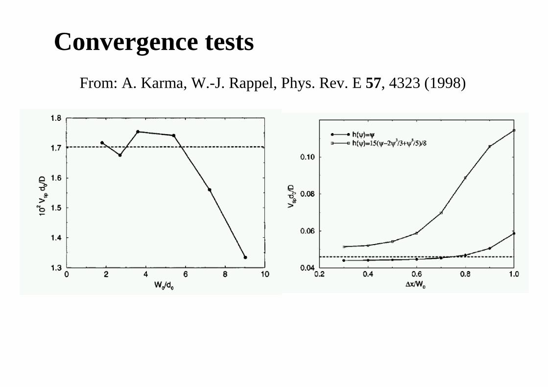
Convergence tests

From: A. Karma, W.-J. Rappel, Phys. Rev. E 57, 4323 (1998)

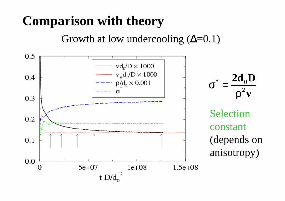
Comparison with theoryGrowth at low undercooling (∆∆∆∆=0.1)

vDd2

20*

ρρρρ====σσσσ

Selectionconstant(depends onanisotropy)

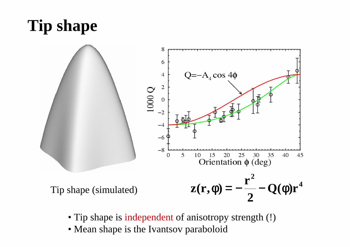
Tip shape

Tip shape (simulated)4

2

r)(Q2r

),r(z φφφφ−−−−−−−−====φφφφ

• Tip shape isindependentof anisotropy strength (!)• Mean shape is the Ivantsov paraboloid

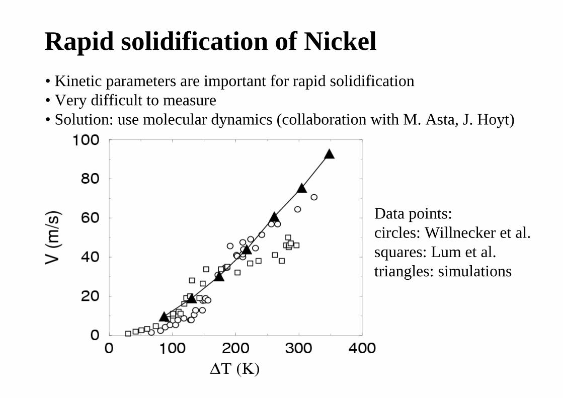
Rapid solidification of Nickel• Kinetic parameters are important for rapid solidification• Very difficult to measure• Solution: use molecular dynamics (collaboration withM. Asta, J. Hoyt)

Data points:circles: Willnecker et al.squares: Lum et al.triangles: simulations

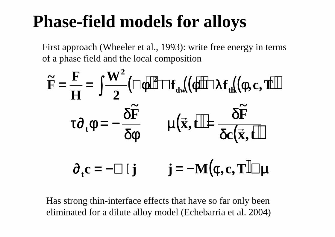
Phase-field models for alloysFirst approach (Wheeler et al., 1993): write free energy in termsof a phase field and the local composition

Has strong thin-interface effects that have so far only beeneliminated for a dilute alloy model (Echebarria et al. 2004)

(((( )))) (((( )))) (((( ))))T,c,ff2

WHF

F~

thdw2

2

φφφφλλλλ++++φφφφ++++φφφφ∇∇∇∇======== ∫∫∫∫

δφδφδφδφδδδδ−−−−====φφφφ∂∂∂∂ττττ F~

t

jct ⋅⋅⋅⋅−∇−∇−∇−∇====∂∂∂∂

(((( )))) (((( ))))t,xcF~

t,x rr

δδδδδδδδ====µµµµ

(((( )))) µµµµ∇∇∇∇φφφφ−−−−==== T,c,Mj

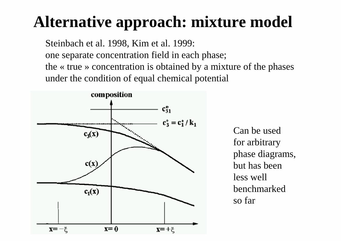
Alternative approach: mixture modelSteinbach et al. 1998, Kim et al. 1999:one separate concentration field in each phase;the « true » concentration is obtained by a mixture of thephasesunder the condition of equal chemical potential

Can be usedfor arbitraryphase diagrams, but has been less wellbenchmarkedso far

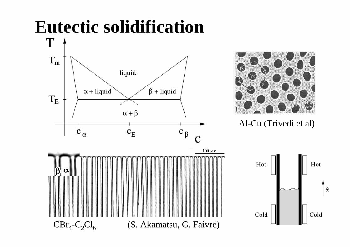
Eutectic solidification

CBr4-C2Cl6 (S. Akamatsu, G. Faivre)

Al-Cu (Trivedi et al)

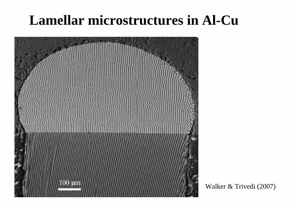
Lamellar microstructures in Al-Cu

Walker & Trivedi (2007)

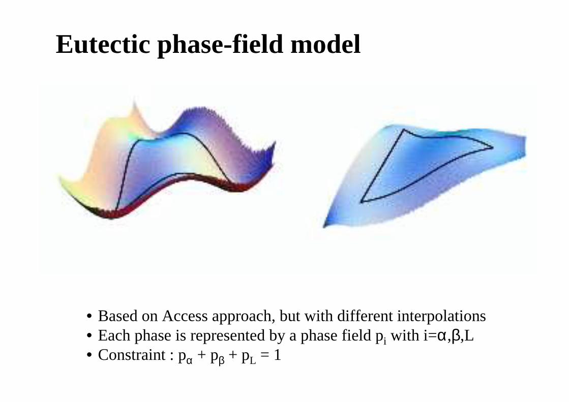
Eutectic phase-field model

• Based on Access approach, but with different interpolations• Each phase is represented by a phase field pi with i=α,β,L• Constraint : pα + pβ + pL = 1

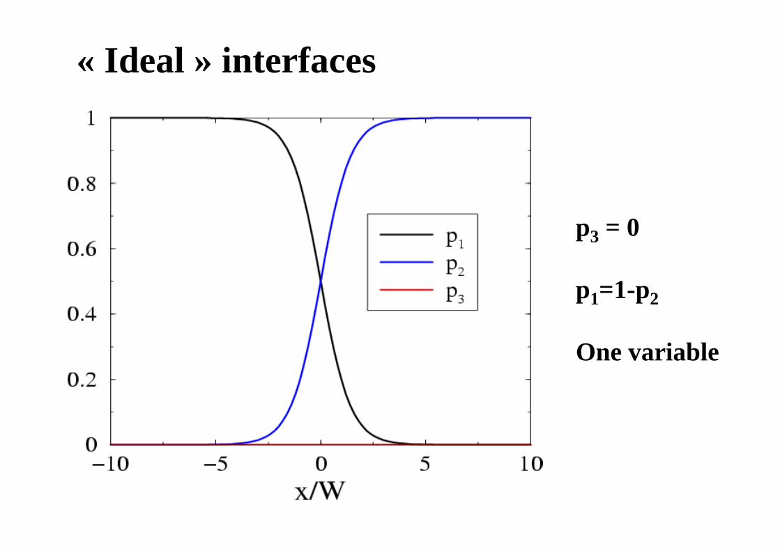
« Ideal » interfaces

p3 = 0

p1=1-p2

One variable

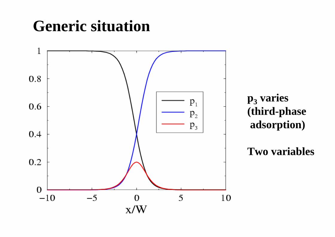
Generic situation

p3 varies(third-phaseadsorption)

Two variables

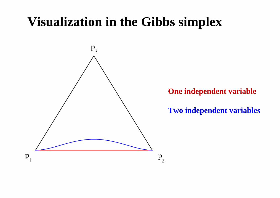
Visualization in the Gibbs simplex

One independent variable

Two independent variables

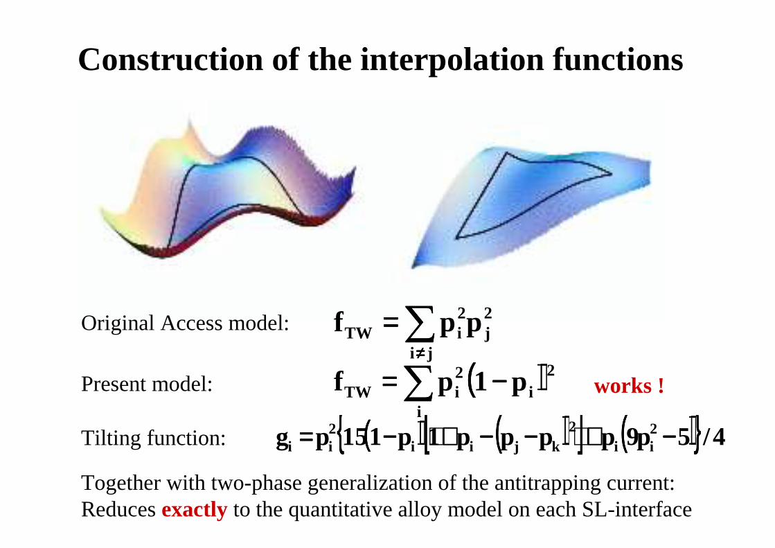
Construction of the interpolation functions

Original Access model: 2j

ji

2iTW ppf ∑∑∑∑

≠≠≠≠

====

Present model: (((( ))))2i

i

2iTW p1pf −−−−====∑∑∑∑

Tilting function: (((( )))) (((( ))))[[[[ ]]]] (((( )))) 4/5p9pppp1p115pg 2ii

2kjii

2ii −−−−++++−−−−−−−−++++−−−−====

works !

Together with two-phase generalization of the antitrapping current:Reducesexactly to the quantitative alloy model on each SL-interface

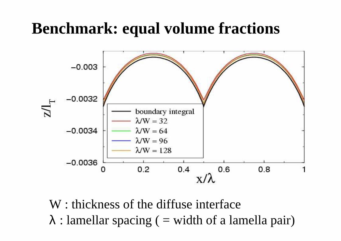
Benchmark: equal volume fractions

W : thickness of the diffuse interfaceλ : lamellar spacing ( = width of a lamella pair)

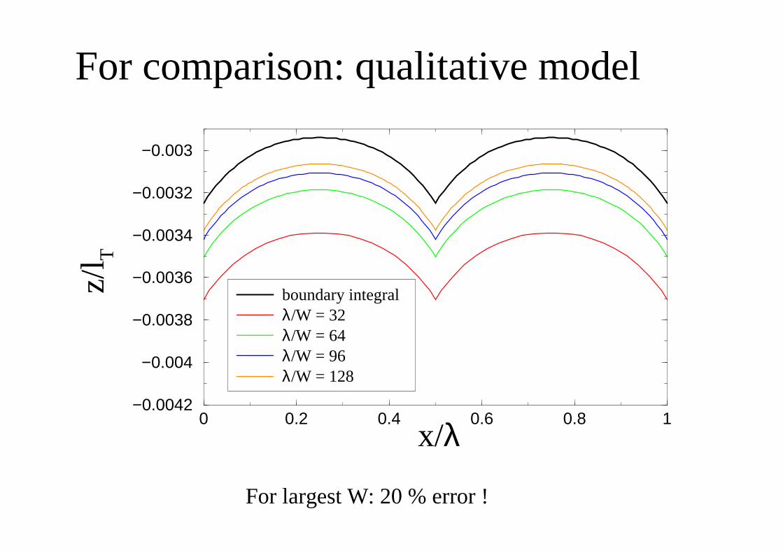
For comparison: qualitative model

0 0.2 0.4 0.6 0.8 1x/λ

−0.0042

−0.004

−0.0038

−0.0036

−0.0034

−0.0032

−0.003

z/l T

boundary integralλ/W = 32λ/W = 64λ/W = 96λ/W = 128

For largest W: 20 % error !

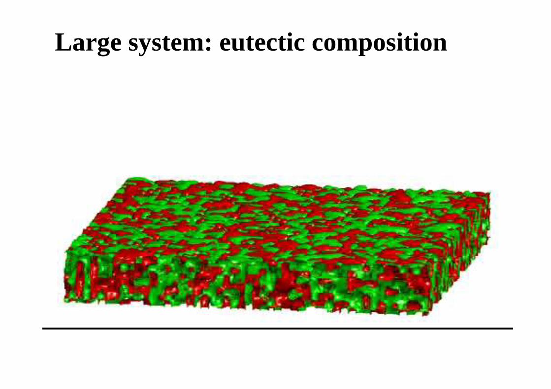
Large system: eutectic composition

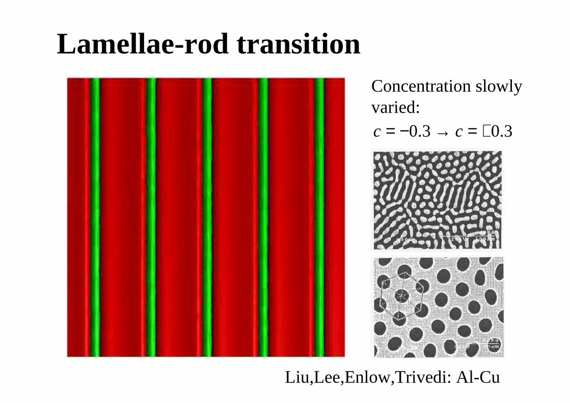
Lamellae-rod transitionConcentration slowlyvaried:

3.03.0 +=→−= cc

Liu,Lee,Enlow,Trivedi: Al-Cu

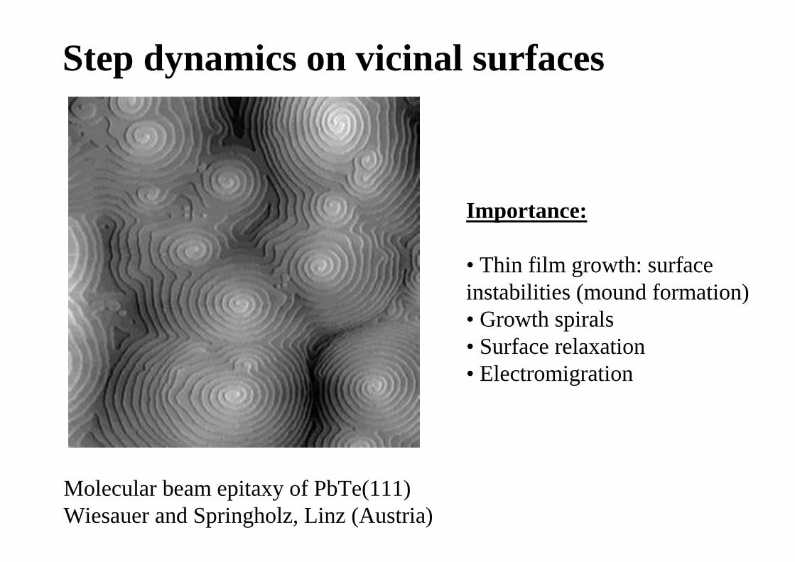
Step dynamics on vicinal surfaces

Importance:

• Thin film growth: surfaceinstabilities (mound formation)• Growth spirals• Surface relaxation• Electromigration

Molecular beam epitaxy of PbTe(111)Wiesauer and Springholz, Linz (Austria)

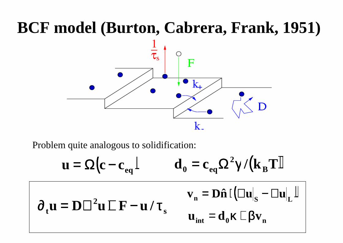
BCF model (Burton, Cabrera, Frank, 1951)

Problem quite analogous to solidification:

(((( ))))eqccu −−−−ΩΩΩΩ==== (((( ))))Tk/cd B2

eq0 γγγγΩΩΩΩ====

s2

t /uFuDu ττττ−−−−++++∇∇∇∇====∂∂∂∂(((( ))))

LSn uunDv ∇∇∇∇−−−−∇∇∇∇⋅⋅⋅⋅====

n0int vdu ββββκκκκ +=

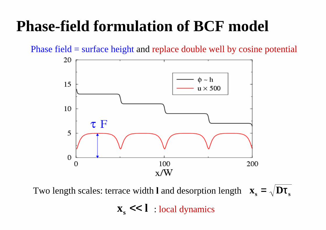
Phase-field formulation of BCF modelPhase field = surface heightand replace double well by cosine potential

ss Dx ττττ====Two length scales: terrace widthl and desorption length

lxs <<<<<<<< : local dynamics

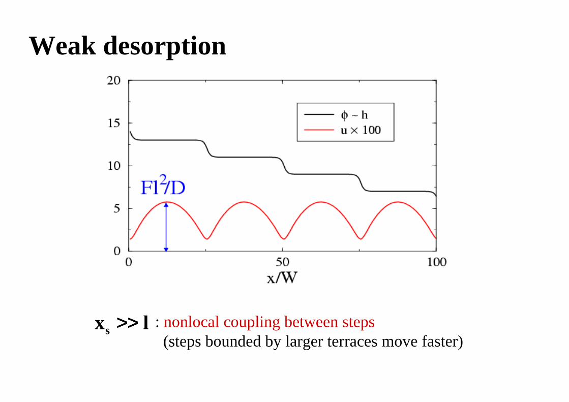
Weak desorption

lxs >>>>>>>> : nonlocal coupling between steps(steps bounded by larger terraces move faster)

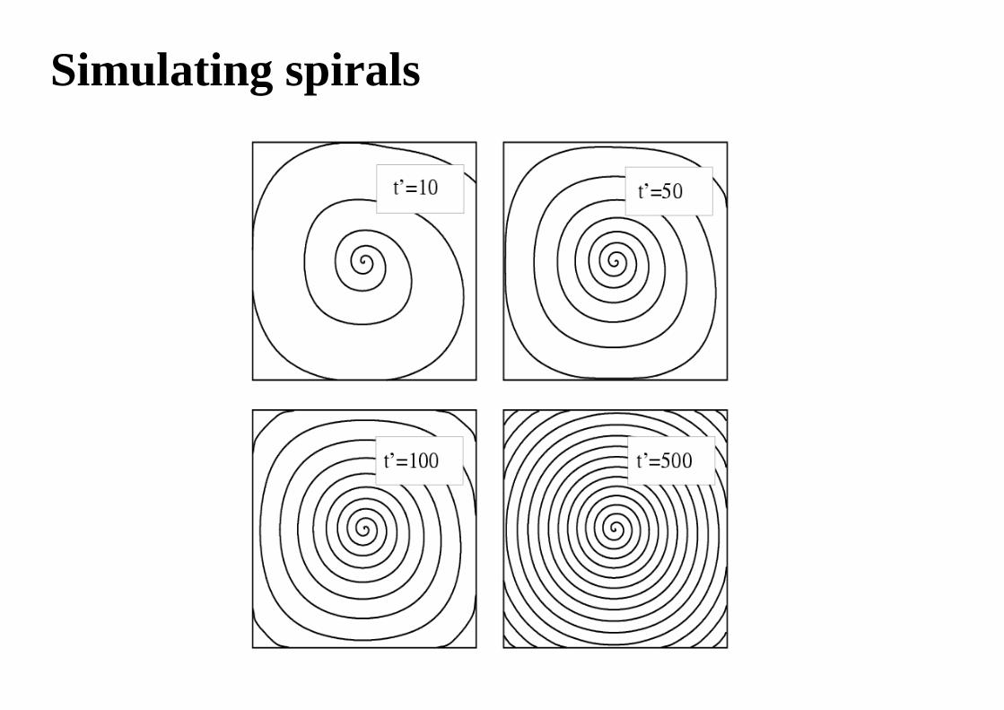
Simulating spirals

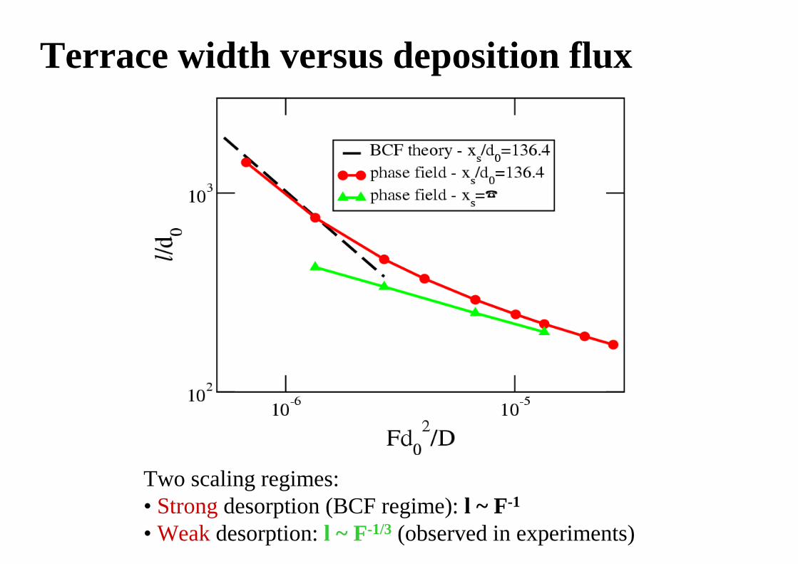
Terrace width versus deposition flux

Two scaling regimes:• Strongdesorption (BCF regime): l ~ F-1

• Weakdesorption: l ~ F-1/3 (observed in experiments)

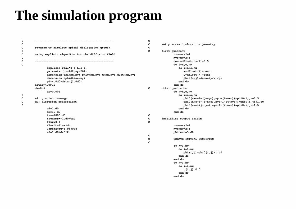
The simulation program

C ------------------------------------------- ----CC program to simulate spiral dislocation growthCC using explicit algorithm for the diffusion fieldCC ------------------------------------------- ----C

implicit real*8(a-h,o-z)parameter(nx=202,ny=202)dimension phi(nx,ny),phi0(nx,ny),u(nx,ny),dudt(nx,ny )dimension dphidt(nx,ny)pi=4.0d0*datan(1.0d0)

niter=400001dx=0.5

dt=0.005CC w2: gradient energyC du: diffusion coefficientC

w2=1.d0du=10.d0tau=1000.d0taudamp=-1.d0/tauflux=0.1fluxdt=flux*dtlambda=du*1.959088e2=1.d0/dx**2

CC setup screw dislocation geometryCC first quadrant

nxo=nx/2+1nyo=ny/2+1cent=dfloat(nx/2)+0.5do j=nyo,ny

do i=nxo,nxx=dfloat(i)-centy=dfloat(j)-centphi0(i,j)=datan(y/x)/pi

end doend do

C other quadrantsdo j=nyo,ny

do i=nxo,nxphi0(nxo-1-(j-nyo),nyo+(i-nxo))=phi0(i,j)+0.5phi0(nxo-1-(i-nxo),nyo-1-(j-nyo))=phi0(i,j)+1.d0phi0(nxo+(j-nyo),nyo-1-(i-nxo))=phi0(i,j)+1.5

end doend do

CC initialize output originC

nxo=nx/2+1nyo=ny/2+1phicent=3.d0

CC CREATE INITIAL CONDITIONC

do j=1,nydo i=1,nx

phi(i,j)=phi0(i,j)-1.d0end do

end dodo j=1,ny

do i=1,nxu(i,j)=0.0

end doend do

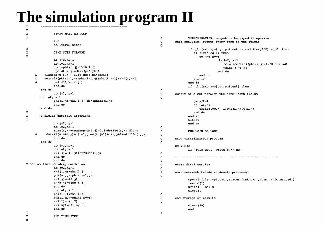
The simulation program IIC ------------------------------------------- ----CC START MAIN DO LOOPC

t=0do iter=0,niter

CC TIME STEP FORWARDC

do j=2,ny-1do i=2,nx-1dphi=phi(i,j)-phi0(i,j)dphidt(i,j)=dsin(pi*dphi)

& +lambda*u(i,j)*(1.d0+dcos(pi*dphi))& +e2*w2*(phi(i+1,j)+phi(i-1,j)+phi(i,j+1)+phi(i ,j-1)& -4.d0*phi(i,j))

end doend do

do j=2,ny-1do i=2,nx-1

phi(i,j)=phi(i,j)+dt*dphidt(i,j)end do

end doCC u field: explicit algorithm.C

do j=2,ny-1do i=2,nx-1dudt(i,j)=taudamp*u(i,j)-0.5*dphidt(i,j)+flux+

& du*e2*(u(i+1,j)+u(i-1,j)+u(i,j-1)+u(i,j+1)-4. d0*u(i,j))end do

end dodo j=2,ny-1do i=2,nx-1u(i,j)=u(i,j)+dt*dudt(i,j)end doend do

C BC: no flux boundary conditiondo j=2,ny-1phi(1,j)=phi(2,j)phi(nx,j)=phi(nx-1,j)u(1,j)=u(2,j)u(nx,j)=u(nx-1,j)end dodo i=2,nx-1phi(i,1)=phi(i,2)phi(i,ny)=phi(i,ny-1)u(i,1)=u(i,2)u(i,ny)=u(i,ny-1)end do

CC END TIME STEPC

C VISUALIZATION: output to be piped to spirvisC data analysis: output every turn of the spiralC

if (phi(nxo,nyo).gt.phicent.or.mod(iter,100).eq.0) t henif (ivis.eq.1) then

do j=2,ny-1do i=2,nx-1

nc = mod(int((phi(i,j)+1)*8.d0),64)write(6,*) nc

end doend do

end ifend ifif (phi(nxo,nyo).gt.phicent) then

CC output of a cut through the core: both fieldsC

j=ny/2+1do i=2,nx-1

write(100,*) i,phi(i,j),u(i,j)end do

end ift=t+dtend do

CC END MAIN DO LOOPCC stop visualization programC

nc = 230if (ivis.eq.1) write(6,*) nc

CC ------------------------------------------- -------------CC store final resultsCC save relevant fields in double precisionC

open(1,file='spi.out',status='unknown',form='unform atted')rewind(1)write(1) phi,uclose(1)

CC end storage of resultsC

close(20)end

C

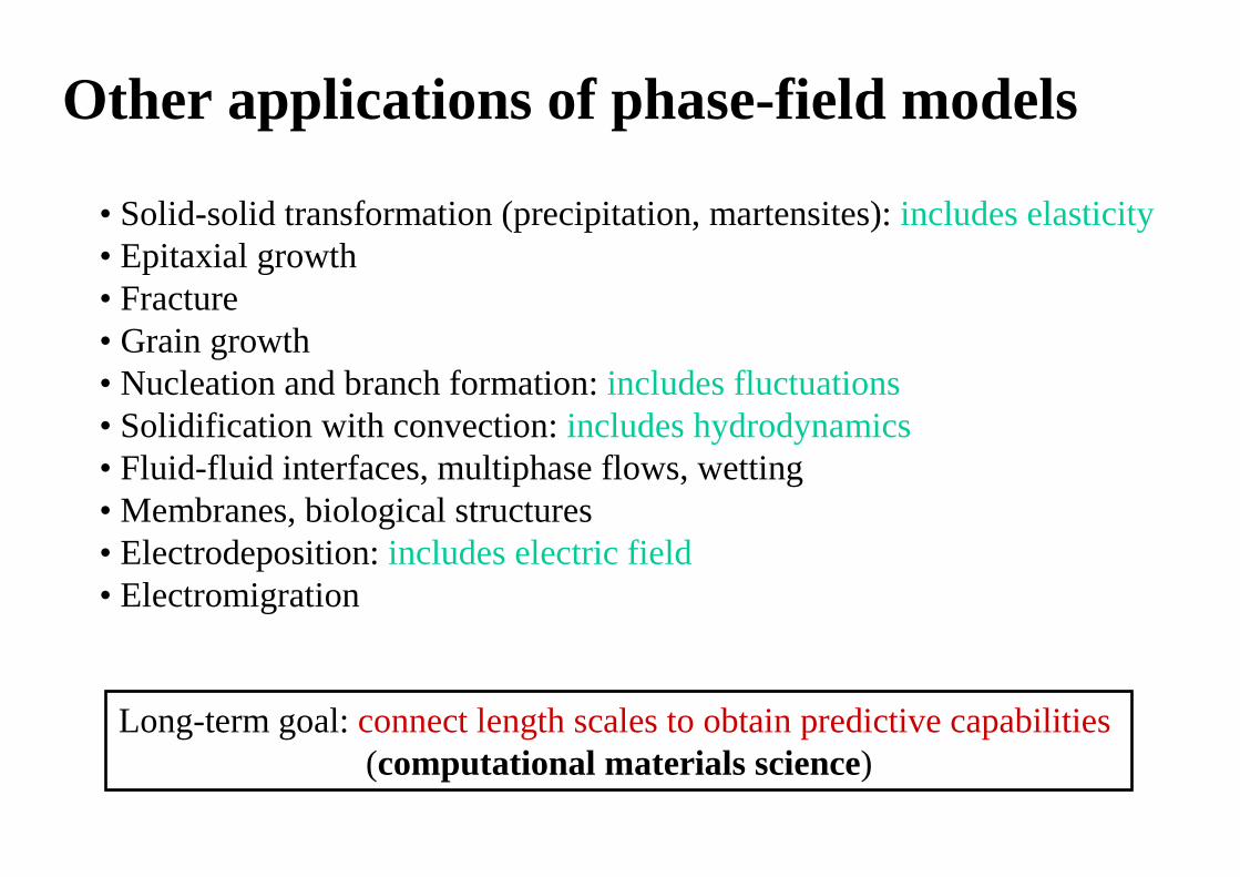
Other applications of phase-field models

• Solid-solid transformation (precipitation, martensites): includes elasticity• Epitaxial growth• Fracture• Grain growth• Nucleation and branch formation: includes fluctuations• Solidification with convection: includes hydrodynamics• Fluid-fluid interfaces, multiphase flows, wetting• Membranes, biological structures• Electrodeposition: includes electric field• Electromigration

Long-term goal: connect length scales to obtain predictive capabilities(computational materials science)

AcknowledgmentsCollaborators

• Marcus Dejmek, Roger Folch, Andrea Parisi, Jesper Mellenthin, Hervé Henry, Thi-Hanh Nguyen, Vincent Fleury(Laboratoire PMC, CNRS/Ecole Polytechnique)• Alain Karma, Jean Bragard, Youngyih Lee, Tak Shing Lo, Blas Echebarria (Physics Department, Northeastern University, Boston)• Gabriel Faivre, Silvère Akamatsu, Sabine Bottin-Rousseau(INSP, CNRS/Université Paris VI)

Support

Centre National de la Rescherche Scientifique (CNRS)Ecole PolytechniqueCentre National des Etudes Spatiales (CNES)