Geostatistics forLarge Data Sets

Whitney Huang

Motivation

MethodsCovariancetaperingLow–rankapproximationLikelihoodapproximationGaussian Markovrandom fieldapproximation

Geostatistical Modeling for Large Data Sets

Whitney Huang

Department of StatisticsPurdue University

October 28, 2014

Geostatistics forLarge Data Sets

Whitney Huang

Motivation

MethodsCovariancetaperingLow–rankapproximationLikelihoodapproximationGaussian Markovrandom fieldapproximation

Outline

Motivation

MethodsCovariance taperingLow–rank approximationLikelihood approximationGaussian Markov random field approximation

Geostatistics forLarge Data Sets

Whitney Huang

Motivation

MethodsCovariancetaperingLow–rankapproximationLikelihoodapproximationGaussian Markovrandom fieldapproximation

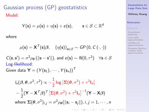
Gaussian process (GP) geostatisticsModel:

Y (s) = µ(s) + η(s) + ε(s), s ∈ S ⊂ Rd

where

µ(s) = XT (s)β, {η(s)}s∈S ∼ GP (0,C (·, ·))

C (s, s′) = σ2ρθ (‖s− s′‖), and ε(s) ∼ N(0, τ2) ∀s ∈ SLog-likelihood:Given data Y = (Y (s1), · · · ,Y (sn))T

ln(β,θ, σ2, τ2) ∝ −12log∣∣Σ(θ, σ2) + τ2In

∣∣− 1

2(Y− XTβ)T

[Σ(θ, σ2) + τ2In

]−1(Y− Xβ)

where Σ(θ, σ2)i ,j = σ2ρθ(‖si − sj‖), i , j = 1, · · · , n

Geostatistics forLarge Data Sets

Whitney Huang

Motivation

MethodsCovariancetaperingLow–rankapproximationLikelihoodapproximationGaussian Markovrandom fieldapproximation

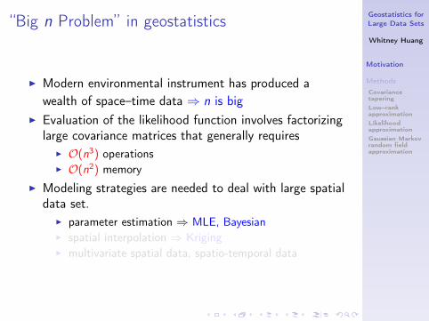
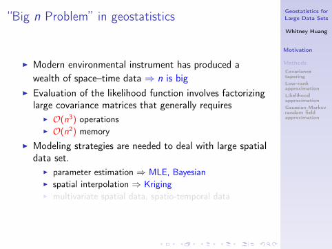
“Big n Problem” in geostatistics

I Modern environmental instrument has produced awealth of space–time data ⇒ n is big

I Evaluation of the likelihood function involves factorizinglarge covariance matrices that generally requires

I O(n3) operationsI O(n2) memory

I Modeling strategies are needed to deal with large spatialdata set.

I parameter estimation ⇒ MLE, BayesianI spatial interpolation ⇒ KrigingI multivariate spatial data, spatio-temporal data

Geostatistics forLarge Data Sets

Whitney Huang

Motivation

MethodsCovariancetaperingLow–rankapproximationLikelihoodapproximationGaussian Markovrandom fieldapproximation

“Big n Problem” in geostatistics

I Modern environmental instrument has produced awealth of space–time data ⇒ n is big

I Evaluation of the likelihood function involves factorizinglarge covariance matrices that generally requires

I O(n3) operationsI O(n2) memory

I Modeling strategies are needed to deal with large spatialdata set.

I parameter estimation ⇒ MLE, BayesianI spatial interpolation ⇒ KrigingI multivariate spatial data, spatio-temporal data

Geostatistics forLarge Data Sets

Whitney Huang

Motivation

MethodsCovariancetaperingLow–rankapproximationLikelihoodapproximationGaussian Markovrandom fieldapproximation

“Big n Problem” in geostatistics

I Modern environmental instrument has produced awealth of space–time data ⇒ n is big

I Evaluation of the likelihood function involves factorizinglarge covariance matrices that generally requires

I O(n3) operationsI O(n2) memory

I Modeling strategies are needed to deal with large spatialdata set.

I parameter estimation ⇒ MLE, BayesianI spatial interpolation ⇒ KrigingI multivariate spatial data, spatio-temporal data

Geostatistics forLarge Data Sets

Whitney Huang

Motivation

MethodsCovariancetaperingLow–rankapproximationLikelihoodapproximationGaussian Markovrandom fieldapproximation

Modeling strategies in the literature

I Covariance tapering (Furrer et al. 06, Kaufman et al.08, Du et al. 09)

I Low–rank approximation (Cressie & Johannesson 08,Banerjee et al. 08)

I Likelihood approximation (Vecchia 88, Stein 04)

I Gaussian Markov random field approximation (Rue &Tjelmeland 02, Rue & Held 05, Lindgren et al. 11)

Geostatistics forLarge Data Sets

Whitney Huang

Motivation

MethodsCovariancetaperingLow–rankapproximationLikelihoodapproximationGaussian Markovrandom fieldapproximation

Modeling strategies in the literature

I Covariance tapering (Furrer et al. 06, Kaufman et al.08, Du et al. 09)

I Low–rank approximation (Cressie & Johannesson 08,Banerjee et al. 08)

I Likelihood approximation (Vecchia 88, Stein 04)

I Gaussian Markov random field approximation (Rue &Tjelmeland 02, Rue & Held 05, Lindgren et al. 11)

Geostatistics forLarge Data Sets

Whitney Huang

Motivation

MethodsCovariancetaperingLow–rankapproximationLikelihoodapproximationGaussian Markovrandom fieldapproximation

Modeling strategies in the literature

I Covariance tapering (Furrer et al. 06, Kaufman et al.08, Du et al. 09)

I Low–rank approximation (Cressie & Johannesson 08,Banerjee et al. 08)

I Likelihood approximation (Vecchia 88, Stein 04)

I Gaussian Markov random field approximation (Rue &Tjelmeland 02, Rue & Held 05, Lindgren et al. 11)

Geostatistics forLarge Data Sets

Whitney Huang

Motivation

MethodsCovariancetaperingLow–rankapproximationLikelihoodapproximationGaussian Markovrandom fieldapproximation

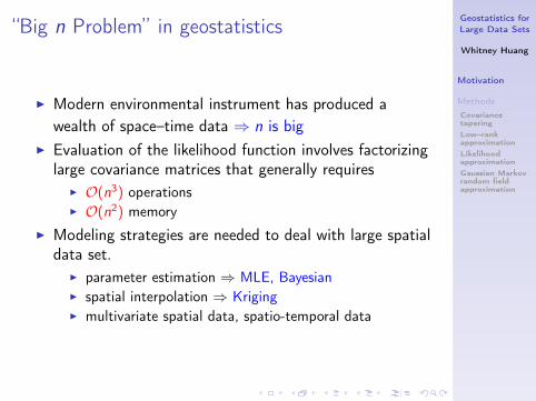
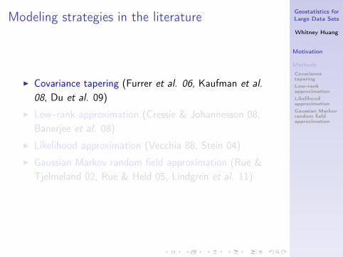
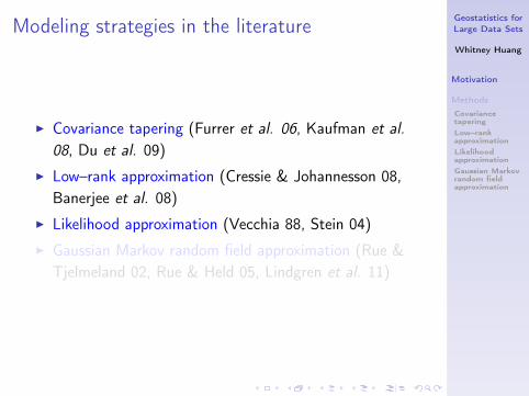
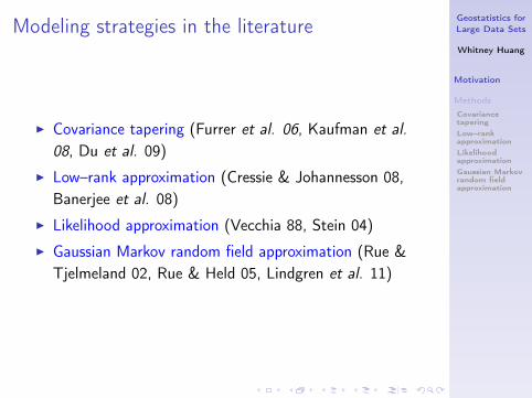
Modeling strategies in the literature

I Covariance tapering (Furrer et al. 06, Kaufman et al.08, Du et al. 09)

I Low–rank approximation (Cressie & Johannesson 08,Banerjee et al. 08)

I Likelihood approximation (Vecchia 88, Stein 04)

I Gaussian Markov random field approximation (Rue &Tjelmeland 02, Rue & Held 05, Lindgren et al. 11)

Geostatistics forLarge Data Sets

Whitney Huang

Motivation

MethodsCovariancetaperingLow–rankapproximationLikelihoodapproximationGaussian Markovrandom fieldapproximation

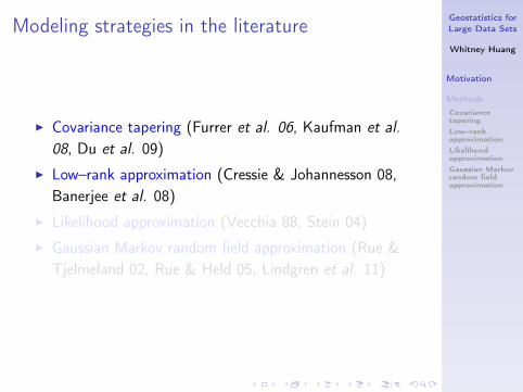
Outline

Motivation

MethodsCovariance taperingLow–rank approximationLikelihood approximationGaussian Markov random field approximation

Geostatistics forLarge Data Sets

Whitney Huang

Motivation

MethodsCovariancetaperingLow–rankapproximationLikelihoodapproximationGaussian Markovrandom fieldapproximation

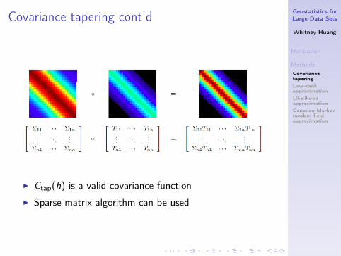
Covariance tapering (Furrer et al. 06)We replace the C (‖h‖) by

Ctap(h; γ) = ρtap(h; γ) ◦ C (h)

where ρtap(h; γ) is an isotropic correlation function withcompact support (ρtap(h) = 0 if h ≥ γ) and ◦ denotes theSchur product

Geostatistics forLarge Data Sets

Whitney Huang

Motivation

MethodsCovariancetaperingLow–rankapproximationLikelihoodapproximationGaussian Markovrandom fieldapproximation

Covariance tapering cont’d

I Ctap(h) is a valid covariance function

I Sparse matrix algorithm can be used

Geostatistics forLarge Data Sets

Whitney Huang

Motivation

MethodsCovariancetaperingLow–rankapproximationLikelihoodapproximationGaussian Markovrandom fieldapproximation

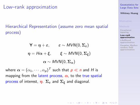
Low–rank approximation

Hierarchical Representation (assume zero mean spatialprocess)

Y = η + ε, ε ∼ MVN(0,Σε)

η = Hα+ ξ, ξ ∼ MVN(0,Σξ)

α ∼ MVN(0,Σα)

where α = (α1, · · · , αp)T such that p � n and H ismapping from the latent process, α, to the true spatialprocess of interest, η. Σε and Σξ and diagonal.

Geostatistics forLarge Data Sets

Whitney Huang

Motivation

MethodsCovariancetaperingLow–rankapproximationLikelihoodapproximationGaussian Markovrandom fieldapproximation

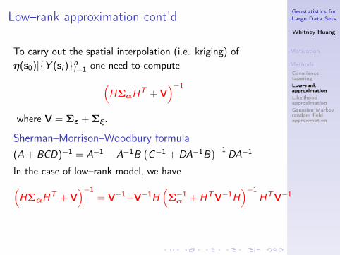
Low–rank approximation cont’d

To carry out the spatial interpolation (i.e. kriging) ofη(s0)|{Y (si )}ni=1 one need to compute(

HΣαHT + V

)−1

where V = Σε + Σξ.

Sherman–Morrison–Woodbury formula(A + BCD)−1 = A−1 − A−1B

(C−1 + DA−1B

)−1DA−1

In the case of low–rank model, we have(HΣαH

T + V)−1

= V−1−V−1H(Σ−1α + HTV−1H

)−1HTV−1

Geostatistics forLarge Data Sets

Whitney Huang

Motivation

MethodsCovariancetaperingLow–rankapproximationLikelihoodapproximationGaussian Markovrandom fieldapproximation

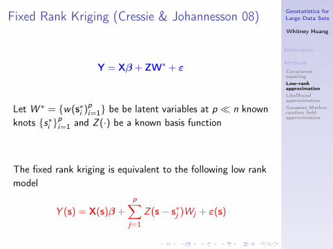
Fixed Rank Kriging (Cressie & Johannesson 08)

Y = Xβ + ZW∗ + ε

Let W ∗ = {w(s∗i )pi=1} be be latent variables at p � n knownknots {s∗i }

pi=1 and Z (·) be a known basis function

The fixed rank kriging is equivalent to the following low rankmodel

Y (s) = X(s)β +

p∑j=1

Z (s− s∗j )Wj + ε(s)

Geostatistics forLarge Data Sets

Whitney Huang

Motivation

MethodsCovariancetaperingLow–rankapproximationLikelihoodapproximationGaussian Markovrandom fieldapproximation

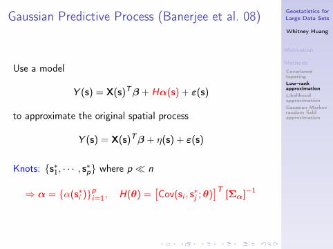
Gaussian Predictive Process (Banerjee et al. 08)

Use a model

Y (s) = X(s)Tβ + Hα(s) + ε(s)

to approximate the original spatial process

Y (s) = X(s)Tβ + η(s) + ε(s)

Knots: {s∗1, · · · , s∗p} where p � n

⇒ α = {α(s∗i )}pi=1, H(θ) =[Cov(si , s∗j ;θ)

]T[Σα]−1

Geostatistics forLarge Data Sets

Whitney Huang

Motivation

MethodsCovariancetaperingLow–rankapproximationLikelihoodapproximationGaussian Markovrandom fieldapproximation

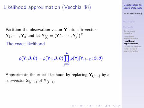
Likelihood approximation (Vecchia 88)

Partition the observation vector Y into sub–vectorY1, · · · ,Yb and let Y(j) = (YT

1 , · · · ,YTj )T

The exact likelihood

p(Y;β,θ) = p(Y1;β,θ)b∏

j=2

p(Yj |Y(j−1);β,θ)

Approximate the exact likelihood by replacing Y(j−1) by asub–vector S(j−1) of Y(j−1)

Geostatistics forLarge Data Sets

Whitney Huang

Motivation

MethodsCovariancetaperingLow–rankapproximationLikelihoodapproximationGaussian Markovrandom fieldapproximation

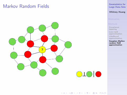
Markov Random Fields

Geostatistics forLarge Data Sets

Whitney Huang

Motivation

MethodsCovariancetaperingLow–rankapproximationLikelihoodapproximationGaussian Markovrandom fieldapproximation

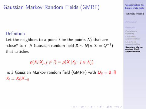
Gaussian Markov Random Fields (GMRF)

DefinitionLet the neighbors to a point i be the points Ni that are“close" to i . A Gaussian random field X ∼ N(µ,Σ = Q−1)

that satisfies

p(Xi |Xj , j 6= i) = p(Xi |Xj : j ∈ Nj)

is a Gaussian Markov random field (GMRF) with Qij = 0 iffXi ⊥ Xj |X−ij

Geostatistics forLarge Data Sets

Whitney Huang

Motivation

MethodsCovariancetaperingLow–rankapproximationLikelihoodapproximationGaussian Markovrandom fieldapproximation

Remarks: GP vs. GMRF in geostatistical modeling

I +: GP model is widely used in modeling continuouslyindexed spatial data in which the covariance functioncharacterizes the process properties

I –: Inference involves factorizing covariance matrices

I +: GMRF model is computationally efficient due to thesparse precision matrix

I –: Only for discretely indexed spatial data

Main idea of GMRF approach:

GP︸︷︷︸inference

SPDE⇐⇒ GMRF︸ ︷︷ ︸computation

Geostatistics forLarge Data Sets

Whitney Huang

Motivation

MethodsCovariancetaperingLow–rankapproximationLikelihoodapproximationGaussian Markovrandom fieldapproximation

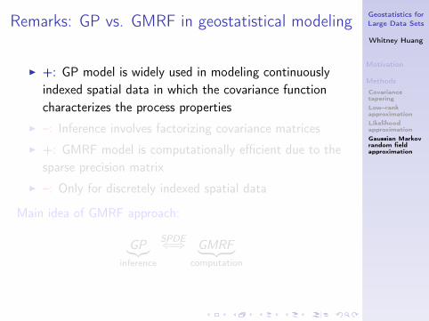
Remarks: GP vs. GMRF in geostatistical modeling

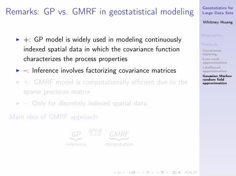
I +: GP model is widely used in modeling continuouslyindexed spatial data in which the covariance functioncharacterizes the process properties

I –: Inference involves factorizing covariance matrices

I +: GMRF model is computationally efficient due to thesparse precision matrix

I –: Only for discretely indexed spatial data

Main idea of GMRF approach:

GP︸︷︷︸inference

SPDE⇐⇒ GMRF︸ ︷︷ ︸computation

Geostatistics forLarge Data Sets

Whitney Huang

Motivation

MethodsCovariancetaperingLow–rankapproximationLikelihoodapproximationGaussian Markovrandom fieldapproximation

Remarks: GP vs. GMRF in geostatistical modeling

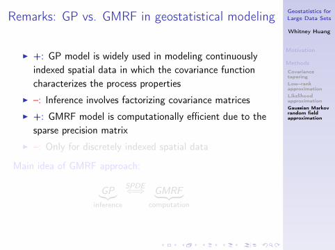
I +: GP model is widely used in modeling continuouslyindexed spatial data in which the covariance functioncharacterizes the process properties

I –: Inference involves factorizing covariance matrices

I +: GMRF model is computationally efficient due to thesparse precision matrix

I –: Only for discretely indexed spatial data

Main idea of GMRF approach:

GP︸︷︷︸inference

SPDE⇐⇒ GMRF︸ ︷︷ ︸computation

Geostatistics forLarge Data Sets

Whitney Huang

Motivation

MethodsCovariancetaperingLow–rankapproximationLikelihoodapproximationGaussian Markovrandom fieldapproximation

Remarks: GP vs. GMRF in geostatistical modeling

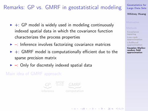
I +: GP model is widely used in modeling continuouslyindexed spatial data in which the covariance functioncharacterizes the process properties

I –: Inference involves factorizing covariance matrices

I +: GMRF model is computationally efficient due to thesparse precision matrix

I –: Only for discretely indexed spatial data

Main idea of GMRF approach:

GP︸︷︷︸inference

SPDE⇐⇒ GMRF︸ ︷︷ ︸computation

Geostatistics forLarge Data Sets

Whitney Huang

Motivation

MethodsCovariancetaperingLow–rankapproximationLikelihoodapproximationGaussian Markovrandom fieldapproximation

Remarks: GP vs. GMRF in geostatistical modeling

I +: GP model is widely used in modeling continuouslyindexed spatial data in which the covariance functioncharacterizes the process properties

I –: Inference involves factorizing covariance matrices

I +: GMRF model is computationally efficient due to thesparse precision matrix

I –: Only for discretely indexed spatial data

Main idea of GMRF approach:

GP︸︷︷︸inference

SPDE⇐⇒ GMRF︸ ︷︷ ︸computation

Geostatistics forLarge Data Sets

Whitney Huang

Motivation

MethodsCovariancetaperingLow–rankapproximationLikelihoodapproximationGaussian Markovrandom fieldapproximation

Remarks: GP vs. GMRF in geostatistical modeling

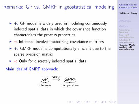
I +: GP model is widely used in modeling continuouslyindexed spatial data in which the covariance functioncharacterizes the process properties

I –: Inference involves factorizing covariance matrices

I +: GMRF model is computationally efficient due to thesparse precision matrix

I –: Only for discretely indexed spatial data

Main idea of GMRF approach:

GP︸︷︷︸inference

SPDE⇐⇒ GMRF︸ ︷︷ ︸computation

Geostatistics forLarge Data Sets

Whitney Huang

Motivation

MethodsCovariancetaperingLow–rankapproximationLikelihoodapproximationGaussian Markovrandom fieldapproximation

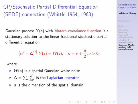
GP/Stochastic Partial Differential Equation(SPDE) connection (Whittle 1954, 1963)

Gaussian process Y (s) with Matern covariance function is astationary solution to the linear fractional stochastic partialdifferential equation:(

α2 −∆)κ

2 Y (s) =W(s), κ = ν +d

2, ν > 0

where

I W(s) is a spatial Gaussian white noise

I ∆ =∑

i∂2

∂s2iis the Laplacian operator

I d is the dimension of the spatial domain

Geostatistics forLarge Data Sets

Whitney Huang

Motivation

MethodsCovariancetaperingLow–rankapproximationLikelihoodapproximationGaussian Markovrandom fieldapproximation

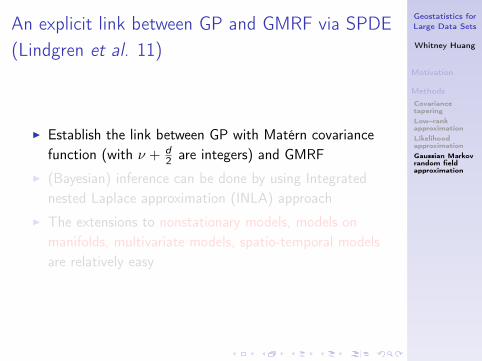
An explicit link between GP and GMRF via SPDE(Lindgren et al. 11)

I Establish the link between GP with Matérn covariancefunction (with ν + d

2 are integers) and GMRF

I (Bayesian) inference can be done by using Integratednested Laplace approximation (INLA) approach

I The extensions to nonstationary models, models onmanifolds, multivariate models, spatio-temporal modelsare relatively easy

Geostatistics forLarge Data Sets

Whitney Huang

Motivation

MethodsCovariancetaperingLow–rankapproximationLikelihoodapproximationGaussian Markovrandom fieldapproximation

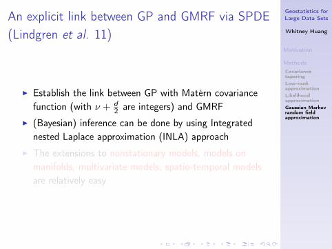
An explicit link between GP and GMRF via SPDE(Lindgren et al. 11)

I Establish the link between GP with Matérn covariancefunction (with ν + d

2 are integers) and GMRF

I (Bayesian) inference can be done by using Integratednested Laplace approximation (INLA) approach

I The extensions to nonstationary models, models onmanifolds, multivariate models, spatio-temporal modelsare relatively easy

Geostatistics forLarge Data Sets

Whitney Huang

Motivation

MethodsCovariancetaperingLow–rankapproximationLikelihoodapproximationGaussian Markovrandom fieldapproximation

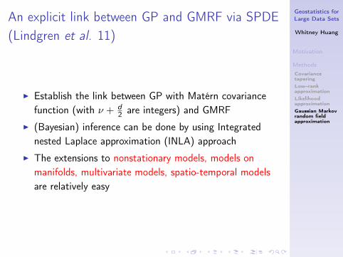
An explicit link between GP and GMRF via SPDE(Lindgren et al. 11)

I Establish the link between GP with Matérn covariancefunction (with ν + d

2 are integers) and GMRF

I (Bayesian) inference can be done by using Integratednested Laplace approximation (INLA) approach

I The extensions to nonstationary models, models onmanifolds, multivariate models, spatio-temporal modelsare relatively easy

Geostatistics forLarge Data Sets

Whitney Huang

Motivation

MethodsCovariancetaperingLow–rankapproximationLikelihoodapproximationGaussian Markovrandom fieldapproximation

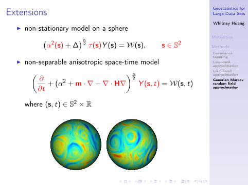
ExtensionsI non-stationary model on a sphere(

α2(s) + ∆)κ

2 τ(s)Y (s) =W(s), s ∈ S2

I non-separable anisotropic space-time model(∂

∂t+ (α2 + m · ∇ −∇ ·H∇

)κ2

Y (s, t) =W(s, t)

where (s, t) ∈ S2 × R

Geostatistics forLarge Data Sets

Whitney Huang

AppendixFor FurtherReading

For Further Reading I

H. Rue, and L. HeldGaussian Markov Random Fields: Theory andApplications.Chapman & Hall/CRC, 2005.

S. Banerjee, A. E. Gelfand, A. O. Finley, and H. SangGaussian Predictive Process Models for Large SpatialData SetsJRSSB, 70:825–848, 2008.

N. A. C. Cressie, and G. JohannessonFixed Rank Kriging for Very Large Spatial Data SetsJRSSB, 70:209–226, 2008.

Geostatistics forLarge Data Sets

Whitney Huang

AppendixFor FurtherReading

For Further Reading II

J. Du, H. Zhang, and V. S. MandrekarFixed–Domain Asymptotic Properties of TaperedMaximum Likelihood EstimatorsThe Annals of Statistics, 37:3330–3361, 2009.

R. Furrer, M. G. Genton, and D. W. NychkaCovariance Tapering for Interpolation of Large SpatialDatasetsJournal of Computational and Graphical Statistics,15:502–523, 2006.

C. G. Kaufman, M. J. Schervish, and D. W. NychkaCovariance Tapering for Likelihood–Based Estimation inLarge Spatial Data SetsJournal of the American Statistical Association,103:1545–1555, 2008.

Geostatistics forLarge Data Sets

Whitney Huang

AppendixFor FurtherReading

For Further Reading III

Lindgren, F., Rue, H., & Lindström, J.An explicit link between Gaussian fields and GaussianMarkov random fields: the stochastic partial differentialequation approach.JRSSB, 73:423–498

H. Rue, and H. TjelmelandFitting Gaussian Markov Random Fields to GaussianField.Scandinavian Journal of Statistics, 29:31–49

M. L. Stein, Z. Chi, and L. J. WeltyApproximating Likelihoods for Large Spatial Data SetsJRSSB, 66:275–296, 2004.

Geostatistics forLarge Data Sets

Whitney Huang

AppendixFor FurtherReading

For Further Reading IV

A. V. VecchiaEstimation and Model Identification for ContinuousSpatial ProcessesJRSSB, 50:297–312, 1988.