Geostatistics for Large Data Sets ...
35
Geostatistics for Large Data Sets Whitney Huang Motivation Methods Covariance tapering Low–rank approximation Likelihood approximation Gaussian Markov random field approximation Geostatistical Modeling for Large Data Sets Whitney Huang Department of Statistics Purdue University October 28, 2014
Transcript of Geostatistics for Large Data Sets ...
Geostatistics forLarge Data Sets
Whitney Huang
Motivation
MethodsCovariancetaperingLow–rankapproximationLikelihoodapproximationGaussian Markovrandom fieldapproximation
Geostatistical Modeling for Large Data Sets
Whitney Huang
Department of StatisticsPurdue University
October 28, 2014
Geostatistics forLarge Data Sets
Whitney Huang
Motivation
MethodsCovariancetaperingLow–rankapproximationLikelihoodapproximationGaussian Markovrandom fieldapproximation
Outline
Motivation
MethodsCovariance taperingLow–rank approximationLikelihood approximationGaussian Markov random field approximation
Geostatistics forLarge Data Sets
Whitney Huang
Motivation
MethodsCovariancetaperingLow–rankapproximationLikelihoodapproximationGaussian Markovrandom fieldapproximation
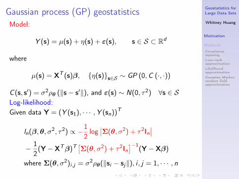
Gaussian process (GP) geostatisticsModel:
Y (s) = µ(s) + η(s) + ε(s), s ∈ S ⊂ Rd
where
µ(s) = XT (s)β, {η(s)}s∈S ∼ GP (0,C (·, ·))
C (s, s′) = σ2ρθ (‖s− s′‖), and ε(s) ∼ N(0, τ2) ∀s ∈ SLog-likelihood:Given data Y = (Y (s1), · · · ,Y (sn))T
ln(β,θ, σ2, τ2) ∝ −12log∣∣Σ(θ, σ2) + τ2In
∣∣− 1
2(Y− XTβ)T
[Σ(θ, σ2) + τ2In
]−1(Y− Xβ)
where Σ(θ, σ2)i ,j = σ2ρθ(‖si − sj‖), i , j = 1, · · · , n
Geostatistics forLarge Data Sets
Whitney Huang
Motivation
MethodsCovariancetaperingLow–rankapproximationLikelihoodapproximationGaussian Markovrandom fieldapproximation
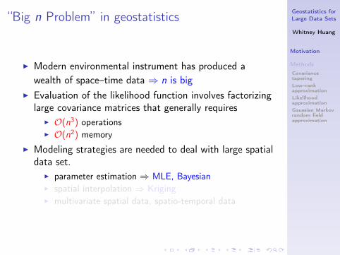
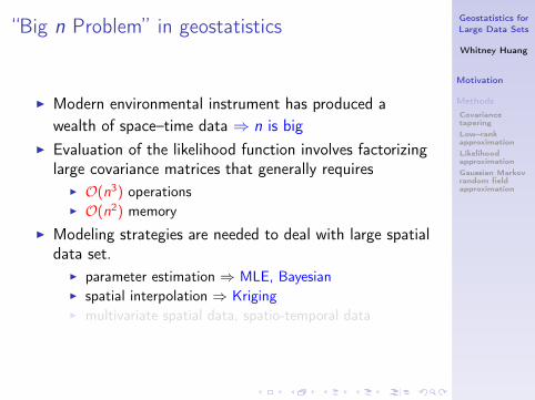
“Big n Problem” in geostatistics
I Modern environmental instrument has produced awealth of space–time data ⇒ n is big
I Evaluation of the likelihood function involves factorizinglarge covariance matrices that generally requires
I O(n3) operationsI O(n2) memory
I Modeling strategies are needed to deal with large spatialdata set.
I parameter estimation ⇒ MLE, BayesianI spatial interpolation ⇒ KrigingI multivariate spatial data, spatio-temporal data
Geostatistics forLarge Data Sets
Whitney Huang
Motivation
MethodsCovariancetaperingLow–rankapproximationLikelihoodapproximationGaussian Markovrandom fieldapproximation
Modeling strategies in the literature
I Covariance tapering (Furrer et al. 06, Kaufman et al.08, Du et al. 09)
I Low–rank approximation (Cressie & Johannesson 08,Banerjee et al. 08)
I Likelihood approximation (Vecchia 88, Stein 04)
I Gaussian Markov random field approximation (Rue &Tjelmeland 02, Rue & Held 05, Lindgren et al. 11)
Geostatistics forLarge Data Sets
Whitney Huang
Motivation
MethodsCovariancetaperingLow–rankapproximationLikelihoodapproximationGaussian Markovrandom fieldapproximation
Outline
Motivation
MethodsCovariance taperingLow–rank approximationLikelihood approximationGaussian Markov random field approximation

Geostatistics forLarge Data Sets
Whitney Huang
Motivation
MethodsCovariancetaperingLow–rankapproximationLikelihoodapproximationGaussian Markovrandom fieldapproximation
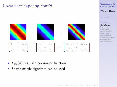
Covariance tapering (Furrer et al. 06)We replace the C (‖h‖) by
Ctap(h; γ) = ρtap(h; γ) ◦ C (h)
where ρtap(h; γ) is an isotropic correlation function withcompact support (ρtap(h) = 0 if h ≥ γ) and ◦ denotes theSchur product
Geostatistics forLarge Data Sets
Whitney Huang
Motivation
MethodsCovariancetaperingLow–rankapproximationLikelihoodapproximationGaussian Markovrandom fieldapproximation
Covariance tapering cont’d
I Ctap(h) is a valid covariance function
I Sparse matrix algorithm can be used
Geostatistics forLarge Data Sets
Whitney Huang
Motivation
MethodsCovariancetaperingLow–rankapproximationLikelihoodapproximationGaussian Markovrandom fieldapproximation
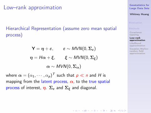
Low–rank approximation
Hierarchical Representation (assume zero mean spatialprocess)
Y = η + ε, ε ∼ MVN(0,Σε)
η = Hα+ ξ, ξ ∼ MVN(0,Σξ)
α ∼ MVN(0,Σα)
where α = (α1, · · · , αp)T such that p � n and H ismapping from the latent process, α, to the true spatialprocess of interest, η. Σε and Σξ and diagonal.
Geostatistics forLarge Data Sets
Whitney Huang
Motivation
MethodsCovariancetaperingLow–rankapproximationLikelihoodapproximationGaussian Markovrandom fieldapproximation
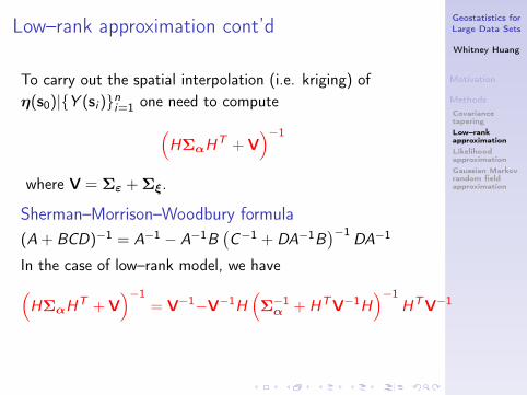
Low–rank approximation cont’d
To carry out the spatial interpolation (i.e. kriging) ofη(s0)|{Y (si )}ni=1 one need to compute(
HΣαHT + V
)−1
where V = Σε + Σξ.
Sherman–Morrison–Woodbury formula(A + BCD)−1 = A−1 − A−1B
(C−1 + DA−1B
)−1DA−1
In the case of low–rank model, we have(HΣαH
T + V)−1
= V−1−V−1H(Σ−1α + HTV−1H
)−1HTV−1
Geostatistics forLarge Data Sets
Whitney Huang
Motivation
MethodsCovariancetaperingLow–rankapproximationLikelihoodapproximationGaussian Markovrandom fieldapproximation
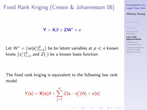
Fixed Rank Kriging (Cressie & Johannesson 08)
Y = Xβ + ZW∗ + ε
Let W ∗ = {w(s∗i )pi=1} be be latent variables at p � n knownknots {s∗i }
pi=1 and Z (·) be a known basis function
The fixed rank kriging is equivalent to the following low rankmodel
Y (s) = X(s)β +
p∑j=1
Z (s− s∗j )Wj + ε(s)
Geostatistics forLarge Data Sets
Whitney Huang
Motivation
MethodsCovariancetaperingLow–rankapproximationLikelihoodapproximationGaussian Markovrandom fieldapproximation
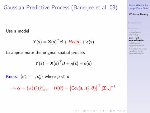
Gaussian Predictive Process (Banerjee et al. 08)
Use a model
Y (s) = X(s)Tβ + Hα(s) + ε(s)
to approximate the original spatial process
Y (s) = X(s)Tβ + η(s) + ε(s)
Knots: {s∗1, · · · , s∗p} where p � n
⇒ α = {α(s∗i )}pi=1, H(θ) =[Cov(si , s∗j ;θ)
]T[Σα]−1
Geostatistics forLarge Data Sets
Whitney Huang
Motivation
MethodsCovariancetaperingLow–rankapproximationLikelihoodapproximationGaussian Markovrandom fieldapproximation
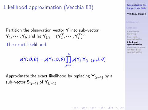
Likelihood approximation (Vecchia 88)
Partition the observation vector Y into sub–vectorY1, · · · ,Yb and let Y(j) = (YT
1 , · · · ,YTj )T
The exact likelihood
p(Y;β,θ) = p(Y1;β,θ)b∏
j=2
p(Yj |Y(j−1);β,θ)
Approximate the exact likelihood by replacing Y(j−1) by asub–vector S(j−1) of Y(j−1)
Geostatistics forLarge Data Sets
Whitney Huang
Motivation
MethodsCovariancetaperingLow–rankapproximationLikelihoodapproximationGaussian Markovrandom fieldapproximation
Markov Random Fields
Geostatistics forLarge Data Sets
Whitney Huang
Motivation
MethodsCovariancetaperingLow–rankapproximationLikelihoodapproximationGaussian Markovrandom fieldapproximation
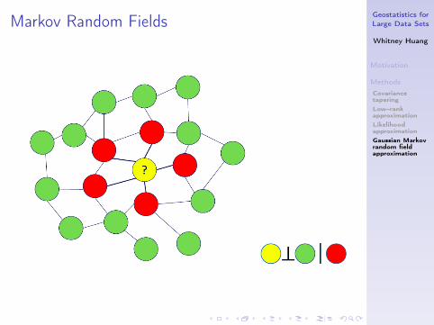
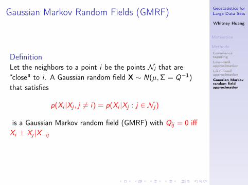
Gaussian Markov Random Fields (GMRF)
DefinitionLet the neighbors to a point i be the points Ni that are“close" to i . A Gaussian random field X ∼ N(µ,Σ = Q−1)
that satisfies
p(Xi |Xj , j 6= i) = p(Xi |Xj : j ∈ Nj)
is a Gaussian Markov random field (GMRF) with Qij = 0 iffXi ⊥ Xj |X−ij
Geostatistics forLarge Data Sets
Whitney Huang
Motivation
MethodsCovariancetaperingLow–rankapproximationLikelihoodapproximationGaussian Markovrandom fieldapproximation
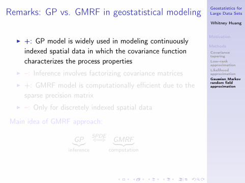
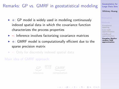
Remarks: GP vs. GMRF in geostatistical modeling
I +: GP model is widely used in modeling continuouslyindexed spatial data in which the covariance functioncharacterizes the process properties
I –: Inference involves factorizing covariance matrices
I +: GMRF model is computationally efficient due to thesparse precision matrix
I –: Only for discretely indexed spatial data
Main idea of GMRF approach:
GP︸︷︷︸inference
SPDE⇐⇒ GMRF︸ ︷︷ ︸computation
Geostatistics forLarge Data Sets
Whitney Huang
Motivation
MethodsCovariancetaperingLow–rankapproximationLikelihoodapproximationGaussian Markovrandom fieldapproximation
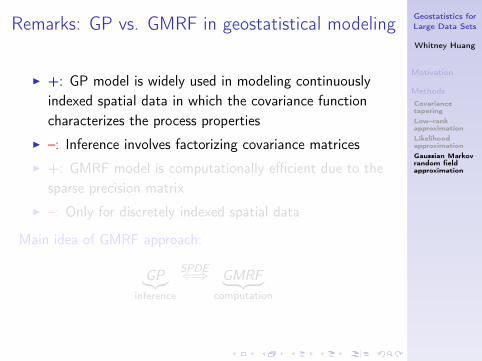
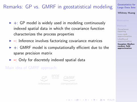
Remarks: GP vs. GMRF in geostatistical modeling
I +: GP model is widely used in modeling continuouslyindexed spatial data in which the covariance functioncharacterizes the process properties
I –: Inference involves factorizing covariance matrices
I +: GMRF model is computationally efficient due to thesparse precision matrix
I –: Only for discretely indexed spatial data
Main idea of GMRF approach:
GP︸︷︷︸inference
SPDE⇐⇒ GMRF︸ ︷︷ ︸computation
Geostatistics forLarge Data Sets
Whitney Huang
Motivation
MethodsCovariancetaperingLow–rankapproximationLikelihoodapproximationGaussian Markovrandom fieldapproximation
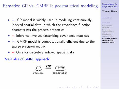
Remarks: GP vs. GMRF in geostatistical modeling
I +: GP model is widely used in modeling continuouslyindexed spatial data in which the covariance functioncharacterizes the process properties
I –: Inference involves factorizing covariance matrices
I +: GMRF model is computationally efficient due to thesparse precision matrix
I –: Only for discretely indexed spatial data
Main idea of GMRF approach:
GP︸︷︷︸inference
SPDE⇐⇒ GMRF︸ ︷︷ ︸computation

Geostatistics forLarge Data Sets
Whitney Huang
Motivation
MethodsCovariancetaperingLow–rankapproximationLikelihoodapproximationGaussian Markovrandom fieldapproximation
Remarks: GP vs. GMRF in geostatistical modeling
I +: GP model is widely used in modeling continuouslyindexed spatial data in which the covariance functioncharacterizes the process properties
I –: Inference involves factorizing covariance matrices
I +: GMRF model is computationally efficient due to thesparse precision matrix
I –: Only for discretely indexed spatial data
Main idea of GMRF approach:
GP︸︷︷︸inference
SPDE⇐⇒ GMRF︸ ︷︷ ︸computation
Geostatistics forLarge Data Sets
Whitney Huang
Motivation
MethodsCovariancetaperingLow–rankapproximationLikelihoodapproximationGaussian Markovrandom fieldapproximation
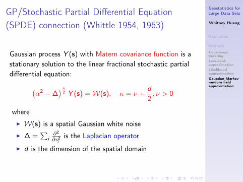
GP/Stochastic Partial Differential Equation(SPDE) connection (Whittle 1954, 1963)
Gaussian process Y (s) with Matern covariance function is astationary solution to the linear fractional stochastic partialdifferential equation:(
α2 −∆)κ
2 Y (s) =W(s), κ = ν +d
2, ν > 0
where
I W(s) is a spatial Gaussian white noise
I ∆ =∑
i∂2
∂s2iis the Laplacian operator
I d is the dimension of the spatial domain
Geostatistics forLarge Data Sets
Whitney Huang
Motivation
MethodsCovariancetaperingLow–rankapproximationLikelihoodapproximationGaussian Markovrandom fieldapproximation
An explicit link between GP and GMRF via SPDE(Lindgren et al. 11)
I Establish the link between GP with Matérn covariancefunction (with ν + d
2 are integers) and GMRF
I (Bayesian) inference can be done by using Integratednested Laplace approximation (INLA) approach
I The extensions to nonstationary models, models onmanifolds, multivariate models, spatio-temporal modelsare relatively easy
Geostatistics forLarge Data Sets
Whitney Huang
Motivation
MethodsCovariancetaperingLow–rankapproximationLikelihoodapproximationGaussian Markovrandom fieldapproximation
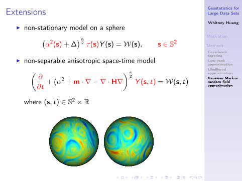
ExtensionsI non-stationary model on a sphere(
α2(s) + ∆)κ
2 τ(s)Y (s) =W(s), s ∈ S2
I non-separable anisotropic space-time model(∂
∂t+ (α2 + m · ∇ −∇ ·H∇
)κ2
Y (s, t) =W(s, t)
where (s, t) ∈ S2 × R
Geostatistics forLarge Data Sets
Whitney Huang
AppendixFor FurtherReading
For Further Reading I
H. Rue, and L. HeldGaussian Markov Random Fields: Theory andApplications.Chapman & Hall/CRC, 2005.
S. Banerjee, A. E. Gelfand, A. O. Finley, and H. SangGaussian Predictive Process Models for Large SpatialData SetsJRSSB, 70:825–848, 2008.
N. A. C. Cressie, and G. JohannessonFixed Rank Kriging for Very Large Spatial Data SetsJRSSB, 70:209–226, 2008.
Geostatistics forLarge Data Sets
Whitney Huang
AppendixFor FurtherReading
For Further Reading II
J. Du, H. Zhang, and V. S. MandrekarFixed–Domain Asymptotic Properties of TaperedMaximum Likelihood EstimatorsThe Annals of Statistics, 37:3330–3361, 2009.
R. Furrer, M. G. Genton, and D. W. NychkaCovariance Tapering for Interpolation of Large SpatialDatasetsJournal of Computational and Graphical Statistics,15:502–523, 2006.
C. G. Kaufman, M. J. Schervish, and D. W. NychkaCovariance Tapering for Likelihood–Based Estimation inLarge Spatial Data SetsJournal of the American Statistical Association,103:1545–1555, 2008.
Geostatistics forLarge Data Sets
Whitney Huang
AppendixFor FurtherReading
For Further Reading III
Lindgren, F., Rue, H., & Lindström, J.An explicit link between Gaussian fields and GaussianMarkov random fields: the stochastic partial differentialequation approach.JRSSB, 73:423–498
H. Rue, and H. TjelmelandFitting Gaussian Markov Random Fields to GaussianField.Scandinavian Journal of Statistics, 29:31–49
M. L. Stein, Z. Chi, and L. J. WeltyApproximating Likelihoods for Large Spatial Data SetsJRSSB, 66:275–296, 2004.
Geostatistics forLarge Data Sets
Whitney Huang
AppendixFor FurtherReading
For Further Reading IV
A. V. VecchiaEstimation and Model Identification for ContinuousSpatial ProcessesJRSSB, 50:297–312, 1988.