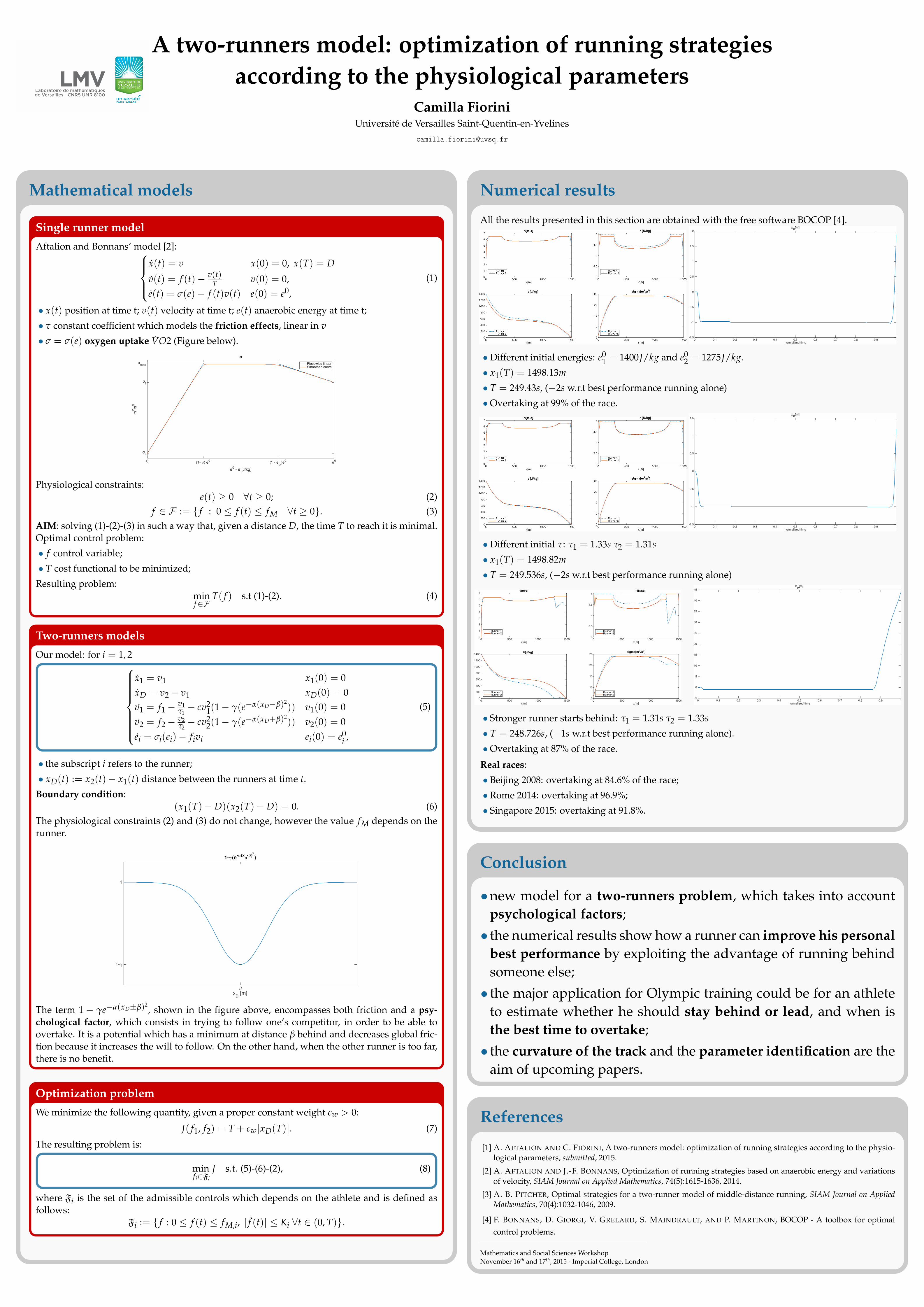
A two-runners model: optimization of running strategiesaccording to the physiological parameters

Camilla FioriniUniversité de Versailles Saint-Quentin-en-Yvelines

camilla.fiorini@uvsq.fr

Aftalion and Bonnans’ model [2]:x(t) = v x(0) = 0, x(T) = D

v(t) = f (t)− v(t)τ v(0) = 0,

e(t) = σ(e)− f (t)v(t) e(0) = e0,

(1)

• x(t) position at time t; v(t) velocity at time t; e(t) anaerobic energy at time t;

• τ constant coefficient which models the friction effects, linear in v

• σ = σ(e) oxygen uptake VO2 (Figure below).

e0 - e [J/kg]

0 (1- φ) e0

(1 - ecr

)e0

e0

m2/s

3

r

f

max Piecewise linearSmoothed curve

Physiological constraints:e(t) ≥ 0 ∀t ≥ 0; (2)

f ∈ F := { f : 0 ≤ f (t) ≤ fM ∀t ≥ 0}. (3)AIM: solving (1)-(2)-(3) in such a way that, given a distance D, the time T to reach it is minimal.Optimal control problem:

• f control variable;

• T cost functional to be minimized;

Resulting problem:minf∈F

T( f ) s.t (1)-(2). (4)

Single runner model

Our model: for i = 1, 2

x1 = v1 x1(0) = 0xD = v2− v1 xD(0) = 0v1 = f1− v1

τ1− cv2

1(1− γ(e−α(xD−β)2)) v1(0) = 0

v2 = f2− v2τ2− cv2

2(1− γ(e−α(xD+β)2)) v2(0) = 0

ei = σi(ei)− fivi ei(0) = e0i ,

(5)

• the subscript i refers to the runner;

• xD(t) := x2(t)− x1(t) distance between the runners at time t.

Boundary condition:(x1(T)− D)(x2(T)− D) = 0. (6)

The physiological constraints (2) and (3) do not change, however the value fM depends on therunner.

xD

[m]β

1-γ

1

1-γ(e-α(x

D-β)

2

)

The term 1 − γe−α(xD±β)2, shown in the figure above, encompasses both friction and a psy-

chological factor, which consists in trying to follow one’s competitor, in order to be able toovertake. It is a potential which has a minimum at distance β behind and decreases global fric-tion because it increases the will to follow. On the other hand, when the other runner is too far,there is no benefit.

Two-runners models

We minimize the following quantity, given a proper constant weight cw > 0:

J( f1, f2) = T + cw|xD(T)|. (7)

The resulting problem is:

minfi∈Fi

J s.t. (5)-(6)-(2), (8)

where Fi is the set of the admissible controls which depends on the athlete and is defined asfollows:

Fi := { f : 0 ≤ f (t) ≤ fM,i, | f (t)| ≤ Ki ∀t ∈ (0, T)}.

Optimization problem

Mathematical models

All the results presented in this section are obtained with the free software BOCOP [4].

①�✁✂

✵ ✺✵✵ ✶✵✵✵ ✶✺✵✵✵

✶

✷

✸

✹

✺

✻

✼✈✄☎✆✝✞

❘✟✠✠✡☛☞✌❘✟✠✠✡☛☞✍

①�✁✂

✵ ✺✵✵ ✶✵✵✵ ✶✺✵✵✸

✸✎✺

✹

✹✎✺

✺

❢

❘✟✠✠✡☛☞✌❘✟✠✠✡☛☞✍

①�✁✂

✵ ✺✵✵ ✶✵✵✵ ✶✺✵✵✵

✷✵✵

✹✵✵

✻✵✵

✽✵✵

✶✵✵✵

✶✷✵✵

✶✹✵✵❡

❘✟✠✠✡☛☞✌❘✟✠✠✡☛☞✍

①�✁✂

✵ ✺✵✵ ✶✵✵✵ ✶✺✵✵✺

✶✵

✶✺

✷✵

✷✺✝s✏☎✑✄☎

✒✆✝✓✞

❘✟✠✠✡☛☞✌❘✟✠✠✡☛☞✍

[J/kg]

[N/kg]

normalized time

0 0.1 0.2 0.3 0.4 0.5 0.6 0.7 0.8 0.9 1-1.5

-1

-0.5

0

0.5

1

1.5

2

xD

[m]

•Different initial energies: e01 = 1400J/kg and e0

2 = 1275J/kg.

• x1(T) = 1498.13m

• T = 249.43s, (−2s w.r.t best performance running alone)

•Overtaking at 99% of the race.

①�✁✂

✵ ✺✵✵ ✶✵✵✵ ✶✺✵✵✵

✶

✷

✸

✹

✺

✻

✼✈✄☎✆✝✞

❘✟✠✠✡☛☞✌❘✟✠✠✡☛☞✍

①�✁✂

✵ ✺✵✵ ✶✵✵✵ ✶✺✵✵✸

✸✎✺

✹

✹✎✺

✺

❢

❘✟✠✠✡☛☞✌❘✟✠✠✡☛☞✍

①�✁✂

✵ ✺✵✵ ✶✵✵✵ ✶✺✵✵✵

✷✵✵

✹✵✵

✻✵✵

✽✵✵

✶✵✵✵

✶✷✵✵

✶✹✵✵❡

❘✟✠✠✡☛☞✌❘✟✠✠✡☛☞✍

①�✁✂

✵ ✺✵✵ ✶✵✵✵ ✶✺✵✵✺

✶✵

✶✺

✷✵

✷✺✝s✏☎✑✄☎

✒✆✝✓✞

❘✟✠✠✡☛☞✌❘✟✠✠✡☛☞✍

[J/kg]

[N/kg]

normalized time

0 0.1 0.2 0.3 0.4 0.5 0.6 0.7 0.8 0.9 1-1.5

-1

-0.5

0

0.5

1

1.5

xD

[m]

•Different initial τ: τ1 = 1.33s τ2 = 1.31s

• x1(T) = 1498.82m

• T = 249.536s, (−2s w.r.t best performance running alone)

x[m]0 500 1000 15000

1

2

3

4

5

6

7v[m/s]

Runner-1Runner-2

x[m]0 500 1000 15003

3.5

4

4.5

5f

Runner-1Runner-2

x[m]0 500 1000 15000

200

400

600

800

1000

1200

1400e

Runner-1Runner-2

x[m]0 500 1000 15005

10

15

20

25sigma[m2/s3]

Runner-1Runner-2

[J/kg]

[N/kg]

normalized time

0 0.1 0.2 0.3 0.4 0.5 0.6 0.7 0.8 0.9 1-5

0

5

10

15

20

25

30

35

40

45

xD

[m]

• Stronger runner starts behind: τ1 = 1.31s τ2 = 1.33s

• T = 248.726s, (−1s w.r.t best performance running alone).

•Overtaking at 87% of the race.

Real races:

• Beijing 2008: overtaking at 84.6% of the race;

• Rome 2014: overtaking at 96.9%;

• Singapore 2015: overtaking at 91.8%.

Numerical results

•new model for a two-runners problem, which takes into accountpsychological factors;

• the numerical results show how a runner can improve his personalbest performance by exploiting the advantage of running behindsomeone else;

• the major application for Olympic training could be for an athleteto estimate whether he should stay behind or lead, and when isthe best time to overtake;

• the curvature of the track and the parameter identification are theaim of upcoming papers.

Conclusion

[1] A. AFTALION AND C. FIORINI, A two-runners model: optimization of running strategies according to the physio-logical parameters, submitted, 2015.

[2] A. AFTALION AND J.-F. BONNANS, Optimization of running strategies based on anaerobic energy and variationsof velocity, SIAM Journal on Applied Mathematics, 74(5):1615-1636, 2014.

[3] A. B. PITCHER, Optimal strategies for a two-runner model of middle-distance running, SIAM Journal on AppliedMathematics, 70(4):1032-1046, 2009.

[4] F. BONNANS, D. GIORGI, V. GRELARD, S. MAINDRAULT, AND P. MARTINON, BOCOP - A toolbox for optimalcontrol problems.

Mathematics and Social Sciences WorkshopNovember 16th and 17th, 2015 - Imperial College, London

References