2 Atomic Force Acoustic Microscopy

Ute Rabe

Abbreviations

a1, a2, a3, a4 andA1, A2, A3, A4 Constants in the shape function y(x)aC Contact radiusα Wave number of the flexural wavesA Cross-section area of the cantileverb Thickness of the cantilevercP Ratio φLat/φ

dY0, dX0 Normalized amplitude of the sensor tip in y- and x-direction,respectively

δn, δL Normal, lateral contact deflection (in the coordinate system ofthe sample surface)

E Young’s modulus of the cantileverE∗ Reduced Young’s modulus of the contactε Displacement of the additional mass mL from the center of the

beamET, ES Young’s modulus of the tip, the surfaceG∗ Reduced shear modulus of the contactGT, GS Shear modulus of the tip, the surfaceFn, FL Normal, lateral forces (in the coordinate system of the sample

surface)f Frequencyϕ Tilt angle of the cantileverφ, φLat Dimensionless normal, lateral contact functionΦ Phaseγ , γLat Normal, lateral contact dampingh Height of the sensor tipηAir Damping constant describing losses by airI Area moment of inertiaL Length of the cantileverL1 Distance from the fixed end of the cantilever to the position of

the tipL2 Distance from the free end of the beam to the tipk∗, k∗

Lat Normal, lateral contact stiffnesskC Static spring constant of the cantilever

38 U. Rabe

m∗, m Effective mass, real mass of the cantilevermL Additional massM MomentMT, MS Indentation modulus of the tip, the sample surfaceN(α), N0(α) Denominators in the formulas for forced vibration of the beamp, pLat Dimensionless normal, lateral contact dampingQ Quality factorR Radius of the sensor tipρ Mass density of the cantileverS Contact areaS0, S1, S2, S3, S4 Terms in the characteristic equationσ Sensitivityt Timeu0 Amplitude of excitationw Width of the cantileverx, x2 Coordinate in length direction of the cantilevery, y2 Deflection of the cantilever in its thickness directionX, T , U Auxiliary functions in the boundary conditionsω Circular frequencyΩ Characteristic functionψ ψ = αL dimensionless wave numberAFAM Atomic force acoustic microscopyAFM Atomic force microscopyFMM Force modulation microscopySAFM Scanning acoustic force microscopySAM Scanning acoustic microscopySLAM Scanning local acceleration microscopySMM Scanning microdeformation microscopyUAFM Ultrasonic atomic force microscopyUFM Ultrasonic force microscopy

2.1Introduction

Materials with an artificial nanostructure such as nanocrystalline metals and ceramicsor matrix embedded nanowires or nanoparticles are advancing into application.Polymer blends or piezoelectric ceramics are examples for materials of high technicalimportance possessing a natural nanostructure which determines their macroscopicbehavior. Structures such as thin films or adhesion layers are of nm dimensions inonly one direction, but micromechanical devices and even nano-devices are feasiblewhich are of nm size in three dimensions. In the nm range the mechanical propertiessuch as hardness or elastic constants and the symmetry of the crystal lattice canvary with the size of the object. Furthermore, the properties of structures withnm-dimensions depend strongly on the surrounding material and on the boundaryconditions in general. Therefore there is a need to measure mechanical properties ona nano-scale.

2 Atomic Force Acoustic Microscopy 39

2.1.1Near-field Acoustic Microscopy

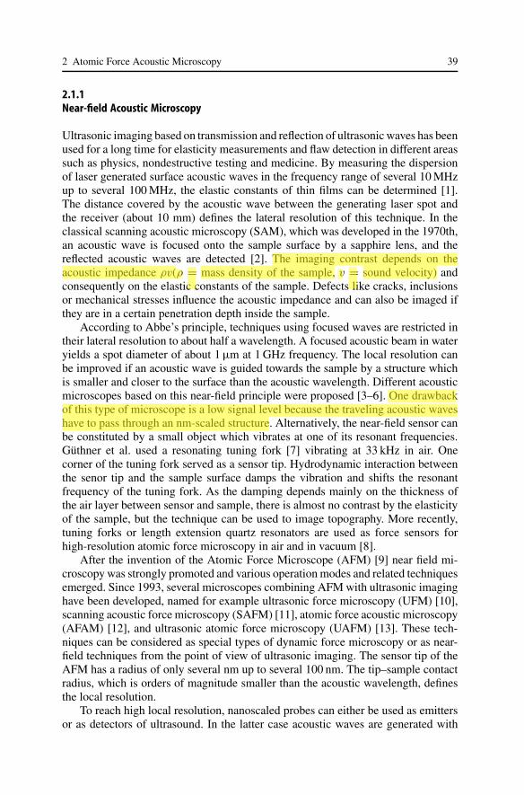
Ultrasonic imaging based on transmission and reflection of ultrasonic waves has beenused for a long time for elasticity measurements and flaw detection in different areassuch as physics, nondestructive testing and medicine. By measuring the dispersionof laser generated surface acoustic waves in the frequency range of several 10 MHzup to several 100 MHz, the elastic constants of thin films can be determined [1].The distance covered by the acoustic wave between the generating laser spot andthe receiver (about 10 mm) defines the lateral resolution of this technique. In theclassical scanning acoustic microscopy (SAM), which was developed in the 1970th,an acoustic wave is focused onto the sample surface by a sapphire lens, and thereflected acoustic waves are detected [2]. The imaging contrast depends on theacoustic impedance ρv(ρ = mass density of the sample, v = sound velocity) andconsequently on the elastic constants of the sample. Defects like cracks, inclusionsor mechanical stresses influence the acoustic impedance and can also be imaged ifthey are in a certain penetration depth inside the sample.

According to Abbe’s principle, techniques using focused waves are restricted intheir lateral resolution to about half a wavelength. A focused acoustic beam in wateryields a spot diameter of about 1 µm at 1 GHz frequency. The local resolution canbe improved if an acoustic wave is guided towards the sample by a structure whichis smaller and closer to the surface than the acoustic wavelength. Different acousticmicroscopes based on this near-field principle were proposed [3–6]. One drawbackof this type of microscope is a low signal level because the traveling acoustic waveshave to pass through an nm-scaled structure. Alternatively, the near-field sensor canbe constituted by a small object which vibrates at one of its resonant frequencies.Güthner et al. used a resonating tuning fork [7] vibrating at 33 kHz in air. Onecorner of the tuning fork served as a sensor tip. Hydrodynamic interaction betweenthe senor tip and the sample surface damps the vibration and shifts the resonantfrequency of the tuning fork. As the damping depends mainly on the thickness ofthe air layer between sensor and sample, there is almost no contrast by the elasticityof the sample, but the technique can be used to image topography. More recently,tuning forks or length extension quartz resonators are used as force sensors forhigh-resolution atomic force microscopy in air and in vacuum [8].

After the invention of the Atomic Force Microscope (AFM) [9] near field mi-croscopy was strongly promoted and various operation modes and related techniquesemerged. Since 1993, several microscopes combining AFM with ultrasonic imaginghave been developed, named for example ultrasonic force microscopy (UFM) [10],scanning acoustic force microscopy (SAFM) [11], atomic force acoustic microscopy(AFAM) [12], and ultrasonic atomic force microscopy (UAFM) [13]. These tech-niques can be considered as special types of dynamic force microscopy or as near-field techniques from the point of view of ultrasonic imaging. The sensor tip of theAFM has a radius of only several nm up to several 100 nm. The tip–sample contactradius, which is orders of magnitude smaller than the acoustic wavelength, definesthe local resolution.

To reach high local resolution, nanoscaled probes can either be used as emittersor as detectors of ultrasound. In the latter case acoustic waves are generated with

40 U. Rabe

conventional ultrasonic transducers, and a scanning probe microscope is used todetect the acoustic wave fields at the sample surface. In atomic force microscopythe tip–sample forces are a nonlinear function of tip–sample distance. The nonlinearforces cause frequency mixing, if an ultrasonic excitation signal is applied to a trans-ducer below the sample and another vibration with a slightly different frequency isexcited in the cantilever and its sensor tip [11, 14]. In the scanning acoustic forcemicroscopy [14] mixing of two surface waves which propagate in different directionis exploited to image surface acoustic wave fields with submicron lateral resolu-tion. Interference phenomena caused by scattering of a plane wave by a disk-shapedstructure were observed in this way [15].

The nonlinearity of the tip–sample forces has a rectifying effect which is ex-ploited in ultrasonic force microscopy [10, 16]. In UFM, an ultrasonic transducergenerating longitudinal waves is placed below the sample. The amplitude of thesinusoidal excitation applied to the transducer is modulated with a saw-tooth sig-nal. The acoustic wave causes a high frequency out-of-plane surface vibration witha low-frequency amplitude modulation. The sensor tip of the AFM is in contact withthe vibrating sample surface and when the threshold amplitude is reached, the sensortip lifts off from the surface. A lock-in amplifier which operates at the modulationfrequency detects the envelope of the high frequency signal. This rectifying propertywas called “mechanical diode effect”. A qualitative image of elastic sample prop-erties and contrast from subsurface objects can be obtained [16–18]. A rectifyingeffect due to the nonlinear forces is also observed when the amplitude modulatedvibration is excited at the fixed end of the cantilever (“waveguide UFM”) [19]. Thecontrast in UFM was examined by different research groups [20,21]. The advantageof the mixing technique and the UFM is the low bandwidth which is required for theposition detector in the AFM. Because the modulation frequency can be chosen inthe kHz range, a direct detection of signals at MHz or even GHz frequencies is notnecessary. As both, elasticity and adhesion, contribute to the image contrast [22], itis difficult to separate surface elasticity quantitatively from adhesion.

2.1.2Scanning Probe Techniques and Nanoindentation

Different dynamic operation modes of the scanning force microscope were suggestedto measure elasticity on an nm scale. In the force-modulation mode (FMM) the sen-sor tip is in contact with the probed surface, and the surface is vibrated normally orlaterally at a frequency below the first resonance of the cantilever [23]. The amplitudeor phase of the vibration of the cantilever is evaluated. Force modulation microscopyprovides elasticity contrast of softer samples like for example polymers. If stiffer ma-terials like metals and ceramics are to be examined, the contact stiffness between tipand surface becomes much higher than the spring constant of the cantilever (0.1 N/mup to several 10 N/m, depending on the type of beam) and the contrast decreases.Instead of applying the force indirectly by varying the distance between the surfaceand the fixed end of the cantilever, other research groups applied a magnetic forcedirectly to the cantilever [24,25]. Some authors extend force-modulation microscopyto the higher modes of the cantilever [25–27]. Here, this type of operation is calledcontact-resonance spectroscopy and will be treated in detail in the next paragraphs.

2 Atomic Force Acoustic Microscopy 41

In the pulsed force mode [28] the distance between the fixed end of the sensor andthe sample surface is also modulated at a frequency below the resonant frequenciesof the sensor. The amplitude is so high (10–500 nm) that the tip loses contact withthe sample surface during its vibration cycle. Characteristic points in the vibrationsignal of the cantilever are evaluated to image elasticity and adhesion. In scanninglocal acceleration microscopy (SLAM) the sensor tip is in contact with a samplesurface that is vibrated out-of-plane with a frequency slightly above the first flexuralresonance of the cantilever [29]. Using a temperature controlled SLAM instrument,Oulevey et al. observed martensitic phase transformation in NiTi-alloy [30].

Force-modulation microscopy can be considered as direct detection of low fre-quency acoustical vibrations by an AFM. A sensor tip which touches the samplesurface during its vibration cycle for example in FMM or tapping mode [31] radiatessound into the sample, but the amplitudes are usually below the detection limit ofcommercial transducers [32]. If the sensor of the AFM is magnified by only oneor two orders of magnitude like in scanning microdeformation microscopy (SMM),the acoustical amplitudes transmitted through the sample become detectable [33].Subsurface features were imaged by SMM in transmission mode [34]. The vibrationof the cantilever was measured with a piezoelectric element [35] or with an opticalinterferometer pointing onto the cantilever [36]. The AFM sensor and the SMMcantilever are so similar to each other that many aspects of the equation of motionand the contact mechanics models are identical. As the radius of the SMM sensor tipis larger than the radius of an AFM tip the tip–sample interaction is easier to controland macroscopic contact models are easier to apply. Because the contact area scaleswith the size of the sensor tip, the lateral resolution is lower in SMM than in theAFM based techniques.

Nanoindentation, which was originally developed to measure hardness, can alsobe used for elasticity measurements [37]. In dynamic nanoindentation a low ampli-tude sinusoidal force modulation is superimposed to the quasi static load applied tothe indenter. Amplitude and phase of the vibration of the electromechanical system,constituted by the indenter and the force detection unit, are evaluated to measurecontact stiffness as a function of load [38]. The indenter tips are of Berkovich typemade of diamond or spherical with a radius of 100 µm. The local resolution of thenanoindenter is typically 100 nm to 200 nm because of the mechanical stress field inthe sample at a minimum penetration depth of about 20 nm. Seyed Asif et al. imagedthe real and imaginary parts of the Young’s modulus of carbon fibers in epoxy matrixby dynamic nanoindentation [39]. Especially for examination of softer materials likepolymers, dynamic nanoindentation became very popular during the last years. Anoverview of commercial instruments can be found for example in a publication byBushan and Li [40].

2.1.3Vibration Modes of AFM Cantilevers

The typical dimensions of cantilevers for atomic force microscopy are several 100 µmin length, several 10 µm in width and several 100 nm up to several µm in thickness.The sensors are small plates or beams having distributed mass, and they can beexcited to different modes of vibration such as flexural or torsional modes. While

42 U. Rabe

most of the dynamic scanning probe applications relied on the fundamental modesof the beams, for noise analysis the importance of the higher eigenmodes wasrecognized by different authors [41, 42]. In atomic force acoustic microscopy andultrasonic atomic force microscopy the flexural resonant frequencies of atomic forcemicroscope cantilevers are measured [13, 43, 44]. The sensor of the AFM can beconsidered as a cantilever beam which is clamped at one end and free at the otherend. If the sensor tip is in contact with a sample surface tip–sample interaction forceschange the end conditions and all resonant frequencies of the cantilever are shifted.Furthermore, tip–sample interaction causes damping and changes the width of theresonance curves.

When the cantilever is in flexural vibration, a large component of the amplitudeof the tip apex is normal to the sample surface. Therefore flexural modes are used tomeasure normal tip–sample contact stiffness, which in turn depends on the Young’smodulus of tip and sample, on the shear modulus of tip and sample, on the contactarea, and on the adhesion forces. In most cases, the flexural modes cause an angularoscillation of the cantilever beam at the position where the tip is fixed, which inturn leads to an oscillation of the tip apex parallel to the surface. This means thatthe flexural modes are also influenced by lateral tip–sample contact stiffness andfriction.

Torsion of AFM cantilevers is used to measure lateral forces and friction [45,46]and a variety of dynamic operation modes exploiting torsional vibration is known.Similar to AFAM and UAFM the torsional resonant frequency and the width of theresonant peaks can be determined to measure in-plane surface properties [47,48]. Atlow amplitudes the sensor tip sticks to the sample surface, and at higher amplitudessliding sets in. The stick-slip events cause a characteristic plateau in the shapeof the contact-resonance curves [49]. Torsional modes are not the only type ofvibration exhibiting a strong component of lateral tip–sample amplitude. Bendingof the cantilever in its thickness direction leads to non-negligible lateral tip–sampledisplacement [50], and lateral bending modes of the cantilever can be used forimaging and spectroscopy [51]. In the so-called “overtone atomic force microscopy”Drobeck et al. exploited the torsional vibration modes of V -shaped cantileversto measure in-plane surface stiffness [52, 53]. Elasticity contrast was obtained onAl−Ni−Fe quasicrystal samples [52], and the lateral stiffness of Si, Al, and CdTesurfaces was evaluated quantitatively [53]. The results were obtained in ambientconditions by analysis of the thermal noise of the cantilevers.

2.2Linear Contact-resonance Spectroscopy Using Flexural Modes

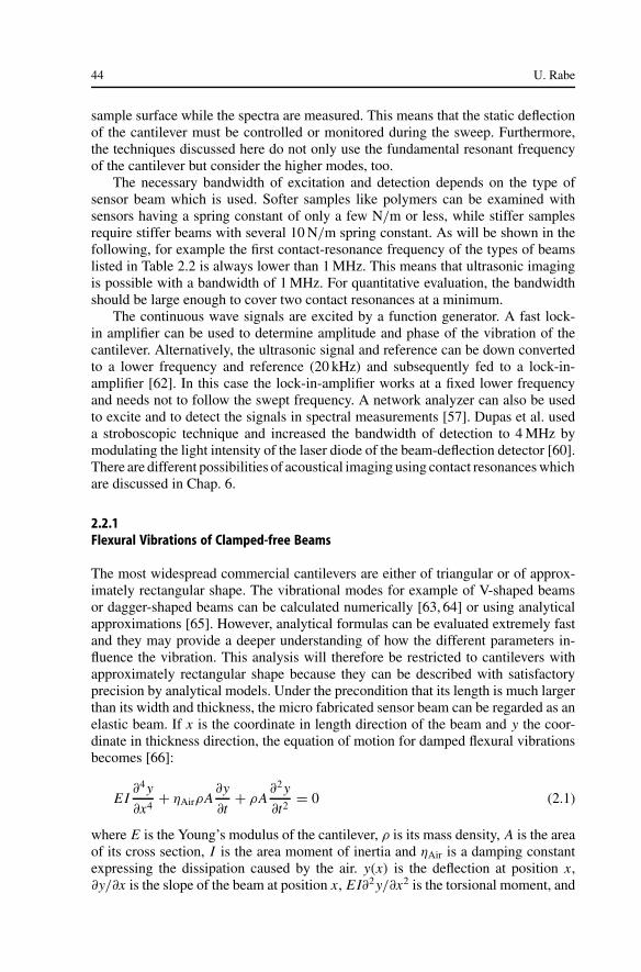
Contact-resonance spectroscopy techniques which exploit the flexural modes of thecantilevers can be organized according to the method of excitation. In the AFAM-technique a transducer below the sample excites longitudinal waves which cause out-of-plane vibrations of the investigated surface (transducer 1 in Fig. 2.1) [43,44]. Viathe tip–sample contact forces the vibrations are transmitted into the cantilever. Theflexural vibrations can also be excited by a transducer which generates oscillations ofthe fixed end of the beam (transducer 2 in Fig. 2.1). This technique (UAFM) was first

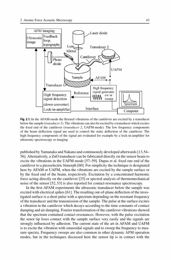
2 Atomic Force Acoustic Microscopy 43

Fig. 2.1. In the AFAM-mode the flexural vibrations of the cantilever are excited by a transducerbelow the sample (transducer 1). The vibrations can also be excited by a transducer which excitesthe fixed end of the cantilever (transducer 2, UAFM-mode). The low frequency componentsof the beam deflection signal are used to control the static deflection of the cantilever. Thehigh frequency components of the signal are evaluated for example by a lock-in-amplifier forultrasonic spectroscopy or imaging

published by Yamanaka and Nakano and continuously developed afterwards [13,54–56]. Alternatively, a ZnO transducer can be fabricated directly on the sensor beam toexcite the vibrations in the UAFM-mode [57–59]. Dupas et al. fixed one end of thecantilever to a piezoelectric bimorph [60]. For simplicity the technique is designatedhere by AFAM or UAFM, when the vibrations are excited by the sample surface orby the fixed end of the beam, respectively. Excitation by a concentrated harmonicforce acting directly on the cantilever [25] or spectral analysis of thermomechanicalnoise of the sensor [52, 53] is also reported for contact-resonance spectroscopy.

In the first AFAM experiments the ultrasonic transducer below the sample wasexcited with electrical spikes [61]. The resulting out-of-plane deflection of the inves-tigated surface is a short pulse with a spectrum depending on the resonant frequencyof the transducer and the transmission of the sample. The pulse at the surface excitesa vibration in the cantilever which decays according to the time constants of contactdamping and air damping. Fourier transformation of the cantilever vibrations showedthat the spectrum contained contact resonances. However, with the pulse excitationthe senor tip loses contact with the sample surface very easily and the signals arestrongly influenced by adhesion. The current state of the art in AFAM and UAFMis to excite the vibration with sinusoidal signals and to sweep the frequency to mea-sure spectra. Frequency sweeps are also common in other dynamic AFM operationmodes, but in the techniques discussed here the sensor tip is in contact with the

44 U. Rabe

sample surface while the spectra are measured. This means that the static deflectionof the cantilever must be controlled or monitored during the sweep. Furthermore,the techniques discussed here do not only use the fundamental resonant frequencyof the cantilever but consider the higher modes, too.

The necessary bandwidth of excitation and detection depends on the type ofsensor beam which is used. Softer samples like polymers can be examined withsensors having a spring constant of only a few N/m or less, while stiffer samplesrequire stiffer beams with several 10 N/m spring constant. As will be shown in thefollowing, for example the first contact-resonance frequency of the types of beamslisted in Table 2.2 is always lower than 1 MHz. This means that ultrasonic imagingis possible with a bandwidth of 1 MHz. For quantitative evaluation, the bandwidthshould be large enough to cover two contact resonances at a minimum.

The continuous wave signals are excited by a function generator. A fast lock-in amplifier can be used to determine amplitude and phase of the vibration of thecantilever. Alternatively, the ultrasonic signal and reference can be down convertedto a lower frequency and reference (20 kHz) and subsequently fed to a lock-in-amplifier [62]. In this case the lock-in-amplifier works at a fixed lower frequencyand needs not to follow the swept frequency. A network analyzer can also be usedto excite and to detect the signals in spectral measurements [57]. Dupas et al. useda stroboscopic technique and increased the bandwidth of detection to 4 MHz bymodulating the light intensity of the laser diode of the beam-deflection detector [60].There are different possibilities of acoustical imaging using contact resonances whichare discussed in Chap. 6.

2.2.1Flexural Vibrations of Clamped-free Beams

The most widespread commercial cantilevers are either of triangular or of approx-imately rectangular shape. The vibrational modes for example of V-shaped beamsor dagger-shaped beams can be calculated numerically [63, 64] or using analyticalapproximations [65]. However, analytical formulas can be evaluated extremely fastand they may provide a deeper understanding of how the different parameters in-fluence the vibration. This analysis will therefore be restricted to cantilevers withapproximately rectangular shape because they can be described with satisfactoryprecision by analytical models. Under the precondition that its length is much largerthan its width and thickness, the micro fabricated sensor beam can be regarded as anelastic beam. If x is the coordinate in length direction of the beam and y the coor-dinate in thickness direction, the equation of motion for damped flexural vibrationsbecomes [66]:

EI∂4 y

∂x4+ ηAirρA

∂y

∂t+ ρA

∂2 y

∂t2= 0 (2.1)

where E is the Young’s modulus of the cantilever, ρ is its mass density, A is the areaof its cross section, I is the area moment of inertia and ηAir is a damping constantexpressing the dissipation caused by the air. y(x) is the deflection at position x,∂y/∂x is the slope of the beam at position x, EI∂2 y/∂x2 is the torsional moment, and

2 Atomic Force Acoustic Microscopy 45

EI∂3 y/∂x3 is the shear force. One seeks a harmonic solution in time with angularfrequency ω = 2π f . The solution of the differential equation of motion may bewritten:

y(x, t) = y(x) · y(t) = (a1 eαx + a2 e−αx + a3 eiαx + a4 e−iαx) eiωt . (2.2)

The mode shape y(x) can also be expressed as:

y(x) = A1(cos αx + cosh αx) + A2(cos αx − cosh αx)

+ A3(sin αx + sinh αx) + A4(sin αx − sinh αx) , (2.3)

where a1, a2, a3, a4 and A1, A2, A3, A4 are constants. By substituting the solution(2.2) in the equation of motion (2.1) one obtains the dispersion relation for a flexuralwave with complex wave number α:

EIα4 + iρAηAirω − ρAω2 = 0 (2.4)

α± = ± 4

√ρA

EI(ω2 ∓ iηAirω) . (2.5)

In absence of damping the dispersion equation simplifies to:

f = (αL)2

2π

1

L2

√EI

ρA. (2.6)

Boundary conditions must be fulfilled if the beam is of finite length L. Bysubstituting the boundary conditions in the general solution one obtains a charac-teristic equation. For a beam with one clamped end and one free end one finds intextbooks [66, 67]:

cos αL cosh αL + 1 = 0 (2.7)

The roots αn L of this equation can be calculated numerically, where n =1, 2, 3, . . . is the mode number. Examples are listed in Table 2.1. Using the disper-sion relation one obtains the resonant frequencies of the beam. The quality factor Qof the resonances is given by:

Q = ωn

∆ω= ωn

ηAir(2.8)

According to (2.8), the quality factor Q increases with the mode number. Ex-perimentally one often observes an increase in Q for the first modes up to 1 MHzfollowed by a decrease at still higher frequencies [44]. This means that the dampingηAir is in fact a function of the frequency. Quality factors of the first flexural reso-nances of commercial sensors in air are typically between Q = 200 and Q = 900for sensors made of single crystal silicon.

With most commercial atomic force microscopes the cantilever can be excited toforced vibration when its one end is free. The fundamental mode of the clamped-freebeam and the quality factor of the resonance can be measured in this way. On the

46 U. Rabe

Table 2.1. Dimensionless wave number αn L and frequency ratio fn/ f1,free for different boundaryconditions of the beam: clamped-free ( fn,free), clamped-pinned ( fn,pin), and clamped-clamped( fn,clamp)

n (αn L)free fn,free/ f1,free (αn L)pin fn,pin/ f1,free (αn L)clamp fn,clamp/ f1,free

1 1.87510 1.00 3.92660 4.39 4.73004 6.362 4.69409 6.27 7.06858 14.21 7.85320 17.543 7.85476 17.55 10.21018 29.65 10.99561 34.394 10.99554 34.39 13.35177 50.70 14.13717 56.845 14.13717 56.84 16.49336 77.37 17.27876 84.916 17.27876 84.91 19.63495 109.65 20.42035 118.607 20.42035 118.60 22.77655 147.55 23.56194 157.90

≈ 2n−12 π ≈ 4n+1

4 π ≈ 2n+12 π

other hand, the constants ρ, A, E, I , and ηAir are often unknown. It is therefore betterto rewrite the dispersion relations (2.5) and (2.6) in terms of measurable quantities:

α±L = ±α1,freeL · 4

√ω2

ω21,free

∓ iηAirω

ω21,free

≈ ±1.8751 · 4

√(f

f1,free

)2

∓ i1

Q1,free

f

f1,free(2.9)

f

f1,free= (αL)2(

α1,freeL)2 . (2.10)

Due to the high quality factors Q of the flexural modes in air the shift ofthe resonant frequencies caused by air damping is negligible. Here the resonantfrequencies of the clamped-free beam are sometimes called “free” resonances. Inthis case “free vibration” is not meant as the opposite of “forced vibration” butrelates to the end condition of the beam. The theory predicts a certain ratio of thefree flexural resonant frequencies regardless of the cross section and the length ofthe beam, for example:

f2,free

f1,free= (4.6941)2

(1.8751)2 = 6.27 . (2.11)

The first ten solutions αn L for the clamped-free beam without damping(ηAir = 0) are listed in Table 2.1. Note that the bending modes are not equidis-tant in frequency. According to the dispersion equation, the frequency ω is notproportional to the wave number α, but ω ∼ α2. For the higher modes the fre-quency interval to the next higher mode increases with the square of the fre-quency. The higher bending modes are no harmonics of the fundamental fre-quency.

2 Atomic Force Acoustic Microscopy 47

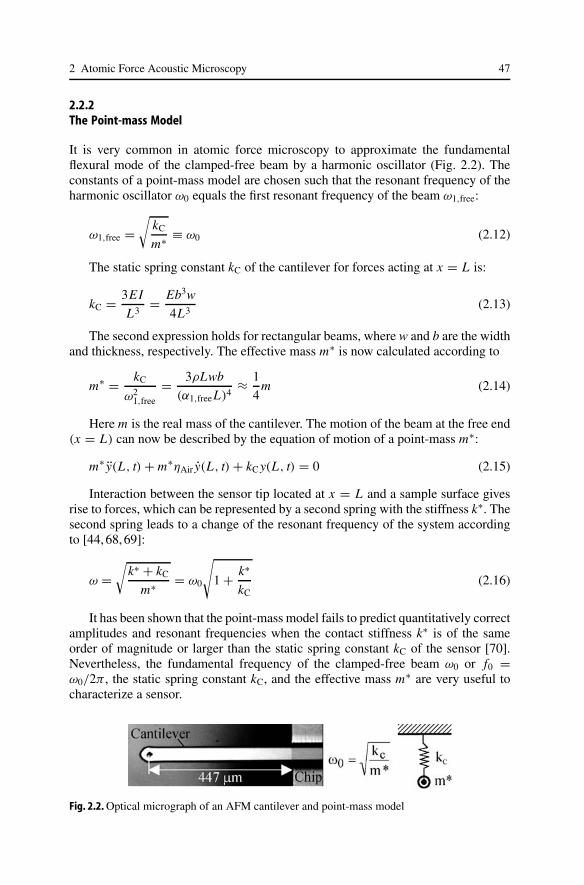
2.2.2The Point-mass Model

It is very common in atomic force microscopy to approximate the fundamentalflexural mode of the clamped-free beam by a harmonic oscillator (Fig. 2.2). Theconstants of a point-mass model are chosen such that the resonant frequency of theharmonic oscillator ω0 equals the first resonant frequency of the beam ω1,free:

ω1,free =√

kC

m∗ ≡ ω0 (2.12)

The static spring constant kC of the cantilever for forces acting at x = L is:

kC = 3EI

L3= Eb3w

4L3(2.13)

The second expression holds for rectangular beams, where w and b are the widthand thickness, respectively. The effective mass m∗ is now calculated according to

m∗ = kC

ω21,free

= 3ρLwb

(α1,freeL)4≈ 1

4m (2.14)

Here m is the real mass of the cantilever. The motion of the beam at the free end(x = L) can now be described by the equation of motion of a point-mass m∗:

m∗ y(L, t) + m∗ηAir y(L, t) + kC y(L, t) = 0 (2.15)

Interaction between the sensor tip located at x = L and a sample surface givesrise to forces, which can be represented by a second spring with the stiffness k∗. Thesecond spring leads to a change of the resonant frequency of the system accordingto [44, 68, 69]:

ω =√

k∗ + kC

m∗ = ω0

√1 + k∗

kC(2.16)

It has been shown that the point-mass model fails to predict quantitatively correctamplitudes and resonant frequencies when the contact stiffness k∗ is of the sameorder of magnitude or larger than the static spring constant kC of the sensor [70].Nevertheless, the fundamental frequency of the clamped-free beam ω0 or f0 =ω0/2π, the static spring constant kC, and the effective mass m∗ are very useful tocharacterize a sensor.

Fig. 2.2. Optical micrograph of an AFM cantilever and point-mass model

48 U. Rabe

2.2.3Experiments with Clamped-free Beams

With respect to application it is important to examine how well real sensors corre-spond to the flexural beam model. It is helpful to use a calibrated optical interfer-ometer with a bandwidth of several MHz to examine as many of the higher modesof the cantilever as possible [44, 71]. For example, Hoummady et al. examinedhigher flexural modes of AFM cantilevers interferometrically in order to use themfor imaging [72] and Cretin and Vairac used an optical interferometer to measurethe vibration of the sensor in SMM [36].

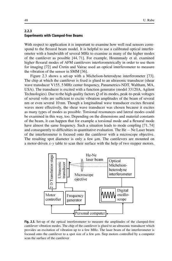
Figure 2.3 shows a set-up with a Michelson-heterodyne interferometer [73].The chip at which the cantilever is fixed is glued to an ultrasonic transducer (shearwave transducer V155, 5 MHz center frequency, Panametrics-NDT, Waltham, MA,USA). The transducer is excited with a function generator (model 33120A, AgilentTechnologies). Due to the high quality factors Q of its modes, peak-to-peak voltagesof several volts are sufficient to excite vibration amplitudes of the beam of severalnm or even several 10 nm. Though a longitudinal wave transducer excites flexuralwaves more effectively, the shear wave transducer was chosen because it excitesas many types of modes as possible. Torsional resonances and lateral modes couldbe examined in this way, too. Depending on the dimensions and material constantsof the beam, it can happen that for example a torsional mode and a flexural modehave almost the same frequency. Such a situation leads to mode coupling [71, 74]and consequently to difficulties in quantitative evaluation. The He − Ne Laser beamof the interferometer is focused onto the cantilever with a microscope objective.The resulting spot diameter is only a few µm. The cantilevers are mounted ona motor-driven x-y table to scan their surface with the help of two stepper motors.

Fig. 2.3. Set-up of the optical interferometer to measure the amplitudes of the clamped-freecantilever vibration modes. The chip of the cantilever is glued to an ultrasonic transducer whichprovides an excitation of vibration up to a few MHz. The laser beam of the interferometer isfocused onto the cantilever to a spot size of a few µm. Step motors controlled by a computerscan the surface of the cantilever

2 Atomic Force Acoustic Microscopy 49

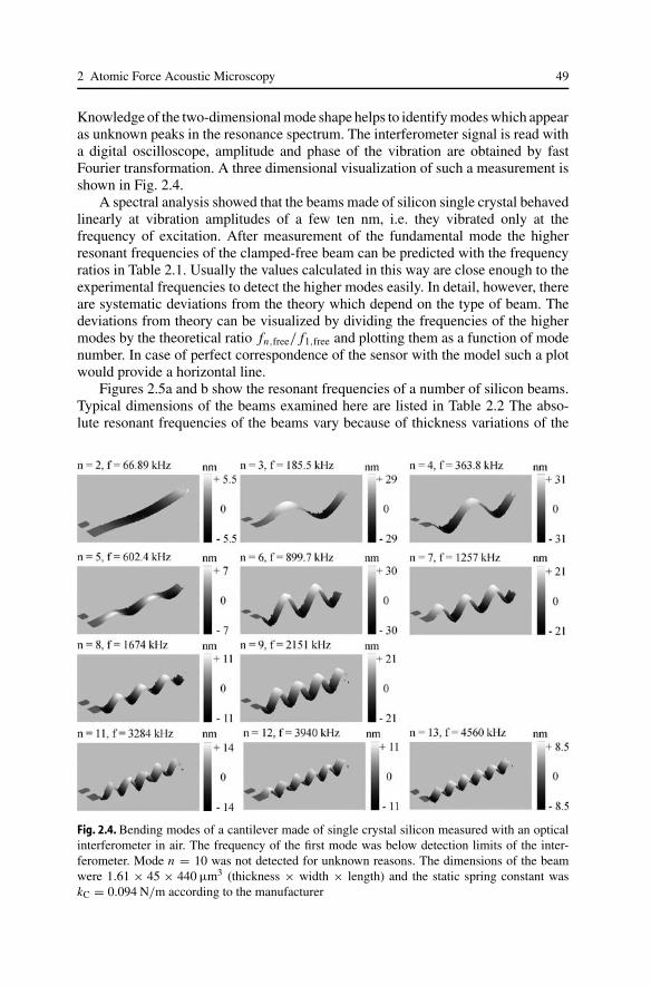
Knowledge of the two-dimensional mode shape helps to identify modes which appearas unknown peaks in the resonance spectrum. The interferometer signal is read witha digital oscilloscope, amplitude and phase of the vibration are obtained by fastFourier transformation. A three dimensional visualization of such a measurement isshown in Fig. 2.4.

A spectral analysis showed that the beams made of silicon single crystal behavedlinearly at vibration amplitudes of a few ten nm, i.e. they vibrated only at thefrequency of excitation. After measurement of the fundamental mode the higherresonant frequencies of the clamped-free beam can be predicted with the frequencyratios in Table 2.1. Usually the values calculated in this way are close enough to theexperimental frequencies to detect the higher modes easily. In detail, however, thereare systematic deviations from the theory which depend on the type of beam. Thedeviations from theory can be visualized by dividing the frequencies of the highermodes by the theoretical ratio fn,free/ f1,free and plotting them as a function of modenumber. In case of perfect correspondence of the sensor with the model such a plotwould provide a horizontal line.

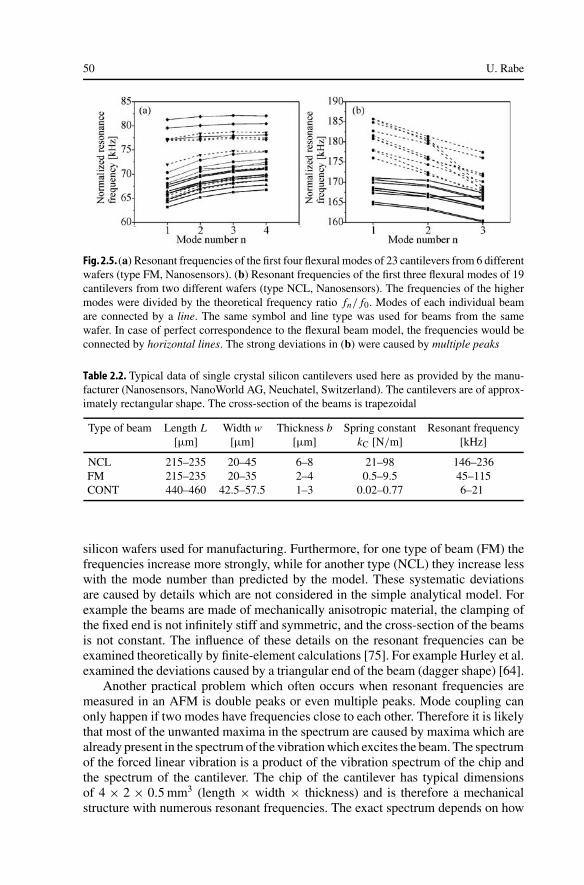
Figures 2.5a and b show the resonant frequencies of a number of silicon beams.Typical dimensions of the beams examined here are listed in Table 2.2 The abso-lute resonant frequencies of the beams vary because of thickness variations of the

Fig. 2.4. Bending modes of a cantilever made of single crystal silicon measured with an opticalinterferometer in air. The frequency of the first mode was below detection limits of the inter-ferometer. Mode n = 10 was not detected for unknown reasons. The dimensions of the beamwere 1.61 × 45 × 440 µm3 (thickness × width × length) and the static spring constant waskC = 0.094 N/m according to the manufacturer

50 U. Rabe

Fig. 2.5. (a) Resonant frequencies of the first four flexural modes of 23 cantilevers from 6 differentwafers (type FM, Nanosensors). (b) Resonant frequencies of the first three flexural modes of 19cantilevers from two different wafers (type NCL, Nanosensors). The frequencies of the highermodes were divided by the theoretical frequency ratio fn/ f0. Modes of each individual beamare connected by a line. The same symbol and line type was used for beams from the samewafer. In case of perfect correspondence to the flexural beam model, the frequencies would beconnected by horizontal lines. The strong deviations in (b) were caused by multiple peaks

Table 2.2. Typical data of single crystal silicon cantilevers used here as provided by the manu-facturer (Nanosensors, NanoWorld AG, Neuchatel, Switzerland). The cantilevers are of approx-imately rectangular shape. The cross-section of the beams is trapezoidal

Type of beam Length L Width w Thickness b Spring constant Resonant frequency[µm] [µm] [µm] kC [N/m] [kHz]

NCL 215–235 20–45 6–8 21–98 146–236FM 215–235 20–35 2–4 0.5–9.5 45–115CONT 440–460 42.5–57.5 1–3 0.02–0.77 6–21

silicon wafers used for manufacturing. Furthermore, for one type of beam (FM) thefrequencies increase more strongly, while for another type (NCL) they increase lesswith the mode number than predicted by the model. These systematic deviationsare caused by details which are not considered in the simple analytical model. Forexample the beams are made of mechanically anisotropic material, the clamping ofthe fixed end is not infinitely stiff and symmetric, and the cross-section of the beamsis not constant. The influence of these details on the resonant frequencies can beexamined theoretically by finite-element calculations [75]. For example Hurley et al.examined the deviations caused by a triangular end of the beam (dagger shape) [64].

Another practical problem which often occurs when resonant frequencies aremeasured in an AFM is double peaks or even multiple peaks. Mode coupling canonly happen if two modes have frequencies close to each other. Therefore it is likelythat most of the unwanted maxima in the spectrum are caused by maxima which arealready present in the spectrum of the vibration which excites the beam. The spectrumof the forced linear vibration is a product of the vibration spectrum of the chip andthe spectrum of the cantilever. The chip of the cantilever has typical dimensionsof 4 × 2 × 0.5 mm3 (length × width × thickness) and is therefore a mechanicalstructure with numerous resonant frequencies. The exact spectrum depends on how

2 Atomic Force Acoustic Microscopy 51

the chip is clamped [75]. In the AFAM-mode ultrasonic waves transmitted througha sample generate the surface vibration, which means that in this case the spectrumof the exciting signal depends on the material, the dimensions, and the clamping ofthe sample.

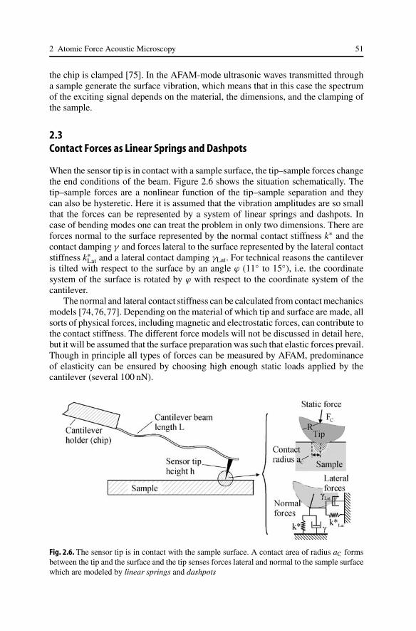
2.3Contact Forces as Linear Springs and Dashpots

When the sensor tip is in contact with a sample surface, the tip–sample forces changethe end conditions of the beam. Figure 2.6 shows the situation schematically. Thetip–sample forces are a nonlinear function of the tip–sample separation and theycan also be hysteretic. Here it is assumed that the vibration amplitudes are so smallthat the forces can be represented by a system of linear springs and dashpots. Incase of bending modes one can treat the problem in only two dimensions. There areforces normal to the surface represented by the normal contact stiffness k∗ and thecontact damping γ and forces lateral to the surface represented by the lateral contactstiffness k∗

Lat and a lateral contact damping γLat. For technical reasons the cantileveris tilted with respect to the surface by an angle ϕ (11 to 15), i.e. the coordinatesystem of the surface is rotated by ϕ with respect to the coordinate system of thecantilever.

The normal and lateral contact stiffness can be calculated from contact mechanicsmodels [74,76,77]. Depending on the material of which tip and surface are made, allsorts of physical forces, including magnetic and electrostatic forces, can contribute tothe contact stiffness. The different force models will not be discussed in detail here,but it will be assumed that the surface preparation was such that elastic forces prevail.Though in principle all types of forces can be measured by AFAM, predominanceof elasticity can be ensured by choosing high enough static loads applied by thecantilever (several 100 nN).

Fig. 2.6. The sensor tip is in contact with the sample surface. A contact area of radius aC formsbetween the tip and the surface and the tip senses forces lateral and normal to the sample surfacewhich are modeled by linear springs and dashpots

52 U. Rabe

The Hertzian model describes the contact between two nonconforming elasticbodies of general anisotropy [78]. In the simplest case the bodies are mechanicallyisotropic, the sample is considered as flat and the sensor tip is represented bya sphere with a radius R. If a normal force Fn acts onto the sphere, a contact radiusaC forms:

aC = 3√

3Fn R/4E∗ . (2.17)

If the adhesion forces are so small that they can be neglected, the normal force Fn

is given by the static deflection of the cantilever multiplied with the spring constantof the cantilever. The sum of the indentation in the contacting bodies, δn, i.e. theamount the two bodies approach is given by:

δn = 3

√9F2

n

16RE∗2, (2.18)

The normal contact stiffness k∗ is:

k∗ = 2aC E∗ = 3√

6E∗2 RFn . (2.19)

Here, E∗ is the reduced Young’s modulus of the contact which is given by

1

E∗ =(1 − ν2

S

)ES

+(1 − ν2

T

)ET

, (2.20)

where ES, ET, νS, νT, are Young’s modulus and Poisson’s ratio of the surfaceand the tip, respectively. After AFAM experiments, the tip shape often deviatesfrom that of a sphere [79]. In this case the shape of the tip can be described moregenerally by a body of revolution. It has been shown that for axisymmetric indenterson elastically isotropic half spaces the contact stiffness k∗, i.e. the derivative ofthe applied load Fn with respect to the indention depth, δn , generally obeys theequation [80]:

k∗ = dFn

dδn= 2√

π

√SE∗ (2.21)

Here S = π × a2C is the contact area. Therefore the relation

E∗ = k∗/(2aC) , (2.22)

which can be derived from the Hertzian model, still holds in this more general case.These formulas are derived on the assumptions of a frictionless contact. The Hertzianmodel is only valid if the contact area is small compared with the dimensions ofthe contacting bodies and their radii of curvature [78], which means that the contactradius must be smaller than the tip radius aC R. Linear elastic theory is only validif the mechanical stresses remain small enough. In AFM these two conditions areeasily violated when a sensor tip with a radius of a few nm contacts a metallic orceramic sample surface.

2 Atomic Force Acoustic Microscopy 53

The contact radius defines the lateral resolution in contact-resonance spec-troscopy. A typical contact radius in AFM ranges from several nm up to severaltens of nanometers, depending on the tip radius and the elasticity of the tip andthe sample. Many polycrystalline materials like metals and ceramics, which appearmechanically homogeneous on a macroscopic scale, show a local variation in elasticconstants for a scanning probe microscope because the tip senses the individualgrains within the polycrystalline aggregate. Each grain represents a small singlecrystal. This means that imaging by AFAM can only be explained when the samplesurface is no longer treated as an isotropic material. Furthermore AFM sensor tipsmade of single crystalline silicon are not elastically isotropic, and this holds for othertip materials as well. Mechanically anisotropic materials are described by more thantwo elastic constants. In the most general case of two non-conforming bodies of gen-eral shape and anisotropy, the contact area is elliptical [78]. The reduced Young’smodulus of the contact is a function of the indentation δn, contains combinationsof the elastic constants of tip and sample and cannot be separated into a sum ofa contribution from tip and surface like in (2.20). Vlassak and Nix examined theindentation of a rigid parabolic punch in an anisotropic surface [81]. They showedthat the contact area remains spherical if a three- or fourfold rotational symmetryaxis perpendicular to the boundary exists. In this case (2.19) and (2.21) remain validif the isotropic reduced elastic modulus E/(1 − ν2) is replaced by an indentationmodulus that is calculated numerically from single crystal elastic constants [82].Equation (2.20) is replaced by:

1

E∗ = 1

MS+ 1

MT(2.23)

where MS and MT are the indentation modulus of the sample and the tip, respectively.The required symmetry holds for silicon sensor tips which are oriented in (001)crystallographic direction. Because of its fourfold symmetry the tip does not alterthe rotational symmetry if it is in vertical contact with an isotropic body or witha sample which also has a fourfold rotational symmetry axis along the tip andindentation axis. Even for bodies which do not have a three- or fourfold symmetryaxis (2.23) can be used as a first approximation. The error made by application ofthis equation depends on the anisotropy and can be estimated [83].

The tilt angle ϕ of the cantilever causes tip–sample forces tangential to the sur-face when the surface is moved in its normal direction. Additionally, the flexuralvibrations cause an angular deflection ∂y/∂x at the sensor-tip position and conse-quently a lateral deflection h∂y/∂x of the sensor tip apex. Tangential forces weretreated by Mindlin [78]. The lateral contact stiffness depends on the effective shearstiffness G∗ of the contact:

k∗Lat = dFL

dδL= 8aCG∗ (2.24)

1

G∗ = 2 − νS

GS+ 2 − νT

GT(2.25)

where δL is the lateral contact deflection, and GS and GT are the shear modulusof the sample and the tip, respectively. For isotropic bodies the ratio between thenormal contact stiffness k∗ and the lateral contact stiffness k∗

Lat is independent of the

54 U. Rabe

normal force Fn:

k∗Lat

k∗ = 8aCG∗

2aC E∗ = 4G∗

E∗ . (2.26)

As Mazeran and Loubet pointed out [25], for ET ES

k∗Lat

k∗ ≈ 2(1 − νS)

2 − νS. (2.27)

Taking a range of Poisson’s ratio from 0.1 for diamond to 0.5 for rubber, the ratioof lateral and normal contact stiffness k∗

Lat/k∗ varies from 2/3 to 18/19 with anaverage value of 0.85 [25]. Like in the case of the normal contact stiffness, it will benecessary in future to calculate shear stiffness, taking into account the mechanicalanisotropy of the contacting bodies.

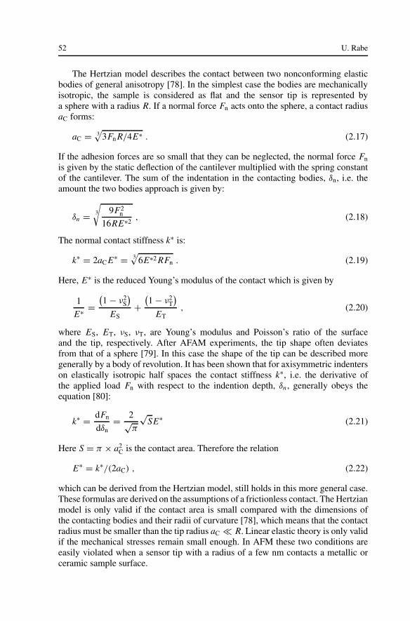
An important question for nondestructive testing is whether techniques likeAFAM or UAFM are able to detect sub-surface features. The typical frequency fof ultrasonic excitation is 100 kHz to 10 MHz. The velocity of longitudinal acousticwaves in the solids under examination ranges typically from v = 1 mm/µs (poly-mers) to v = 10 mm/µs (ceramics). In this case the acoustic wavelength λ = v/ franges from 100 µm to 10 cm. Consequently the acoustic wavelength is larger thanthe scan width of the AFM and orders of magnitude larger than the contact radius.This confirms that the vibrating tip can be seen like a dynamic indenter and the pen-etration depth of the ultrasonic techniques is given by the decay of the mechanicalstress field in the sample.

According to the Hertzian contact model the decay length is several multiplesof the contact radius (see Fig. 2.7). Therefore it is possible to measure the filmthickness with AFAM or UAFM [57], provided the films are thin enough. Yaraliogluet al. calculated the contact stiffness of layered materials using the impedance ofa mechanical radiator [58]. They examined thin films of photo resist, W, Al, andCu on silicon single crystal. They were able to show that in the low frequencylimit ( f → 0) the impedance method provides the same results for the contactstiffness k∗ as the Hertzian contact model and that this method is well suited to

Fig. 2.7. Mechanical stress field in a Hertzian contact as a function of penetration depth z into thesurface. The average normal pressure pn in the contact area is given by pn = Fn/πa2

C, where Fnis the normal force and aC is the contact radius. The compressional stresses σz and σr have theirmaximum at the surface and the principal shear stress τ1 reaches its maximum in the sample [78]

2 Atomic Force Acoustic Microscopy 55

calculate the influence of subsurface defects on the contact stiffness [84]. Tsujiet al. observed subsurface dislocation movement in graphite with UAFM. Theycalculated the influence of a subsurface layer with lower Young’s modulus on thecontact stiffness using finite elements [85–88]. The penetration depth of the me-chanical stress field can be enhanced by increasing the contact radius, however,this causes a loss in lateral resolution. According to Fig. 2.7 the compressionalstress has its maximum at the sample surface, while the shear stress reaches itsmaximum below the surface. Therefore techniques which exploit lateral vibrationslike torsional contact-resonance spectroscopy should be very sensitive to subsurfacedefects.

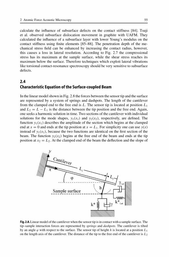
2.4Characteristic Equation of the Surface-coupled Beam

In the linear model shown in Fig. 2.8 the forces between the sensor tip and the surfaceare represented by a system of springs and dashpots. The length of the cantileverfrom the clamped end to the free end is L. The sensor tip is located at position L1

and L2 = L − L1 is the distance between the tip position and the free end. Again,one seeks a harmonic solution in time. Two sections of the cantilever with individualsolutions for the mode shapes, y1(x1) and y2(x2), respectively, are defined. Thefunction y1(x1) describes the amplitude of the section which begins at the clampedend at x = 0 and ends at the tip position at x = L1. For simplicity one can use y(x)instead of y1(x1), because the two functions are identical on the first section of thebeam. The function y2(x2) begins at the free end of the beam and ends at the tipposition at x2 = L2. At the clamped end of the beam the deflection and the slope of

Fig. 2.8.Linear model of the cantilever when the sensor tip is in contact with a sample surface. Thetip–sample interaction forces are represented by springs and dashpots. The cantilever is tiltedby an angle ϕ with respect to the surface. The sensor tip of height h is located at a position L1on the length axis of the cantilever. The distance of the tip to the free end of the cantilever is L2

56 U. Rabe

the beam must be zero, while at the free end of the beam the forces and momentshave to be zero. The end conditions for y(x) and y2(x2) are therefore:

x = 0 :⎧⎨⎩y(x) = 0

∂y(x)

∂x= 0

y = L :

⎧⎪⎪⎨⎪⎪⎩∂2 y

∂x2= 0

∂3 y

∂x3= 0

. (2.28)

The solution (2.3) and its derivatives together with the foregoing end conditionsyield A1 = A3 = 0 for y(x) and A2 = A4 = 0 for y2(x2). The shape functionstherefore have the form:

y(x) = A2(cos αx − cosh αx) + A4(sin αx − sinh αx)

y2(x2) = A1 (cos αx2 + cosh αx2) + A3 (sin αx2 + sinh αx2) . (2.29)

The partial solutions y(x) and y2(x2) must be coupled continuously at the tipposition at x = L1 i.e. at x2 = L2.

x = L1 or x2 = L2 :⎧⎨⎩y(x) = y2(x2)

∂y(x)

∂x= −∂y2(x2)

∂x2

(2.30)

The negative sign in the equation for the derivatives appears because the x2-axis isdefined in the negative direction of the x-axis. This direction was only chosen forconvenience of calculation. Note that the x-axis (and the x2-axis) of the cantileveris not parallel to the surface when the cantilever is tilted by an angle ϕ as shownin Fig. 2.8. In this text the terms “y-axis” and “x-axis” always correspond to thecoordinate system of the cantilever. The moments and the forces on the sensor tiplead to further boundary conditions at the coupling position. One can first considera simplified case where the x-axis of the cantilever is parallel to the sample surfaceand only forces normal to the surface are acting (ϕ = 0, k∗

Lat = 0, and γ = 0). Theboundary condition for the shear forces at x = L1 is in this case:

EI∂3 y

∂x3+ EI

∂3 y2

∂x32

= k∗y(L1, t) + γ∂y(L1, t)

∂t. (2.31)

The solution looked for is a harmonic wave of the form y(x, t) = y(x) exp(iωt). Thetime derivatives can therefore be calculated and reformulated using the dispersionrelation (2.6) neglecting the air damping. This leads to the boundary condition

∂3 y

∂x3+ ∂3 y2

∂x32

= 1

EI· (k∗y(L1, t) + γ iωy(L1, t)

)= y(L1, t)

(k∗

EI+ γ iα2

√1

EIρA

). (2.32)

A contact function φ(α) is defined, which contains contact stiffness and contactdamping:

2 Atomic Force Acoustic Microscopy 57

φ(α) = 3k∗

kC+ i(αL1)

2 p . (2.33)

The spring constant kC of the cantilever (2.13) was used. The dimensionless dampingconstant p is defined as [70]:

p = L1γ√EIρA

= L1

L

3γ

(1.875)2m∗ω0= L1

L

(1.875)2γ

mω0. (2.34)

Substituting the contact function φ(α) in (2.31), the boundary condition now be-comes

∂3 y

∂x3+ ∂3 y2

∂x32

= φ(α)

L31

y(L1) . (2.35)

In the same way a lateral contact function φ(α)Lat is defined:

φLat(α) = 3k∗

Lat

kc+ i(αL1)

2 pLat pLat = L1γLat√EIρA

. (2.36)

The angle ϕ of the cantilever with relation to the surface causes cross-couplingbetween lateral and normal signals. Forces Fx in length-direction of the beamacting on the sensor tip give rise to a moment M = hFx at the end of thebeam. The angular deflection ∂y/∂x of the beam at the tip position causes a de-flection in x-direction h∂y/∂x of the tip apex. In summary, this leads to thefollowing boundary conditions for the forces and the moments at the tip posi-tion:

x = L1 or x2 = L2 :

⎧⎪⎪⎪⎪⎪⎨⎪⎪⎪⎪⎪⎩

∂2 y(x)

∂x2− ∂2 y2(x2)

∂x22

= −T(α)∂y(x)

∂x− X(α)y(x)

∂3 y(x)

∂x3+ ∂3 y2(x2)

∂x32

= U(α) · y(x) + X(α)∂y(x)

∂x

.

(2.37)

The auxiliary functions T , X and U are defined as follows:

T(α) = h2

L31

φ(α) sin2 ϕ + h2

L31

φLat(α) cos2 ϕ

X(α) = h

L31

sin ϕ · cos ϕ [φLat(α) − φ(α)]

U(α) = 1

L31

φ(α) cos2 ϕ + 1

L31

φLat(α) sin2 ϕ . (2.38)

The four boundary conditions at the coupling position are used to determine thefour unknown constants in the shape functions y(x) and y2(x2). The solutions of thiseigenvalue problem define an infinite set of discrete wave numbers αn . After some

58 U. Rabe

pages of calculation one obtains the following characteristic equation:

Ω(α) ≡ S4 + S3T(α) + S2 X(α) + S1U(α) + S0[T(α)U(α) − X2(α)

] = 0(2.39)

where S0, S1, S2, S3, and S4 stand for the following terms:

S0 = (1 − cos αL1 cosh αL1)(1 + cos αL2 cosh αL2)

S1 = α [−(1 − cos αL1 cosh αL1)(sin αL2 cosh αL2 − sinh αL2 cos αL2)

+ (1 + cos αL2 cosh αL2)(sin αL1 cosh αL1 − sinh αL1 cos αL1)]

S2 = 2α2[sin αL1 sinh αL1(1 + cos αL2 cosh αL2)

+ sin αL2 sinh αL2(1 − cos αL1 cosh αL1)]

S3 = α3 [(sin αL1 cosh αL1 + sinh αL1 cos αL1)(1 + cos αL2 cosh αL2)

− (sin αL2 cosh αL2 + sinh αL2 cos αL2)(1 − cos αL1 cosh αL1)]

S4 = 2α4(1 + cos αL cosh αL) (2.40)

The last term in the characteristic equation (2.39) can be further simplified bysubstituting the definitions of the auxiliary functions:

T(α)U(α) − X2(α) = h2

L61

φ(α)φLat(α) (2.41)

2.4.1Discussion of the Characteristic Equation

In order to understand the characteristic equation of the surface-coupled beam, itis helpful to consider simple cases. If for example all the spring constants and thedashpot constants are set to zero, the auxiliary functions T(α), X(α), and U(α)

become zero too. This means that all terms except S4 vanish in Ω(α) and thecharacteristic equation reduces to (2.7) which is the equation of the clamped-freebeam.

As a next step one can consider only a normal spring k∗, the lateral springconstant and the contact damping are still considered to be zero. This means thatthe contact function and the lateral contact function become φ(α) = 3k∗/kC andφLat(α) = 0, respectively. If in addition the beam is not tilted (ϕ = 0), and if the tipis located at the end of the beam (L1 = L and L2 = 0), the auxiliary functions X(α)

and T(α) vanish and U(α) simplifies to U(α) = φ(α) = 3k∗/kC. The characteristicequation for a clamped-spring-coupled beam [13, 44] then follows:

2 Atomic Force Acoustic Microscopy 59

(αL)3 (1 + cos αL cosh αL) + 3k∗kC

(sin αL cosh αL − sinh αL cos αL) = 0

(2.42)

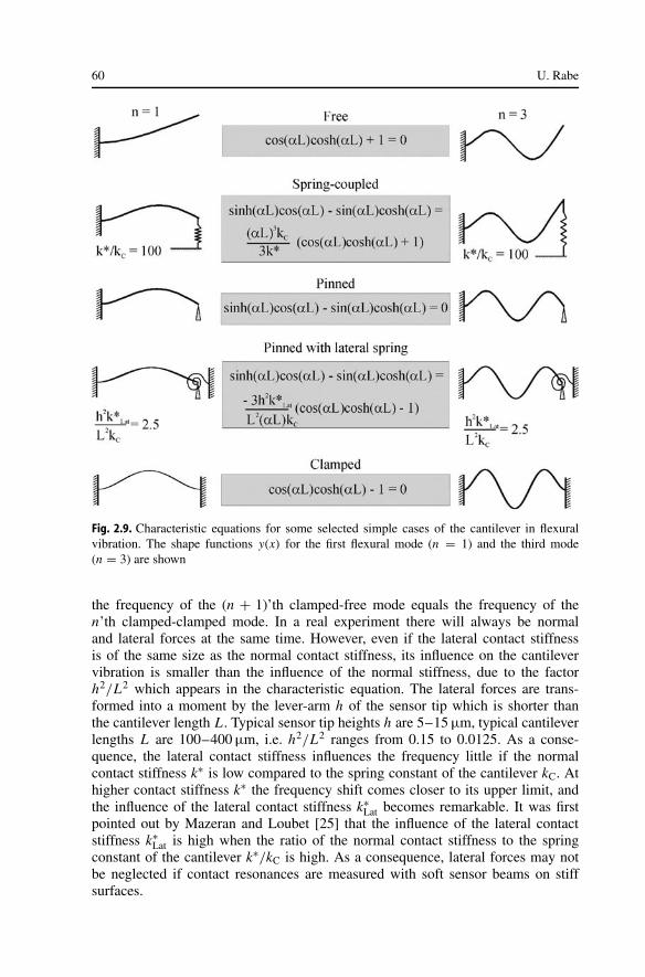
Two examples of the shape function y(x) of this case are shown in Fig. 2.9. Note that(2.42) contains the characteristic equation of the clamped-free beam and the charac-teristic equation of the clamped-pinned beam, combined by the factor (αL)3kC/3k∗.The clamped-pinned case is reached when the normal contact stiffness k∗ goes toinfinity.

Starting from the clamped-pinned case one can now add a lateral spring whichcauses feedback forces proportional to the angle of the end of the beam. A lateralspring fixed to the sensor tip is equivalent to a torsional spring which is fixed directlyto the end of the beam [25]. The characteristic equation of this case can be obtained bydividing (2.39) by U(α) and subsequently considering the case U(α) → ∞. From theremaining terms S1 + S0T(α) = 0 one obtains the following characteristic equation:

3h2k∗

Lat

L2kC(1 − cos αL cosh αL) + αL (sin αL cosh αL − sinh αL cos αL) = 0

(2.43)

Finally, when the lateral spring constant too goes to infinity, one obtains a cantileverwhich is clamped at both ends. The simplified cases of the characteristic equationdiscussed above are shown in Fig. 2.9. Furthermore, the shapes of the first (n = 1)and the third (n = 3) mode are shown. In the spring-coupled cases, the mode shapeschange continuously with the contact stiffness, Fig. 2.9 shows one example of normalcontact stiffness and one of lateral contact stiffness. Other special cases of the char-acteristic equation (2.39) were published in literature [44,60,89]. The characteristicequation for a beam with normal and lateral springs at the end at x = L was firstpublished by Wright and Nishiguchi. [89].

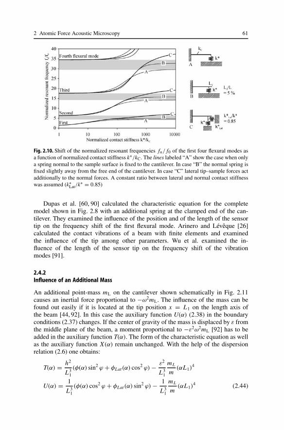
The continuous change in mode shape as a function of contact stiffness is ac-companied by a continuous change in resonant frequency. The lines labeled “A” inFig. 2.10 show the resonant frequencies of the first four flexural modes as a functionof normalized contact stiffness k∗/kC for the clamped-spring-coupled beam (2.42).In this case the contact-resonance frequencies of the n’th mode are always lowerthan the free resonant frequency of the subsequent mode (n + 1). The gaps in thespectrum between the clamped-pinned mode and the next clamped-free mode areshown as grey areas. If the sensor tip is moved away from the end of the beam(L2 > 0), the maximum possible frequency shift increases. The case of a relativetip position L2/L = 5% is shown as lines “B” in Fig. 2.10. If it happens for a modethat the distance of its last vibration node to the end of the beam becomes equalto or larger than the distance of the tip to the end, L2, this mode merges with thenext higher mode and the situation becomes difficult to survey. As the wavelengthdecreases with increasing mode number, there are always higher modes for whichthis limit is surmounted. In the experiments it is therefore better to evaluate onlymodes for which the wavelength is greater than L2.

A torsional spring at the end of the beam (lines “C” in Fig. 2.10) also in-creases the shift of the resonant frequencies to higher values, such that the gapsin the spectrum disappear. The approximations for large n in Table 2.1 show that

60 U. Rabe

Fig. 2.9. Characteristic equations for some selected simple cases of the cantilever in flexuralvibration. The shape functions y(x) for the first flexural mode (n = 1) and the third mode(n = 3) are shown

the frequency of the (n + 1)’th clamped-free mode equals the frequency of then’th clamped-clamped mode. In a real experiment there will always be normaland lateral forces at the same time. However, even if the lateral contact stiffnessis of the same size as the normal contact stiffness, its influence on the cantilevervibration is smaller than the influence of the normal stiffness, due to the factorh2/L2 which appears in the characteristic equation. The lateral forces are trans-formed into a moment by the lever-arm h of the sensor tip which is shorter thanthe cantilever length L. Typical sensor tip heights h are 5–15 µm, typical cantileverlengths L are 100–400 µm, i.e. h2/L2 ranges from 0.15 to 0.0125. As a conse-quence, the lateral contact stiffness influences the frequency little if the normalcontact stiffness k∗ is low compared to the spring constant of the cantilever kC. Athigher contact stiffness k∗ the frequency shift comes closer to its upper limit, andthe influence of the lateral contact stiffness k∗

Lat becomes remarkable. It was firstpointed out by Mazeran and Loubet [25] that the influence of the lateral contactstiffness k∗

Lat is high when the ratio of the normal contact stiffness to the springconstant of the cantilever k∗/kC is high. As a consequence, lateral forces may notbe neglected if contact resonances are measured with soft sensor beams on stiffsurfaces.

2 Atomic Force Acoustic Microscopy 61

Fig. 2.10. Shift of the normalized resonant frequencies fn/ f0 of the first four flexural modes asa function of normalized contact stiffness k∗/kC. The lines labeled “A” show the case when onlya spring normal to the sample surface is fixed to the cantilever. In case “B” the normal spring isfixed slightly away from the free end of the cantilever. In case “C” lateral tip–sample forces actadditionally to the normal forces. A constant ratio between lateral and normal contact stiffnesswas assumed (k∗

Lat/k∗ = 0.85)

Dupas et al. [60, 90] calculated the characteristic equation for the completemodel shown in Fig. 2.8 with an additional spring at the clamped end of the can-tilever. They examined the influence of the position and of the length of the sensortip on the frequency shift of the first flexural mode. Arinero and Lévêque [26]calculated the contact vibrations of a beam with finite elements and examinedthe influence of the tip among other parameters. Wu et al. examined the in-fluence of the length of the sensor tip on the frequency shift of the vibrationmodes [91].

2.4.2Influence of an Additional Mass

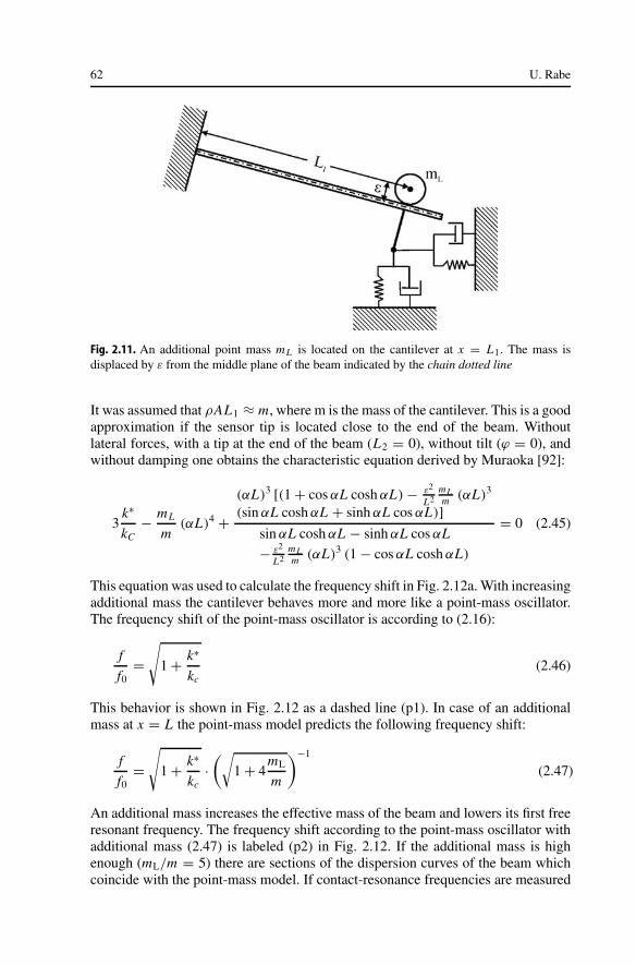
An additional point-mass mL on the cantilever shown schematically in Fig. 2.11causes an inertial force proportional to −ω2mL. The influence of the mass can befound out easily if it is located at the tip position x = L1 on the length axis ofthe beam [44, 92]. In this case the auxiliary function U(α) (2.38) in the boundaryconditions (2.37) changes. If the center of gravity of the mass is displaced by ε fromthe middle plane of the beam, a moment proportional to −ε2ω2mL [92] has to beadded in the auxiliary function T(α). The form of the characteristic equation as wellas the auxiliary function X(α) remain unchanged. With the help of the dispersionrelation (2.6) one obtains:

T(α) = h2

L31

(φ(α) sin2 ϕ + φLat(α) cos2 ϕ) − ε2

L31

mL

m(αL1)

4

U(α) = 1

L31

(φ(α) cos2 ϕ + φLat(α) sin2 ϕ) − 1

L31

mL

m(αL1)

4 (2.44)

62 U. Rabe

Fig. 2.11. An additional point mass mL is located on the cantilever at x = L1. The mass isdisplaced by ε from the middle plane of the beam indicated by the chain dotted line

It was assumed that ρAL1 ≈ m, where m is the mass of the cantilever. This is a goodapproximation if the sensor tip is located close to the end of the beam. Withoutlateral forces, with a tip at the end of the beam (L2 = 0), without tilt (ϕ = 0), andwithout damping one obtains the characteristic equation derived by Muraoka [92]:

3k∗

kC− mL

m(αL)4 +

(αL)3 [(1 + cos αL cosh αL) − ε2

L2mLm (αL)3

(sin αL cosh αL + sinh αL cos αL)]sin αL cosh αL − sinh αL cos αL

− ε2

L2mLm (αL)3 (1 − cos αL cosh αL)

= 0 (2.45)

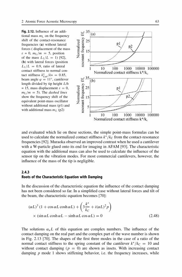
This equation was used to calculate the frequency shift in Fig. 2.12a. With increasingadditional mass the cantilever behaves more and more like a point-mass oscillator.The frequency shift of the point-mass oscillator is according to (2.16):

f

f0=√

1 + k∗

kc(2.46)

This behavior is shown in Fig. 2.12 as a dashed line (p1). In case of an additionalmass at x = L the point-mass model predicts the following frequency shift:

f

f0=√

1 + k∗

kc·(√

1 + 4mL

m

)−1

(2.47)

An additional mass increases the effective mass of the beam and lowers its first freeresonant frequency. The frequency shift according to the point-mass oscillator withadditional mass (2.47) is labeled (p2) in Fig. 2.12. If the additional mass is highenough (mL/m = 5) there are sections of the dispersion curves of the beam whichcoincide with the point-mass model. If contact-resonance frequencies are measured

2 Atomic Force Acoustic Microscopy 63

Fig. 2.12. Influence of an addi-tional mass mL on the frequencyshift of the contact-resonancefrequencies (a) without lateralforces ( displacement of the massε = 0, mL/m = 5, positionof the mass L1/L = 1) [92],(b) with lateral forces (positionL1/L = 0.9, ratio of lateralcontact stiffness to normal con-tact stiffness k∗

Lat/k∗ = 0.85,beam angle ϕ = 11, cantileverlength divided by tip height L/h= 15, mass displacement ε = 0,mL/m = 5). The dashed linesshow the frequency shift of theequivalent point-mass oscillatorwithout additional mass (p1) andwith additional mass mL (p2)

and evaluated which lie on these sections, the simple point-mass formulas can beused to calculate the normalized contact stiffness k∗/kC from the contact-resonancefrequencies [92]. Muraoka observed an improved contrast when he used a cantileverwith a W-particle glued onto its end for imaging in AFAM [93]. The characteristicequation with the additional mass can also be used to calculate the influence of thesensor tip on the vibration modes. For most commercial cantilevers, however, theinfluence of the mass of the tip is negligible.

2.4.3Roots of the Characteristic Equation with Damping

In the discussion of the characteristic equation the influence of the contact dampinghas not been considered so far. In a simplified case without lateral forces and tilt ofthe beam, the characteristic equation becomes [70]:

(αL)3 (1 + cos αL cosh αL) +(

3k∗

kC+ i(αL)2 p

)× (sin αL cosh αL − sinh αL cos αL) = 0 (2.48)

The solutions αn L of this equation are complex numbers. The influence of thecontact damping on the real part and the complex part of the wave number is shownin Fig. 2.13 [70]. The shapes of the first three modes in the case of a ratio of thenormal contact stiffness to the spring constant of the cantilever k∗/kC = 10 andwithout contact damping (p = 0) are shown as insets. With increasing contactdamping p mode 1 shows stiffening behavior, i.e. the frequency increases, while

64 U. Rabe

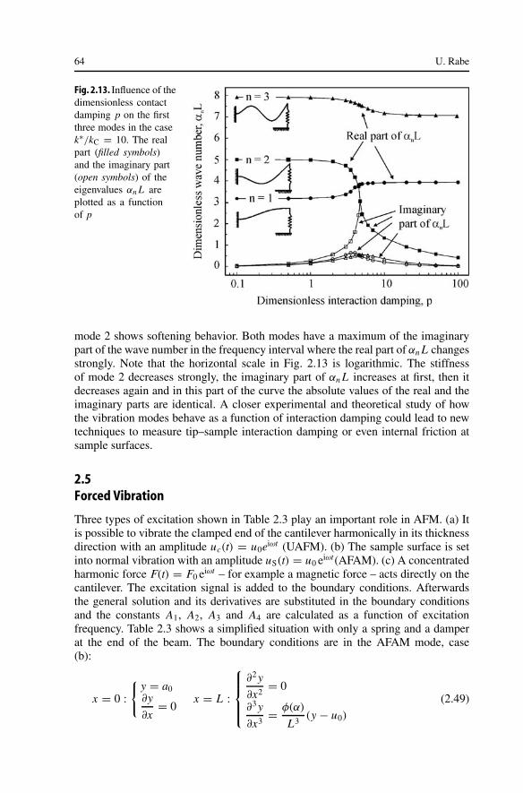
Fig. 2.13. Influence of thedimensionless contactdamping p on the firstthree modes in the casek∗/kC = 10. The realpart (filled symbols)and the imaginary part(open symbols) of theeigenvalues αn L areplotted as a functionof p

mode 2 shows softening behavior. Both modes have a maximum of the imaginarypart of the wave number in the frequency interval where the real part of αn L changesstrongly. Note that the horizontal scale in Fig. 2.13 is logarithmic. The stiffnessof mode 2 decreases strongly, the imaginary part of αn L increases at first, then itdecreases again and in this part of the curve the absolute values of the real and theimaginary parts are identical. A closer experimental and theoretical study of howthe vibration modes behave as a function of interaction damping could lead to newtechniques to measure tip–sample interaction damping or even internal friction atsample surfaces.

2.5Forced Vibration

Three types of excitation shown in Table 2.3 play an important role in AFM. (a) Itis possible to vibrate the clamped end of the cantilever harmonically in its thicknessdirection with an amplitude uc(t) = u0eiωt (UAFM). (b) The sample surface is setinto normal vibration with an amplitude uS(t) = u0 eiωt(AFAM). (c) A concentratedharmonic force F(t) = F0 eiωt – for example a magnetic force – acts directly on thecantilever. The excitation signal is added to the boundary conditions. Afterwardsthe general solution and its derivatives are substituted in the boundary conditionsand the constants A1, A2, A3 and A4 are calculated as a function of excitationfrequency. Table 2.3 shows a simplified situation with only a spring and a damperat the end of the beam. The boundary conditions are in the AFAM mode, case(b):

x = 0 :

y = a0∂y

∂x= 0

x = L :

⎧⎪⎪⎨⎪⎪⎩∂2 y

∂x2= 0

∂3 y

∂x3= φ(α)

L3(y − u0)

(2.49)

2 Atomic Force Acoustic Microscopy 65Ta

ble

2.3.

Bou

ndar

yco

nditi

ons

and

solu

tions

for

the

forc

edfle

xura

lvib

ratio

nof

aca

ntile

ver

beam

.Thr

eete

chni

ques

ofex

cita

tion

are

trea

ted:

(a)

Vib

ratio

nof

the

clam

ped

end

ofth

eca

ntile

ver,

(b)

sam

ple

surf

ace

vibr

atio

n,(c

)m

odul

ated

conc

entr

ated

forc

eac

ting

atx

=L

66 U. Rabe

From the first two boundary conditions one obtains A1 = A3 = 0, and with the thirdboundary condition the shape function becomes:

y(x) = A2(cos αx − cosh αx) + A4(sin αx − sinh αx) (2.50)

From the last boundary condition the constants A2 and A4 are calculated:

A2 = −u0φ(α)

2N(α)(sin αL + sinh αL) A4 = u0φ(α)

2N(α)(cos αL + cosh αL) (2.51)

The denominator of the two constants in the foregoing equations is the same:

N(α) = (αL)3(1 + cos αL cosh αL) + φ(α)(cosh αL sin αL − sinh αL cos αL)

(2.52)

The complex amplitude of vibration is obtained by substituting (2.51) and (2.52) in(2.50):

y(x) = u0φ(α)

2N(α)[−(sin αL + sinh αL)(cos αx − cosh αx)

+ (cos αL + cosh αL)(sin αx − sinh αx)] (2.53)

The detector, for example the laser spot of an interferometer, is usually located atthe end of the beam. In this case one only needs the amplitude at x = L, and (2.53)simplifies to:

y(L) = u0sin αL cosh αL − sinh αL cos αL

N(α)(2.54)

Commercial atomic force microscopes are generally equipped with beam-deflectionsensors. Their signal is proportional to the angle of the cantilever, given by thederivative of y(x). At the end of the beam at x = L the derivative is:

∂y

∂x

∣∣∣∣x=L

= αLu0

L

sin(αL) sinh(αL)

N(α)(2.55)

The boundary conditions and shape functions for the three mentioned cases ofexcitation are shown in Table 2.3. The amplitudes and slopes in (2.54) and in (2.55)are complex numbers. Real amplitude and phase Φ of the signals are calculated hereusing:

|y(x)| =√

Im[y(x)]2 + Re[y(x)]2 Φ(x) = − arctanIm[y(x)]Re[y(x)] (2.56)

The normalized vertical amplitude of the sensor tip dY0 and the normalized lateralamplitude dX0 of the sensor tip are defined according to:

dY0 = |y(L)| /u0 dX0 = h

∣∣∣∣∂y

∂x(L)

∣∣∣∣ /u0 (2.57)

2 Atomic Force Acoustic Microscopy 67

The lateral amplitude is the amplitude in x-direction, parallel to the length axis of thecantilever. Note that the vertical and lateral amplitudes dY0 and dX0, respectively, areonly normal and lateral to the sample surface if the cantilever is not tilted (ϕ = 0).

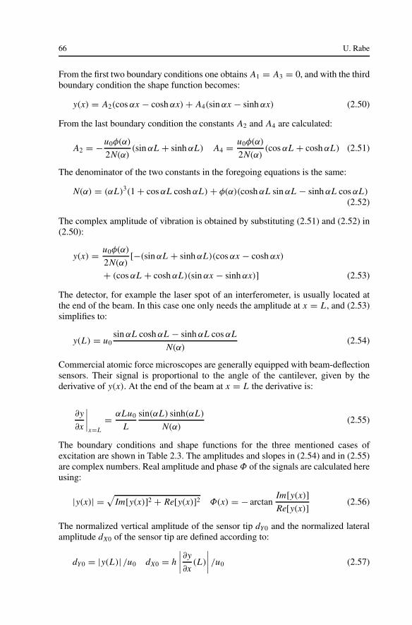
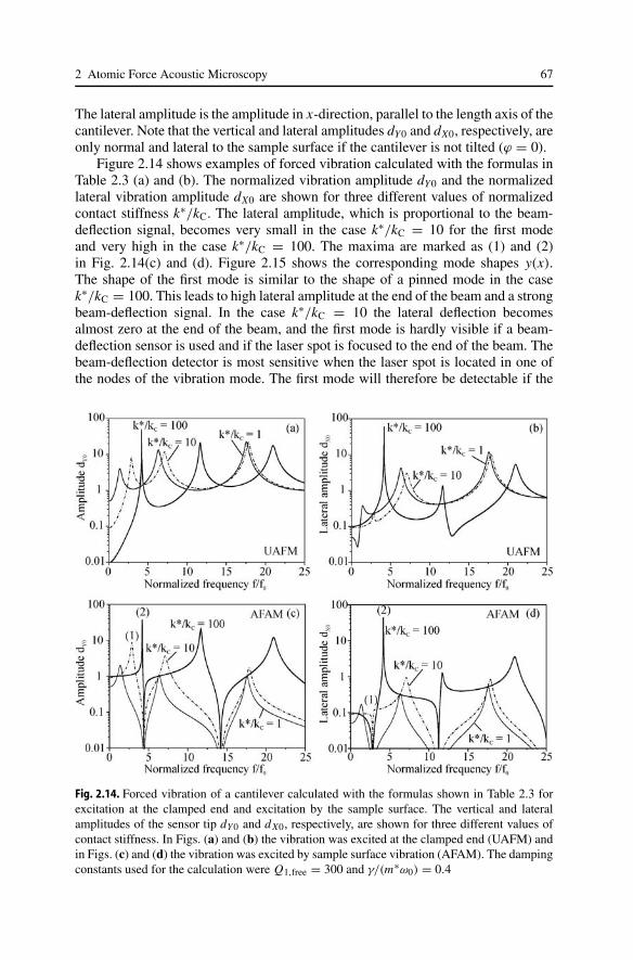
Figure 2.14 shows examples of forced vibration calculated with the formulas inTable 2.3 (a) and (b). The normalized vibration amplitude dY0 and the normalizedlateral vibration amplitude dX0 are shown for three different values of normalizedcontact stiffness k∗/kC. The lateral amplitude, which is proportional to the beam-deflection signal, becomes very small in the case k∗/kC = 10 for the first modeand very high in the case k∗/kC = 100. The maxima are marked as (1) and (2)in Fig. 2.14(c) and (d). Figure 2.15 shows the corresponding mode shapes y(x).The shape of the first mode is similar to the shape of a pinned mode in the casek∗/kC = 100. This leads to high lateral amplitude at the end of the beam and a strongbeam-deflection signal. In the case k∗/kC = 10 the lateral deflection becomesalmost zero at the end of the beam, and the first mode is hardly visible if a beam-deflection sensor is used and if the laser spot is focused to the end of the beam. Thebeam-deflection detector is most sensitive when the laser spot is located in one ofthe nodes of the vibration mode. The first mode will therefore be detectable if the

Fig. 2.14. Forced vibration of a cantilever calculated with the formulas shown in Table 2.3 forexcitation at the clamped end and excitation by the sample surface. The vertical and lateralamplitudes of the sensor tip dY0 and dX0, respectively, are shown for three different values ofcontact stiffness. In Figs. (a) and (b) the vibration was excited at the clamped end (UAFM) andin Figs. (c) and (d) the vibration was excited by sample surface vibration (AFAM). The dampingconstants used for the calculation were Q1,free = 300 and γ/(m∗ω0) = 0.4

68 U. Rabe

Fig. 2.15. Shape functions y(x) of the modes corresponding to the peaks marked as (1) and (2) inFigs. 5.1 (c) and (d). The spring and the dashpot representing the contact forces are not shownhere

laser spot is moved towards the middle of the beam. However, this decreases thesensitivity of the detection system to static forces and there is the risk that a positionmore in the middle of the beam corresponds to an antinode of one of the highermodes.

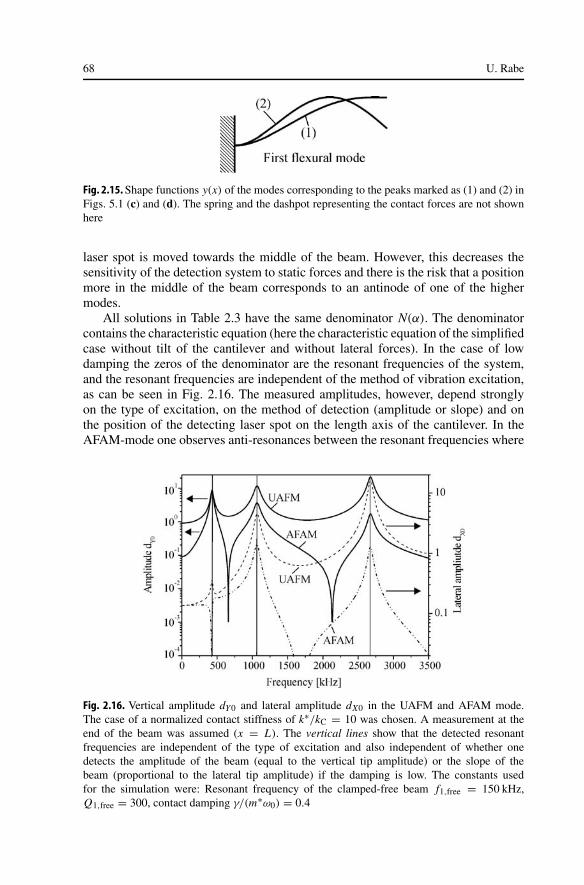
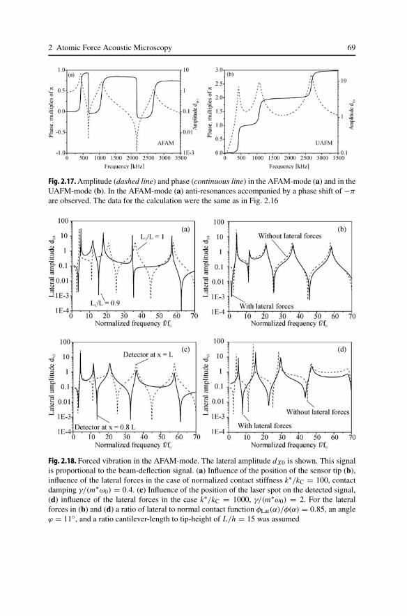
All solutions in Table 2.3 have the same denominator N(α). The denominatorcontains the characteristic equation (here the characteristic equation of the simplifiedcase without tilt of the cantilever and without lateral forces). In the case of lowdamping the zeros of the denominator are the resonant frequencies of the system,and the resonant frequencies are independent of the method of vibration excitation,as can be seen in Fig. 2.16. The measured amplitudes, however, depend stronglyon the type of excitation, on the method of detection (amplitude or slope) and onthe position of the detecting laser spot on the length axis of the cantilever. In theAFAM-mode one observes anti-resonances between the resonant frequencies where

Fig. 2.16. Vertical amplitude dY0 and lateral amplitude dX0 in the UAFM and AFAM mode.The case of a normalized contact stiffness of k∗/kC = 10 was chosen. A measurement at theend of the beam was assumed (x = L). The vertical lines show that the detected resonantfrequencies are independent of the type of excitation and also independent of whether onedetects the amplitude of the beam (equal to the vertical tip amplitude) or the slope of thebeam (proportional to the lateral tip amplitude) if the damping is low. The constants usedfor the simulation were: Resonant frequency of the clamped-free beam f1,free = 150 kHz,Q1,free = 300, contact damping γ/(m∗ω0) = 0.4

2 Atomic Force Acoustic Microscopy 69

Fig. 2.17. Amplitude (dashed line) and phase (continuous line) in the AFAM-mode (a) and in theUAFM-mode (b). In the AFAM-mode (a) anti-resonances accompanied by a phase shift of −π

are observed. The data for the calculation were the same as in Fig. 2.16

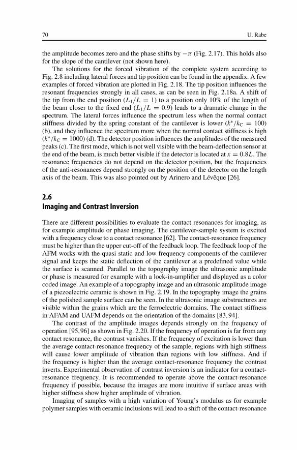
Fig. 2.18. Forced vibration in the AFAM-mode. The lateral amplitude dX0 is shown. This signalis proportional to the beam-deflection signal. (a) Influence of the position of the sensor tip (b),influence of the lateral forces in the case of normalized contact stiffness k∗/kC = 100, contactdamping γ/(m∗ω0) = 0.4. (c) Influence of the position of the laser spot on the detected signal,(d) influence of the lateral forces in the case k∗/kC = 1000, γ/(m∗ω0) = 2. For the lateralforces in (b) and (d) a ratio of lateral to normal contact function φLat(α)/φ(α) = 0.85, an angleϕ = 11, and a ratio cantilever-length to tip-height of L/h = 15 was assumed

70 U. Rabe

the amplitude becomes zero and the phase shifts by −π (Fig. 2.17). This holds alsofor the slope of the cantilever (not shown here).

The solutions for the forced vibration of the complete system according toFig. 2.8 including lateral forces and tip position can be found in the appendix. A fewexamples of forced vibration are plotted in Fig. 2.18. The tip position influences theresonant frequencies strongly in all cases, as can be seen in Fig. 2.18a. A shift ofthe tip from the end position (L1/L = 1) to a position only 10% of the length ofthe beam closer to the fixed end (L1/L = 0.9) leads to a dramatic change in thespectrum. The lateral forces influence the spectrum less when the normal contactstiffness divided by the spring constant of the cantilever is lower (k∗/kC = 100)(b), and they influence the spectrum more when the normal contact stiffness is high(k∗/kC = 1000) (d). The detector position influences the amplitudes of the measuredpeaks (c). The first mode, which is not well visible with the beam-deflection sensor atthe end of the beam, is much better visible if the detector is located at x = 0.8L. Theresonance frequencies do not depend on the detector position, but the frequenciesof the anti-resonances depend strongly on the position of the detector on the lengthaxis of the beam. This was also pointed out by Arinero and Lévêque [26].

2.6Imaging and Contrast Inversion

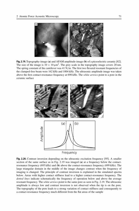
There are different possibilities to evaluate the contact resonances for imaging, asfor example amplitude or phase imaging. The cantilever-sample system is excitedwith a frequency close to a contact resonance [62]. The contact-resonance frequencymust be higher than the upper cut-off of the feedback loop. The feedback loop of theAFM works with the quasi static and low frequency components of the cantileversignal and keeps the static deflection of the cantilever at a predefined value whilethe surface is scanned. Parallel to the topography image the ultrasonic amplitudeor phase is measured for example with a lock-in-amplifier and displayed as a colorcoded image. An example of a topography image and an ultrasonic amplitude imageof a piezoelectric ceramic is shown in Fig. 2.19. In the topography image the grainsof the polished sample surface can be seen. In the ultrasonic image substructures arevisible within the grains which are the ferroelectric domains. The contact stiffnessin AFAM and UAFM depends on the orientation of the domains [83, 94].

The contrast of the amplitude images depends strongly on the frequency ofoperation [95,96] as shown in Fig. 2.20. If the frequency of operation is far from anycontact resonance, the contrast vanishes. If the frequency of excitation is lower thanthe average contact-resonance frequency of the sample, regions with high stiffnesswill cause lower amplitude of vibration than regions with low stiffness. And ifthe frequency is higher than the average contact-resonance frequency the contrastinverts. Experimental observation of contrast inversion is an indicator for a contact-resonance frequency. It is recommended to operate above the contact-resonancefrequency if possible, because the images are more intuitive if surface areas withhigher stiffness show higher amplitude of vibration.

Imaging of samples with a high variation of Young’s modulus as for examplepolymer samples with ceramic inclusions will lead to a shift of the contact-resonance

2 Atomic Force Acoustic Microscopy 71

Fig. 2.19. Topography-image (a) and AFAM amplitude-image (b) of a piezoelectric ceramic [82].The size of the image is 10 × 10 µm2. The grey scale in the topography image covers 20 nm.The spring constant of the cantilever was 41 N/m. The first two flexural resonant frequencies ofthe clamped-free beam were 162 kHz and 1004 kHz. The ultrasonic amplitude image was takenabove the first contact-resonance frequency at 698 kHz. The white arrows point to a pore in theceramic surface

Fig. 2.20. Contrast inversion depending on the ultrasonic excitation frequency [95]. A smallersection of the same surface as in Fig. 2.19 was imaged (a) at a frequency below the contact-resonance frequency (695 kHz) and (b) above the contact-resonance frequency (699 kHz). Thelarge triangular domain in the middle of the image changes contrast when the frequency ofimaging is changed. The principle of contrast inversion is explained in the simulated spectrabelow. Areas with higher contact stiffness lead to a higher contact-resonance frequency. Thedotted lines indicate schematically the frequency of operation below and above the averageresonant frequency. The white arrows point to the same pore as seen in Fig. 2.19. The ultrasonicamplitude is always low and contrast inversion is not observed when the tip is on the pore.The topography of the pore leads to a strong variation of contact stiffness and consequently toa contact-resonance frequency much different from the flat areas of the sample

72 U. Rabe

frequency within one image amounting to several multiples of the half-width of theresonant peaks. In this case it is no more possible to find a frequency which is closeto the contact-resonance maximum on both phases. Several contrast inversions mayhappen within one image and the qualitative correspondence between amplitude andstiffness is lost. Strong variations of contact stiffness are also caused by topographicalfeatures. One such example can be seen in Fig. 2.20. If the tip is above the smallpore in the ceramic which is indicated by white arrows in Fig. 2.19 and Fig. 2.20,the amplitude of vibration is low in both cases of excitation frequency. Probably,the contact-resonance frequency of this area is much different from the contact-resonance frequency of the flat surface regions.

The contrast in the amplitude images is caused by the shift of the contact-resonance frequency with contact stiffness. Furthermore, the amplitude at contactresonance varies with contact stiffness. The theoretical amplitudes at contact reso-nance of the first three modes are shown in Fig. 2.21.

Amplitude or phase imaging is a convenient method to obtain qualitative imagesof contact-stiffness variation. For quantitative evaluation, however, it is necessaryto measure the contact-resonance frequency in every pixel of the image. Kobayashi

Fig. 2.21. Vertical amplitude of the sensor tip dY0 and lateral amplitude dX0 at the contact-resonance frequency of the first three flexural modes as a function of normalized contact stiffness.A detector position at the end of the beam (x = L) was assumed and a low contact damping(γ/(m∗ω0) = 0.4) was used for the calculation. The curves were obtained by taking the amplitudemaxima of simulated contact-resonance curves. All modes have local minima in the lateralamplitude for contact stiffness values at which the slope of the shape function y(x) has localminima at x = L

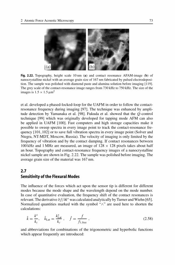
2 Atomic Force Acoustic Microscopy 73

Fig. 2.22. Topography, height scale 10 nm (a) and contact resonance AFAM-image (b) ofnanocrystalline nickel with an average grain size of 167 nm fabricated by pulsed electrodeposi-tion. The sample was polished with diamond paste and alumina solution before imaging [119].The grey scale of the contact-resonance image ranges from 730 kHz to 750 kHz. The size of theimages is 1.5 × 1.5 µm2

et al. developed a phased-locked-loop for the UAFM in order to follow the contact-resonance frequency during imaging [97]. The technique was enhanced by ampli-tude detection by Yamanaka et al. [98]. Fukuda et al. showed that the Q-controltechnique [99] which was originally developed for tapping mode AFM can alsobe applied in UAFM [100]. Fast computers and high storage capacities make itpossible to sweep spectra in every image point to track the contact-resonance fre-quency [101, 102] or to save full vibration spectra in every image point (Solver andNtegra, NT-MDT, Moscow, Russia). The velocity of imaging is only limited by thefrequency of vibration and by the contact damping. If contact resonances between100 kHz and 1 MHz are measured, an image of 128 × 128 pixels takes about halfan hour. Topography and contact-resonance frequency images of a nanocrystallinenickel sample are shown in Fig. 2.22. The sample was polished before imaging. Theaverage grain size of the material was 167 nm.

2.7Sensitivity of the Flexural Modes

The influence of the forces which act upon the sensor tip is different for differentmodes because the mode shape and the wavelength depend on the mode number.In case of quantitative evaluation, the frequency shift of the contact resonances isrelevant. The derivative ∂ f/∂k∗ was calculated analytically by Turner and Wiehn [65].Normalized quantities marked with the symbol “∧” are used here to shorten thecalculations:

k = k∗

kc, kLat = k∗

Lat

kc, f = f

f1,free, (2.58)

and abbreviations for combinations of the trigonometric and hyperbolic functionswhich appear frequently are introduced:

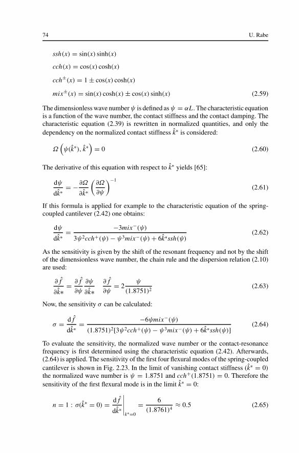
74 U. Rabe

ssh(x) = sin(x) sinh(x)

cch(x) = cos(x) cosh(x)

cch±(x) = 1 ± cos(x) cosh(x)

mix±(x) = sin(x) cosh(x) ± cos(x) sinh(x) (2.59)

The dimensionless wave number ψ is defined as ψ = αL. The characteristic equationis a function of the wave number, the contact stiffness and the contact damping. Thecharacteristic equation (2.39) is rewritten in normalized quantities, and only thedependency on the normalized contact stiffness k∗ is considered:

Ω(ψ(k∗), k∗

)= 0 (2.60)

The derivative of this equation with respect to k∗ yields [65]:

dψ

dk∗ = − ∂Ω

∂k∗

(∂Ω

∂ψ

)−1

(2.61)

If this formula is applied for example to the characteristic equation of the spring-coupled cantilever (2.42) one obtains:

dψ

dk∗ = −3mix−(ψ)

3ψ2cch+(ψ) − ψ3mix−(ψ) + 6k∗ssh(ψ)(2.62)

As the sensitivity is given by the shift of the resonant frequency and not by the shiftof the dimensionless wave number, the chain rule and the dispersion relation (2.10)are used:

∂ f

∂k∗ = ∂ f

∂ψ

∂ψ

∂k∗∂ f

∂ψ= 2

ψ

(1.8751)2(2.63)

Now, the sensitivity σ can be calculated:

σ = d f

dk∗ = −6ψmix−(ψ)

(1.8751)2[3ψ2cch+(ψ) − ψ3mix−(ψ) + 6k∗ssh(ψ)] (2.64)

To evaluate the sensitivity, the normalized wave number or the contact-resonancefrequency is first determined using the characteristic equation (2.42). Afterwards,(2.64) is applied. The sensitivity of the first four flexural modes of the spring-coupledcantilever is shown in Fig. 2.23. In the limit of vanishing contact stiffness (k∗ = 0)

the normalized wave number is ψ = 1.8751 and cch+(1.8751) = 0. Therefore thesensitivity of the first flexural mode is in the limit k∗ = 0:

n = 1 : σ(k∗ = 0) = d f

dk∗

∣∣∣∣∣k∗=0

= 6

(1.8761)4≈ 0.5 (2.65)

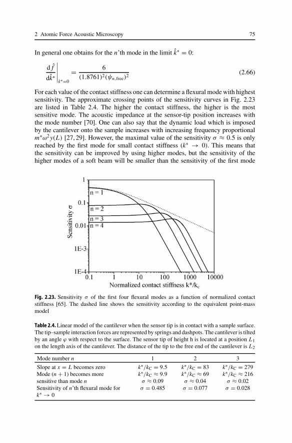
2 Atomic Force Acoustic Microscopy 75

In general one obtains for the n’th mode in the limit k∗ = 0:

d f

dk∗

∣∣∣∣∣k∗=0

= 6

(1.8761)2(ψn,free)2(2.66)

For each value of the contact stiffness one can determine a flexural mode with highestsensitivity. The approximate crossing points of the sensitivity curves in Fig. 2.23are listed in Table 2.4. The higher the contact stiffness, the higher is the mostsensitive mode. The acoustic impedance at the sensor-tip position increases withthe mode number [70]. One can also say that the dynamic load which is imposedby the cantilever onto the sample increases with increasing frequency proportionalm∗ω2 y(L) [27, 29]. However, the maximal value of the sensitivity σ ≈ 0.5 is onlyreached by the first mode for small contact stiffness (k∗ → 0). This means thatthe sensitivity can be improved by using higher modes, but the sensitivity of thehigher modes of a soft beam will be smaller than the sensitivity of the first mode

Fig. 2.23. Sensitivity σ of the first four flexural modes as a function of normalized contactstiffness [65]. The dashed line shows the sensitivity according to the equivalent point-massmodel

Table 2.4. Linear model of the cantilever when the sensor tip is in contact with a sample surface.The tip–sample interaction forces are represented by springs and dashpots. The cantilever is tiltedby an angle ϕ with respect to the surface. The sensor tip of height h is located at a position L1on the length axis of the cantilever. The distance of the tip to the free end of the cantilever is L2

Mode number n 1 2 3

Slope at x = L becomes zero k∗/kC = 9.5 k∗/kC = 83 k∗/kC = 279Mode (n + 1) becomes more k∗/kC ≈ 9.9 k∗/kC ≈ 69 k∗/kC ≈ 216sensitive than mode n σ ≈ 0.09 σ ≈ 0.04 σ ≈ 0.02Sensitivity of n’th flexural mode for σ = 0.485 σ = 0.077 σ = 0.028k∗ → 0

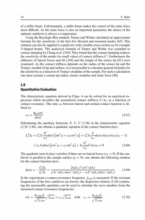
76 U. Rabe

of a stiffer beam. Unfortunately, a stiffer beam makes the control of the static forcemore difficult. As the static force is also an important parameter, the choice of theoptimal cantilever is always a compromise.

Using the Rayleigh–Ritz method, Turner and Wiehn calculated an approximateformula for the sensitivity of the first five flexural and torsional modes [65]. Thissolution can also be applied to cantilevers with variable cross-section as for exampleV-shaped beams. The analytical formula of Turner and Wiehn was extended tocontact damping by Chang et al. [103]. They found that the contact damping reducesthe sensitivity of the modes for small values of contact stiffness k∗. Furthermore theinfluence of lateral forces and tilt [104] and the length of the sensor tip [91] wereexamined. As the contact stiffness depends on the radius of the sensor tip and theYoung’s moduli of tip and surface, it is not possible to calculate general formulas forthe sensitivity as a function of Young’s modulus of the sample. For such a calculationone must assume a certain tip radius, elastic modulus and static force [96].

2.8Quantitative Evaluation

The characteristic equation derived in Chap. 4 can be solved for an analytical ex-pression which describes the normalized contact stiffness k∗/kC as a function ofcontact resonance. The ratio cP between lateral and normal contact function is de-fined as:

cP = φLat(α)

φ(α)(2.67)

Substituting the auxiliary functions X, T , U (2.38) in the characteristic equation(2.39, 2.40), one obtains a quadratic equation in the contact function φ(α):

L41S4 + L3

1S3h2

L21

φ(α)[sin2 ϕ + cP cos2 ϕ

] + L21S2

h

L1φ(α) sin ϕ cos ϕ [cP − 1]

+ L1S1φ(α)[cos2 ϕ + cP sin2 ϕ

] + S0h2

L21

φ2(α)cP = 0 (2.68)

The quadratic term in φ(α) vanishes if there are no lateral forces (cP = 0). If the can-tilever is parallel to the sample surface (ϕ = 0), one obtains the following solutionfor the contact function φ(α):

φ(α) = − L41S4

L1S1= 2(αL1)

3cch+(αL)

cch−(αL1)mix−(αL2) − cch+(αL2)mix−(αL1)(2.69)

In the experiment a contact-resonance frequency fCont is measured. If the resonantfrequencies of the free cantilever are known, the dispersion relation (2.10) contain-ing the measurable quantities can be used to calculate the wave numbers from themeasured contact-resonance frequencies:

αL = αn,freeL√fn,free

√fCont = cn

√fCont with cn := αn,freeL√

fn,free(2.70)

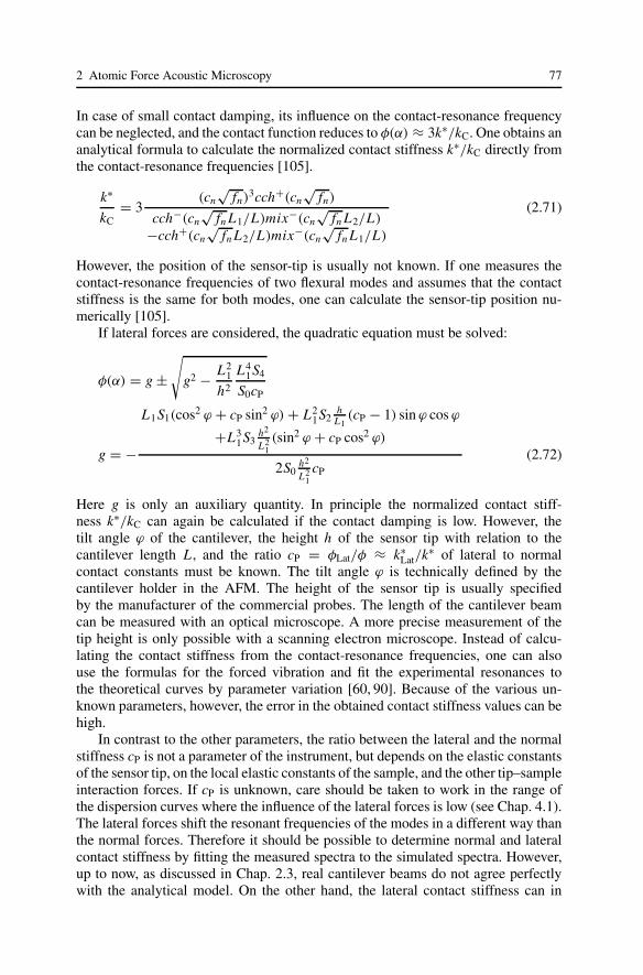
2 Atomic Force Acoustic Microscopy 77

In case of small contact damping, its influence on the contact-resonance frequencycan be neglected, and the contact function reduces to φ(α) ≈ 3k∗/kC. One obtains ananalytical formula to calculate the normalized contact stiffness k∗/kC directly fromthe contact-resonance frequencies [105].

k∗

kC= 3

(cn√

fn)3cch+(cn

√fn)

cch−(cn√

fn L1/L)mix−(cn√

fn L2/L)

−cch+(cn√

fn L2/L)mix−(cn√

fn L1/L)

(2.71)

However, the position of the sensor-tip is usually not known. If one measures thecontact-resonance frequencies of two flexural modes and assumes that the contactstiffness is the same for both modes, one can calculate the sensor-tip position nu-merically [105].

If lateral forces are considered, the quadratic equation must be solved:

φ(α) = g ±√

g2 − L21

h2

L41S4

S0cP

g = −

L1S1(cos2 ϕ + cP sin2 ϕ) + L21S2

hL1

(cP − 1) sin ϕ cos ϕ

+L31S3

h2

L21(sin2 ϕ + cP cos2 ϕ)

2S0h2

L21cP

(2.72)

Here g is only an auxiliary quantity. In principle the normalized contact stiff-ness k∗/kC can again be calculated if the contact damping is low. However, thetilt angle ϕ of the cantilever, the height h of the sensor tip with relation to thecantilever length L, and the ratio cP = φLat/φ ≈ k∗

Lat/k∗ of lateral to normalcontact constants must be known. The tilt angle ϕ is technically defined by thecantilever holder in the AFM. The height of the sensor tip is usually specifiedby the manufacturer of the commercial probes. The length of the cantilever beamcan be measured with an optical microscope. A more precise measurement of thetip height is only possible with a scanning electron microscope. Instead of calcu-lating the contact stiffness from the contact-resonance frequencies, one can alsouse the formulas for the forced vibration and fit the experimental resonances tothe theoretical curves by parameter variation [60, 90]. Because of the various un-known parameters, however, the error in the obtained contact stiffness values can behigh.

In contrast to the other parameters, the ratio between the lateral and the normalstiffness cP is not a parameter of the instrument, but depends on the elastic constantsof the sensor tip, on the local elastic constants of the sample, and the other tip–sampleinteraction forces. If cP is unknown, care should be taken to work in the range ofthe dispersion curves where the influence of the lateral forces is low (see Chap. 4.1).The lateral forces shift the resonant frequencies of the modes in a different way thanthe normal forces. Therefore it should be possible to determine normal and lateralcontact stiffness by fitting the measured spectra to the simulated spectra. However,up to now, as discussed in Chap. 2.3, real cantilever beams do not agree perfectlywith the analytical model. On the other hand, the lateral contact stiffness can in

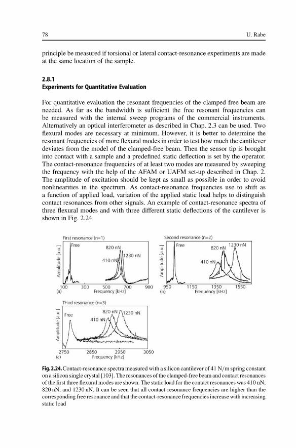
78 U. Rabe

principle be measured if torsional or lateral contact-resonance experiments are madeat the same location of the sample.

2.8.1Experiments for Quantitative Evaluation

For quantitative evaluation the resonant frequencies of the clamped-free beam areneeded. As far as the bandwidth is sufficient the free resonant frequencies canbe measured with the internal sweep programs of the commercial instruments.Alternatively an optical interferometer as described in Chap. 2.3 can be used. Twoflexural modes are necessary at minimum. However, it is better to determine theresonant frequencies of more flexural modes in order to test how much the cantileverdeviates from the model of the clamped-free beam. Then the sensor tip is broughtinto contact with a sample and a predefined static deflection is set by the operator.The contact-resonance frequencies of at least two modes are measured by sweepingthe frequency with the help of the AFAM or UAFM set-up described in Chap. 2.The amplitude of excitation should be kept as small as possible in order to avoidnonlinearities in the spectrum. As contact-resonance frequencies use to shift asa function of applied load, variation of the applied static load helps to distinguishcontact resonances from other signals. An example of contact-resonance spectra ofthree flexural modes and with three different static deflections of the cantilever isshown in Fig. 2.24.

Fig. 2.24.Contact-resonance spectra measured with a silicon cantilever of 41 N/m spring constanton a silicon single crystal [103]. The resonances of the clamped-free beam and contact resonancesof the first three flexural modes are shown. The static load for the contact resonances was 410 nN,820 nN, and 1230 nN. It can be seen that all contact-resonance frequencies are higher than thecorresponding free resonance and that the contact-resonance frequencies increase with increasingstatic load

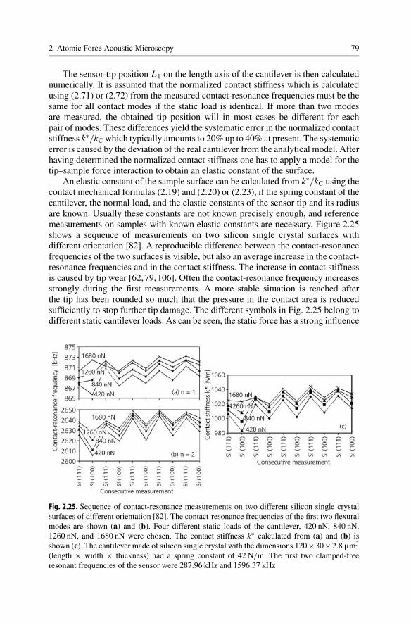
2 Atomic Force Acoustic Microscopy 79

The sensor-tip position L1 on the length axis of the cantilever is then calculatednumerically. It is assumed that the normalized contact stiffness which is calculatedusing (2.71) or (2.72) from the measured contact-resonance frequencies must be thesame for all contact modes if the static load is identical. If more than two modesare measured, the obtained tip position will in most cases be different for eachpair of modes. These differences yield the systematic error in the normalized contactstiffness k∗/kC which typically amounts to 20% up to 40% at present. The systematicerror is caused by the deviation of the real cantilever from the analytical model. Afterhaving determined the normalized contact stiffness one has to apply a model for thetip–sample force interaction to obtain an elastic constant of the surface.

An elastic constant of the sample surface can be calculated from k∗/kC using thecontact mechanical formulas (2.19) and (2.20) or (2.23), if the spring constant of thecantilever, the normal load, and the elastic constants of the sensor tip and its radiusare known. Usually these constants are not known precisely enough, and referencemeasurements on samples with known elastic constants are necessary. Figure 2.25shows a sequence of measurements on two silicon single crystal surfaces withdifferent orientation [82]. A reproducible difference between the contact-resonancefrequencies of the two surfaces is visible, but also an average increase in the contact-resonance frequencies and in the contact stiffness. The increase in contact stiffnessis caused by tip wear [62,79,106]. Often the contact-resonance frequency increasesstrongly during the first measurements. A more stable situation is reached afterthe tip has been rounded so much that the pressure in the contact area is reducedsufficiently to stop further tip damage. The different symbols in Fig. 2.25 belong todifferent static cantilever loads. As can be seen, the static force has a strong influence

Fig. 2.25. Sequence of contact-resonance measurements on two different silicon single crystalsurfaces of different orientation [82]. The contact-resonance frequencies of the first two flexuralmodes are shown (a) and (b). Four different static loads of the cantilever, 420 nN, 840 nN,1260 nN, and 1680 nN were chosen. The contact stiffness k∗ calculated from (a) and (b) isshown (c). The cantilever made of silicon single crystal with the dimensions 120×30×2.8 µm3

(length × width × thickness) had a spring constant of 42 N/m. The first two clamped-freeresonant frequencies of the sensor were 287.96 kHz and 1596.37 kHz

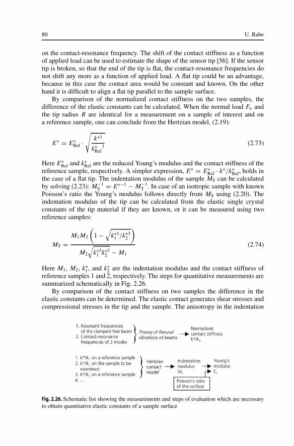
80 U. Rabe

on the contact-resonance frequency. The shift of the contact stiffness as a functionof applied load can be used to estimate the shape of the sensor tip [56]. If the sensortip is broken, so that the end of the tip is flat, the contact-resonance frequencies donot shift any more as a function of applied load. A flat tip could be an advantage,because in this case the contact area would be constant and known. On the otherhand it is difficult to align a flat tip parallel to the sample surface.

By comparison of the normalized contact stiffness on the two samples, thedifference of the elastic constants can be calculated. When the normal load Fn andthe tip radius R are identical for a measurement on a sample of interest and ona reference sample, one can conclude from the Hertzian model, (2.19):

E∗ = E∗Ref ·

√k∗3

k∗Ref

3 (2.73)

Here E∗Ref and k∗

Ref are the reduced Young’s modulus and the contact stiffness of thereference sample, respectively. A simpler expression, E∗ = E∗

Ref · k∗/k∗Ref, holds in

the case of a flat tip. The indentation modulus of the sample MS can be calculatedby solving (2.23): M−1

S = E∗−1 − M−1T . In case of an isotropic sample with known

Poisson’s ratio the Young’s modulus follows directly from MS using (2.20). Theindentation modulus of the tip can be calculated from the elastic single crystalconstants of the tip material if they are known, or it can be measured using tworeference samples:

MT =M1 M2

(1 −

√k∗3

1 /k∗32

)M2

√k∗3

1 k∗32 − M1

(2.74)

Here M1, M2, k∗1, and k∗

2 are the indentation modulus and the contact stiffness ofreference samples 1 and 2, respectively. The steps for quantitative measurements aresummarized schematically in Fig. 2.26.

By comparison of the contact stiffness on two samples the difference in theelastic constants can be determined. The elastic contact generates shear stresses andcompressional stresses in the tip and the sample. The anisotropy in the indentation

Fig. 2.26. Schematic list showing the measurements and steps of evaluation which are necessaryto obtain quantitative elastic constants of a sample surface

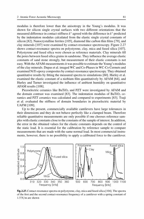
2 Atomic Force Acoustic Microscopy 81

modulus is therefore lower than the anisotropy in the Young’s modulus. It wasshown for silicon single crystal surfaces with two different orientations that themeasured difference in contact stiffness k∗ agreed with the difference in k∗ predictedby the indentation modulus calculated from the elastic single crystal constants ofsilicon [82]. Nanocrystalline ferrites [105], diamond like carbon thin films [79], andclay minerals [107] were examined by contact-resonance spectroscopy. Figure 2.27shows contact-resonance spectra on polystyrene, clay, mica and fused silica [107].Polystyrene and fused silica were chosen as reference materials. Clay minerals fillthe pores between fused silica grains in sandstone. They influence the average elasticconstants of sand stone strongly, but measurement of their elastic constants is noteasy. With the AFAM-measurements it was possible to estimate the Young’s modulusof the clay minerals. Dupas et al. imaged WC and Co-Phases in WC-Co Cermets andexamined NiTi-epoxy composites by contact-resonance spectroscopy. They obtainedquantitative results by fitting the measured spectra to simulations [60]. Hurley et al.examined the elastic constant of a niobium film quantitatively by AFAM [64], andHurley and Turner investigated the influence of ambient humidity on quantitativeAFAM results [108].

Piezoelectric ceramics like BaTiO3 and PZT were investigated by AFAM andthe domain contrast was examined [83]. The indentation modulus of BaTiO3 ce-ramics and PZT ceramics was calculated and compared to experiments [83]. Tsujiet al. evaluated the stiffness of domain boundaries in piezoelectric material byUAFM [109].

Up to the present, commercially available cantilevers have large tolerances intheir dimensions and they do not behave perfectly like a clamped beam. Thereforereliable quantitative measurements are only possible if one chooses reference sam-ples with elastic constants close to the constants of the sample of interest. In addition,the error in the obtained values for the elastic constants depends on the control ofthe static load. It is essential for the calibration by reference sample to comparemeasurements that are made with the same normal load. In most commercial instru-ments, however, there is no possibility to apply a calibrated force to the cantilever.

Fig. 2.27.Contact-resonance spectra on polystyrene, clay, mica and fused silica [104]. The spectraof the first and the second contact-resonance frequency of a cantilever with a spring constant of1.5 N/m are shown

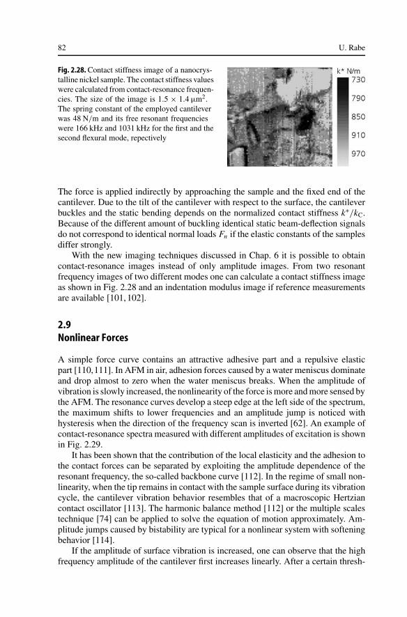
82 U. Rabe

Fig. 2.28. Contact stiffness image of a nanocrys-talline nickel sample. The contact stiffness valueswere calculated from contact-resonance frequen-cies. The size of the image is 1.5 × 1.4 µm2.The spring constant of the employed cantileverwas 48 N/m and its free resonant frequencieswere 166 kHz and 1031 kHz for the first and thesecond flexural mode, repectively

The force is applied indirectly by approaching the sample and the fixed end of thecantilever. Due to the tilt of the cantilever with respect to the surface, the cantileverbuckles and the static bending depends on the normalized contact stiffness k∗/kC.Because of the different amount of buckling identical static beam-deflection signalsdo not correspond to identical normal loads Fn if the elastic constants of the samplesdiffer strongly.

With the new imaging techniques discussed in Chap. 6 it is possible to obtaincontact-resonance images instead of only amplitude images. From two resonantfrequency images of two different modes one can calculate a contact stiffness imageas shown in Fig. 2.28 and an indentation modulus image if reference measurementsare available [101, 102].

2.9Nonlinear Forces

A simple force curve contains an attractive adhesive part and a repulsive elasticpart [110,111]. In AFM in air, adhesion forces caused by a water meniscus dominateand drop almost to zero when the water meniscus breaks. When the amplitude ofvibration is slowly increased, the nonlinearity of the force is more and more sensed bythe AFM. The resonance curves develop a steep edge at the left side of the spectrum,the maximum shifts to lower frequencies and an amplitude jump is noticed withhysteresis when the direction of the frequency scan is inverted [62]. An example ofcontact-resonance spectra measured with different amplitudes of excitation is shownin Fig. 2.29.

It has been shown that the contribution of the local elasticity and the adhesion tothe contact forces can be separated by exploiting the amplitude dependence of theresonant frequency, the so-called backbone curve [112]. In the regime of small non-linearity, when the tip remains in contact with the sample surface during its vibrationcycle, the cantilever vibration behavior resembles that of a macroscopic Hertziancontact oscillator [113]. The harmonic balance method [112] or the multiple scalestechnique [74] can be applied to solve the equation of motion approximately. Am-plitude jumps caused by bistability are typical for a nonlinear system with softeningbehavior [114].

If the amplitude of surface vibration is increased, one can observe that the highfrequency amplitude of the cantilever first increases linearly. After a certain thresh-

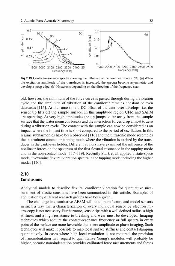
2 Atomic Force Acoustic Microscopy 83

Fig. 2.29. Contact-resonance spectra showing the influence of the nonlinear forces [62]. (a) Whenthe excitation amplitude of the transducer is increased, the spectra become asymmetric anddevelop a steep edge. (b) Hysteresis depending on the direction of the frequency scan

old, however, the minimum of the force curve is passed through during a vibrationcycle and the amplitude of vibration of the cantilever remains constant or evendecreases [115]. At the same time a DC offset of the cantilever develops, i.e. thesensor tip lifts off the sample surface. In this amplitude region UFM and SAFMare operating. At very high amplitudes the tip jumps so far away from the samplesurface that the water meniscus breaks and the interaction forces drop almost to zeroduring a vibration cycle. The contact with the sample can now be considered as animpact where the impact time is short compared to the period of oscillation. In thisregime subharmonics have been observed [116] and the ultrasonic mode resemblesthe intermittent contact or tapping mode where the vibration is excited by the trans-ducer in the cantilever holder. Different authors have examined the influence of thenonlinear forces on the spectrum of the first flexural resonance in the tapping modeand in the non-contact mode [117–119]. Recently Stark et al. applied a state-spacemodel to examine flexural vibration spectra in the tapping mode including the highermodes [120].

2.10Conclusions

Analytical models to describe flexural cantilever vibration for quantitative mea-surement of elastic constants have been summarized in this article. Examples ofapplication by different research groups have been given.

The challenge in quantitative AFAM will be to manufacture and model sensorsin such a way that a characterization of every individual sensor by electron mi-croscopy is not necessary. Furthermore, sensor tips with a well defined radius, a highstiffness and a high resistance to breaking and wear must be developed. Imagingtechniques which acquire the contact-resonance frequency or full spectra in everypoint of the surface are more favorable than mere amplitude or phase imaging. Suchtechniques will make it possible to map local surface stiffness and contact dampingquantitatively. In cases where high local resolution is not required, the precisionof nanoindentation with regard to quantitative Young’s modulus will probably behigher, because nanoindentation provides calibrated force measurements and forces

84 U. Rabe

normal to the surface. On the other hand, the development of contact mechanicsmodels for dynamic indentation is an active area of research, where nanoindentationand the AFM-techniques can stimulate each other. The potential of the high fre-quency AFM techniques like AFAM and UAFM is local resolution in the nm-rangewhich can in principle be achieved, the possibility of fast image acquisition and thepossibility to examine frequency-dependent phenomena. Furthermore, the measure-ment of frequencies is an advantage, as it avoids difficult calibration of amplitude.By combination of the results from different bending, lateral bending and torsionalmodes, elastic constants in three directions relative to the sample surface can bemeasured by AFM.

Nonlinear tip–sample forces such as friction and adhesion change the shape ofthe resonance curves in a characteristic way. Quantitative evaluation of nonlinearresonance curves is a still larger challenge than elasticity measurement. Numericalmodeling and absolute measurement of the vibration amplitudes of tip and samplewill be required in this case.

Acknowledgements. The author would like to thank W. Arnold, all colleagues, coworkers, andstudents for support and collaboration. Critical proofreading of this manuscript by S. Hirsekornis gratefully acknowledged. Part of this work was supported by the German ministry of educationand research (BMBF) in the frame of the research program “Nanoanalytik” under the contractNo. FKZ13N8326.

AAppendix

A.1Definitions

In order to calculate the forced vibration for the model shown in Fig. 2.8, includingthe angle ϕ of the cantilever, lateral forces, and tip position, abbreviations are definedfor combinations of the trigonometric and hyperbolic functions which are neededfrequently:

s±1 = sin αL1 ± sinh αL1 s±

2 = sin αL2 ± sinh αL2

c±1 = cos αL1 ± cosh αL1 c±

2 = cos αL2 ± cosh αL2

ssh1 = sin αL1 sinh αL1 ssh2 = sin αL2 sinh αL2

cch1 = cos αL1 cosh αL1 cch2 = cos αL2 cosh αL2

cch±1 = 1 ± cos αL1 cosh αL1 cch±

2 = 1 ± cos αL ′ cosh αL ′

cch+1+2 = 1 + cos α(L1 + L2) cosh α(L1 + L2)

mix±1 = sin αL1 cosh αL1 ± cos αL1 sinh hαL1

mix±2 = sin αL2 cosh αL2 ± cos αL2 sinh hαL2 (A.1)

As can be seen in Table 2.3, the formulas for the forced vibration excited by a con-centrated force acting at the free end of the beam are very similar to the solutions in

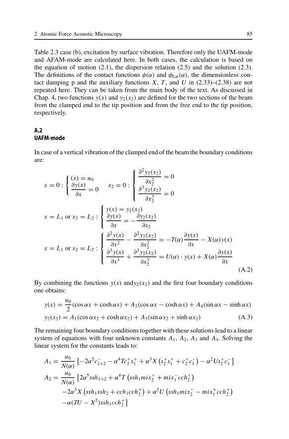
2 Atomic Force Acoustic Microscopy 85

Table 2.3 case (b), excitation by surface vibration. Therefore only the UAFM-modeand AFAM-mode are calculated here. In both cases, the calculation is based onthe equation of motion (2.1), the dispersion relation (2.5) and the solution (2.3).The definitions of the contact functions φ(α) and φLat(α), the dimensionless con-tact damping p and the auxiliary functions X, T , and U in (2.33)–(2.38) are notrepeated here. They can be taken from the main body of the text. As discussed inChap. 4, two functions y(x) and y2(x2) are defined for the two sections of the beamfrom the clamped end to the tip position and from the free end to the tip position,respectively.

A.2UAFM-mode

In case of a vertical vibration of the clamped end of the beam the boundary conditionsare:

x = 0 :

(x) = u0∂y(x)

∂x= 0

x2 = 0 :

⎧⎪⎪⎨⎪⎪⎩∂2 y2(x2)

∂x22

= 0

∂3 y2(x2)

∂x32

= 0

x = L1 or x2 = L2 :⎧⎨⎩ y(x) = y2(x2)

∂y(x)

∂x= −∂y2(x2)

∂x2

x = L1 or x2 = L2 :

⎧⎪⎪⎨⎪⎪⎩∂2 y(x)

∂x2− ∂2 y2(x2)

∂x22

= −T(α)∂y(x)

∂x− X(α)y(x)

∂3 y(x)

∂x3+ ∂3 y2(x2)

∂x32

= U(α) · y(x) + X(α)∂y(x)

∂x(A.2)

By combining the functions y(x) andy2(x2) and the first four boundary conditionsone obtains:

y(x) = u0

2(cos αx + cosh αx) + A2(cos αx − cosh αx) + A4(sin αx − sinh αx)

y2(x2) = A1(cos αx2 + cosh αx2) + A3(sin αx2 + sinh αx2) (A.3)

The remaining four boundary conditions together with these solutions lead to a linearsystem of equations with four unknown constants A1, A2, A3 and A4. Solving thelinear system for the constants leads to:

A1 = u0

N(α)

−2α5c−1+2 − α4Tc+

2 s+1 + α3 X

(s+

2 s+1 + c+

2 c−1

) − α2Us+2 c−

1

A2 = u0

N(α)

2α5ssh1+2 + α4T

(ssh1mix+

2 + mix−1 cch+

2

)−2α3 X

(ssh1ssh2 + cch1cch+

2

) + α2U(ssh1mix−

2 − mix+1 cch+

2

)−α(TU − X2)ssh1cch+

2

86 U. Rabe

A3 = u0

N(α)

−2α5c−1+2 − α4Ts−

2 s+1 + α3 X

(−c+2 s+

1 + s−2 c−

1

) + α2Uc+2 c−

1

A4 = u0

N(α)

−2α5mix+1+2 − α4T

(2ssh1cch+

2 + mix+1 mix+

2

)−2α3 X

(mix−

1 cch+2 − mix+

1 ssh2)

(A.4)

With the common denominator N(α):

N(α) = 2−2α5cch+1+2 + α4T(mix+

2 cch−1 − cch+

2 mix+1 )

− 2α3 X(cch+2 ssh1 + ssh2cch−

1 ) + α2U(mix−2 cch−

1 − cch+2 mix−

1 )

− α(TU − X2)cch+2 cch−

1 (A.5)

If the sensor tip is located at the end of the beam (L2 = 0), the constants and thedenominator simplify to:

A2 = u0

2N0(α)

−α4ssh − α3Tmix− + 2α2 Xcch + αUmix+ + (TU − X2)ssh

A4 = u0

2N0(α)α4mix+ + 2α3Tssh + 2α2 Xmix− − 2αUcch

− (TU − X2)mix+N0(α) = α4cch+ + α3Tmix+ + 2α2 Xssh

+ αUmix− + (TU − X2)cch− (A.6)

The amplitude and the slope at the end of the beam (x = L) are in this case(L2 = 0):

y(L, α) = u0

N0(α)α4c+ + α3Ts+ − α2 Xc−

∂y

∂x(L, α) = α

u0

N0(α)α4s− − α2 Xs+ + αUc− (A.7)

The forced vibration in the UAFM-mode with lateral forces and tilt of the cantilever,but without variable tip position, was discussed in a publication [121]. Unfortunately,there are several typewriting errors in the formulas in this publication. The correctboundary conditions were published for example in [104].

A.3AFAM-mode

In the case of vibration of the surface in its normal direction, one obtains componentsof excitation in vertical direction (y-direction) and in lateral direction (x-direction)in the coordinate system of the cantilever. The formulas derived here can also beused for excitation of flexural modes by lateral surface vibration. The componentsof excitation in the coordinate system of the cantilever need only to be changed inthis case. In case of normal surface vibration the boundary conditions are:

2 Atomic Force Acoustic Microscopy 87

x = 0 :

y(x) = 0∂y(x)

∂x= 0

y = L :

⎧⎪⎪⎨⎪⎪⎩∂2 y

∂x2= 0

∂3 y

∂x3= 0

x = L1 or x2 = L2 :⎧⎨⎩ y(x) = y2(x2)

∂y(x)

∂x= −∂y2(x2)

∂x2

x = L1 or x2 = L2 :

⎧⎪⎪⎨⎪⎪⎩∂2 y(x)

∂x2− ∂2 y2(x2)

∂x22

= a0 − T(α)∂y(x)

∂x− X(α)y(x)

∂3 y(x)

∂x3+ ∂3 y2(x2)

∂x32

= −b0 + U(α) · y(x) + X(α)∂y(x)

∂x(A.8)

With the components of excitation in the coordinate system of the cantilever:

a0 = −u0h

L31

φLat(α) sin ϕ b0 = u01

L31

φ(α) cos ϕ (A.9)

Using the first four boundary conditions one obtains the following solutions for thetwo sections of the cantilever:

y(x) = A2(cos αx − cosh αx) + A4(sin αx − sinh αx)

y2(x2) = A1(cos αx2 + cosh αx2) + A3(sin αx2 + sinh αx2) (A.10)

The constants are again calculated using the four boundary conditions at the tipposition and solving the linear system of equations for the constants A1, A2, A3, andA4:

A1 = −α3a0[c+

2 ssh1 + s+2 mix+

1 + c−2 cch−

1

] − α2b0[c+

2 mix−1 + s+

2 ssh1

−s−2 cch−

1

] + α (Xa0 − Tb0) c+2 cch−

1 + (Xb0 − Ua0) s+2 cch−

1

/N(α)

A2 = −α3a0[mix+

2 s−1 + ssh2c−

1 − cch+2 c+

1

] + α2b0[mix−

2 c−1 + ssh2s−

1

+cch+2 s+

1

] + α (Xa0 − Tb0) cch+2 c−

1 − (Xb0 − Ua0) cch+2 s−

1

/N(α)

A3 = α3a0

[c+

2 mix+1 − s−

2 ssh1 − s−2 cch−

1

] − α2b0[−c+

2 ssh1 + s−2 mix−

1

+c−2 cch−

1

] + α (Xa0 − Tb0) s−2 cch−

1 − (Xb0 − Ua0) c+2 cch−

1

/N(α)

A4 = α3a0

[−ssh2s+1 + mix+

2 c−1 − cch+

2 s−1

]+α2b0

[−ssh2c−1 + mix−

2 s+1 − cch+

2 c+1

]+α (Xa0 − Tb0) cch+

2 s+1 + (Xb0 − Ua0) cch+

2 c−1

/N(α) (A.11)

The denominator N(α) is the same as in the UAFM-mode (A.5). If the positiondetector is located at the end of the beam (x2 = 0), the solution simplifies to:

y2(0) = 2A1∂y2

∂x2(0) = −2αA3 (A.12)

88 U. Rabe

References

1. Hurley DC, Tewary VK, and Richards AJ (2001) Meas Sci Technol 12:14862. Every AG (2002) Meas Sci Technol 13:R213. Zieniuk JK and Latuszek A (1989) in: Shimizu H, Chubachi N, Kushibiki J (eds) Acoust

Img 17. Plenum Press, New York, p 2194. Khuri-Yakub BT, Cinbis C, Chou CH, Reinholdtsen PA (1989) in: McAvoy BR (ed) Proc.

IEEE Ultrasonics Symp, p 8055. Kulik A, Attal J, Gremaud G (1993) in: Wei Y and Gu B (eds) Acoustical Imaging 20.

Plenum Press, New York, p 2416. Quate CF, Khuri-Yakub BT, Akamine S, Hadimioglu BB (1994) United States Patent

5,319,9777. Günther P, Fischer UCh, Dransfeld K (1998) Appl Phys B 48:898. Giessibl FJ (1998) Appl Phys Lett 73:39569. Binnig G, Quate CF, Gerber Ch (1986) Phys Rev Lett 56:930

10. Kolosov O and Yamanaka K (1993) Jpn J Appl Phys 32:2211. Chilla E, Hesjedahl T, Fröhlich H-J (1997) Phys Rev B 55:1585212. Rabe U and Arnold W (1994) Appl Phys Lett 64:149313. Yamanaka K and Nakano S (1996) Jpn J Appl Phys 35:378714. Rohrbeck W and Chilla E (1992) Phys stat sol (a) 131:6915. Hesjedahl T and Behme G (2001) Europhys Lett 54:15416. Yamanaka K, Ogiso H, Kolosov O (1994) Jpn J Appl Phys 33:319717. Kolosov OV, Castell MR, Marsh CD, Briggs GAD, Kamins TI, Williams RS (1998) Phys

Rev Lett 81:104618. Yamanaka K (1996) Thin Solid Films 273:11619. Inagaki K, Kolosov OV, Briggs GAD, Wright OB (2000) Appl Phys Lett 76:183620. Inagaki K, Matsuda O, Wright OB (2002) Appl Phys Lett 80:238621. Huey BD (2002) in: Maev RG (ed) Acoust Img 26. Kluver Academic/Plenum Publishers,

p 18322. Dinelli F, Castell MR, Ritchie DA, Mason NJ, Briggs GAD, Kolosov OV (2000) Phil Mag

A 80:229923. Maivald P, Butt H-J, Gould SAC, Prater CB, Drake B, Gurley JA, Elings VB, Hansma PK

(1991) Nanotechnology 2:10324. Florin E-L, Radmacher M, Fleck B, Gaub HE (1994) Rev Sci Instr 65:63925. Mazeran P-E and Loubet J-L (1997) Tribol Lett 3:12526. Arinero R and Lévêque G (2003) Rev Sci Instr 74:10427. Troyon M, Wang Z, Pastre D, Lei HN, Hazotte A (1997) Nanotechnology 8:16328. Rosa A, Weilandt E, Hild S, Marti O (1997) Meas Sci Technol 8:129. Burnham NA, Kulik AJ, Gremaud G, Gallo PJ, Oulevey F (1996) J Vac Sci Technol

B14:79430. Oulevey F, Gremaud G, Mari D, Kulik AJ, Burnham NA, Benoit W (2000) Scripta mater

42:3131. Elings VB and Gurley JA (1993) US Patent No. 5,266,80132. Hirsekorn S, Rabe U, Arnold W (2001) Appl Phys A 72 [Suppl.]:S8733. Cretin B and Sthal F (1993) Appl Phys Lett 62:82934. Robert L and Cretin B (1999) Surf Interface Anal 27:56835. Vairac P and Cretin B (1996) Appl Phys Lett 68:46136. Cretin B and Vairac P (1997) Appl Phys Lett 71:208237. Oliver WC and Pharr GM (1992) J Mater Res 7:156438. Lorenz D, Fränzel W, Einax M, Grau P, Berg G (2001) J Mater Res 16:177639. Seyed Asif SA, Wahl KJ, Colton RJ, Warren OL (2001) J Appl Phys 90:119240. Bushan B and Li X (2003) Int Mater Rev 48:125

2 Atomic Force Acoustic Microscopy 89

41. Butt H-J and Jaschke M (1995) Nanotechnology 6:142. Salapaka MV, Bergh HS, Lai J, Majumdar A, McFarland E (1997) J Appl Phys 81:248043. Rabe U, Janser K, Arnold W (1996) in: Tortoli P and Masotti L (eds) Acoustical Imaging

22. Plenum Press, New York, p 66944. Rabe U, Janser K, Arnold W (1996) Rev Sci Instr 67:328145. Meyer G and Amer NM (1990) Appl Phys Lett 57:208946. Marti O, Colchero J, Mlynek J (1990) Nanotechnology 1:14147. Kawagishi T, Kato A, Hoshi Y, Kawakatsu H (2002) Ultramicroscopy 91:3748. Pfeiffer O, Bennewitz R, Baratoff A, Meyer E (2002) Phys Rev B 65:16140349. Reinstädtler M, Rabe U, Scherer V, Hartmann U, Goldade A, Bushan B, Arnold W (2003)

Appl Phys Lett 82:260450. Krotil HU, Weilandt E, Stifter Th, Marti O, Hild S (1999) Surf Interface Anal 27:34151. Caron A, Rabe U, Reinstädtler M, Turner JA, Arnold W (2004) Appl Phys Lett 85:639852. Drobeck T, Stark RW, Gräber M, Heckl WM (1999) New J Phys 1:15.153. Drobeck T, Stark RW, Heckl W (2001) Phys Rev B 64:04540154. Yamanaka K and Nakano S (1998) Appl Phys A 66:S31355. Yamanaka K, Noguchi A, Tsuji T, Koike T, Goto T (1999) Surf Interface Anal 27:60056. Yamanaka K, Tsuji T, Noguchi A, Koike T, Mihara T (2000) Rev Sci Instr 71:240357. Crozier KB, Yaralioglu GG, Degertekin FL, Adams JD, Minne SC, Quate CF (2000) Appl

Phys Lett 76:195058. Yaralioglu GG, Degertekin FL, Crozier KB, Quate CF (2000) J Appl Phys 87:749159. Crozier KB, Yaralioglu GG, Degertekin FL, Adams JD, Minne SC, Quate CF (2000) Proc

SPIE 4099:4860. Dupas E, Gremaud G, Kulik A, Loubet J-L (2001) Rev Sci Instr 72:389161. Rabe U and Arnold W (1994) Ann Phys 3:58962. Rabe U, Kester E, Arnold W (1999) Surf Interface Anal 27:38663. Stark RW, Drobeck T, Heckl WM (2001) Ultramicroscopy 86:20764. Hurley DC, Shen K, Jennett NM, Turner JA (2003) J Appl Phys 94:234765. Turner JA and Wiehn JS (2001) Nanotechnology 12:32266. Weaver W, Timoshenko SP, Young DH (1990) Vibration Problems in Engineering. John

Wiley, New York67. Stokey FW (1976) Vibration of Systems Having Distributed Mass and Elasticity. In: Harris

CM, Crede CE (eds) Shock and Vibration Handbook, McGraw-Hill, New York, Chapter 768. Radmacher M, Tillmann RW, Gaub HE (1993) Biophys J 64:73569. Burnham NA, Gremaud G, Kulik AJ, Gallo P-J, Oulevey F (1996) J Vac Sci Technol B

14:130870. Turner JA, Hirsekorn S, Rabe U, Arnold W (1997) J Appl Phys 82:96671. Reinstädtler M, Rabe U, Scherer V, Turner JA, Arnold W (2003) Surf Sci 532-535:115272. Hoummady M, Farnault E, Yahiro T, Kawakatsu H (1997) J Vac Sci Technol B 15:153973. Monchalin J-P (1986) IEEE Transactions UFFC-33:48574. Turner JA and Hurley DC (2003) Instrumentation, Mesure, Métrologie 3:11775. Reinstädtler M (2004) Elastische und tribologische Oberflächencharakterisierung auf

der Nanoskala mittels Torsions- und Lateralmoden von Sensorbalken der Rasterkraft-mikroskopie. PhD Thesis, Naturwissenschaftlich-Technische Fakultät III der Universitätdes Saarlandes, unpublished

76. Pietrement O and Troyon M (2000) J Colloid and Interface Science 226:16677. Schwarz UD (2003) J Colloid and Interface Science 261:9978. Johnson KL (1985) Contact mechanics. Cambridge University Press, Cambridge79. Amelio S, Goldade AV, Rabe U, Scherer V, Bushan B, Arnold W (2001) Thin solid films

392:7580. Pharr GM, Oliver WC, Brotzen F (1992) J Mat Res 7:613

90 U. Rabe

81. Vlassak JJ and Nix WD (1993) Phil Mag A67:104582. Rabe U, Amelio S, Kopycinska M, Hirsekorn S, Kempf M, Göken M, Arnold W (2002)

Surf Interface Anal 33:6583. Rabe U, Kopycinska M, Hirsekorn S, Muñoz Saldaña J, Schneider GA, Arnold W (2002)

J Phys D: Appl Phys 35:262184. Sarioglu AF, Atalar A, Degertekin FL (2004) Appl Phys Lett 84:536885. Tsuji T and Yamanaka K (2001) Nanotechnology 12:30186. Tsuji T, Irihama H, Yamanaka K (2002) JSME Int JA 45:56187. Tsuji T, Irihama H, Yamanaka K (2002) Jpn J Appl Phys 41:83288. Yamanaka K, Tsuji T, Irihama H, Mihara T (2003) Proc SPIE 5045:10489. Wright OB and Nishiguchi N (1997) Appl Phys Lett 71:62690. Dupas E (2000) Cartographie et spectroscopie des propriétés méchaniques à l’échelle du

nanomètre par spectrométrie acoustique locale à fréquence variable: Thèse no 2278, EPFLLausanne, unpublished

91. Wu T-S, Chang W-J, Hsu J-Ch (2004) Microelectronic Engineering 71:1592. Muraoka M (2002) JSME Int J A 45:56793. Muraoka M (2005) Nanotechnology 16:54294. Karapetian E, Kachanov M, Kalinin SV (2005) Phil Mag 85:101795. Rabe U, Amelio S, Hirsekorn S, Arnold W (2000) in: Halliwell M and Wells NT (eds)

Acoust Img 25. Kluwer Academic/Plenum, New York, p 25396. Rabe U, Amelio S, Kester E, Scherer V, Hirsekorn S, Arnold W (2000) Ultrasonics 38:43097. Kobayashi K, Yamada H, Matsushige K (2002) Surf Interface Anal 33:8998. Yamanaka K, Maruyama Y, Tsuji T, Nakamoto K (2001) Appl Phys Lett 78:193999. Anczykowski B, Cleveland JP, Krüger D, Elings V, Fuchs H (1998) Appl Phys A 66:S885

100. Fukuda K, Irihama H, Tsuji T, Nakamoto K, Yamanaka K (2003) Surf Sci 532-535:1145101. Hurley DC, Kos AB, Rice P (2005) Mater Res Soc Proc 838E:08.2.1102. Hurley DC, Kopycinska-Müller M, Kos AB, Geiss RH (2005) Adv Eng Mat 7:713103. Chang W-J, Fang T-H, Chou H-M (2003) Phys Lett A 312:158104. Chang W-J (2002) Nanotechnology 13:510105. Kester E, Rabe U, Presmanes L, Tailhades Ph, Arnold W (2000) J Phys Chem Solids

61:1275106. Kopycinska-Müller M, Geiss RH, Rice P, Hurley DC (2005) Mater Res Soc Proc

838E:010.16.1107. Prasad M, Kopycinska M, Rabe U, Arnold W (2002) Geophys Research Lett 29:13-1108. Hurley DC and Turner J (2004) J Appl Phys 95:2403109. Tsuji T, Ogiso H, Akedo J, Saito S, Fukuda K, Yamanaka K (2004) Jpn J Appl Phys

43:2907110. Hirsekorn S, Rabe U, Arnold W (1996) Europhysics News 27:93111. Hirsekorn S, Rabe U, Arnold W (1997) Nanotechnology 8:57112. Muraoka M and Arnold W (2001) JSME Int J A 44:396113. Turner JA (2004) J Sound and Vibration 275:177114. Nayfeh AN and Mook DT (1979) Nonlinear Oscillations. Wiley, New York115. Hirsekorn S, Rabe U, Arnold W (1997) Nanotechnology 8:57116. Burnham NA, Kulik AJ, Gremaud G (1995) Phys Rev Lett 74:5092117. Wang L (1998) Appl Phys Lett 73:3781118. Sasaki N and Tsukuda M (1999) Appl Surf Sci 140:339119. Lee SI, Howell SW, Raman A, Reifenberger R (2002) Phys Rev B 66:115409120. Stark RW, Schitter G, Stark M, Guckenberger R, Stemmer A (2004) Phys Rev B 69:085412121. Rabe U, Turner J, Arnold W (1998) Appl Phys A 66:S277122. Kopycinska-Müller, M (2005) PhD-Thesis, Naturwissenschaftlich-Technische Fakultät III

der Universität des Saarlandes, unpublished