Zero-coupon bonds assessment using a new stochastic model

ZERO-COUPON BONDS ASSESSMENT USING A NEW STOCHASTIC MODEL

M. USABEL UCM SPAIN

In many empirical situations (e.g.:Libor), the rate of interest will remain fixed at a certain level(random instantaneous rate δ i ) for a random period of time(t i ) until a new random rate should be considered, δ i+1 , that will remain for t i+1 , waiting time untill the next change in the rate of interest. Three models were developed using the approach cited above for random rate of interest and random waiting times between changes in the rate of interest. Using easy integral transforms (Laplace and Fourier) we will be able to calcu- late the moments of the probability function of the discount factor, V(t), and even its c.d.f.. The approach will also be extended to the calculation of the expected value and variance of a zero coupon bond with maturity t and we will also approximate the c.d.f. .

509

Richard Kwan

8th AFIR Colloquium, 1998: 509-524

1 INTRODUCTION

The stochastic instantaneous rate of interest has been frequently modelled using an Itô's process,

where µ and s are the expected value and the variance, Z(t) is a standard Wiener process. Many models were studied using this approach as stated in Hürlimann(1993), Ang and Sherris(1997) and Parker(1997). In these models, changes in the instantaneous rate of interest are implemented continuously.

In many empirical situations (e.g.:Libor), the rate of interest will remain fixed at a certain level(random instantaneous rate d i ) for a random period of time(t i ) until a new random rate should be considered, d i +1 , that will remain t i+1 , waiting time until the next change in the rate of interest. This last fact means that a model with continuous changes in the instantaneous rate of interest may not be very appropriate.

Let us introduce the following approach. V(t), the discount factor, can be defined

(1) where – n is a random variable that represents the total number plus 1

of changes in the rate of interest within the time interval (0, t]

the sequence on random variables that models the waiting times between changes in the rate of interest and

and It is clear that:

if n = 1 then

is a sequence of random variables for the instantaneous

rates of interest. Let us remember that and

510

assume that d j Î (0, ¥) and

Let us introduce the function:

(2)

then:

if we now define:

this expression is obtained:

and dt(x) is the first derivative of Dt(x).

(3)

(4)

Three models will be presented in section 2 using the approach cited above for random rate of interest and random waiting times between changes in the rate of interest. The first two (Models I.a and I.b) for independent rates of interest in the different waiting timesand the last one for non-independent rates, more realistic in manysituations (Model II).

In section 3, using Laplace and Fourier transforms, we will find, with Theorems 2 through 6 (based in renewal integral equations), expressions for the Laplace and Fourier transforms of a very interesting kind of functions directly related with D t (x).

In section 4, a direct expression for the moments of the probability distribution of the discount factor V(t) will be found for the three models considered.

Later, in section 5, we will see how the very c.d.f of V(t) can be approximated.

Finally, in sections 6 and 7, a zero coupon bond illustrations will be given with numerical examples.

511

2 FINANCIAL MODELS

The following models for the rate of interest will be considered

2.1 Model I.a.: i.i.d. rates of interest

Let us assume that and are sequences(mutually in-

dependent) of i.i.d. random variables with common d.f. ƒ(y) and w(x) respectively, then

(5)

with d.f.

2.2 Model I.b.: i.i.d. rates of interest with initial value.

(6)

Let us consider now the case when d 1 = d * 1 is not a random variable and t 1 follows a d.f. w 1 (x) – that could be different from w(x) – and

the sequences and are formed with i.i.d. random

variables with common d.f. ƒ(y) and w(x) respectively, as it was stated in Model l.a.. The random variable could be written:

(7)

and if t 1 > t then

Theorem 1 The c.d.f. of the random variable can be expressed:

(8)

512

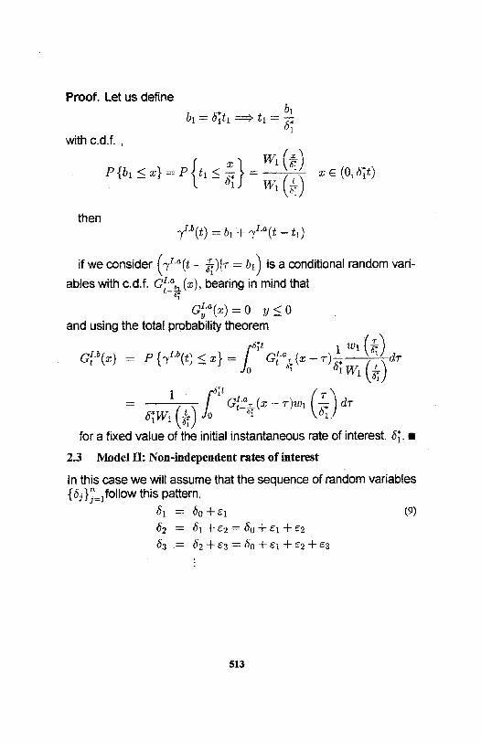
Proof. Let us define

with c.d.f. ,

then

if we consider is a conditional random vari-

ables with c.d.f. bearing in mind that

and using the total probability theorem

for a fixed value of the initial instantaneous rate of interest.

2.3 Model II: Non-independent rates of interest

In this case we will assume that the sequence of random variables follow this pattern,

(9)

513

that means that the rates of interest are non-independent random variables.

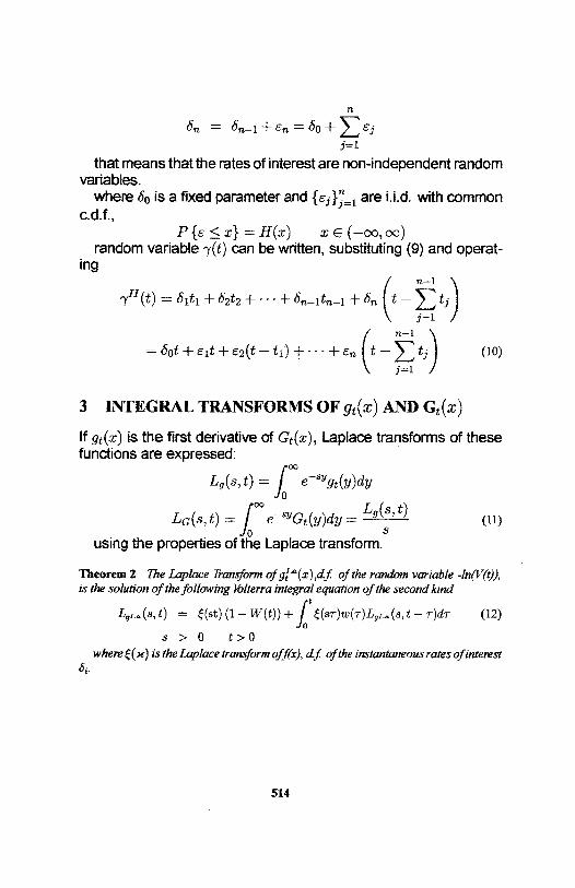
where δ 0 is a fixed parameter and are i.i.d. with common c.d.f.,

random variable can be written, substituting (9) and operat- ing

(10)

3 INTEGRAL TRANSFORMS OF gt(x) AND Gt(x)

If gt(x) is the first derivative of Gt(x), Laplace transforms of these functions are expressed:

(11)

using the properties of the Laplace transform.

Theorem 2 The Laplace Transform of of the random variable -In(V(t)), is the solution of the following Volterra integral equation of the second kind

(12)

where x (?) is the Laplace transform of f(x), d.f. of the instantaneous rates of interest d i.

514

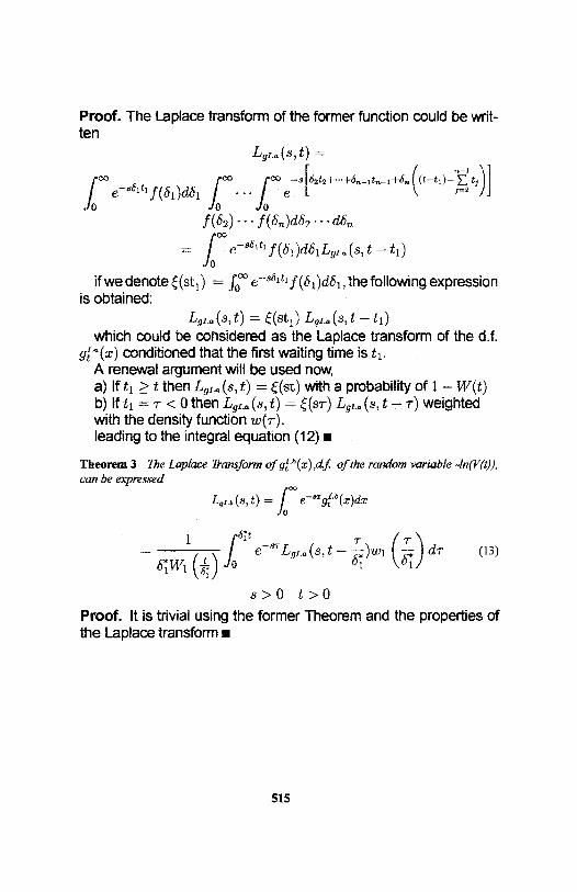
Proof. The Laplace transform of the former function could be written

if we denote the following expression is obtained:

which could be considered as the Laplace transform of the d.f. conditioned that the first waiting time is t1.

A renewal argument will be used now, a) If t 1 ≤ t then with a probability of 1 – W(t) b) If t 1 = T < 0 then weighted with the density function W(T). leading to the integral equation (12) n

Theorem 3 The Laplace Transform of of the random variable -In(V(t)), can be expressed

(13)

Proof. It is trivial using the former Theorem and the properties of the Laplace transform n

515

t of the random variable -In(V(t)), is the solution of the following Volterra integral equation of the second kind

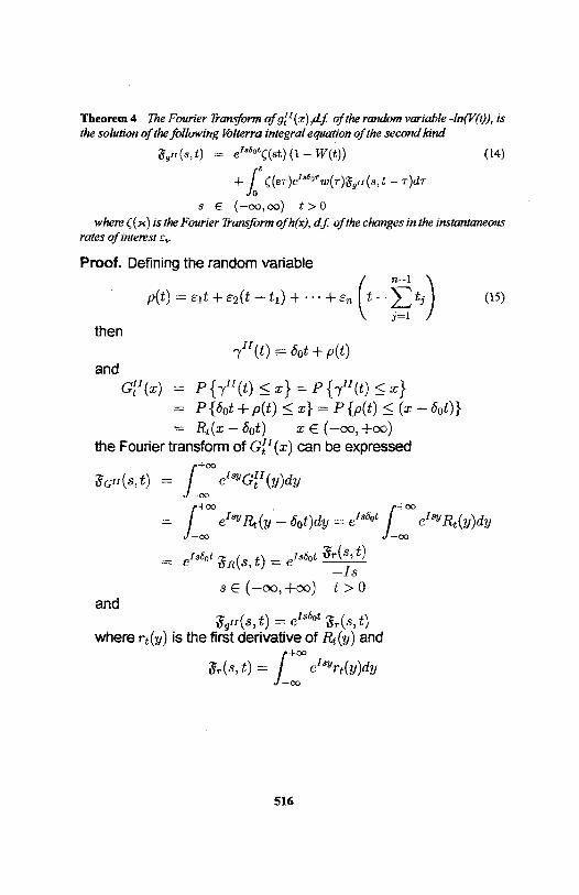
(14)

where ζ ( χ) is the Fourier Transform of h(x), d.f. of the changes in the instantaneous rates of interest ε i .

Proof. Defining the random variable

(15)

then

and

the Fourier transform of G II

t (x) can be expressed

and

where r t (y) is the first derivative of R t (y) and

516

Theorem 4 The Fourier Transform of

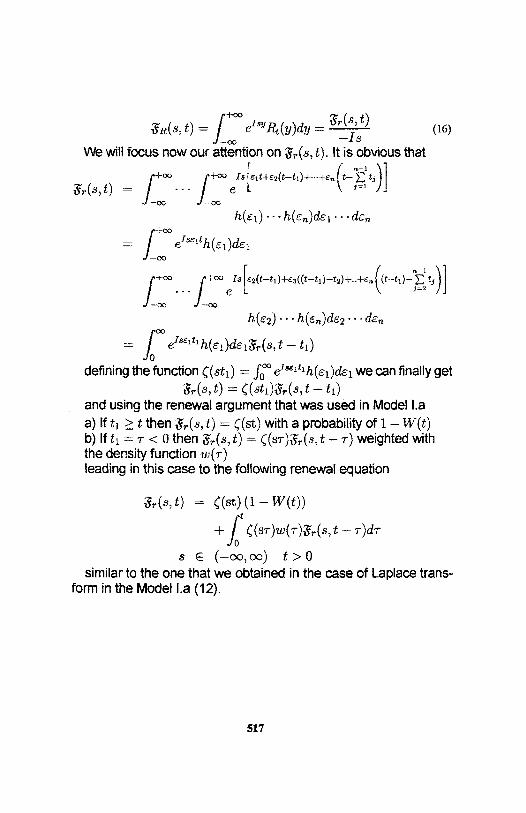
(16)

We will focus now our attention on (s, t). It is obvious that

defining the function we can finally get

and using the renewal argument that was used in Model l.a

a) If then with a probability of 1 – W(t) b) If then weighted with the density function leading in this case to the following renewal equation

similar to the one that we obtained in the case of Laplace transform in the Model l.a (12).

517

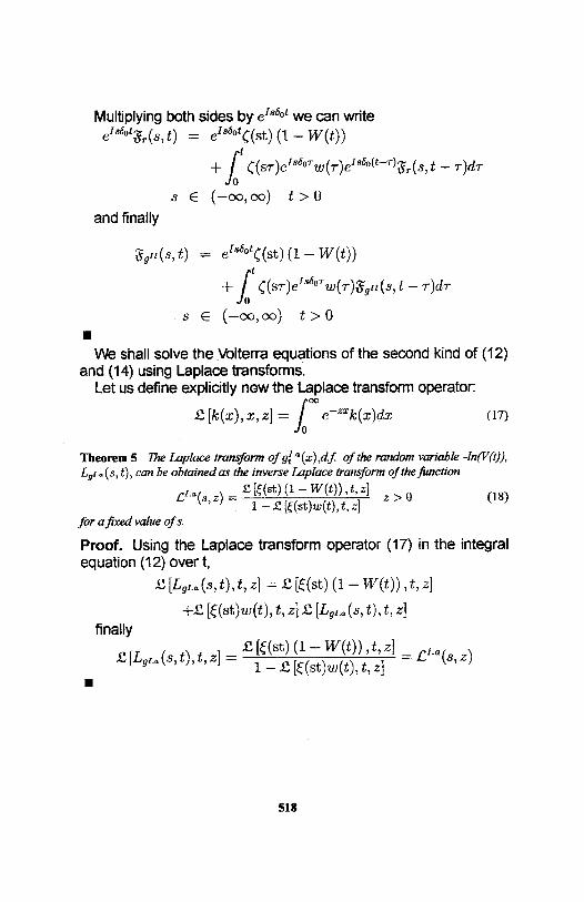
Multiplying both sides by we can write

and finally

We shall solve the Volterra equations of the second kind of (12) and (14) using Laplace transforms.

Let us define explicitly now the Laplace transform operator:

(17)

Theorem 5 The Laplace transform of of the random variable -In(V(t)), L g

I-a (s, t) , can be obtained as the inverse Laplace transform of the function

(18)

for a fixed value of s.

Proof. Using the Laplace transform operator (17) in the integral equation (12) over t,

finally

518

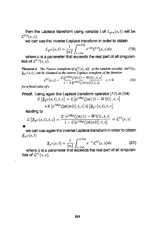
then the Laplace transform using variable t of LgI.a(s, t) will be (s, z).

we can use the inverse Laplace transform in order to obtain

(19)

where c is a parameter that exceeds the real part of all singulari- ties of (s, z).

Theorem 6 The Fourier transform of g t II (x), d.f. of the random variable -In(V(t)), (s,t), can be obtained as the inverse Laplace transform of the function

(20)

for a fixed value of s.

Proof. Using again the Laplace transform operator (17) in (14)

leading to

n

we can use again the inverse Laplace transform in order to obtain

(21)

where c is a parameter that exceeds the real part of all singulari- ties of (s, z).

519

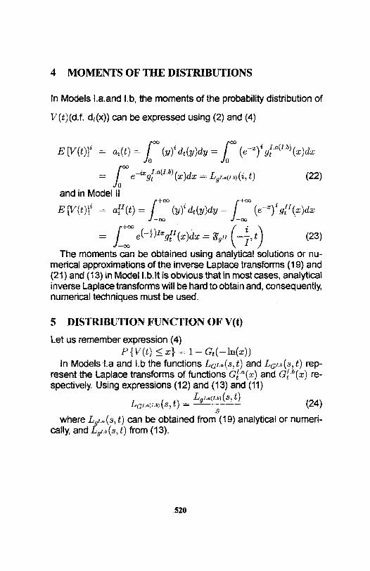
4 MOMENTS OF THE DISTRIBUTIONS

In Models I.a.and I.b, the moments of the probability distribution of

V(t)(d.f. d t (x)) can be expressed using (2) and (4)

and in Model II

(22)

(23)

The moments can be obtained using analytical solutions or numerical approximations of the inverse Laplace transforms (19) and (21) and (13) in Model I.b.It is obvious that in most cases, analytical inverse Laplace transforms will be hard to obtain and, consequently, numerical techniques must be used.

5 DISTRIBUTION FUNCTION OF V(t)

Let us remember expression (4)

In Models I.a and I.b the functions L G I.a (s, t) and L G

I.b (s, t) rep- resent the Laplace transforms of functions G t

I.a (x) and G t I.b (x) respectively. Using expressions (12) and (13) and (11)

(24)

where L g I.a (s, t) can be obtained from (19) analytical or numeri-

cally, and L g I.b (s, t) from (13).

520

Then inverting Laplace transform again could lead us to analytical

expressions or approximations of G I.a(I.b)

t (x),

(25)

where d is a number that exceeds the real part of all the singu- larities of L G I.a(I.b) (s, t).

In Model II., (s,t) stands for the Fourier transform of G II t (x). Using 16

(26)

where (s,t) can be obtained from (21) analytical or numeri- cally.

Finally, we will use the inverse Fourier transform

(27)

6 APPLICATIONS TO ASSESSMENT OF ZERO

COUPON BONDS

Let us now apply the results obtained above to a zero coupon bond of maturity t. The random variable Z represents the present value of a zero coupon bond where the actualization factor V(t) follows the considerations made in the introduction and C is the due amount (certain) at maturity time(t),

We should bear in mind that the actualization factor, V(t), is now a random variable.

It is obvious then that,

(28)

521

and the distribution function of the probability distribution of Z can be expressed,

(29)

using the results of sections 4 and 5 we will be able to obtain approximations to (28) and (29).

7 NUMERICAL ILLUSTRATION

We will now get approximations to the present value of a zero coupon bond with maturity times t=1, t=5 and t=10 and C=1 (without any loss of generality). Using (29), we will focus on the calculation of D t (x), distribution function of the discount factor V(t) (t=1, t=5 and t=10), for several values of x using model I.a. and the following assumptions;

The distributions of the waiting times will be exponential,

and λ = 1. The instantaneous rate of payments δ i will follow a Gamma dis-

tribution

y>0

with a = 1240 and b = 72, then the expected value In (1.06) and the standard deviation σ = 0.006 and

P { δ i ∈ (In(1.04), In(1.08))} 1

this last expression means that the rate of interest will fluctuate inside the interval (0.04, 0.08) with a probability very close to 1.

The values of D t (x) were obtained using the Gaver-Stehfest al- gorithm twice, first in (19) and (24) getting L G I.a (s, t) and later in (25) to obtain G I.b

t (x) and finally substituting in (4). With the assumptions made above the integrals used in the cal-

culations have an explicit formula, sea for example Gradshteyn and Ryzhik(1994). The Gaver-Stehfest method is a very efficient tool of

522

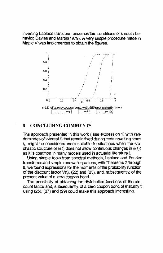
inverting Laplace transform under certain conditions of smooth be- havior, Davies and Martin (1979). A very simple procedure made in Maple V was implemented to obtain the figures.

c.d.f of a zero coupon bond with different maturity times

8 CONCLUDING COMMENTS

The approach presented in this work ( see expression 1) with random rates of interest δ i that remain fixed during certain waiting times t i, might be considered more suitable to situations when the stochastic structure of δ (t) does not allow continuous changes in δ (t)( as it is common in many models used in actuarial literature).

Using simple tools from spectral methods, Laplace and Fourier transforms and simple renewal equations, with Theorems 2 through 6, we found expressions for the moments of the probability function of the discount factor V(t), (22) and (23), and, subsequently, of the present value of a zero coupon bond.

The possibility of obtaining the distribution functions of the discount factor and, subsequently, of a zero coupon bond of maturity t using (25), (27) and (29) could make this approach interesting.

[1] Abramowitz, M. and Stegun, I.A. (1972). Handbook of Mathematical Functions. New York, N.Y. Dover Publications.

[2] Ang, A. and Sherris, M. (1997). Interest Rate Management: Developments in interest rate term structure modelling for risk management and valuation of interest-rate- dependent cash flows. North American Actuarial Journal. Volume 1, number 2. April, 1997. pgs 1-26

[3] Bowers, N.L., Gerber, H.U., Hickman, J.C. Jones, D.A. and Nesbitt, C.J. (1986) Actu- arial Mathematics. Ithasca, Ill.: Society of Actuaries.

[4] Bühlmann, H. (1995). Life insurance with stochastic interest rates. Financial Risk in Insurance. Ed. G. Ottaviani. Springer-Verlag Heidelberg

[5] Davies, B. and Martin, B. (1979). Numerical inversion of the Laplace transform: a survey and comparison of methods. Journal of computational physics 33, pgs. 1-32

[6] Gradshteyn, I. and Ryzhik, I. (1994). Table of integrals, series and products. Academic Press, Inc. San Diego, Ca.

[7] Hürlimann, W (1993). Methodes Stochastiques d’evaluation du rendiment. Proc. 3 rd

AFIR international Colloquium. Roma. [8] Parker, G. (1997). Stochastic Analysis of the interaction between investment and in-

surance risks. North American Actuarial Journal. Volume 1, number 2. April, 1997. pgs 1-26

Zero-coupon bonds assessment using a new stochastic model

Documents

Transcript of Zero-coupon bonds assessment using a new stochastic model