BANK OF GREECE

EUROSYSTEM

Economic Research Department

BANK OF GREECE

EUROSYSTEM

Special Studies Division21, E. Venizelos Avenue

Tel.:+30 210 320 3610Fax:+30 210 320 2432www.bankofgreece.gr

GR - 102 50, Athens

Special Conference Paper

ISSN: 1792-6564 FEBRUARY 2011

Special Conference Paper

The persistence of inflation in Albania

Vasilika Kota

Discussion: Sophia Lazaretou

3

BANK OF GREECE Economic Research Department – Special Studies Division 21, Ε. Venizelos Avenue GR-102 50 Athens Τel: +30210-320 3610 Fax: +30210-320 2432 www.bankofgreece.gr Printed in Athens, Greece at the Bank of Greece Printing Works. All rights reserved. Reproduction for educational and non-commercial purposes is permitted provided that the source is acknowledged. ISSN 1792-6564

Editorial

On 19-21 November 2009, the Bank of Greece co-organised with the Bank of

Albania the 3rd Annual South Eastern European Economic Research Workshop held

at its premises in Athens. The 1st and 2nd workshops were organised by the Bank of

Albania and took place in Tirana in 2007 and 2008, respectively. The main

objectives of these workshops are to further economic research in South Eastern

Europe (SEE) and extend knowledge of the country-specific features of the

economies in the region. Moreover, the workshops enhance regional cooperation

through the sharing of scientific knowledge and the provision of opportunities for

cooperative research.

The 2009 workshop placed a special emphasis on three important topics for

central banking in transition and small open SEE economies: financial and economic

stability; banking and finance; internal and external vulnerabilities. Researchers

from central banks participated, presenting and discussing their work.

The 4th Annual SEE Economic Research Workshop was organised by the Bank

of Albania and took place on 18-19 November 2010 in Tirana. An emphasis was

placed upon the lessons drawn from the global crisis and its effects on the SEE

macroeconomic and financial sectors; adjustment of internal and external

imbalances; and the new anchors for economic policy.

The papers presented, with their discussions, at the 2009 SEE Workshop are

being made available to a wider audience through the Special Conference Paper

Series of the Bank of Greece.

Here we present the paper by Vasilika Kota (Bank of Albania) and its

discussion by Sophia Lazaretou (Bank of Greece).

February, 2011

Altin Tanku (Bank of Albania) Sophia Lazaretou (Bank of Greece) (on behalf of the organisers)

THE PERSISTENCE OF INFLATION IN ALBANIA

Vasilika Kota Bank of Albania

ABSTRACT The objective of this paper is to estimate inflation persistence in Albania for the period 1993 to 2008. We apply the univariate approach with constant and time varying mean of inflation for headline and core inflation, and also test whether there are structural changes of persistence. The empirical results suggest that persistence of headline inflation was somehow higher during the inflationary periods while it started to decline after 1997, when inflationary expectations seem to have been stabilized. Therefore, monetary policy appears to be effective at reducing inflation. Empirical results for core inflation suggest that there is no structural break of persistence, which is relatively higher than persistence of headline inflation.

Keywords: inflation, persistence, Albania, univariate approach

JEL classification: E31, E37

Acknowledgements: I would like to acknowledge helpful discussions with Heather Gibson, Sophia Lazaretou and Armela Mancellari. The views expressed in this paper are those of the author and do not necessarily reflect those of the Bank of Albania and the Bank of Greece. I alone am responsible for the remaining error and omissions.

Correspondence: Vasilika Kota Research Department Sheshi Skënderbej, No. 1 Tiranë, Albania Tel: +355 4 2222 152 ext. 4080 Fax: +355 4 2223 558 E-mail: vkota@bankofalbania.org

1. Introduction

Over the past decade, inflation persistence has been widely noted and

investigated. Inflation characteristics play a central role in the design of monetary

policy and have important implications for the behaviour of private agents. Many

authors conclude that persistence is a “stylized fact”, with the Phillips Curve being

the source of this persistence. This is one key reason for using backward-looking

(persistent) elements in the Phillips Curve as a good approximation of inflation

movements.

However, no consensus has been achieved yet about the most appropriate way

to model inflation. Even if inflation persistence is observed, it is difficult to

accurately measure its degree and its continual changes. Nevertheless,

understanding the dynamics of inflation is crucial for conducting monetary policy.

The degree of inflation persistence is a key element of monetary transmission

mechanism. It is crucial for the success of monetary policy in maintaining inflation

on target. Moreover, detecting whether inflation persistence has changed over time

will greatly impact on monetary policy decisions.

Many empirical findings suggest that post war inflation exhibits high

persistence in industrial countries (see, Fryher and Moore 1995, Pivetta and Reis

2004 for the United States and O’Reilly and Whelan 2004 for the euro area etc).

However, these findings are very sensitive to the statistical techniques employed.

The inflation persistence which is observed may result due to unaccounted structural

changes, modifications of inflation targets by the central banks, different exchange

rates regimes, a price shock etc. (Levin and Piger 2003). Lack of consensus exists

also in the analysis of persistence stability. Authors such as Taylor (2000), Cogley

and Sargent (2001) and Kim, Nelson and Piger (2004) find that inflation persistence

in the US has diminished over the recent years. On the other hand, using different

econometric techniques Stock (2001) and Pivetta and Reis (2004) conclude that

inflation persistence in the US is better described as unchanged over the last

decades. The same conclusion is given by Batini (2002) and O’Relly and Whelan

(2004) for the euro area and Levin and Piger (2003) for the industrialized countries.

7

The aim of this paper is to measure, for the first time, inflation persistence in

Albania. As the Bank of Albania is preparing to launch an inflation targeting regime

in the near future, this study will be useful in determining the characteristics of

inflation. Generally, the literature suggests two distinct approaches for measuring

inflation persistence. The first method evaluates inflation persistence with simple

univariate time-series representation of inflation (univariate approach). The second

method uses structural econometric models that aim to explain inflation behaviour

with other variables besides inflation (multivariate approach). Under the univariate

approach, inflation is assumed to follow an autoregressive process and shocks are

measured in the white noise components. The multivariate approach assumes a

causal economic relationship between inflation and its determinants, and measures

persistence as the duration of the effects on inflation of the shocks to its

determinants. The basic difference between these two methods is that shocks to

inflation are not identified in the univariate approach, while the multivariate method

allows the identification of shocks hitting inflation. Therefore, the multivariate

approach provides a deeper analysis of persistence and its cause.

This paper measures inflation persistence in Albania for headline and core

inflation with the univariate approach. It also tests whether there is any structural

break during the period 1993-2008. The remainder of the paper is organized as

follows. Section 2 briefly presents inflation developments in Albania and monetary

policy changes, before proceeding to the definition of inflation persistence given in

Section 3. Section 4 presents different measures of inflation persistence based on the

univariate approach; the results obtained for each of these measures are also

presented and discussed. Section 5 tests for structural changes in inflation

persistence and presents the received evidence for different sub-periods. Finally,

Section 6 concludes.

8

2. Inflation developments: historical evidence

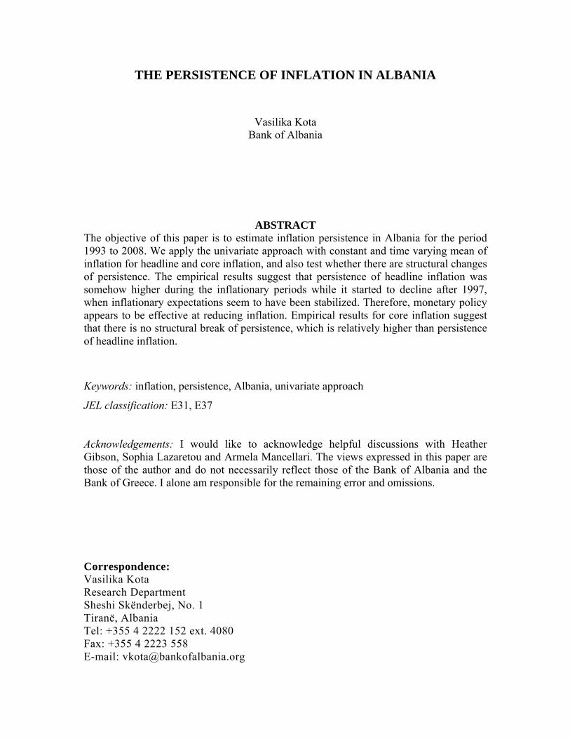
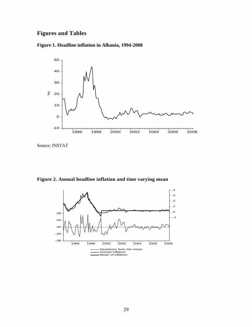
Figure 1 presents the year-on-year changes in the CPI inflation rate for Albania

starting from 1994. As the figure suggests, the country has undergone different phases of

inflation behaviour; the transition period of the 1990s is characterized by high inflation

rates which, by 1995, appeared to slow down. However, starting from 1996 there is a new

area of price increases with a strong impact following the crisis of 1997. The post-crisis

area is characterized by considerable disinflation and after 2000 inflation rates appear to

be stable to around the actual target set by the Bank of Albania, i.e. 3 1± per cent. In fact,

inflation averages 2.75 per cent, with 1.72 per cent volatility.

[Insert Figure 1 here]

During the whole sample period, monetary policy has been cautious in trying to

achieve and maintain consumer price stability. The collapse of communism in Albania at

the beginning of 1990 was followed by a year of economic collapse. Stabilization

measures introduced in 1992 had as a key objective the reduction of annual inflation.

Restriction of money growth was the main nominal anchor of the stabilization program,

supported by a careful fiscal policy aiming to eliminate monetary deficit financing and a

tight credit policy. A two-tier banking system was also introduced around this time.

Given the poor state of the domestic banking system, the adverse external debt situation

and the large budget deficit, monetary policy was based on direct instruments of money

control. At the beginning of 1996, several foreign banks began to operate in Albania, thus

creating a market for the banking system and monetary policy.

During 2000, the Bank of Albania introduced indirect instruments of monetary

policy, which included a reserve requirement, a refinancing window and a liquidity

requirement. At the same time, monetary policy also eliminated the direct control over

the interest rates.

Currently, the Bank of Albania follows a monetary target regime, with inflation

being directed through changes in the repo rate. Its main target is to achieve an annual

inflation rate of 3 1± per cent. However, in the near future, the Bank of Albania is

preparing to launch an inflation targeting regime.

9

3. Defining inflation persistence

The literature presents several definitions of inflation persistence. In their work,

Batini and Nelson (2002) distinguish three different types of persistence: a. “positive

serial correlation in inflation”; b. “lags between systematic monetary policy actions and

their (peak) effect on inflation” and c. “lagged responses of inflation to non-systematic

policy actions (i.e. policy shocks)”.

Evidence of type (a) of persistence may be found using simple estimations of

AR(1) coefficients. Following this type of definition, the high serial correlation of

inflation in post war data has been used to introduce the Philips curve for monetary

policy, thus inertia in inflation. Many studies find a decline of type (a) inflation

persistence which does not appear to be an acceptable definition of persistence. The other

definitions of inflation persistence deal with the idea of speed, i.e., the speed of the

response of inflation to a shock. If the speed is low then inflation is (highly) persistent

while if the speed is high we say that inflation is not (very) persistent.

Willis (2003) defines inflation persistence as “the speed with which inflation

returns to baseline after a shock”. What remains to be determined is the so-called baseline

or the equilibrium level of inflation. So far, when computing estimates of persistence

using the univariate approach, the empirical literature has assumed a constant long-run

equilibrium level of inflation. This assumption may or may not hold under different

circumstances. Regardless of the method used to estimate persistence, its reliability

depends on how realistic the assumed inflation equilibrium (baseline) is. As Marques

(2004) argues, there is a trade off between persistence and flexibility of inflation

equilibrium. A constant equilibrium will provide a higher estimation of inflation

persistence and vice versa. However, once we allow for flexibility of inflation

equilibrium, persistence will also change.

In our approach, inflation persistence will be defined as the speed with which

inflation returns to equilibrium after a shock. We also assume that equilibrium inflation is

exogenous and does not change due to different shocks. In the following section, various

approaches to measuring inflation persistence are introduced. We start with the

10

naïve estimates that assume a constant mean of inflation (equilibrium) and then

move on to the time varying mean approach. For each of the measures, the results of

inflation persistence estimation are presented.

4. Measuring inflation persistence

4.1 Classical analysis

The most widely used measure of persistence across the literature is the sum of

autoregressive coefficients. We start by assuming that inflation follows a stationary

autoregressive process of order p (AR(p)) which can be written as:

tjt

k

jjt επβαπ ++= −

=∑

1 (1)

where π denotes inflation at time t and tε is the residual series uncorrelated. To

measure persistence, equation (1) can be reparameterised as:

tt

k

jjtjt ερππδαπ ++∆+= −

−

=−∑ 1

1

1 (2)

where is the persistence parameter, while ∑=

=k

jj

1

βρ jδ parameters are

transformation of the AR coefficients in equation (1), kj βδ −==1 .

According to this model, inflation persistence can be defined as the speed with

which inflation converges to equilibrium after a shock in the disturbance term. In

other words, given a shock that raises inflation today by 1%, how long does it take

for the effect of the shock to die off?

Following this definition, inflation persistence is closely linked to the impulse

response function (IRF) of the AR(p) process. However, given that IRF is an

infinite-length vector, it cannot serve as a useful measure of inflation persistence.

Thus, “the sum of autoregressive coefficients” ( ) has been introduced as a ∑=

=k

jj

1

βρ

11

good indicator of persistence. Apart from this approximation, the literature suggests

several other scalar statistics to measure inflation persistence, such as “the spectrum

at zero frequency”, “the largest autoregressive root” and the “half life” (Marques

2004).

For a AR(p) process, “the spectrum at zero frequency” is given as

2

2

)1()0(

ρσε

−=h , where stands for the variance of 2

εσ tε . For a fixed , there is a

simple correspondence between this concept and

2εσ

ρ , and so they can be seen as

equivalent measures of persistence. However, the two measures can deliver different

results when testing for changes in inflation persistence over time. In the case of

“the spectrum at zero frequency”, changes may be due to or2εσ ρ , which is one of

the drawbacks of this indicator. Furthermore, ρ has an advantage over h(0) as it is

more intuitive, with a clearly defined range of potential variation (for a stationary

process it varies between -1 and 1), which is not the case for h(0) indicator.

“The largest autoregressive root” has been used in the literature as indicator of

persistence (Stock 2001). The main disadvantage of this statistic is that it is a very

poor summary measure of IRF as its shape depends also on other roots and not only

on the largest one (Andrews and Chen 2004).

Finally, the indicator of “half-life” is a useful indicator of persistence, as it

measures the number of periods during which a temporary shock displays more than half

of its initial impact to the process. In the case of an AR(1) process given by

ttt ερππ += −1 , the “half-life” indicator may be computed as HL=)ln()2/1ln(

ρ. For the

AR(p) process, the exact computation of the half-life is difficult, thus the simple

formula above is used as an approximation.

Pivetta and Reis (2004) present several drawbacks for this indicator. First, if

IRF is oscillating over time, the “half-life” estimation can understate the persistence

of the process. Second, the HL indicator does not distinguish between different IRF

speed, which may be diverse at the beginning and at the end of the shock. Third, for

highly persistent processes, the “half-life” indicator is always large but is not able to

12

indicate whether there is any change in inflation persistence over time. On the

positive side, the “half-life” outperforms the rest of the indicators as it measures

persistence in units of time. This unit is easier to be comprehended and discussed as

compared to other indicators presented above.

We should keep in mind that the above-mentioned indicators provide only an

estimation of the persistence and not the true measures of this process. This is

because they cannot fully capture the existence of different shapes in the impulse

response functions of inflation following a given shock. In general, any scalar

measure of persistence should be seen as providing only an estimate of the “average

speed” with which inflation converges to equilibrium after a shock. The more

uniform is the speed at convergence throughout the convergence period, the more

reliable is the scalar measure of persistence.

Summing up, we can conclude that two out of the four measures of persistence

discussed above, namely “the sum of autoregressive coefficients” and the “spectrum

at zero frequency”, can be referred as close substitutes for a fixed sample period.

The largest autoregressive root appears to be a poor measure of persistence, while

despite its limitations, the “half-life” indicator measures persistence in units of time,

which is useful for communication purposes.

In the following sections, we focus on ρ parameter and the “half life

indicator” to measure persistence. “The sum of the autoregressive coefficients” is

linked directly to the mean reversion coefficient of the series, while the half life

measure persistence in units of time.

4.1.1 Results for the ρ parameter

To obtain a measure of inflation persistence, we estimate the following

equation:

tt

k

jjtjt ερππδαπ +++= −

−

=−∑ 1

1

1 (3)

where tπ is annual inflation, i.e. 12−−= ttt ppπ and is the logarithm of CPI.

There are a few reasons why we study the persistence of annual inflation. First, other

tp

13

possibilities such as using month-on-month and quarter-on-quarter changes of price level

are associated with seasonality, which may contaminate the true extent of persistence.

Second, central banks set their inflation targets as year-on-year changes in the price level.

Third, there are many findings such as from Aron and Muellbauer (2006) that claim that

year-on-year inflation rates also capture the dynamics of month-on-month inflation. On

the other hand, when using annual inflation to measure persistence, it is expected to get

high autoregression coefficients due to the presence of a moving average component.

This may result in estimating higher persistence from what it is exhibited from the actual

series of inflation. Therefore, in this paper inflation is also calculated as month-on-month

inflation annualized. As inflation is calculated on a monthly basis, one has to take into

account seasonality, which we have corrected by applying the Tramo/Seats procedure.

To ensure that our results are not specific to a particular measure of inflation, we

analyse the properties of two different price indices, i.e. the consumer price index (CPI)

and core CPI. Core CPI is obtained with the method of permanent exclusion of certain

volatile CPI components as presented by Celiku and Hoxholli (2007). We focus our

analysis on the sample period from 1993 to 2008 for which headline CPI data are

available, and from 1998 to 2008 for core CPI.

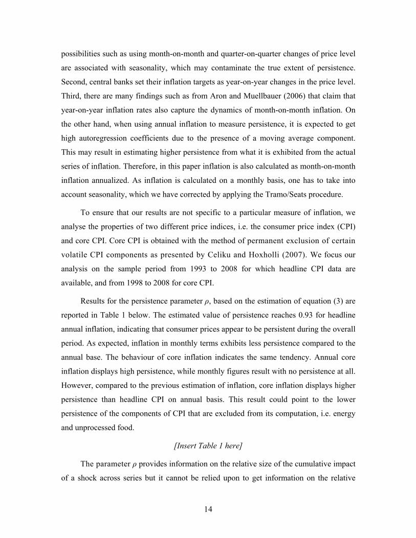
Results for the persistence parameter ρ, based on the estimation of equation (3) are

reported in Table 1 below. The estimated value of persistence reaches 0.93 for headline

annual inflation, indicating that consumer prices appear to be persistent during the overall

period. As expected, inflation in monthly terms exhibits less persistence compared to the

annual base. The behaviour of core inflation indicates the same tendency. Annual core

inflation displays high persistence, while monthly figures result with no persistence at all.

However, compared to the previous estimation of inflation, core inflation displays higher

persistence than headline CPI on annual basis. This result could point to the lower

persistence of the components of CPI that are excluded from its computation, i.e. energy

and unprocessed food.

[Insert Table 1 here]

The parameter ρ provides information on the relative size of the cumulative impact

of a shock across series but it cannot be relied upon to get information on the relative

14

timing of the absorption of a shock. To get information on the latter, we need to rely on

the HL indicator instead even though HL provides only a rough summarization of the full

timing information contained in the entire impulse response function.

4.1.2 Results for the “half-life” indicator

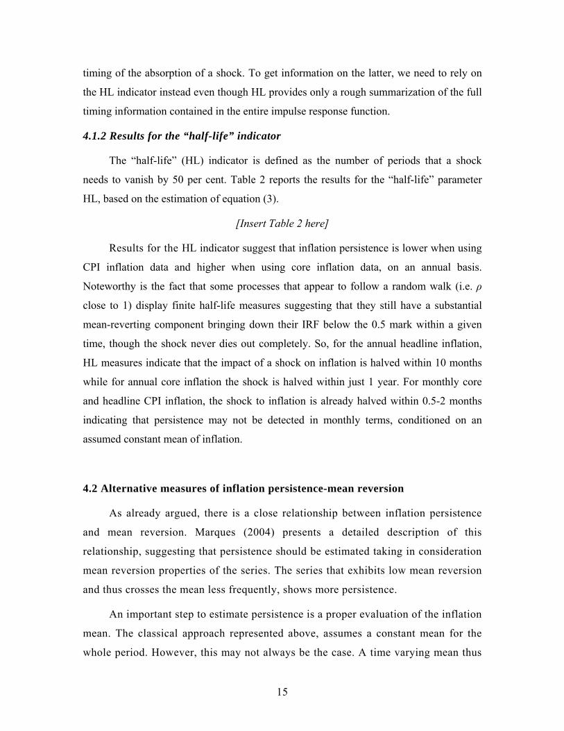
The “half-life” (HL) indicator is defined as the number of periods that a shock

needs to vanish by 50 per cent. Table 2 reports the results for the “half-life” parameter

HL, based on the estimation of equation (3).

[Insert Table 2 here]

Results for the HL indicator suggest that inflation persistence is lower when using

CPI inflation data and higher when using core inflation data, on an annual basis.

Noteworthy is the fact that some processes that appear to follow a random walk (i.e. ρ

close to 1) display finite half-life measures suggesting that they still have a substantial

mean-reverting component bringing down their IRF below the 0.5 mark within a given

time, though the shock never dies out completely. So, for the annual headline inflation,

HL measures indicate that the impact of a shock on inflation is halved within 10 months

while for annual core inflation the shock is halved within just 1 year. For monthly core

and headline CPI inflation, the shock to inflation is already halved within 0.5-2 months

indicating that persistence may not be detected in monthly terms, conditioned on an

assumed constant mean of inflation.

4.2 Alternative measures of inflation persistence-mean reversion

As already argued, there is a close relationship between inflation persistence

and mean reversion. Marques (2004) presents a detailed description of this

relationship, suggesting that persistence should be estimated taking in consideration

mean reversion properties of the series. The series that exhibits low mean reversion

and thus crosses the mean less frequently, shows more persistence.

An important step to estimate persistence is a proper evaluation of the inflation

mean. The classical approach represented above, assumes a constant mean for the

whole period. However, this may not always be the case. A time varying mean thus

15

appears to be more useful than a constant one. In order to stay within the univariate

approach, we use statistical models to extract the mean of inflation. We also check

by using the Hodrick-Prescott filter as another useful estimation of the time varying

mean of inflation.

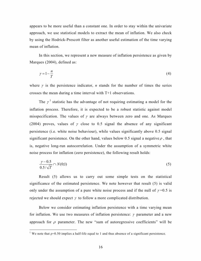
In this section, we represent a new measure of inflation persistence as given by

Marques (2004), defined as:

Tn

−=1γ (4)

where γ is the persistence indicator, n stands for the number of times the series

crosses the mean during a time interval with T+1 observations.

The γ 1 statistic has the advantage of not requiring estimating a model for the

inflation process. Therefore, it is expected to be a robust statistic against model

misspecification. The values of γ are always between zero and one. As Marques

(2004) proves, values of γ close to 0.5 signal the absence of any significant

persistence (i.e. white noise behaviour), while values significantly above 0.5 signal

significant persistence. On the other hand, values below 0.5 signal a negative ρ , that

is, negative long-run autocorrelation. Under the assumption of a symmetric white

noise process for inflation (zero persistence), the following result holds:

)1;0(/5.0

5.0 NT∩

−γ (5)

Result (5) allows us to carry out some simple tests on the statistical

significance of the estimated persistence. We note however that result (5) is valid

only under the assumption of a pure white noise process and if the null of γ =0.5 is

rejected we should expect γ to follow a more complicated distribution.

Below we consider estimating inflation persistence with a time varying mean

for inflation. We use two measures of inflation persistence: γ parameter and a new

approach for ρ parameter. The new “sum of autoregressive coefficients” will be

1 We note that ρ=0.50 implies a half-life equal to 1 and thus absence of a significant persistence.

16

determined by estimating persistence taking into account of the deviations from the

time varying mean. We start with the same autoregressive representation of

inflation, i.e.

tjt

k

jjt επβαπ ++= −

=∑

1 (6)

Equation (6) can be equivalently represented as:

( ) ( ) tjtjt

k

jjtt εµπβαµπ +−+=− −−

=∑

1 (7)

or further as:

( ) ( ) tttjtjt

k

jjtt εµπρµπδµπ +−+−∆=− −−−−

=∑ )( 11

1 (8)

which corresponds to the classical model used in section 4.1. Since we estimate the

deviations of inflation from its mean, there is no a constant term.

4.2.1 Results for the γ parameter and ρ parameter with time varying mean

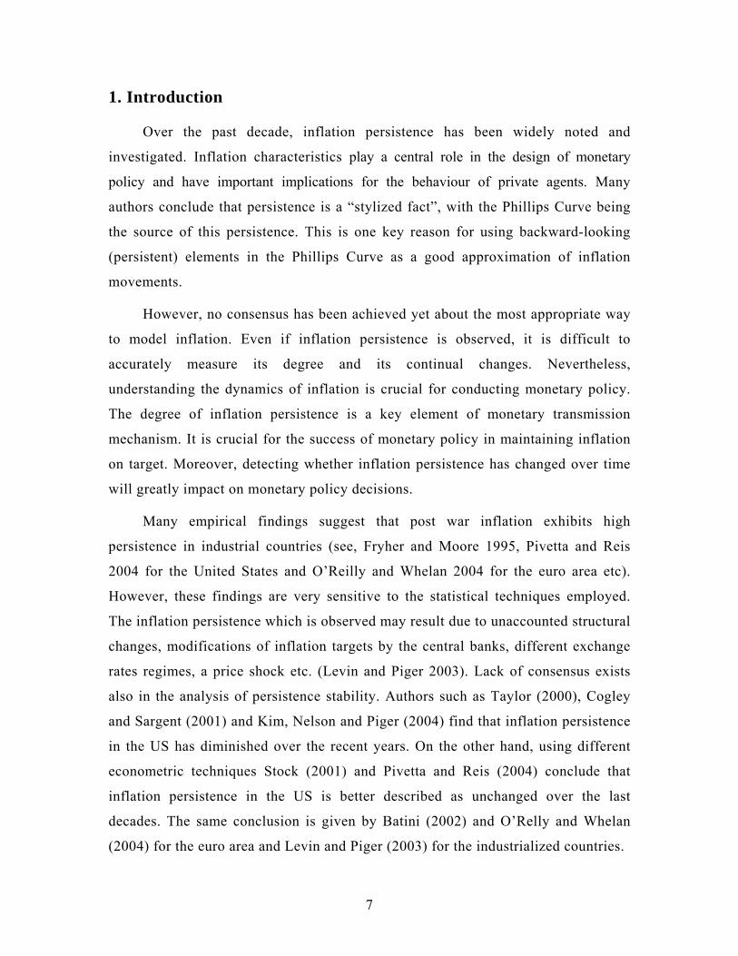
We first start by using statistical estimations to extract the time varying mean

of inflation. Figure 2 presents the developments of the annual headline inflation

rate. Simple visual inspection suggests that we can distinguish four distinct periods.

The first period stretches from the beginning of the sample until the middle of 1995

and exhibits a downward trend. During the second period, from mid 1995 to

beginning of 1997, inflation shows an upward trend. This is a clear example of why

assuming a constant mean of inflation does not appear to be a realistic approach.

The third period is composed of a downward trend that took place during 1998-

1999. Finally, during the fourth period from 2000 onwards, inflation does not seem

to exhibit a clear increasing or decreasing time trend.

The mean of annual inflation in Figure 2 is obtained as the fitted values of the

following regression model:

tπ =-0.089 + 0.03*t1 + 0.012*t2 + 0.017*t3 + 0.17*c1

p-value (0.00) (0.00) (0.00) (0.00) (0.00)

17

that is estimated for the period 1994m12 to 2008m08. The variables are defined as

follows: t1-time trend for the period 1993m12-1995m7; t2-time trend for the period

1995m8- 1998m1; t3-time trend for the period 1998m2- 1999m10 and c1-constant for the

period 1999m11-2008m8.

[Insert Figure 2 here]

Using the definition presented in section 4.2, we measure inflation persistence as

the portion of mean crossings (γ ) and test for its statistical significance. In order to

check for other behaviors of time varying mean, we also estimate inflation mean

using the Hodrick-Prescott filter. Finally, “the sum of autoregressive coefficient” is

derived from estimating equation (8). The same approach is followed for monthly

headline inflation and core inflation indicators. The estimation process of time varying

mean for these indicators is given in an annex at the end of the paper. Below we present

the results of γ parameter and ρ parameter.

[Insert Table 3 here]

All the estimates for inflation persistence using the γ parameter are

statistically significant. Mean reversion properties of headline inflation in annual

and monthly terms indicate the presence of persistence. However, ρ parameter of

annual inflation is much lower when measured with time varying mean, than with

constant mean, indicating that inflation exhibits some persistence but not as high as

suggested by the classical approach. As in the case of the classical analysis, annual

core inflation exhibits higher persistence than headline inflation. While, monthly

core inflation does not indicate persistence using the ρ parameter, the portion of

mean crossing results statistically significant. It also follows that monthly core inflation

does exhibit low persistence. It thus entails that the empirical finding concerning inflation

persistence can change noticeably as the assumption of inflation mean changes.

By putting together the results of the classical analysis and the time varying mean

estimation, we conclude that headline inflation in annual and monthly terms in Albania

exhibits persistence. Inflation persistence in annual terms is always higher than that in

18

monthly terms. Other authors (see, for example, Altissimo, Ehrmann and Smets 2006)

find similar results; the series based on quarter-on-quarter changes is found to be less

persistent compared to year-on-year changes.

Annual core inflation exhibits relatively higher persistence than headline inflation.

Other studies also find similar results. For example, Hondroyiannis and Lazaretou (2007)

show that core CPI inflation reveals a substantial rise in the serial correlation of Greek

inflation compared to headline inflation. Further, Gadzinski and Orlandi (2004) using the

data for the euro area and the US inflation rate conclude that core inflation usually

displays higher persistence than the other inflation measurements. Finally monthly core

inflation in Albania verifies the presence of some persistence when the assumption of a

constant mean is abandoned.

5. Testing for structural changes in inflation persistence

Recent literature suggests that there might be possible shifts in inflation

persistence over the sample taken in consideration. To test for a structural change in

inflation persistence in Albania, we apply the Quandt-Andrews Breakpoint test. The

Quandt-Andrews Breakpoint Test tests for one or more unknown structural breakpoints in

the sample for a specified equation. The idea behind the Quandt-Andrews test is that a

single Chow Breakpoint Test is performed at every observation between two dates, i.e. 1τ

and 2τ . The test statistics from those Chow tests are then summarized into one test

statistic for a test against the null hypothesis of no breakpoints between 1τ and 2τ . From

each individual Chow Breakpoint Test, two statistics are retained, the Likelihood Ratio

F-statistic and the Wald F-statistic. The individual test statistics can be summarized into

three different statistics: the Sup or Maximum statistic, the Exp Statistic and the Ave

statistic.

• The Maximum statistic is simply the maximum of the individual Chow F-

statistics:

21

))(max(ττττ

<<= FMaxF (9)

19

• The Exp statistic takes the form:

)))(21exp(1ln(

2

1

ττ

ττF

kExpF ∑

=

= (10)

• The Ave statistic is the simple average of the individual F-statistics:

( )∑=

=2

1

1 τ

τττF

kAveF (11)

All these test statistics are used to detect possible structural breakpoints in the

sample under study.

5.1 Structural breaks in inflation persistence with a constant mean

We start by testing for structural changes in inflation persistence for headline

CPI with a constant mean. All three summary statistic measures used reject the null

hypothesis of no structural breakpoint at the 5 % level for the annual data points.

Thus, a break point between the first and the second month of 1998 is detected.

Equation (3), therefore, is estimated over the two sub-samples: 1993m12-1998m1

and 1998m2-2008m8. When conducting the analysis on monthly inflation, the test

suggests that there is one structural break in 1997m04. The indicators of persistence

are estimated over the two sub-samples, 1993m12-1998m1 and 1998m2-2008m8.

Table 4 presents the estimates of persistence and the sample mean in the form

of a univariate representation of the annual and inflation rate for the two different

sub-periods.

[Insert Table 4 here]

As it can be seen from the table, Albania experiences a sizeable shift in the

average level of CPI inflation. The sample mean of the headline inflation rate falls

significantly between the two periods in question, both for annual and monthly

inflation. The results indicate that there is a substantial drop in the sample mean

from a yearly average level of 16 per cent to 4 per cent after 1998. Furthermore, the

variance before and after the break decreases; headline inflation is 2.1 times less volatile

20

in disinflation relative to the period of high inflation. However, the shift in persistence

is rather small, ρ decreases from 0.89 to about 0.83. The half-life indicator also

confirms that IRF is brought down below the 0.5 mark in 5-6 months for the first sub-

sample, and 4-5 months for the second one. Overall, according to the autoregressive

estimates, there appears to have been a sizeable shift in annual inflation mean in Albania

over the last 15 years, but only a small shift in inflation persistence.

The results for monthly inflation are different. It seems that there is a substantial

drop in the sample mean from an average level of 15.5 per cent to 3.9 per cent after

1997m4. However, autoregressive estimation does not indicate persistence for the first

sub-period. After 1997m4, monthly inflation exhibits somehow higher persistence

than that over the whole sample period. The variance before and after the break

decreases; monthly inflation is 1.8 times less volatile in disinflation relative to the period

of high inflation. Based on these preliminary results, we can suggest that monthly

inflation persistence measured for the whole period, may be attributed mainly to the

second sub-sample. This explains why it is important to distinguish persistence

developments over a given period, as it may change considerably due to structural

changes.

We also apply the Quandt-Andrews Breakpoint test on annual and monthly

core inflation. All three summary statistics do not reject the null hypothesis of no

structural breakpoint at the 5 % level for the annual and monthly data points.

Therefore, we cannot detect any break point of inflation persistence for core

inflation over the sample 1998m1-2008m8.

We conclude this section by suggesting that there is evidence of a structural

change in headline inflation persistence. There is a substantial drop in the sample

mean between the two sub-samples. However, the shift in annual inflation

persistence is rather small. Generally speaking, inflation persistence does not have the

same notion in an inflationary period as in disinflation. Therefore, the persistence of the

first period characterized by high mean values of inflation would be generally associated

with negative effects – it basically indicates that inflation raised by a shock returned

slowly to its previous low level. By contrast, the persistence of the second period results

21

from the gradual and continued reduction in inflation, which can hardly be considered as

negative phenomenon.

The shift in monthly inflation persistence appears to be sizeable, as the first

sub-sample does not indicate persistence, whereas the second sub-period exhibits

higher persistence compared to the whole sample period. Core inflation does not

indicate the presence of a structural break in persistence.

However, we should keep in mind that the above estimation of structural

changes in inflation persistence is valid only under the assumption of a constant

mean of inflation. Below, we conduct the analysis of detecting structural changes

when a time varying mean is considered, which, as already shown, is important for

persistence estimation.

5.2. Structural breaks in inflation persistence with time varying mean

In this section, we consider whether there is any structural break in inflation

persistence estimated with a time varying mean for inflation. We apply the Quandt-

Andrews Breakpoint test for equation (8) and find that, for annual headline inflation,

the three summary statistic measures used reject the null hypothesis of no structural

breakpoint at the 5 % level. On the basis of these statistics, we can detect one break

point between the eleventh and twelfth month of 1999. Therefore, the regressions

are estimated over the two sub-samples, i.e. 1993m12-1999m11 and 1998m12-

2008m8. For monthly headline inflation we find one break point in 1997m04 and

estimate two regressions for the sub-samples 1993m12-1997m04 and 1997m05-

2008m08, respectively.

Table 5 presents the estimates of persistence with ρ and γ parameters for

annual and monthly inflation with structural break points.

[Insert Table 5 here]

As is evident, the results do not differ substantially from the estimation with a

constant mean of inflation. It seems to exist a small shift in annual inflation

persistence: ρ decreases from 0.61 to about 0.58. The γ parameter confirms that

22

persistence of annual inflation is significant with no particular change over the two

sub-samples. The estimated value of parameter γ is 0.73 before 1999m11 and 0.71

afterwards.

The autoregressive estimation for monthly inflation indicates that there is no

persistence before 1997m04 (as in the case of a constant mean), while after this period

persistence is noticeable and statistically significant. However, it is interesting to note

that when persistence is measured by using the portion of mean crossing, it appears that,

even before 1997m04, monthly inflation exhibits persistence. It becomes clear that we

should use different measures in order to take a clear picture of inflation persistence. The

γ statistic has the advantage of not requiring estimating a model for the inflation

process. Thus, it is expected to be a robust statistic against model misspecification.

In our case, autoregressive estimation cannot capture the persistence of monthly

inflation for the first sub-sample. On the other hand, when using the γ statistic we

find that first inflation shows persistence and, second, there is no a substantial shift

between the two sub-periods.

6. Conclusions

This paper presents some basic assessments of inflation persistence in Albania

over the period 1993-2008. We adopt three alternative indicators of inflation

persistence proposed in the empirical literature: (1) by looking at the autocorrelation

properties of the inflation series; (2) by measuring the number of periods that a shock to

inflation needs to vanish by 50 percent; and (3) by determining the mean properties of the

inflation series. The alternative indicators are estimated using both a constant inflation

mean and a time varying estimation. To capture possible shifts in inflation persistence,

we develop the Quandt-Andrews Breakpoint Test for annual and monthly inflation. The

results imply that inflation in Albania is rather persistent according to all methodologies

employed. Headline inflation on both an annual and monthly basis exhibits persistence.

Inflation persistence in annual terms is always higher than in monthly terms. Annual core

inflation indicates relatively higher persistence than headline inflation. Monthly core

23

inflation indicates the presence of some persistence when the assumption of constant

mean is relaxed.

The empirical findings for detecting a structural break in inflation persistence can

be summarized as follows. First, classical estimations show that CPI inflation persistence

is somehow higher during the inflationary period and smaller during disinflation: the

persistence parameter takes the value of 0.89 and approximately 0.85 for annual headline

inflation. Second, it appears that there has been a sizeable shift in the mean of inflation

over the past years but a small shift in inflation persistence. Persistence of core inflation

does not indicate any structural break both in annual and monthly terms.

Further improvement of the analysis of this paper could be useful for future

research in this area. For example, a multivariate analysis is considered a necessary

extension as it could enhance the robustness of the obtained results allowing for

controlling a number of events.

24

References

Altissimo, F., Ehrmann, M. and F. Smets (2006), “Inflation Persistence and Price Setting Behaviour in the Euro Area – A Summary of the IPN Evidence”, ECB Occasional Papers, no 46.

Andrews, D. and Chen, W.K. (1994), “Approximately Median-Unbiased Estimation of Autoregressive Models”, Journal of Business and Statistics, 12(2), 187-204.

Aron, J. and Muellbauer J, (2006), “A Framework for Forecasting the Components of Consumer Price Index: Application to South Africa”, paper presented at the 21st Annual Congress of European Economic Association, August 25, 2006.

Batini, N. (2002), “Euro Area Inflation Persistence”, ECB Working Paper no 201.

Batini, N. and Nelson, E. (2002), “The Lag from Monetary Policy Actions to Inflation: Friedman Revisited”, Bank of England, Discussion Paper no 6.

Celiku E. and Hoxholli R. (2008), “New Core Inflation Measures: Their Usage in Forecasts and Analysis”, Bank of Albania, Working Paper, March.

Cogley T. and Sargent T. (2001), “Evolving Post World War II US Inflation Dynamics”, NBER Macroeconomics Annual 16.

Fuhrer, J. and Moore, G. (1995), “Inflation Persistence”, Quarterly Journal of Economics, 110, 127-159.

Gadzinski G. and Orlandi F. (2004), “Inflation Persistence in the European Union, The Euro Area, and the United States”, ECB Working Paper, no 414.

Hondroyiannis G. and Lazaretou S.(2004), “Inflation Persistence During Periods of Structural Change: an Assessment Using Greek Data”, Empirica, 34, 453-475.

Kim, Ch., Nelson Ch., and Piger J. (2004), “The Less-Volatile U.S. Economy: a Bayesian Investigation of Timing, Breadth, And Potential Explanations.” Journal of Business and Economic Statistics, 22 (1): 80–93.

Levin A. T. and Piger J. M. (2003), “Is Inflation Persistence Intrinsic in Industrial Economies?” ECB Working Paper, no 334.

Mimeo Marques, C.R. (2004), “Inflation Persistence: Facts or Artefacts?”, ECB Working Paper, no 371.

O’Reilly, G. and Whelan, K. (2004), “Has Euro-Area Inflation Persistence Changed Over Time?”, ECB Working Paper, no 335.

25

Pivetta, F. and Reis, R. (2004), “The Persistence of Inflation in the United States”, mimeo, Harvard University.

Stock, J. (2001), “Comment On Evolving Post-World War II U.S. Inflation Dynamics”, NBER Macroeconomics Annual, 379-387.

Taylor, J. (2000), “Low Inflation, Pass-Through, and the Pricing Power of Firms”, European Economic Review, 44, 1389-1408.

Willis, J., L., (2003), “Implications of Structural Changes In The U.S. Economy For Pricing Behavior And Inflation Dynamics”, Federal Reserve Bank of Kansas City, Economic Review, First Quarter, 5-24.

26

Annex

[Insert Table 6 here]

Time varying mean estimation

[Insert Figure 3 here]

Inflation mean: tπ =-0.089+0.03*t1+0.012*t2+0.017*t3+0.17*c1

p-value (0.00) (0.00) (0.00) (0.00) (0.00)

that is estimated for the period 1994m12 to 2008m08. The variables are defined as

follows: t1-time trend for the period 1993m12-1995m7; t2-time trend for the period

1995m8- 1998m1; t3-time trend for the period 1998m2- 1999m10 and c1-constant for the

period 1999m11-2008m8.

[Insert Figure 4 here]

Inflation mean: tπ = 0.16*c1 +0.04*c2

p-value (0.00) (0.00)

estimated for the period 1994m12 to 2008m08. The variables are defined as follows: c1-

constant for the period 1993m12-1997m04; c2- constant for the period 1997m05-

2008m08

[Insert Figure 5 here]

Inflation mean: tπ =-0.02+ 0.003*t1 +0.003*t2+0.004*t3+0.04*c1+0.06*c2

p-value (0.00) (0.00) (0.00) (0.00) (0.00) (0.00)

estimated for the period 1998m1 to 2008m08. The variables are defined as follows: t1-

time trend for the period 1999m1-2000m05; t2- time trend for the period 2000m06-

2002m02; t3-time trend for the period 2002m03-2003m09 ; c1- constant for the period

2003m10-2007m05; c2- constant for the period 2007m06-2008m08

[Insert Figure 6 here]

Inflation mean: tπ = 0.015*c1

27

p-value (0.00)

estimated for the period 1998m1 to 2008m08; c1- constant for the whole period.

[Insert Table 7 here]

28

Figures and Tables

Figure 1. Headline inflation in Albania, 1994-2008

-10

0

10

20

30

40

50

1996 1998 2000 2002 2004 2006 2008

%

Source: INSTAT

Figure 2. Annual headline inflation and time varying mean

-.08

-.04

.00

.04

.08

-.1

.0

.1

.2

.3

.4

1996 1998 2000 2002 2004 2006 2008

Deviations from the meanAnnual inflationMean of inflation

29

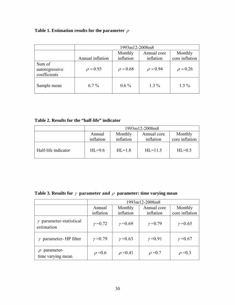
Table 1. Estimation results for the parameter ρ

1993m12-2008m8

Annual inflation Monthly inflation

Annual core inflation

Monthly core inflation

Sum of autoregressive coefficients

=ρ 0.93 =ρ 0.68 =ρ 0.94 =ρ 0.26

Sample mean

6.7 % 0.6 % 1.3 % 1.5 %

Table 2. Results for the “half-life” indicator

1993m12-2008m8

Annual inflation

Monthly inflation

Annual core inflation

Monthly core inflation

Half-life indicator HL=9.6 HL=1.8 HL=11.5 HL=0.5

Table 3. Results for γ parameter and ρ parameter: time varying mean

1993m12-2008m8

Annual inflation

Monthly inflation

Annual core inflation

Monthly core inflation

γ parameter-statistical estimation

γ =0.72 γ =0.69 γ =0.79 γ =0.65

γ parameter- HP filter γ =0.79 γ =0.63 γ =0.91 γ =0.67

ρ parameter- time varying mean

ρ =0.6 ρ =0.41 ρ =0.7 ρ =0.3

30

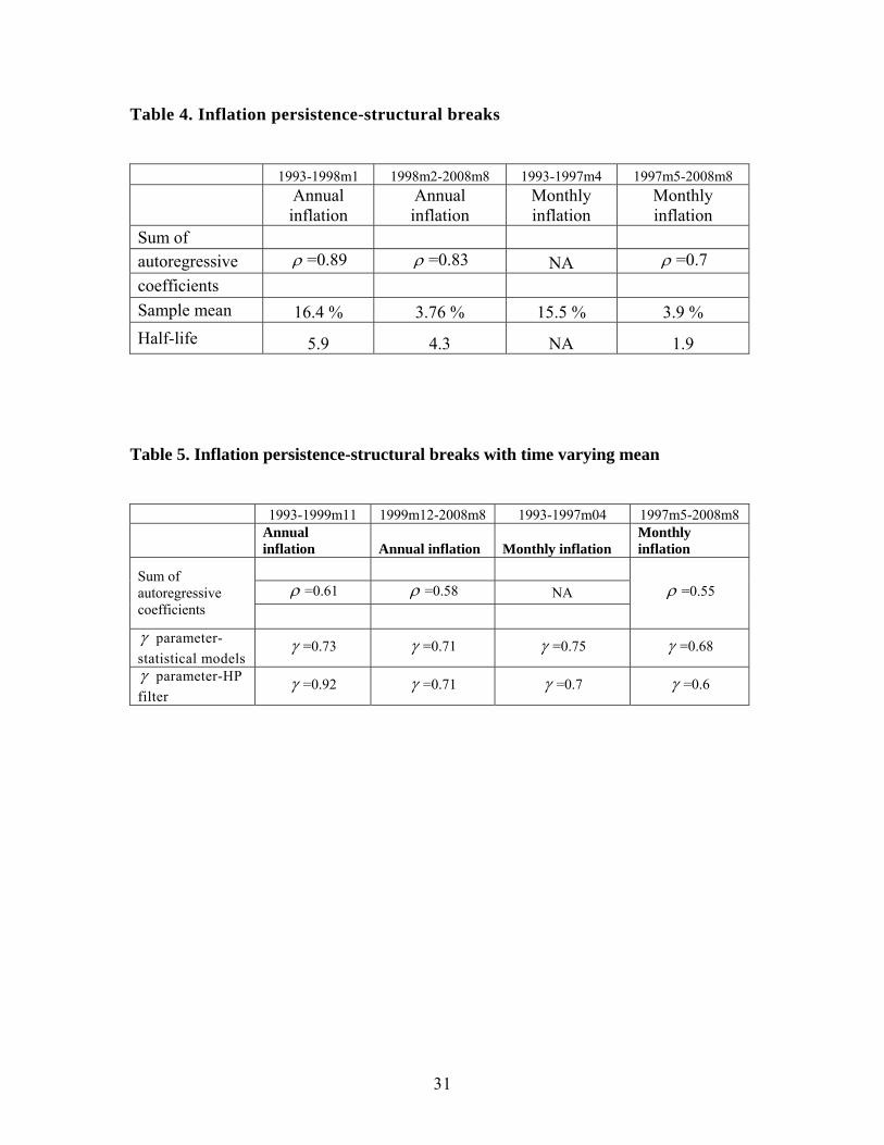
Table 4. Inflation persistence-structural breaks

1993-1998m1 1998m2-2008m8 1993-1997m4 1997m5-2008m8

Annual inflation

Annual inflation

Monthly inflation

Monthly inflation

Sum of autoregressive ρ =0.89 ρ =0.83 NA ρ =0.7 coefficients Sample mean 16.4 % 3.76 % 15.5 % 3.9 % Half-life 5.9 4.3 NA 1.9

Table 5. Inflation persistence-structural breaks with time varying mean

1993-1999m11 1999m12-2008m8 1993-1997m04 1997m5-2008m8

Annual inflation Annual inflation Monthly inflation

Monthly inflation

ρ =0.61 ρ =0.58 NA

Sum of autoregressive coefficients

ρ =0.55

γ parameter-statistical models

γ =0.73 γ =0.71 γ =0.75 γ =0.68

γ parameter-HP filter

γ =0.92 γ =0.71 γ =0.7 γ =0.6

31

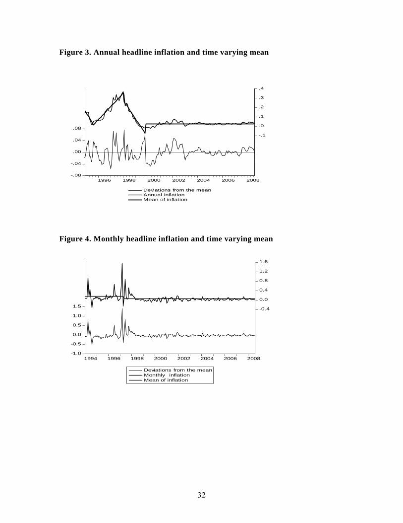
Figure 3. Annual headline inflation and time varying mean

-.08

-.04

.00

.04

.08

-.1

.0

.1

.2

.3

.4

1996 1998 2000 2002 2004 2006 2008

Deviations from the meanAnnual inflationMean of inflation

Figure 4. Monthly headline inflation and time varying mean

-1.0

-0.5

0.0

0.5

1.0

1.5 -0.4

0.0

0.4

0.8

1.2

1.6

1994 1996 1998 2000 2002 2004 2006 2008

Deviations from the meanMonthly inflationMean of inflation

32

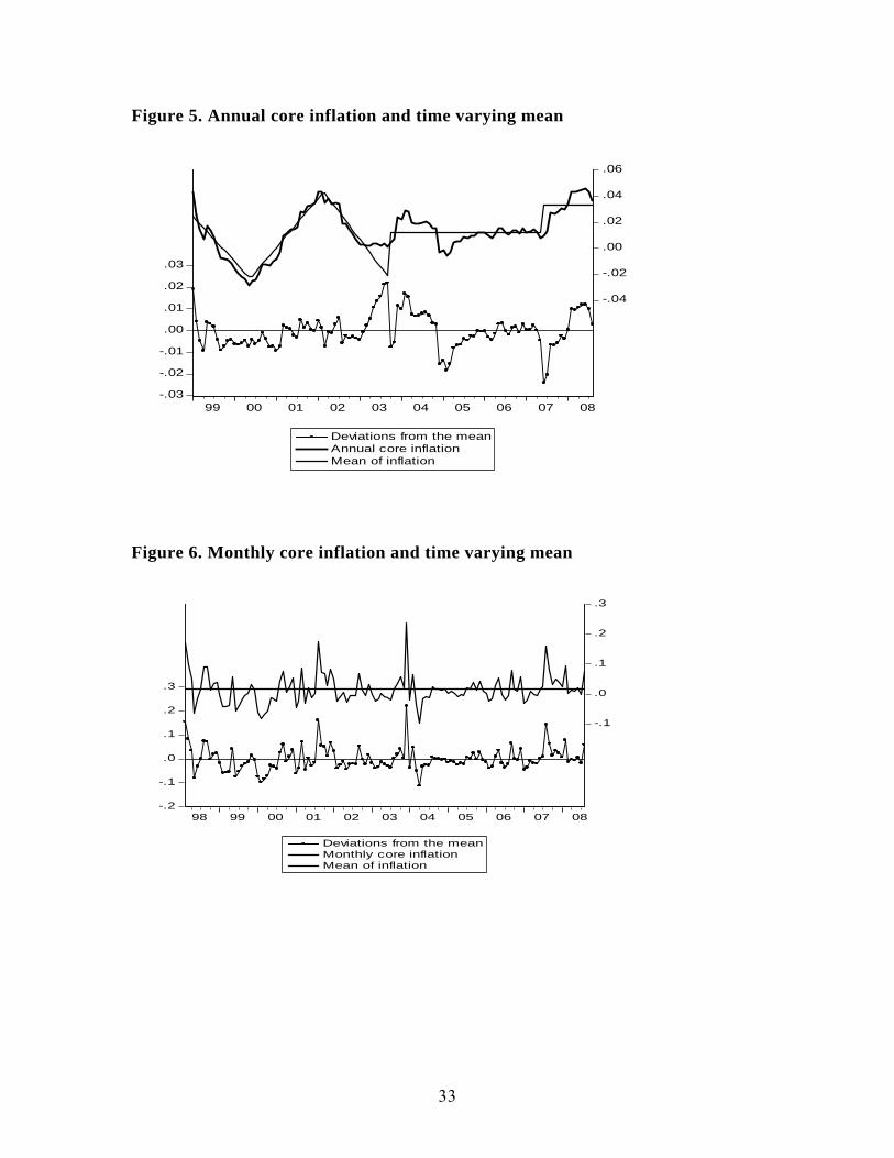
Figure 5. Annual core inflation and time varying mean

-.03

-.02

-.01

.00

.01

.02

.03

-.04

-.02

.00

.02

.04

.06

99 00 01 02 03 04 05 06 07 08

Deviations from the meanAnnual core inflationMean of inflation

Figure 6. Monthly core inflation and time varying mean

-.2

-.1

.0

.1

.2

.3

-.1

.0

.1

.2

.3

98 99 00 01 02 03 04 05 06 07 08

Deviations from the meanMonthly core inflationMean of inflation

33

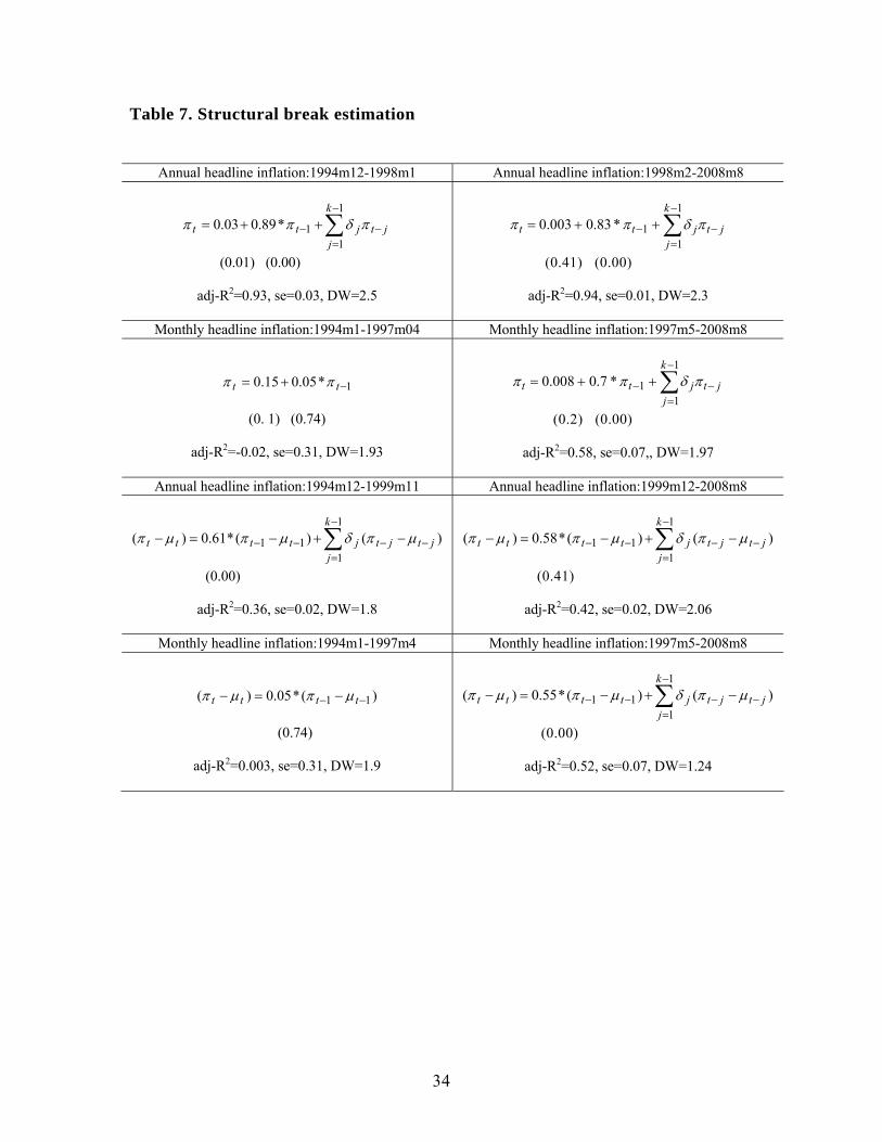
Table 7. Structural break estimation

Annual headline inflation:1994m12-1998m1 Annual headline inflation:1998m2-2008m8

∑−

=−− ++=

1

11*89.003.0

k

jjtjtt πδππ

(0.01) (0.00)

adj-R2=0.93, se=0.03, DW=2.5

∑−

=−− ++=

1

11*83.0003.0

k

jjtjtt πδππ

(0.41) (0.00)

adj-R2=0.94, se=0.01, DW=2.3

Monthly headline inflation:1994m1-1997m04 Monthly headline inflation:1997m5-2008m8

1*05.015.0 −+= tt ππ

(0. 1) (0.74)

adj-R2=-0.02, se=0.31, DW=1.93

∑−

=−− ++=

1

11*7.0008.0

k

jjtjtt πδππ

(0.2) (0.00)

adj-R2=0.58, se=0.07,, DW=1.97

Annual headline inflation:1994m12-1999m11 Annual headline inflation:1999m12-2008m8

)()(*61.0)(1

111 jt

k

jjtjtttt −

−

=−−− −+−=− ∑ µπδµπµπ

(0.00)

adj-R2=0.36, se=0.02, DW=1.8

)()(*58.0)(1

111 jt

k

jjtjtttt −

−

=−−− −+−=− ∑ µπδµπµπ

(0.41)

adj-R2=0.42, se=0.02, DW=2.06

Monthly headline inflation:1994m1-1997m4 Monthly headline inflation:1997m5-2008m8

)(*05.0)( 11 −− −=− tttt µπµπ

(0.74)

adj-R2=0.003, se=0.31, DW=1.9

)()(*55.0)(1

111 jt

k

jjtjtttt −

−

=−−− −+−=− ∑ µπδµπµπ

(0.00)

adj-R2=0.52, se=0.07, DW=1.24

34

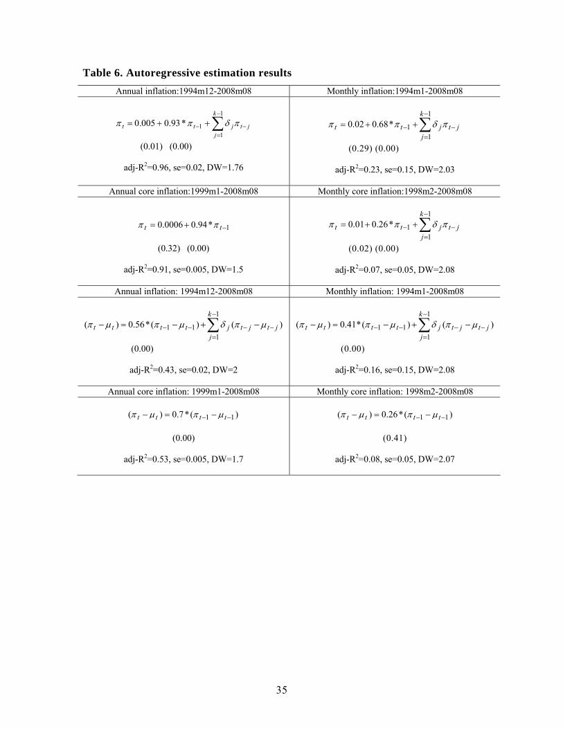
Table 6. Autoregressive estimation results Annual inflation:1994m12-2008m08 Monthly inflation:1994m1-2008m08

∑−

=−− ++=

1

11*93.0005.0

k

jjtjtt πδππ

(0.01) (0.00)

adj-R2=0.96, se=0.02, DW=1.76

∑−

=−− ++=

1

11*68.002.0

k

jjtjtt πδππ

(0.29) (0.00)

adj-R2=0.23, se=0.15, DW=2.03

Annual core inflation:1999m1-2008m08 Monthly core inflation:1998m2-2008m08

1*94.00006.0 −+= tt ππ

(0.32) (0.00)

adj-R2=0.91, se=0.005, DW=1.5

∑−

=−− ++=

1

11*26.001.0

k

jjtjtt πδππ

(0.02) (0.00)

adj-R2=0.07, se=0.05, DW=2.08

Annual inflation: 1994m12-2008m08 Monthly inflation: 1994m1-2008m08

)()(*56.0)(1

111 jt

k

jjtjtttt −

−

=−−− −+−=− ∑ µπδµπµπ

(0.00)

adj-R2=0.43, se=0.02, DW=2

)()(*41.0)(1

111 jt

k

jjtjtttt −

−

=−−− −+−=− ∑ µπδµπµπ

(0.00)

adj-R2=0.16, se=0.15, DW=2.08

Annual core inflation: 1999m1-2008m08 Monthly core inflation: 1998m2-2008m08

)(*7.0)( 11 −− −=− tttt µπµπ

(0.00)

adj-R2=0.53, se=0.005, DW=1.7

)(*26.0)( 11 −− −=− tttt µπµπ

(0.41)

adj-R2=0.08, se=0.05, DW=2.07

35

36

Discussion Sophia Lazaretou2

Bank of Greece

The paper by Vasilika Kota on ‘the persistence of inflation in Albania’ is an

informative and useful one. I really enjoyed reading it. It is rich both in narrative

and empirical evidence on the time series properties of the inflation process in

Albania.

Up to now, the received empirical literature, dealing mainly with the US, the

UK and the euro area, suggests that inflation persistence may not be an intrinsic

structural phenomenon of industrial countries ‘but rather varies with the stability

and transparency of the monetary policy’ (Levin and Piger 2004, p6). Therefore, the

paper does enrich our knowledge on the relationship between monetary policy

regimes and the behaviour of inflation in emerging market economies.

Let start my discussion briefly summarizing the methodology used and the key

empirical findings. The author presents an assessment of inflation persistence over

the period 1993-2008. To this end, she uses three alternative measures: (i) by

looking at the autocorrelation properties of inflation; (ii) by measuring the number

of periods that a shock needs before its effects are reduced by 50 per cent; and (iii)

by determining the mean properties of inflation. The assessment is produced by

using both a constant and a time varying estimation of mean inflation. The existence

of possible shifts in inflation persistence is also examined. Two measures of

inflation are equally considered, core and headline, and inflation is measured both

on an annual and a monthly basis.

The empirical findings reveal that inflation in Albania persists. Analytically,

the data detect a significant shift both in inflation persistence and its mean rate

across the two monetary regimes, implying that the monetary regime does matter.

2 Economic Research Department. Email: slazaretou@bankofgreece.gr.

37

Core inflation is shown to be more persistent than headline inflation whereas

monthly inflation rates exhibit lower persistence compared to annual rates.

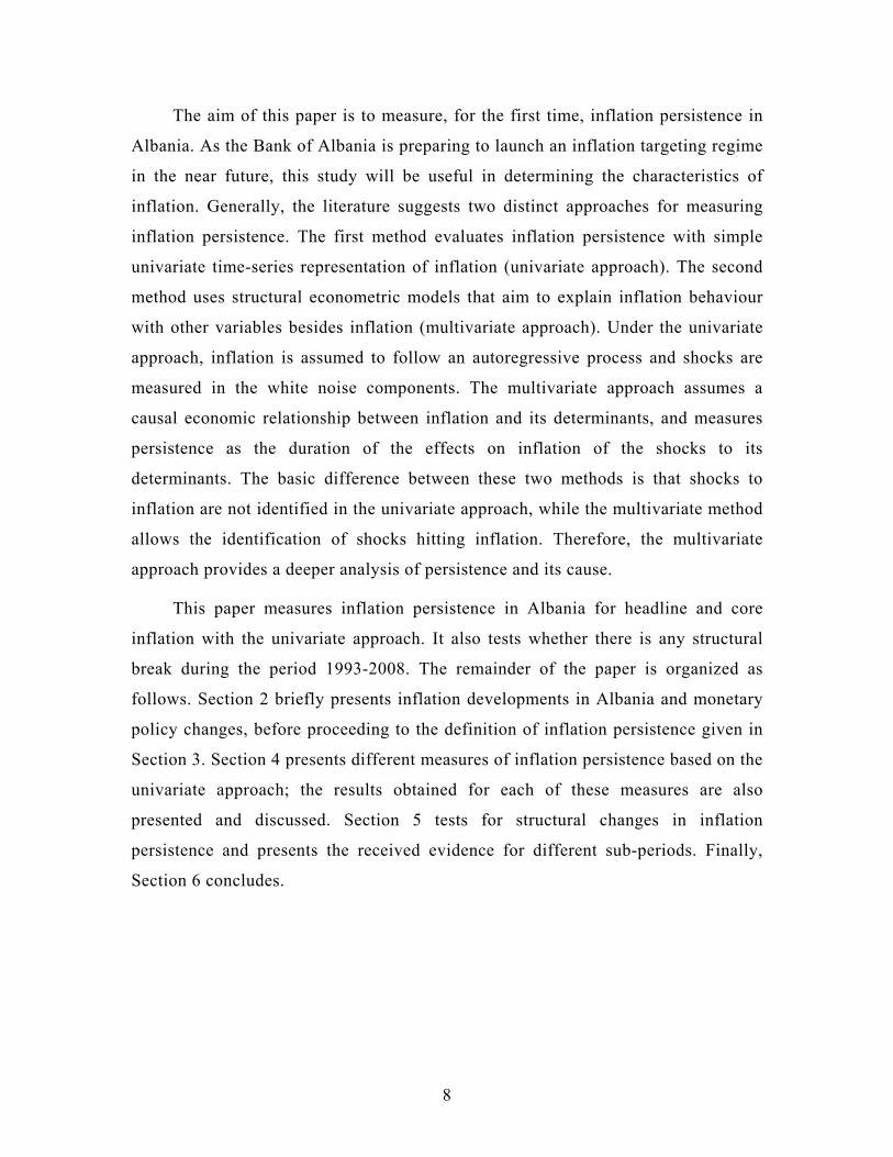
My first comment concerns the meaning of persistence. Figure 1 depicts the

evolution over time of the inflation process. Simple inspection reveals that three

distinct phases can be easily detected: (i) an inflationary period up to 1997; (ii) a

dis-inflationary period up to 2000 and (iii) a period of price stability afterwards. It is

evident that Albania is a country with a high variance of inflation and has

experienced a variety of policy regimes that might have affected the behaviour of

the inflation process both in the sense of the steady state inflation rate and its

autocorrelation properties. Therefore, the meaning of inflation persistence across

different phases is different.

A key question is thus addressed: What does persistence mean? In philosophy,

persistence means the condition of enduring in time, with or without change. In

biotechnology, it means the ability of an organism to remain in a particular setting

for a period of time after it is introduced. In environmental health and toxicology, it

is the attribute of a substance that describes the length of time that the substance

remains in a particular environment before it is physically removed or chemically or

biologically transformed.

In economics, however, persistence has both positive and normative aspects.

Referring to the positive aspects, typical measures of inflation persistence are (see

Batini 2002, Batini and Nelson 2001): (i) positive serial correlation; (ii) the length

of the delay between a systematic monetary policy action and its peak effect on

inflation; and (iii) the lagged inflation response to a monetary policy shock.

Referring to normative aspects, however, inflation persistence does not have the

same connotation in periods of high inflation as in periods of disinflation or in

periods of price stability (see Hondroyiannis and Lazaretou 2007). A negative

connotation is associated with high inflation rates accompanied by a high inflation

in the future, thus producing a vicious circle. A positive connotation is associated

with persistence in disinflation periods. It means that the inertia of inflationary

expectations breaks down and inflation is steadily falling, thus producing a virtuous

circle. In periods of low and stable inflation rates, inflation does not persist while

38

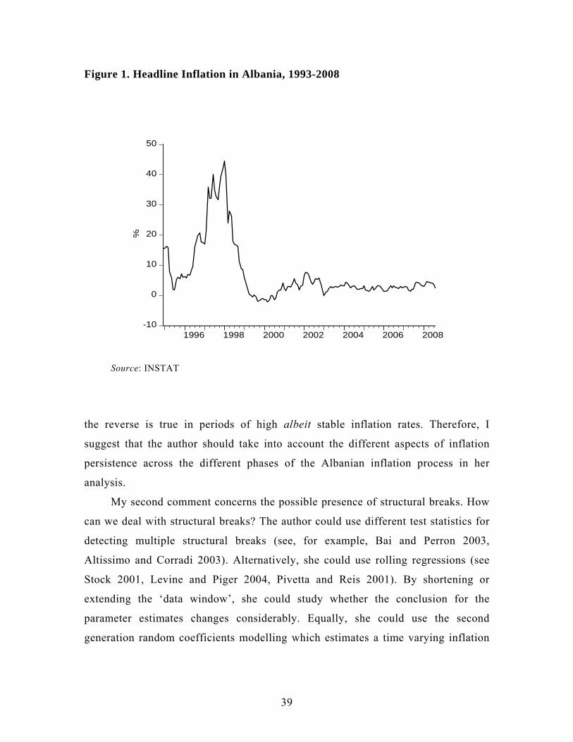
Figure 1. Headline Inflation in Albania, 1993-2008

-10

0

10

20

30

40

50

1996 1998 2000 2002 2004 2006 2008

%

Source: INSTAT

the reverse is true in periods of high albeit stable inflation rates. Therefore, I

suggest that the author should take into account the different aspects of inflation

persistence across the different phases of the Albanian inflation process in her

analysis.

My second comment concerns the possible presence of structural breaks. How

can we deal with structural breaks? The author could use different test statistics for

detecting multiple structural breaks (see, for example, Bai and Perron 2003,

Altissimo and Corradi 2003). Alternatively, she could use rolling regressions (see

Stock 2001, Levine and Piger 2004, Pivetta and Reis 2001). By shortening or

extending the ‘data window’, she could study whether the conclusion for the

parameter estimates changes considerably. Equally, she could use the second

generation random coefficients modelling which estimates a time varying inflation

39

persistence and relaxes specifications such as a specific functional form (Swammy

and Tavlas 2001).

More importantly, my third comment focuses on monetary policy making.

From the point of view of monetary policy making, it is important first to

distinguish between a change in monetary policy stance (systematic monetary policy

action) and a monetary policy shock (non-systematic) and, second, try to determine

whether and how much the response of inflation has changed following changes in

the monetary policy framework.

Closing this short discussion, I would like to mention two topics for further

research. First, it might be useful to present evidence looking at price data on a

sectoral level rather on an aggregated level. This will explain whether the cross-

sectional variation in persistence and in the steady state of inflation can be

determined by the structural features of different sectors. This type of analysis is of

great importance since cross country emerging market evidence is of acute interest

for policy decision making. Explicitly, it helps us in validating results and

explaining cross country differences.

Second, a different approach to studying inflation persistence is to estimate a

reduced form model of inflation with time varying parameters, employing a

methodology akin to Beechey and Österholn (2007), Cogley et al. (2010) and

Angeloni et al. (2006). Within this framework, time variation in inflation

persistence is motivated as reflecting changes in the relative weight on output gap

deviations in the central bank’s loss function. Based on this approach, it has been

found that inflation persistence in advanced economies declined post-1999. This

decline might have stemmed from changes in central bank preferences.

40

References Altissimo, F. and V. Corradi (2003), ‘Strong Rules for Detecting the Number of Breaks in a Time Series’, Journal of Econometrics, 207-244. Angeloni, I., C. Aucremanne and M. Ciccarelli (2006), ‘Price Setting and Inflation Persistence: Did EMU Matter’, Economic Policy, 46, 353-387. Bai, J. and E. Perron (2003), ‘Estimating and Testing Linear Models with Multiple Structural Changes’, Econometrica, 47-78. Batini, N, (2002), ‘Euro Area Inflation Persistence’, ECB Working Paper no 201. Batini, N. and E. Nelson (2001), ‘The Lag from Monetary Policy Actions to Inflation: Friedman Revisited’, International Finance, 381-400. Beechey, T. and P. Österholn (2007), ‘The Rise and the Fall of US Inflation Persistence’, Finance and Economics Discussion Series, 26, Board of Governors of the Federal Reserve System. Cogley, T., G. E. Primiceri and T. J. Sargent (2010), ‘Inflation-Gap Persistence in the US’, American Economic Journal: Macroeconomy, 2, 43-69. Hondroyiannis, G. and S. Lazaretou (2007), ‘Inflation Persistence during Periods of Structural Change: an assessment using Greek data’, Empirica, 34, 453-475. Levin, A. T. and Piger, J.M. (2004), ‘Is Inflation Persistence Intrinsic in Industrial Economies?’, ECB Working Paper, no 334. Pivetta, F. and R. Reis (2001), ‘The Persistence of Inflation in the US’, mimeo, Harvard University. Stock, J. (2001) ‘Comment on Evolving post-WWII US Inflation Dynamics’, NBER Macroeconomis Annual, 379-387. Swammy, P.A.V.B. and G. Tavlas (2001), ‘Random Coefficient Models’, in Baltagi, B. H. (ed.) Companion to Theoretical Econometrics, Basil Blackwell, Oxford, 410-428.

41

42

Special Conference Papers

3rd South-Eastern European Economic Research Workshop Bank of Albania-Bank of Greece

Athens, 19-21 November 2009

1. Hardouvelis, Gikas, Keynote address: “The World after the Crisis: S.E.E. Challenges & Prospects”, February 2011.

2. Tanku, Altin “Another View of Money Demand and Black Market Premium Relationship: What Can They Say About Credibility?”, February 2011.

3. Kota, Vasilika “The Persistence of Inflation in Albania”, including discussion by Sophia Lazaretou, February 2011.

4. Kodra, Oriela “Estimation of Weights for the Monetary Conditions Index in Albania”, including discussion by Michael Loufir, February 2011.

5. Pisha, Arta “Eurozone Indices: A New Model for Measuring Central Bank Independence”, including discussion by Eugenie Garganas, February 2011.

6. Kapopoulos, Panayotis and Sophia Lazaretou “International Banking and Sovereign Risk Calculus: the Experience of the Greek Banks in SEE”, including discussion by Panagiotis Chronis, February 2011.

7. Shijaku, Hilda and Kliti Ceca “A Credit Risk Model for Albania” including discussion by Faidon Kalfaoglou, February 2011.

8. Kalluci, Irini “Analysis of the Albanian Banking System in a Risk-Performance Framework”, February 2011.

9. Georgievska, Ljupka, Rilind Kabashi, Nora Manova-Trajkovska, Ana Mitreska, Mihajlo Vaskov “Determinants of Lending Rates and Interest Rate Spreads”, including discussion by Heather D. Gibson, February 2011.

10. Kristo, Elsa “Being Aware of Fraud Risk”, including discussion by Elsida Orhan, February 2011.

11. Malakhova, Tatiana “The Probability of Default: a Sectoral Assessment", including discussion by Vassiliki Zakka, February 2011.

12. Luçi, Erjon and Ilir Vika “The Equilibrium Real Exchange Rate of Lek Vis-À-Vis Euro: Is It Much Misaligned?”, including discussion by Dimitrios Maroulis, February 2011.

13. Dapontas, Dimitrios “Currency Crises: The Case of Hungary (2008-2009) Using Two Stage Least Squares”, including discussion by Claire Giordano, February 2011.

43