β3-IRT: A New Item Response Model and its Applications

Yu Chen Telmo Silva FilhoUniversity of Bristol Universidade Federal de Pernambuco

Ricardo B. C. Prudêncio Tom Diethe Peter FlachUniversidade Federal de Pernambuco Amazon University of Bristol & Alan Turing Institute

Abstract

Item Response Theory (IRT) aims to assess latentabilities of respondents based on the correctnessof their answers in aptitude test items with dif-ferent difficulty levels. In this paper, we proposethe β3-IRT model, which models continuous re-sponses and can generate a much enriched familyof Item Characteristic Curves. In experiments weapplied the proposed model to data from an onlineexam platform, and show our model outperformsa more standard 2PL-ND model on all datasets.Furthermore, we show how to apply β3-IRT toassess the ability of machine learning classifiers.This novel application results in a new metric forevaluating the quality of the classifier’s probabil-ity estimates, based on the inferred difficulty anddiscrimination of data instances.

1 INTRODUCTION

IRT is widely adopted in psychometrics for estimating hu-man latent ability in tests. Unlike classical test theory, whichis concerned with performance at the test level, IRT focuseson the items, modelling responses given by respondentswith different abilities to items of different difficulties, bothmeasured in a known scale [Embretson and Reise, 2013].The concept of item depends on the application, and canrepresent for instance test questions, judgements or choicesin exams. In practice, IRT models estimate latent difficultiesof the items and the latent abilities of the respondents basedon observed responses in a test, and have been commonlyapplied to assess performance of students in exams.

Recently, IRT was adopted to analyse Machine Learning

Proceedings of the 22nd International Conference on Artificial In-telligence and Statistics (AISTATS) 2019, Naha, Okinawa, Japan.PMLR: Volume 89. Copyright 2019 by the author(s).

(ML) classification tasks [Martínez-Plumed et al., 2016].Here, items correspond to instances in a dataset, while re-spondents are classifiers. The responses are the outcomesof classifiers on the test instances (right or wrong decisionscollected in a cross-validation experiment). Our work isdifferent in two aspects: 1) we propose a new IRT modelfor continuous responses; 2) we applied the proposed IRTto predicted probabilities instead of binary responses.

For each item (instance), an Item Characteristic Curve (ICC)is estimated, which is a logistic function that returns theprobability of a correct response for the item based onthe respondent ability. This ICC is determined by twoitem parameters: difficulty, which is the location param-eter of the logistic function; and discrimination, whichaffects the slope of the ICC. Despite the useful insights[Martínez-Plumed et al., 2016] and applicability to otherAI contexts, binary IRT models are limited when the tech-niques of interest return continuous responses (e.g. classprobabilities). Continuous IRT models have been developedand applied in psychometrics [Noel and Dauvier, 2007] buthave limitations when applied in this context: limited inter-pretability since abilities and difficulties are expressed asreal numbers; and limited flexibility since ICCs are limitedto logistic functions.

In this paper, we propose a novel IRT model called β3-IRTto addresses these limitations by means of a new parameteri-sation of IRT models such that: a) the resulting ICCs are notlimited to logistic curves, different shapes can be obtaineddepending on the item parameters, which allows more flexi-bility when fitting responses for different items; b) abilitiesand difficulties are in the [0, 1] range, which gives a unifiedscale for easier interpretation and evaluation.

We first applied the β3-IRT model in a case studyto predict students’ responses in an online educationplatform. Out model outperforms the 2PL-ND model[Noel and Dauvier, 2007] on all datasets. In a second casestudy, β3-IRT was used to fit class probabilities estimatedby classifiers in binary classification tasks. The experimen-tal results show the ability inferred by the model allows to

β3-IRT: A New Item Response Model and its Applications

evaluate probability estimation of classifiers in an instance-wise manner with the aid of item parameters (difficulty anddiscrimination). Hence we show that the β3-IRT model isuseful not only in the more traditional applications associ-ated with IRT, but also in the ML context outlined above.

Our contributions can be summarised as follows:

• we propose a new model for IRT with richer ICCshapes, which is more versatile than existing models;

• we demonstrate empirically that this model has betterpredictive power;

• we demonstrate the use of this model in an ML setting,providing a method for assessing the ‘ability’ of clas-sification algorithms that is based on an instance-wisemetric in terms of class probability estimation.

The paper is organised as follows. Section 2 gives a briefintroduction of Binary Item Response Theory (IRT). Sec-tion 3 presents the β3-IRT model, followed by related workon IRT in Section 3.3. Section 4 presents the experiments onreal students, while Section 5 presents the use of β3-IRT toevaluate classifiers. Finally, Section 6 concludes the paper.

2 BINARY ITEM-RESPONSE THEORY

In Item Response Theory, the probability of a correct re-sponse for an item depends on the latent respondent abilityand the item difficulty. Most previous studies on IRT haveadopted binary models, in which the responses are eithercorrect or incorrect. Such models assume a binary responsexij of the i-th respondent to the j-th item. In the IRT modelwith two item parameters (2PL), the probability of a correctresponse (xij = 1) is defined by a logistic function withlocation parameter δj and shape parameter aj . Responsesare modelled by the Bernoulli distribution with parameterpij as follows:

xij = Bern(pij), pij = σ(−ajdij), dij = θi − δj (1)

where σ(·) is the logistic function. N is the number of itemsand M is the number of participants.

The 2PL model gives a logistic Item Characteristic Curve(ICC) mapping ability θi to expected response as follows:

E[xij |θi, δj ,aj ] = pij =1

1 + e−aj(θi−δj)(2)

At θi = δj the expected response is 0.5. The slope ofthe ICC at θi = δj is aj/4. If aj = 1,∀j = 1, . . . , N , asimpler model is obtained, known as 1PL, which describesitems solely by their difficulties. Generally, discriminationaj indicates how probability of correct responses changesas the ability increases. High discriminations lead to steepICCs at the point where ability equals difficulty, with small

pij

Beta

αij βij

θi δj aj

Beta(1, 1) Beta(1, 1) N (1, σ20)

Fα Fβ

M N

6

Figure 1: Factor Graph of β3-IRT Model. The grey circle repre-sents observed data, white circles represent latent variables, smallblack rectangles represent stochastic factors, and the rectangularplates represent replicates.

changes in ability producing significant changes in the prob-ability of correct response.

The standard IRT model implicitly uses a noise model thatfollows a logistic distribution (in the same way that logisticregression does). This can be replaced with Normally dis-tributed noise, which results in the logistic link function be-ing replaced by a probit link function (Gaussian CumulativeDistribution Function (CDF)), as is the case in the DAREmodel [Bachrach et al., 2012]. In practice, the probit linkfunction is very similar to the logistic one, so these twomodels tend to behave very similarly, and the particularchoice is often then based on mathematical convenience orcomputation tractability.

Despite their extensive use in psychometrics, binary IRTmodels are of limited use when responses are naturallyproduced in continuous scales. Particularly in ML, binarymodels are not adequate if the responses to evaluate areclass probability estimates.

3 THE β3-IRT MODEL

In this Section, we will elaborate on the parametrisationand inference method of β3-IRT model, highlighting thedifferences with existing IRT models.

3.1 Model description

The factor graph of β3-IRT is shown in Fig 1 and Eq (3)below gives the model definition, where M is number ofrespondents and N is number of items, pij is the observedresponse of respondent i to item j, which is drawn from a

Yu Chen, Telmo Silva Filho, Ricardo B. C. Prudêncio, Tom Diethe, Peter Flach

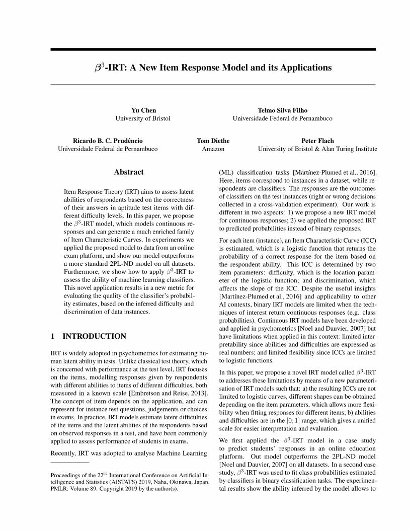
(a) aj = 2. (b) aj = 1. (c) aj = 0.5.

Figure 2: Examples of Beta ICCs for Different Values of Difficulty and Discrimination. Higher discriminations lead to steeper ICCs,higher difficulties need higher abilities to achieve higher responses.

Beta distribution:

pij ∼ B(αij , βij),

αij = Fα(θi, δj ,aj) =

(θiδj

)aj

,

βij = Fβ(θi, δj ,aj) =

(1− θi1− δj

)aj

,

θi ∼ B(1, 1), δj ∼ B(1, 1), aj ∼ N (1, σ20) (3)

The parameters αij , βij are computed from θi (the abilityof participant i), δj (the difficulty of item j), and aj (thediscrimination of item j). θi and δj are also drawn fromBeta distributions and their priors are set to B(1, 1) in ageneral setting. The discrimination aj is drawn from a Nor-mal distribution with prior mean 1 and variance σ2

0 , whereσ0 is a hyperparameter of the model. These uninformativepriors are used as default setting of the model, but couldbe parametrised by further hyperparameters when there isfurther prior information available. The default prior meanof aj is set to 1 rather than 0 because the discrimination ajis a power factor here.

When comparing probabilities we use ratios (e.g. the like-lihood ratio). Similarly, here we use the ratio of ability todifficulty since in our model these are measured on a [0, 1]scale as well: a ratio smaller/larger than 1 means that abilityis lower/higher than difficulty. These ratios are positive realsand hence map directly to α and β in Eq (3). Importantly,the new parametrisation enables us to obtain non-logisticICCs. In this model the ICC is defined by the expectationof B(αij , βij) and then assumes the form:

E[pij |θi, δj ,aj ] =αij

αij + βij=

1

1 +(

δj

1−δj

)aj(

θi

1−θi

)−aj

(4)

As in standard IRT, the difficulty δj is a location parameter.The response is 0.5 when θi = δj and the curve has slope

aj/(4δj(1 − δj)) at that point. Fig 2 shows examples ofBeta ICCs for different regimes depending on aj :

aj > 1 : a sigmoid shape similar to stardard IRT,aj = 1 : parabolic curves with vertex at 0.5,

0 <aj < 1 : anti-sigmoidal behaviour.

Note that the model allows for negative discrimination,which indicates items that are somehow harder for moreable respondents. Negative aj can be divided similarly:

−1 <aj < 0 : decreasing anti-sigmoid,aj < 1 : decreasing sigmoid.

We will see examples in Section 5 that negative discrimi-nation can in fact be useful for identifying ‘noisy’ items,where higher abilities getting lower responses.

3.2 Model inference

We tested two inference methods on β3-IRT model, one isconventional Maximum Likelihood (MLE) which we ap-plied to experiments with student answers (Section 4) forresponse prediction, using the likelihood function shown inEq (4).

The other is Bayesian Variational Inference (VI)[Bishop, 2006] which we applied to experiments withclassifiers (Section 5) for full Bayesian inference on latentvariables. In VI, the optimisation objective is the lowerbound of Kullback–Leibler (KL) divergence between thetrue posterior and variational posterior of latent variables,which is also referred as Evidence Lower Bound (ELBO).However, the model is highly non-identifiable because of itssymmetry [Nishihara et al., 2013], resulting in undesirablecombinations of these variables: for instance, when pij isclose to 1, it usually indicates αij > 1 and βij < 1, whichcan arise when θi > δj with positive aj , or θi < δj withnegative aj . Hence, we update discrimination as a global

β3-IRT: A New Item Response Model and its Applications

Algorithm 1: Variational Inference for β3-IRT

1 Set number of iterations Liter, randomly initialise φ,ψ, λ;2 for t in range(Liter) do3 while Θ = {φ,ψ} not converged do4 Compute∇ΘL1 according to Eq (5);5 Update Θ by SGD;6 end7 Compute∇λL2 according to Eq (6);8 Update λ by SGD;9 end

variable after ability and difficulty converge at each step(see also Algorithm 1), in addition to setting the prior ofdiscrimination as N(1,1) to reflect the assumption thatdiscrimination is more often positive than negative. We em-ploy the coordinate ascent method of VI [Blei et al., 2017],keeping aj fixed while optimising θi and δj and vice versa.Accordingly, the two separate loss functions are defined asbelow:

L1 =

M∑i=1

N∑j=1

Eq[log p(pij |θi, δj)]

+

M∑i=1

Eq[log p(θi)− log q(θi|φi)]

+

N∑j=1

Eq[log p(δj)− log q(δj |ψj)] (5)

L2 =

N∑j=1

Eq[log p(pij |aj)+log p(aj)−log q(aj |λj)] (6)

Here, φ,ψ,λ are parameters of variational posteriors ofθ, δ,a, respectively. L1 and L2 are lower bounds ofKL(p(θ, δ|x)||q(θ, δ|φ,ψ)) and KL(p(a|x)||q(a|λ), re-spectively. Both are optimised using Stochastic GradientDescent (SGD). In order to apply the reparameterisationtrick [Kingma and Welling, 2013], we use Logit-Normal toapproximate the Beta distribution in variational posteriors.The steps to perform VI of the model are shown in Algo-rithm 1, where the variational parameters can be updatedby any gradient descent optimisation algorithm (we use theAdam method [Kingma and Ba, 2014] in our experiments).We implemented Algorithm 1 using the probabilistic pro-gramming library Edward [Tran et al., 2016].

3.3 Related work

There have been earlier approaches to IRT with continuousapproaches. In particular, [Noel and Dauvier, 2007] pro-posed an IRT model which adopts the Beta distribution with

parameters mij and nij as follows:

mij = e(θi−δj)/2, nij = e−(θi−δj)/2 = m−1ij ,

pij ∼ B(mij , nij).

This model gives a logistic ICC mapping ability to expectedresponse for item j of the form:

E[pij |θi, δj ] =mij

mij + nij=

1

1 + e−(θi−δj)(7)

While there is a superficial similarity to the β3-IRT model,there are two crucial distinctions.

• Similarly to the standard 1PL IRT model, Eq (7) doesnot have a discrimination parameter. The ICC thereforehas a fixed slope of 0.25 at θi = δj and it is assumedthat all items have the same discrimination.

• Eq (7) assumes a real-valued scale for abilities and dif-ficulties, whereas β3-IRT uses a [0, 1] scale. Not onlydoes this avoid problems with interpreting extremevalues, but more importantly it opens the door to thenon-sigmoidal ICCs as depicted in Figure 2.

4 EXPERIMENTS WITH STUDENTANSWER DATASETS

We begin by applying and evaluating β3-IRT to model re-sponses of students, which is a common application of IRT.We use datasets that consist of answers given by studentsof 33 different courses from an online platform (which wecannot disclose, for commercial reasons). The courses havedifferent numbers of questions, but not all students haveanswered all questions for a given course (in fact, most didnot), therefore we did not have pij values for every student iand question j. On the other hand, it is possible for a studentto answer a question multiple times. These datasets maycontain noise derived from user behaviour, such as quicklyanswering questions just to see the next ones and lendingaccounts to other students.

We compare the β3-IRT model with Noel and Dauvier’scontinuous IRT model. Since without a discrimination pa-rameter their model is rather weak, we strengthen it byintroducing a discrimination parameter as follows:

E[pij |θi, δj ,aj ] =mij

mij + nij=

1

1 + e−aj(θi−δj)(8)

We refer to this model as 2PL-ND.

Our experiments follow two scenarios. In the first sce-nario, to generate the continuous responses, we take thei-th student’s average performance for the j-th question,pij = E[xij ]. In the second scenario, only the first attemptsof each student for each question are considered, leading to

Yu Chen, Telmo Silva Filho, Ricardo B. C. Prudêncio, Tom Diethe, Peter Flach

−3 −2 −1 0 1 2 3 4 5 6 70

0.2

0.4

0.6

0.8

1

Discrimination

Diffi

culty

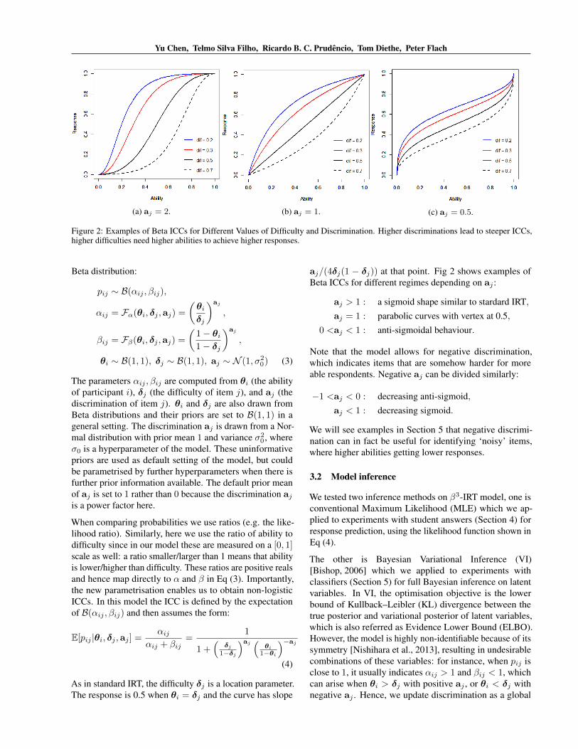
Figure 3: Discrimination versus Difficulty (Inferred in one ofthe 30 hold-out schemes across all 33 student answer datasets.Solid dots represent discriminations in the (−1, 1) range, whichproduce non-logistic curves in our approach. These representapproximately 46% of all estimated discriminations.)

a binary problem. The models were trained by minimisingthe log-loss of predicted probabilities using SGD, imple-mented in Python, with the Theano library. We trained themodels for 2500 iterations, using batches of 2000 answersand an adaptive learning rate calculated as 0.5/

√t, where

t is the current iteration. β3-IRT predicts the probabilitythat the i-th student will answer the j-th question correctlyfollowing Eq (4), while 2PL-ND follows Eq (8).

For 2PL-ND, abilities and difficulties are unbounded anddrawn from N (0, 1). For β3-IRT, abilities are boundedin the range (0, 1), so they were drawn from B(m+

i ,m−i ),

were m+i (m−

i ) represent the number of correct (incorrect)answers given by the i-th student. Likewise, difficultieswere drawn from B(n+

j , n−j ), where n+

j (n−j ) represent thenumber of correct (incorrect) answers given to the j-th ques-tion. For both models, discriminations were drawn fromN (1, 1).

In the experiments, we ran 30 hold-out schemes with 90%of the dataset kept for training and 10% for testing. Fora training set to be valid, every student and question mustoccur in it at least once. Therefore, we sample the trainingand test sets with stratification based on the students andthen we check which questions are absent, sampling 90%of their answers for training and 10% for testing.

Table 1 shows the log-loss for all 33 courses (full details ofthese courses can be found in the supplementary material).Best results were marked in bold, in case they were statisti-cally significant according to a paired Wilcoxon signed-ranktest, with significance level 0.001. The results show thatβ3-IRT outperformed 2PL-ND in all cases. We posit thatthis can be explained by the versatility of the model, whichis able to find non-logistic ICCs when discriminations aretaken from (−1, 1). Fig 3 shows that roughly 46% of allquestions from the 33 datasets are estimated to have dis-

Table 1: Student Answer Datasets (Log-loss) for Continuous (Stu-dent’s Average) and First Attempt Performance.

continuous first attempts

course β3-IRT 2PL-ND β3-IRT 2PL-ND

1 0.631 ± 0.003 0.713 ± 0.004 0.623 ± 0.004 0.699 ± 0.0052 0.630 ± 0.022 0.972 ± 0.081 0.623 ± 0.023 0.953 ± 0.0603 0.617 ± 0.004 0.695 ± 0.004 0.628 ± 0.024 0.760 ± 0.0864 0.671 ± 0.004 0.742 ± 0.009 0.669 ± 0.004 0.731 ± 0.0075 0.594 ± 0.004 0.692 ± 0.008 0.597 ± 0.004 0.696 ± 0.0136 0.661 ± 0.009 0.899 ± 0.039 0.651 ± 0.009 0.892 ± 0.0307 0.630 ± 0.007 0.795 ± 0.020 0.632 ± 0.007 0.791 ± 0.0158 0.648 ± 0.014 0.941 ± 0.044 0.641 ± 0.023 0.967 ± 0.0599 0.657 ± 0.011 0.941 ± 0.030 0.660 ± 0.011 0.931 ± 0.03210 0.649 ± 0.007 0.847 ± 0.030 0.655 ± 0.009 0.841 ± 0.03211 0.633 ± 0.016 0.889 ± 0.051 0.630 ± 0.012 0.891 ± 0.06712 0.650 ± 0.013 0.938 ± 0.063 0.662 ± 0.016 0.883 ± 0.05113 0.697 ± 0.066 1.002 ± 0.218 0.659 ± 0.086 1.023 ± 0.42314 0.642 ± 0.028 0.936 ± 0.074 0.623 ± 0.028 0.909 ± 0.05715 0.588 ± 0.002 0.650 ± 0.003 0.584 ± 0.003 0.642 ± 0.00316 0.605 ± 0.002 0.674 ± 0.003 0.603 ± 0.002 0.663 ± 0.00217 0.603 ± 0.002 0.665 ± 0.003 0.596 ± 0.003 0.657 ± 0.00318 0.598 ± 0.006 0.725 ± 0.008 0.608 ± 0.005 0.729 ± 0.01119 0.651 ± 0.015 0.923 ± 0.064 0.644 ± 0.020 0.934 ± 0.07420 0.640 ± 0.021 0.959 ± 0.060 0.636 ± 0.018 0.933 ± 0.04021 0.639 ± 0.016 0.949 ± 0.072 0.650 ± 0.014 0.968 ± 0.09422 0.629 ± 0.020 0.935 ± 0.050 0.622 ± 0.016 0.931 ± 0.06023 0.602 ± 0.004 0.692 ± 0.011 0.609 ± 0.004 0.682 ± 0.00524 0.657 ± 0.014 0.950 ± 0.046 0.652 ± 0.011 0.950 ± 0.04425 0.642 ± 0.015 0.917 ± 0.034 0.627 ± 0.010 0.871 ± 0.03826 0.572 ± 0.011 0.836 ± 0.045 0.593 ± 0.014 0.874 ± 0.03827 0.662 ± 0.022 0.998 ± 0.093 0.647 ± 0.028 0.971 ± 0.07328 0.603 ± 0.001 0.647 ± 0.002 0.603 ± 0.001 0.645 ± 0.00229 0.553 ± 0.021 0.916 ± 0.056 0.558 ± 0.017 0.856 ± 0.05130 0.646 ± 0.019 1.001 ± 0.075 0.647 ± 0.019 0.979 ± 0.04831 0.647 ± 0.014 0.911 ± 0.060 0.634 ± 0.014 0.918 ± 0.05332 0.578 ± 0.001 0.627 ± 0.001 0.578 ± 0.002 0.626 ± 0.00233 0.663 ± 0.021 0.929 ± 0.060 0.674 ± 0.025 0.993 ± 0.074

criminations in this interval, supporting this conclusion. Asshown in Fig 2c, non-logistic ICCs are better at discrimi-nating lower and higher ability values than logistic ICCs,which focus more on ability values around the correspond-ing question difficulty, and β3-IRT is able to model bothcases. Additionally, approximately 10% of all questionshad negative discriminations. One possible explanation isthe presence of noise in these datasets, as mentioned earlierin this section. We will return to the relationship betweennegative discrimination and noise in Section 5.

5 β3-IRT FOR CLASSIFIERS

We now apply β3-IRT to supervised machine learning. Here,each ‘respondent’ is a different classifier and items are in-stances from a classification dataset1. The responses arethe probabilities of the correct class assigned by the classi-fiers to each instance. Specifically, the observed response isgiven by pij =

∑k I(yj = k)pijk, where I(·) is the indica-

tor function, yj is the label of item j, k is the index of eachclass, and pijk is the predicted probability of item j fromclass k given by classifier i. The application of β3-IRT inclassification tasks aims to answer the following:

1. Can item parameters be used to characterise instancesin terms of: (i) how difficult it is to estimate classprobabilities for each instance; and (ii) how useful

1Note that an entire dataset could be considered as an item too,with associated difficulty.

β3-IRT: A New Item Response Model and its Applications

−2 −1 0 1 2 3 4 5 6

−1

0

1

2

3

4

5

6

δ (Difficulty)

−2 −1 0 1 2 3 4 5 6

−1

0

1

2

3

4

5

6

a (Discrimination)

0.0 0.1 0.2 0.3 0.4 0.5 0.6 0.7 0.80

2

4

6

8

Histogram of δ

−1.0 −0.5 0.0 0.5 1.0 1.5 2.00.0

0.5

1.0

1.5

2.0

Histogram of a

IRT item parameters

(a) Dataset CLUSTERS

−1.0 −0.5 0.0 0.5 1.0 1.5 2.0

−0.4

−0.2

0.0

0.2

0.4

0.6

0.8

1.0

δ (Difficulty)

−1.0 −0.5 0.0 0.5 1.0 1.5 2.0

−0.4

−0.2

0.0

0.2

0.4

0.6

0.8

1.0

a (Discrimination)

0.1 0.2 0.3 0.4 0.5 0.6 0.70

2

4

6

8

10

Histogram of δ

−1.0 −0.5 0.0 0.5 1.0 1.50.0

0.5

1.0

1.5

2.0

2.5

Histogram of a

IRT item parameters

(b) Dataset MOONS.

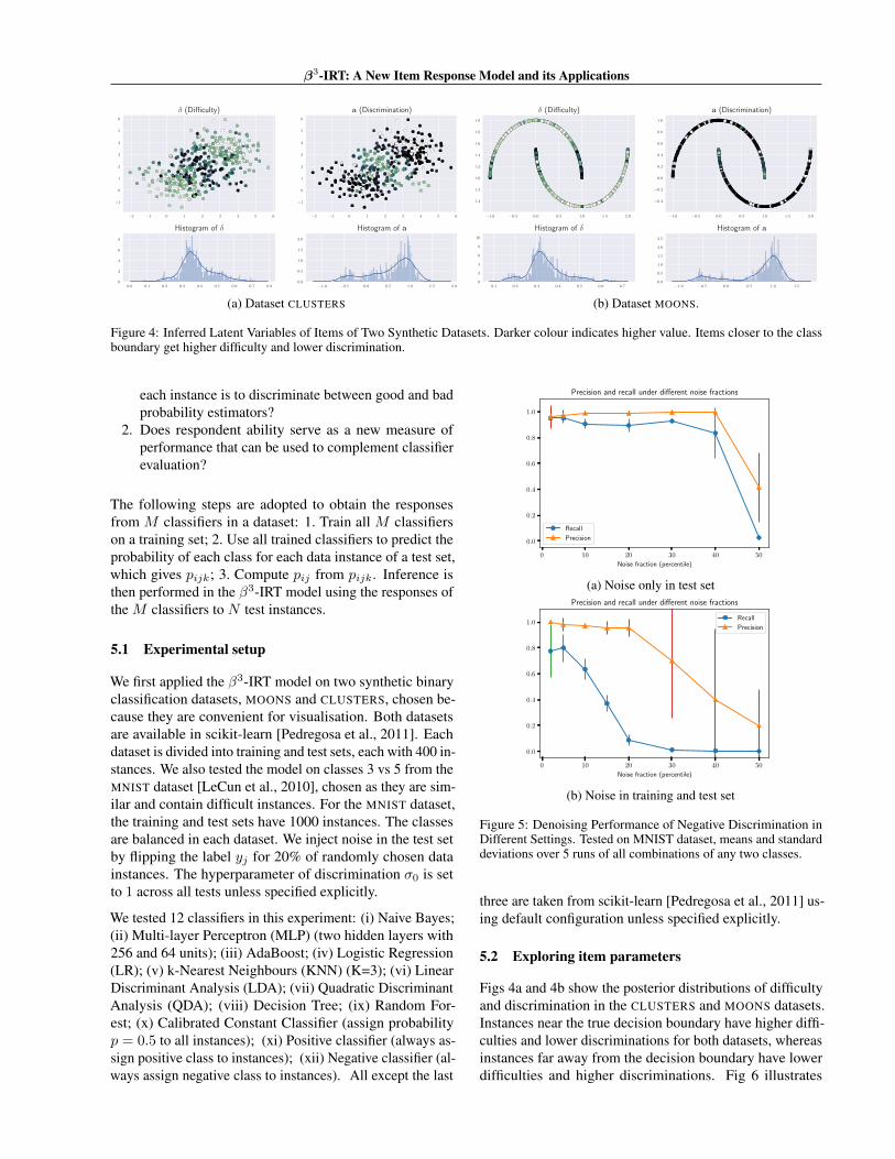
Figure 4: Inferred Latent Variables of Items of Two Synthetic Datasets. Darker colour indicates higher value. Items closer to the classboundary get higher difficulty and lower discrimination.

each instance is to discriminate between good and badprobability estimators?

2. Does respondent ability serve as a new measure ofperformance that can be used to complement classifierevaluation?

The following steps are adopted to obtain the responsesfrom M classifiers in a dataset: 1. Train all M classifierson a training set; 2. Use all trained classifiers to predict theprobability of each class for each data instance of a test set,which gives pijk; 3. Compute pij from pijk. Inference isthen performed in the β3-IRT model using the responses ofthe M classifiers to N test instances.

5.1 Experimental setup

We first applied the β3-IRT model on two synthetic binaryclassification datasets, MOONS and CLUSTERS, chosen be-cause they are convenient for visualisation. Both datasetsare available in scikit-learn [Pedregosa et al., 2011]. Eachdataset is divided into training and test sets, each with 400 in-stances. We also tested the model on classes 3 vs 5 from theMNIST dataset [LeCun et al., 2010], chosen as they are sim-ilar and contain difficult instances. For the MNIST dataset,the training and test sets have 1000 instances. The classesare balanced in each dataset. We inject noise in the test setby flipping the label yj for 20% of randomly chosen datainstances. The hyperparameter of discrimination σ0 is setto 1 across all tests unless specified explicitly.

We tested 12 classifiers in this experiment: (i) Naive Bayes;(ii) Multi-layer Perceptron (MLP) (two hidden layers with256 and 64 units); (iii) AdaBoost; (iv) Logistic Regression(LR); (v) k-Nearest Neighbours (KNN) (K=3); (vi) LinearDiscriminant Analysis (LDA); (vii) Quadratic DiscriminantAnalysis (QDA); (viii) Decision Tree; (ix) Random For-est; (x) Calibrated Constant Classifier (assign probabilityp = 0.5 to all instances); (xi) Positive classifier (always as-sign positive class to instances); (xii) Negative classifier (al-ways assign negative class to instances). All except the last

0 10 20 30 40 50

Noise fraction (percentile)

0.0

0.2

0.4

0.6

0.8

1.0

Precision and recall under different noise fractions

Recall

Precision

(a) Noise only in test set

0 10 20 30 40 50

Noise fraction (percentile)

0.0

0.2

0.4

0.6

0.8

1.0

Precision and recall under different noise fractions

Recall

Precision

(b) Noise in training and test set

Figure 5: Denoising Performance of Negative Discrimination inDifferent Settings. Tested on MNIST dataset, means and standarddeviations over 5 runs of all combinations of any two classes.

three are taken from scikit-learn [Pedregosa et al., 2011] us-ing default configuration unless specified explicitly.

5.2 Exploring item parameters

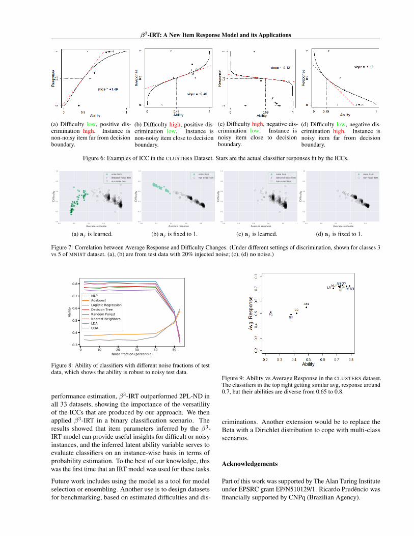
Figs 4a and 4b show the posterior distributions of difficultyand discrimination in the CLUSTERS and MOONS datasets.Instances near the true decision boundary have higher diffi-culties and lower discriminations for both datasets, whereasinstances far away from the decision boundary have lowerdifficulties and higher discriminations. Fig 6 illustrates

Yu Chen, Telmo Silva Filho, Ricardo B. C. Prudêncio, Tom Diethe, Peter Flach

ICCs for different combinations of difficulty, discrimina-tion and ability. Our model provides more flexibility thanlogistic-shape ICC.

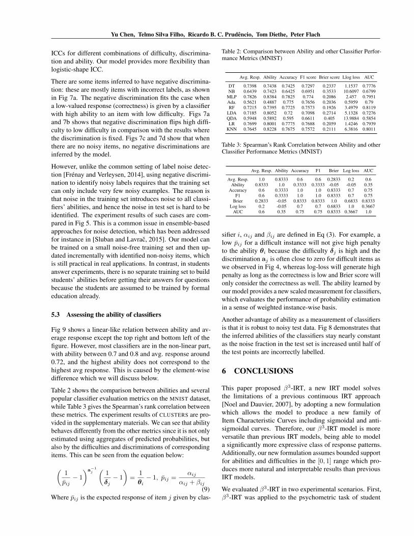
There are some items inferred to have negative discrimina-tion: these are mostly items with incorrect labels, as shownin Fig 7a. The negative discrimination fits the case whena low-valued response (correctness) is given by a classifierwith high ability to an item with low difficulty. Figs 7aand 7b shows that negative discrimination flips high diffi-culty to low difficulty in comparison with the results wherethe discrimination is fixed. Figs 7c and 7d show that whenthere are no noisy items, no negative discriminations areinferred by the model.

However, unlike the common setting of label noise detec-tion [Frénay and Verleysen, 2014], using negative discrimi-nation to identify noisy labels requires that the training setcan only include very few noisy examples. The reason isthat noise in the training set introduces noise to all classi-fiers’ abilities, and hence the noise in test set is hard to beidentified. The experiment results of such cases are com-pared in Fig 5. This is a common issue in ensemble-basedapproaches for noise detection, which has been addressedfor instance in [Sluban and Lavrac, 2015]. Our model canbe trained on a small noise-free training set and then up-dated incrementally with identified non-noisy items, whichis still practical in real applications. In contrast, in studentsanswer experiments, there is no separate training set to buildstudents’ abilities before getting their answers for questionsbecause the students are assumed to be trained by formaleducation already.

5.3 Assessing the ability of classifiers

Fig 9 shows a linear-like relation between ability and av-erage response except the top right and bottom left of thefigure. However, most classifiers are in the non-linear part,with ability between 0.7 and 0.8 and avg. response around0.72, and the highest ability does not correspond to thehighest avg response. This is caused by the element-wisedifference which we will discuss below.

Table 2 shows the comparison between abilities and severalpopular classifier evaluation metrics on the MNIST dataset,while Table 3 gives the Spearman’s rank correlation betweenthese metrics. The experiment results of CLUSTERS are pro-vided in the supplementary materials. We can see that abilitybehaves differently from the other metrics since it is not onlyestimated using aggregates of predicted probabilities, butalso by the difficulties and discriminations of correspondingitems. This can be seen from the equation below:

(1

pij− 1

)a−1j(

1

δj− 1

)=

1

θi− 1, pij =

αijαij + βij

(9)Where pij is the expected response of item j given by clas-

Table 2: Comparison between Ability and other Classifier Perfor-mance Metrics (MNIST)

Avg. Resp. Ability Accuracy F1 score Brier score Llog loss AUC

DT 0.7398 0.7438 0.7425 0.7297 0.2337 1.1537 0.7776NB 0.6439 0.7423 0.6425 0.6951 0.3533 10.6097 0.6799

MLP 0.7826 0.8384 0.7825 0.774 0.2086 2.457 0.7951Ada. 0.5621 0.4887 0.775 0.7656 0.2036 0.5959 0.79RF 0.7215 0.7395 0.7725 0.7573 0.1926 3.4979 0.8119

LDA 0.7185 0.8052 0.72 0.7098 0.2714 5.1328 0.7276QDA 0.5948 0.5892 0.595 0.6611 0.405 13.9884 0.5854LR 0.7699 0.8001 0.7775 0.7688 0.2059 1.4246 0.7939

KNN 0.7645 0.8228 0.7675 0.7572 0.2111 6.3816 0.8011

Table 3: Spearman’s Rank Correlation between Ability and otherClassifier Performance Metrics (MNIST)

Avg. Resp. Ability Accuracy F1 Brier Log loss AUC

Avg. Resp. 1.0 0.8333 0.6 0.6 0.2833 0.2 0.6Ability 0.8333 1.0 0.3333 0.3333 -0.05 -0.05 0.35

Accuracy 0.6 0.3333 1.0 1.0 0.8333 0.7 0.75F1 0.6 0.3333 1.0 1.0 0.8333 0.7 0.75

Brier 0.2833 -0.05 0.8333 0.8333 1.0 0.6833 0.8333Log loss 0.2 -0.05 0.7 0.7 0.6833 1.0 0.3667

AUC 0.6 0.35 0.75 0.75 0.8333 0.3667 1.0

sifier i, αij and βij are defined in Eq (3). For example, alow pij for a difficult instance will not give high penaltyto the ability θi because the difficulty δj is high and thediscrimination aj is often close to zero for difficult items aswe observed in Fig 4, whereas log-loss will generate highpenalty as long as the correctness is low and Brier score willonly consider the correctness as well. The ability learned byour model provides a new scaled measurement for classifiers,which evaluates the performance of probability estimationin a sense of weighted instance-wise basis.

Another advantage of ability as a measurement of classifiersis that it is robust to noisy test data. Fig 8 demonstrates thatthe inferred abilities of the classifiers stay nearly constantas the noise fraction in the test set is increased until half ofthe test points are incorrectly labelled.

6 CONCLUSIONS

This paper proposed β3-IRT, a new IRT model solvesthe limitations of a previous continuous IRT approach[Noel and Dauvier, 2007], by adopting a new formulationwhich allows the model to produce a new family ofItem Characteristic Curves including sigmoidal and anti-sigmoidal curves. Therefore, our β3-IRT model is moreversatile than previous IRT models, being able to modela significantly more expressive class of response patterns.Additionally, our new formulation assumes bounded supportfor abilities and difficulties in the [0, 1] range which pro-duces more natural and interpretable results than previousIRT models.

We evaluated β3-IRT in two experimental scenarios. First,β3-IRT was applied to the psychometric task of student

β3-IRT: A New Item Response Model and its Applications

(a) Difficulty low, positive dis-crimination high. Instance isnon-noisy item far from decisionboundary.

(b) Difficulty high, positive dis-crimination low. Instance isnon-noisy item close to decisionboundary.

(c) Difficulty high, negative dis-crimination low. Instance isnoisy item close to decisionboundary.

(d) Difficulty low, negative dis-crimination high. Instance isnoisy item far from decisionboundary.

Figure 6: Examples of ICC in the CLUSTERS Dataset. Stars are the actual classifier responses fit by the ICCs.

0.0 0.2 0.4 0.6 0.8 1.0

Average response

0.0

0.2

0.4

0.6

0.8

1.0

Diffi

cult

y

Correlation between difficulty and response

noise item

detected noise item

non-noise item

(a) aj is learned.

0.0 0.2 0.4 0.6 0.8 1.0

Average response

0.0

0.2

0.4

0.6

0.8

1.0

Diffi

cult

y

Correlation between difficulty and response

noise item

non-noise item

(b) aj is fixed to 1.

0.0 0.2 0.4 0.6 0.8 1.0

Average response

0.0

0.2

0.4

0.6

0.8

1.0

Diffi

cult

y

Correlation between difficulty and response

noise item

detected noise item

non-noise item

(c) aj is learned.

0.0 0.2 0.4 0.6 0.8 1.0

Average response

0.0

0.2

0.4

0.6

0.8

1.0

Diffi

cult

y

Correlation between difficulty and response

noise item

non-noise item

(d) aj is fixed to 1.

Figure 7: Correlation between Average Response and Difficulty Changes. (Under different settings of discrimination, shown for classes 3vs 5 of MNIST dataset. (a), (b) are from test data with 20% injected noise; (c), (d) no noise.)

0 10 20 30 40 50Noise fraction (percentile)

0.3

0.4

0.5

0.6

0.7

0.8

Abilit

y

MLPAdaboostLogistic RegressionDecision TreeRandom ForestNearest NeighborsLDAQDA

Figure 8: Ability of classifiers with different noise fractions of testdata, which shows the ability is robust to noisy test data.

performance estimation, β3-IRT outperformed 2PL-ND inall 33 datasets, showing the importance of the versatilityof the ICCs that are produced by our approach. We thenapplied β3-IRT in a binary classification scenario. Theresults showed that item parameters inferred by the β3-IRT model can provide useful insights for difficult or noisyinstances, and the inferred latent ability variable serves toevaluate classifiers on an instance-wise basis in terms ofprobability estimation. To the best of our knowledge, thiswas the first time that an IRT model was used for these tasks.

Future work includes using the model as a tool for modelselection or ensembling. Another use is to design datasetsfor benchmarking, based on estimated difficulties and dis-

Figure 9: Ability vs Average Response in the CLUSTERS dataset.The classifiers in the top right getting similar avg, response around0.7, but their abilities are diverse from 0.65 to 0.8.

criminations. Another extension would be to replace theBeta with a Dirichlet distribution to cope with multi-classscenarios.

Acknowledgements

Part of this work was supported by The Alan Turing Instituteunder EPSRC grant EP/N510129/1. Ricardo Prudêncio wasfinancially supported by CNPq (Brazilian Agency).

Yu Chen, Telmo Silva Filho, Ricardo B. C. Prudêncio, Tom Diethe, Peter Flach

References

[Bachrach et al., 2012] Bachrach, Y., Minka, T., Guiver, J.,and Graepel, T. (2012). How to grade a test withoutknowing the answers: a Bayesian graphical model foradaptive crowdsourcing and aptitude testing. In Proc. ofthe 29th Int. Conf. on Machine Learning, pages 819–826.Omnipress.

[Bishop, 2006] Bishop, C. M. (2006). Pattern Recognitionand Machine Learning. Springer.

[Blei et al., 2017] Blei, D. M., Kucukelbir, A., andMcAuliffe, J. (2017). Variational inference: A review forstatisticians. Journal of the American Statistical Associa-tion, 112(518):859–877.

[Embretson and Reise, 2013] Embretson, S. and Reise, S.(2013). Item Response Theory for Psychologists. Taylor& Francis.

[Frénay and Verleysen, 2014] Frénay, B. and Verleysen, M.(2014). Classification in the presence of label noise:a survey. IEEE transactions on neural networks andlearning systems, 25(5):845–869.

[Kingma and Ba, 2014] Kingma, D. and Ba, J. (2014).Adam: A method for stochastic optimization. In Proc. ofthe 3rd Int. Conf. on Learning Representations (ICLR).

[Kingma and Welling, 2013] Kingma, D. P. and Welling,M. (2013). Auto-encoding variational Bayes. In Proc. ofthe 2nd Int. Conf. on Learning Representations (ICLR).

[LeCun et al., 2010] LeCun, Y., Cortes, C., and Burges,C. J. (2010). MNIST handwritten digit database.AT&T Labs [Online]. Available: http://yann. lecun.com/exdb/mnist, 2.

[Martínez-Plumed et al., 2016] Martínez-Plumed, F.,Prudêncio, R. B., Martínez-Usó, A., and Hernández-Orallo, J. (2016). Making sense of item responsetheory in machine learning. In European Conference onArtificial Intelligence, ECAI, pages 1140–1148.

[Nishihara et al., 2013] Nishihara, R., Minka, T., and Tar-low, D. (2013). Detecting parameter symmetries in prob-abilistic models. arXiv preprint arXiv:1312.5386.

[Noel and Dauvier, 2007] Noel, Y. and Dauvier, B. (2007).A beta item response model for continuous bounded re-sponses. Applied Psychological Measurement, 31(1):47–73.

[Pedregosa et al., 2011] Pedregosa, F., Varoquaux, G.,Gramfort, A., Michel, V., Thirion, B., Grisel, O., Blondel,M., Prettenhofer, P., Weiss, R., Dubourg, V., Vanderplas,J., Passos, A., Cournapeau, D., Brucher, M., Perrot, M.,and Duchesnay, E. (2011). Scikit-learn: Machine learn-ing in Python. Journal of Machine Learning Research,12:2825–2830.

[Sluban and Lavrac, 2015] Sluban, B. and Lavrac, N.(2015). Relating ensemble diversity and performance: Astudy in class noise detection. Neurocomputing, 160:120–131.

[Tran et al., 2016] Tran, D., Kucukelbir, A., Dieng, A. B.,Rudolph, M., Liang, D., and Blei, D. M. (2016). Ed-ward: A library for probabilistic modeling, inference,and criticism. arXiv preprint arXiv:1610.09787.