Validated Continuation Over Large Parameter

Ranges for Equilibria of PDEs

Marcio Gameiro ∗ Jean-Philippe Lessard†

Konstantin Mischaikow‡

Abstract

Validated continuation was introduced in [4] as means of checking thatthe classical continuation method applied to a Galerkin projection of aPDE provides a locally unique equilibrium to the PDE of interest. In thispaper we extend the numerical technique to include a parameter that leadsto better bounds on the errors associated with the Galerkin truncation.We test this method on the Swift-Hohenberg and Allen-Cahn equationson one dimensional domains. For the first equation, we find no numericalobstructions to the validated continuation technique. This is not the casefor the Allen-Cahn equation.

1 Introduction

The question of finding zeros of a nonlinear function arises in many mathemat-ical domains. In the setting of a one parameter family of nonlinear differentialequations

ut = f(u, ν), u ∈ H, ν ∈ R, (1)

defined on a Hilbert space H , the zeros correspond to equilibria. If f is a suf-ficiently smooth function, then the set of equilibria E := (u, ν) | f(u, ν) = 0is, at least locally, typically a smooth curve in H × R. In this case, continua-tion provides a particularly efficient manner of approximating E . Recall, thatthis method involves a predictor and corrector step: given, within a prescribed

∗Department of Mathematics, Rutgers University, 110 Frelinghusen Rd, Piscataway, NJ08854-8019, USA (gameiro@math.rutgers.edu). The author was partially supported by grantsfrom D.O.E. and DARPA.

†School of Mathematics, Georgia Institute of Technology, Atlanta, Georgia 30332-0160USA (lessard@math.gatech.edu). The author was partially supported by FQRNT, NSFDMS 0511115 and grants from D.O.E. and DARPA. Currently visiting: Department of Math-ematics, Rutgers University, 110 Frelinghusen Rd, Piscataway, NJ 08854-8019, USA

‡Department of Mathematics, Hill Center-Busch Campus, Rutgers, The State Univer-sity of New Jersey, 110 Frelinghusen Rd, Piscataway, NJ 08854-8019, USA and Schoolof Mathematics, Georgia Institute of Technology, Atlanta, Georgia 30332-0160 USA(mischaik@math.rutgers.edu). The author was partially supported by NSF DMS 0511115and grants from D.O.E. and DARPA.

1

tolerance, an equilibrium u0 at parameter value ν0, the predictor step producesan approximate equilibrium u1 at nearby parameter value ν1, and the correctorstep, often based on a Newton-like operator, takes u1 as its input and produces,once again within the prescribed tolerance, an equilibrium u1 at ν1.

Our interest is in the case where (1) is a partial differential equation, andhence, H is an infinite dimensional space. Thus, to perform the continuationdescribed above requires a priori reducing the infinite dimensional problem toa finite dimensional system, this often involves a Galerkin projection. A funda-mental implication of this is that while the continuation method may succeed,it is not clear that the solution closely approximates elements of E . To addressthis problem, the concept of validated continuation was introduced in [4].

To review the essential elements of validated continuation assume that (1)takes the form

ut = L(u, ν) +d∑

p=0

cp(ν)up (2)

where u is scalar, L(·, ν) is a linear operator at parameter value ν, and d is thedegree of the polynomial nonlinearity. Typically, c1(ν) = 0 since linear termsare grouped under L(·, ν). Using an appropriate Fourier series expansion of (2)results in a countable system of differential equations on the coefficients of theexpanded solution, which for the sake of simplicity we assume takes the form

uk = fk(u, ν) := µkuk +

d∑

p=0

∑

P

ni=k

(cp)n0un1 · · ·unp , k = 0, 1, 2, . . . (3)

where µk = µk(ν) are the parameter dependent eigenvalues of L(·, ν) and unand (cp)n are the coefficients of the corresponding expansions of the functionsu and cp(ν) respectively with un = u−n and (cp)n = (cp)−n for all n.

The continuation method is applied to the m-dimensional system of ordinarydifferential equations

uk = µkuk +

d∑

p=0

∑

P

ni=k

|ni|<m

(cp)n0un1 · · ·unp , k = 0, 1, . . . , m − 1 (4)

obtained from (3) via a Galerkin projection. The validation technique providesjustification that the numerical approximations of equilibria of (4) are satisfac-tory approximations of the equilibria of (2).

The theoretical basis for the validation technique is provided by the Ba-nach fixed point theorem: A contraction mapping T : X → X on a completemetric space has a unique fixed point in X. Observe that in a neighborhoodof a hyperbolic fixed point the Newton operator is a contraction mapping thatprovides super linear convergence. Furthermore, the not insignificant compu-tational cost of deriving a numerical Newton-like operator is performed in thecontinuation step. Thus, for the sake of efficiency the validation technique fo-cuses on efficiently determining the set X on which a controlled perturbation ofthe numerical operator is a contraction mapping.

2

We apply the validated continuation technique to parabolic PDEs for whichthe equilibria are smooth, that is they are C∞ in x. We exploit this smoothnessand assume that we can express the set X in the form Wu(r) where u is anumerical zero obtained from the continuation method applied to (4) and

Wu(r) = u +

m−1∏

k=0

[−r, r] ×

∞∏

k=m

[

−As

ks,As

ks

]

. (5)

As the notation suggests, we think of s and As as constants and r, the validationradius, as a variable to be solved for. In particular, as is described in Section 2,r is taken to be a solution to a set of polynomial inequalities which encode thetruncation errors associated with performing the continuation technique on theprojection of Wu(r) to

∏m−1k=0 [−r, r].

Two important points of [4] are the following: (1) if the validation radiusr exists, then the Banach fixed point theorem applies and hence there exists aunique equilibrium in the set Wu(r), and (2) the cost of validated continuationis comparable with that of the standard continuation applied to (4). In order tofocus on the essential elements of the validated continuation technique, severalobvious numerical improvements and questions were explicitly left undevelopedin [4, Section 7]. We turn to two of these issues in this paper.

1. Observe that if (2) has a polynomial nonlinearity of order d, then straight-forward evaluation of the nonlinear term in (4) involves on the order ofmd operations. This computational cost can be reduced by making use ofFast Fourier Transform (FFT) techniques.

2. As is mentioned above, the truncation of Wu(r) to∏m−1

k=0 [−r, r] introduceserrors that must be overcome in order to solve for a validation radius. Thesimple assumption that |uk| ≤

As

ks for all k ≥ m provides a computation-ally cheap, but large, bound on the error. Though computationally moreexpensive, it is shown in [4] that the bounds can be improved by using ex-plicit constraints on |uk| for k = m, . . . , M for some M ≥ m. For the sakeof clarity the computations performed in [4] were restricted to M = m.In this paper we exploit the computational parameter M to carry outcontinuation for large ranges of parameter values.

This paper is organized as follows. Establishing that an operator T is acontraction mapping on a space X is a question of estimates. This is addressedin Section 2. In particular, after introducing some notation the results of [4] arerecalled in Section 2.1. As is mentioned above, given m, M is a computationalparameter that is used to control the size of truncation errors. In Section 2.2we provide a lower bound on the choice of M . In Section 2.3, we indicate howthe FFT can be used to compute the nonlinear sums. In Section 3, we applyour techniques to two model problems: the Swift-Hohenberg equation and theAllen-Cahn equation. Finally, in Section 4 we use the results of our numericalexperiments to suggest future directions of research.

3

2 Essential Estimates

Throughout the paper, we will use the subscript (·)F to denote the componentsk ∈ 0, · · · , m − 1. Recall that following the expansion of the system in theappropriate basis, we have

u = f(u, ν) (6)

whose component-wise expansion is given by (3). Let m be a fixed projectiondimension and consider the following truncation of (6).

For uF := (u0, . . . , um−1) ∈ Rm, define f (m) : R

m → Rm by f (m)(uF ) =

(f(m)0 (uF ), . . . , f

(m)m−1(uF )) where for k = 0, . . . , m − 1,

f(m)k (uF ) = µkuk +

d∑

p=0

∑

P

ni=k

|ni|<m

(cp)n0un1 · · ·unp .

The Galerkin projection of (6) is given by

uF = f (m)(uF , ν) (7)

(compare with (4)). The numerical equilibrium of (7) that we want to validateis denoted by uF ∈ R

m. To simplify some of the expressions in the next section,we let Jm×m represent the numerical inverse of Df (m)(uF )1. Finally, let u =(uF , 0) ∈ R

∞.

2.1 The Radii Polynomials

The philosophy of the validated continuation is to construct, at every step ofthe predictor-corrector algorithm, a set of the form (5) centered at u = (uF , 0)that will contain a unique equilibrium solution of the original problem (6). Theidea is to construct an operator T whose fixed points correspond to equilibriumsolutions of (6) and show that T contracts a set of the form (5). In order toverify that T is a contraction on Wu, we will have to verify a finite numberof polynomial inequalities given by the radii polynomials defined below. Inprinciple, the computational parameter M will provide a way to compute withthe components k ∈ 0, · · · , M − 1 of the set Wu and to compute with theM first components f0, · · · , fM−1 of (3). Hence if we take M big enough,the a priori upper bound on the truncation error term involved in doing thecontinuation on a Galerkin projection of dimension m will significantly decrease.However, the tradeoff will be an increase in the computational cost.

Recalling the results of [4], we introduce constants depending on the projec-tion dimension m, the numerical equilibrium uF , the decay rate s ≥ 2 and the

1As this notation suggests we never validate at parameter values for which Df(m)(uF ) isnot invertible.

4

tail constant As > 0 that are necessary to define the radii polynomials. Let

α :=2

s − 1+ 2 + 3.5 · 2s

A := max1≤k<m

|u0|, |uk||k|s

Cp := maxk

|(cp)0|, |(cp)k||k|s

A := As.

Turning to the definition of the radii polynomials, set

CYF :=

∣

∣

∣Jm×mf (m)(uF )∣

∣

∣ , (8)

where | · | represents component-wise absolute values, thus CYF is the vector of

absolute values. We now introduce the computational parameter M ≥ m. Fork ∈ 0, · · · , M − 1, let

Ck(p, j, l, M) :=∑

k0+···+kp=k

m≤|kp−j+1|...,|kp|<M

|k0|,|k1|,...,|kp−j |<m

∣

∣(cp)k0 uk1 · · · ukp−l

∣

∣

As

|kp−j+1|s· · ·

As

|kp|s

and

ǫk(p, l, M) :=

min

pαp−1CpAp−lAl

(M − 1)s−1(s − 1)

[

1

(M − k)s+

1

(M + k)s

]

,αpCpA

p−lAl

ks

To illustrate, assume that the coefficients (cp)k in Ck(p, j, l, M) are always 0 fork 6= 0. Setting

1F := (1, · · · , 1)T ∈ Rm

CKF (0) := |Jm×m|

d∑

l=1

d∑

p=l

l

(

p

l

)

CF (p, l, l, M)

+ |Jm×m|

d∑

l=2

d∑

p=l

l

(

p

l

)

ǫF (p, l, M) (9)

CKF (1) := |Jm×m|

d∑

l=1

d∑

p=l

l

(

p

l

)

l · CF (p, l − 1, l, M)

+∣

∣

∣IF×F − Jm×mDf (m)(uF )∣

∣

∣ 1F

CKF (i) := |Jm×m|

d∑

l=i

d∑

p=l

l

(

p

l

)(

l

i

)

CF (p, l − i, l, M)

, i = 2, · · · , d

allows us to define the m finite radii polynomials P0, · · · , Pm−1 by

Pk(r) :=d∑

i=2

CKk (i)ri +

[

CKk (1) − 1

]

r +[

CKk (0) + CY

k

]

. (10)

5

Set

CYk :=

|fk(uF )||µk|

if m ≤ k ≤ d(m − 1)

0 if k > d(m − 1).

Similarly, for k ∈ m, · · · , M − 1, let

CKk (0) :=

1

|µk|

d∑

l=1

d∑

p=l

l

(

p

l

)

Ck(p, l, l, M)

+1

|µk|

d∑

l=1

d∑

p=l

l

(

p

l

)

ǫk(p, l, M)

CKk (1) :=

1

|µk|

d∑

l=1

d∑

p=l

l

(

p

l

)

l · Ck(p, l − 1, l, M)

CKk (i) :=

1

|µk|

d∑

l=i

d∑

p=l

l

(

p

l

)(

l

i

)

Ck(p, l − i, l, M)

, i = 2, · · · , d

and define the M − m tail radii polynomials, Pm, · · · , PM−1 by

Pk(r) :=

d∑

i=1

CKk (i)ri +

[

CKk (0) + CY

k −As

ks

]

. (11)

Finally, let

C(A, A) :=

d∑

l=1

d∑

p=l

l

(

p

l

)

αpCpAp−lAl

and define the tail term by

PM :=C(A, A)

|µM |− As . (12)

The following proposition provides a concise representation of [4, Section 6]that is sufficient for the purpose of this paper.

Proposition 2.1 Let m ∈ N, s ≥ 2, As > 0 and M > d(m − 1) be fixed andsuppose that |µk| ≤ |µk+1| for k ≥ M . Assume that there exists an r > 0 suchthat the following conditions are simultaneously satisfied:

1. Pk(r) < 0 for all k ∈ 0, . . . , m − 1,

2. r(m − 1)s < As,

3. Pk(r) < 0 for all k ∈ m, · · · , M − 1,

4. PM < 0.

Then, there exists a unique equilibrium solution of (6) in the set

Wu(r) = u +

(

m−1∏

k=0

[−r, r] ×

∞∏

k=m

[

−As

ks,As

ks

]

)

.

6

If the conditions of Proposition 2.1 are satisfied, then we say that the setWu validates the numerical equilibrium uF ∈ R

m with validation radius r > 0.Hence, we see that to validate the numerical equilibrium uF , we need to com-

pute the coefficients defined in (10), (11) and (12). Clearly, the computationalcost arises from the terms Ck(p, j, l, M), for k ∈ 0, · · · , M−1 which we handleas follows. Recall that we assumed that the coefficients (cp)k in Ck(p, j, l, M)

were always 0 for k 6= 0. Define a, A ∈ RM by

a := (|u0|, · · · , |um−1|, 0, · · · , 0)T , A :=

(

0, · · · , 0,As

ms, · · · ,

As

(M − 1)s

)T

.

Then,

Ck(p, j, l, M) :=∑

k0+···+kp=k

m≤|kp−j+1|...,|kp|<M

|k0|,|k1|,...,|kp−j |<m

∣

∣(cp)k0 uk1 · · · ukp−l

∣

∣

As

|kp−j+1|s· · ·

As

|kp|s

= |(cp)0|∑

k1+···+kp=k

|k1|,...,|kp|<M

ak1 · · · akp−lAkp−j+1 · · · Akp .

As is discussed in section 2.3, FTT can be used to quickly compute CF (p, j, l, M) ∈R

M given the indices p, j, l, M .

2.2 Lower Bounds for M

The reason why we can get an a priori lower bound for M comes from the factthat the tail term PM is independent of the validation radius r > 0. Indeed,supposing that M ≥ d(m − 1) the tail term inequality is given by

C(A, A)

|µM |− As < 0 . (13)

Rather than obscuring the point in an abstract computation, observe that inthe context of the Swift-Hohenberg equation (22), we have

C(A, A) = 3α(s)3A(A + A)2

andµ

M= ν −

(

1 − M2L2)2

.

Since A = As, (13) becomes

3α(s)3As(A + As)2 < As

∣

∣ν − (1 − M2L2)2∣

∣ .

Supposing that (1 − M2L2)2 > ν and dividing on both sides by As > 0, we getthat

(M2L2 − 1)2 > 3α(s)3(A + As)2 + ν .

7

Finally, supposing M2L2 > 1, we get

M > γ(L, ν, s, uF , As) :=1

L

√

1 +

√

ν + 3α(s)3(A(uF ) + As)2 . (14)

Note that this lower bound only depends on the a priori information. Indeed,before starting the validation, we get all the quantities : L, ν and uF from thecontinuation and s and As a priori given. Hence, before starting the validationprocess, we fix M ≥ d(m − 1) to be at least γ.

2.3 Computing Sums Using the Fast Fourier Transform

In this section, we address the use of the FFT algorithm to compute sums ofthe form

∑

l1+···+lp=l

|l1|,··· ,|lp|<M

a1l1· · · ap

lp, (15)

where a1 := (a1−M+1, · · · , a1

M−1), · · · , ap := (ap−M+1, · · · , ap

M−1) ∈ R2M−1.

Note that we are not the first to use the FFT to compute sums of the form(15). In [5], the authors gave an explicit way to compute (15) for the casesp = 3 and p = 5. Here, we present the theory for a general p ∈ N.

Definition 2.2 Let b = (b0, · · · , b2M−2) ∈ R2M−1. Its Discrete Fourier Trans-

form F(b) is given by

al= F(b)|l :=

2M−2∑

j=0

bje−2πi( jl

2M−1 ) , for l ∈ −M + 1, · · · , M − 1 .

Definition 2.3 Let a = (a−M+1, · · · , aM−1) ∈ R2M−1. Its Inverse Discrete

Fourier Transform F−1(a) is given by

bj = F−1(a)|j :=

M−1∑

l=−M+1

ale2πi( jl

2M−1 ), for j ∈ 0, · · · , 2M − 2 .

Let δ := p+12 , if p is odd and δ := p+2

2 if p is even. Given ai = (ai−M+1, · · · , ai

M−1) ∈

R2M−1, define ai ∈ R

2δM−1 by

aij =

aij for − M < j < M

0 for − δM + 1 ≤ j ≤ −M and M ≤ j ≤ δM − 1(16)

For j ∈ 0, · · · , 2δM − 2, set

bij := F−1(ai)|j =

δM−1∑

l=−δM+1

aile

2πi( jl2δM−1 ) . (17)

8

For l = −δM + 1, · · · , δM − 1,

F(b1 ∗ · · · ∗ bp)|l =

2δM−2∑

j=0

b1j · · · b

pje

−2πi( jl2δM−1 )

=

2δM−2∑

j=0

[

δM−1∑

l1=−δM+1

a1l1

e2πi( jl12δM−1 )

]

· · ·

δM−1∑

lp=−δM+1

aplp

e2πi

“

jlp2δM−1

”

e−2πi( jl2δM−1 )

where(b1 ∗ · · · ∗ bp)j := b1

j · · · bpj . (18)

Defining

S(j) :=

p∏

i=1

[

δM−1∑

li=−δM+1

ailie2πi

“

jli2δM−1

”

]

e−2πi( jl2δM−1 )

=∑

l1+···+lp=l

|l1|,··· ,|lp|<M

a1l1· · · ap

lp+

p∑

k=1

∑

l1+···+lp=l±k(2δM−1)

|l1|,··· ,|lp|<M

a1l1· · ·ap

lp

+∑

l1+···+lp /∈l±k(2δM−1)|k=0,··· ,p

|l1|,···|lp|<M

a1l1· · · ap

lpe2πi

“

l1+···+lp−l

2δM−1

”

j,

we obtain

F(b1 ∗ · · · ∗ bp)|l =

2δM−2∑

j=0

S(j)

= (2δM − 1)∑

l1+···+lp=l

|l1|,··· ,|lp|<M

a1l1· · · ap

lp

+(2δM − 1)

p∑

k=1

∑

l1+···+lp=l±k(2δM−1)

|l1|,··· ,|lp|<M

a1l1· · · ap

lp

(19)

+∑

l1+···+lp /∈ l±k(2δM−1)|k=0,··· ,p

|l1|,··· ,|lp|<M

a1l1· · ·ap

lp

2δM−2∑

j=0

e2πi

“

l1+···+lp−l

2δM−1

”

j

.

Euler’s formula gives that for l1 + · · · + lp − l 6≡ 0 mod (2δM − 1),

2δM−1∑

j=0

e2πi

“

l1+···+lp−l

2δM−1

”

j= 0 .

9

Hence, the third sum in (19) is zero. Turning to the second sum in (19), observethat |l1|, · · · , |lp| < M and l ∈ 0, · · · , M − 1 implies that

l1 + · · · + lp − l ∈ −(p + 1)(M − 1), · · · , p(M − 1) .

Hence, given the above mentioned choice of δ, the second sum of (19) is zero.Therefore, we can conclude that

∑

l1+···+lp=l

|l1|,··· ,|lp|<M

a1l1· · · ap

lp=

1

2δM − 1· F(b1 ∗ · · · ∗ bp)|l . (20)

The discrete Fourier transforms required in the computations of (17) and(20) are computed using the FFT algorithm (e.g. see [1]).

3 Results

In this section we present some computations for the one-dimensional Swift-Hohenberg and the one-dimensional Allen-Cahn equations. This is meant bothto show the practicality of the method of validated continuation and to highlightits current limitations.

The starting point for our computations is the trivial solution, u0 ≡ 0,at a particular value of the continuation parameter, and an arbitrarily chosenGalerkin projection dimension.

The iteration of validated continuation proceeds as follows. As is indicatedin the Introduction, we use a standard predictor-corrector numerical method tofind a numerical solution at the next parameter value. That is, given a numericalzero of the Galerkin projection at ν0, we find a new numerical zero uF at theparameter value ν1 = ν0 + ∆ν. We then proceed with the validation step. Wechoose M to be the smallest integer satisfying

M ≥ max d(m − 1), 2γ , (21)

where γ is given by (14), and check the inequalities of Proposition 2.1. If theinequalities are satisfied, then Proposition 2.1 applies, we have validated thesolution uF at ν1, and we proceed to the next step; that is, we increment νand repeat the process. If validation fails we increase m by 2, recompute thenumerical zero uF at ν1 and try to validate it. This procedure is repeateduntil the numerical zero uF at ν1 is validated or a maximum number of trials isreached. We remark for future reference that for Swift-Hohenberg our procedurealways resulted in validation of the numerical zero.

At each step we monitor the determinant of the Jacobian to detect bifurca-tions. So starting with the trivial branch (u ≡ 0) we find branches that bifurcatefrom it, and then find branches that bifurcate from the newly found branches,and so on. In the case of Swift-Hohenberg we followed multiple branches. Ineach case we started with a low dimensional Galerkin projection, m = 7, andallowed the validation procedure to determine an appropriate value for m.

10

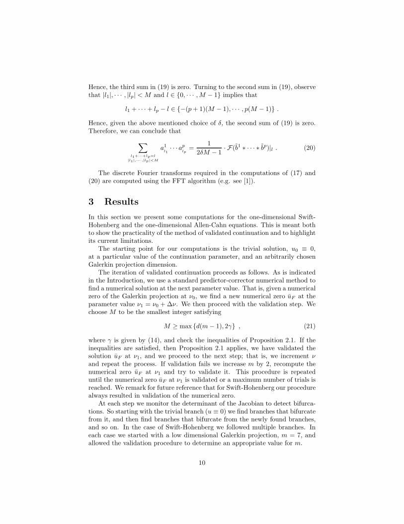
It is important to mention that we do not compute continuous branchesof equilibria. The symbols on Figures 1, 2, and 6, represent the points werewe computed and validated equilibrium solutions. Notice also that the stepsize from one step to the next is not constant, but changes along each branchaccording to the formula ∆ν := 2(4−k)/3∆ν, where k is the number of iterationsneeded for the Newton method during the continuation step [6].

0 1 2 3 4 5 60

0.5

1

1.5

2

2.5

ν

‖u‖

Figure 1: Bifurcation diagram for the Swift-Hohenberg equation (22) for 0 ≤ν ≤ 5. The symbols indicate the points at which a numerical zero was validated.

3.1 Swift-Hohenberg

Consider the Swift-Hohenberg equation [8]

ut =

(

ν −

(

1 +∂2

∂x2

)2)

u − u3, x ∈ [0, 2π/L] (22)

with u(x, t) = u(x+2π/L, t) and u(−x, t) = u(x, t). Expanding u in the Fourierbasis cos(kLx) | k = 0, 1, 2, . . . gives

u(x, t) = u0(t) + 2

∞∑

k=1

uk(t) cos(kLx).

11

Then (22) takes the form

uk = µkuk −∑

k1+k2+k3=k

uk1uk2uk3 ,

whereµk = ν −

(

1 − k2L2)2

, (23)

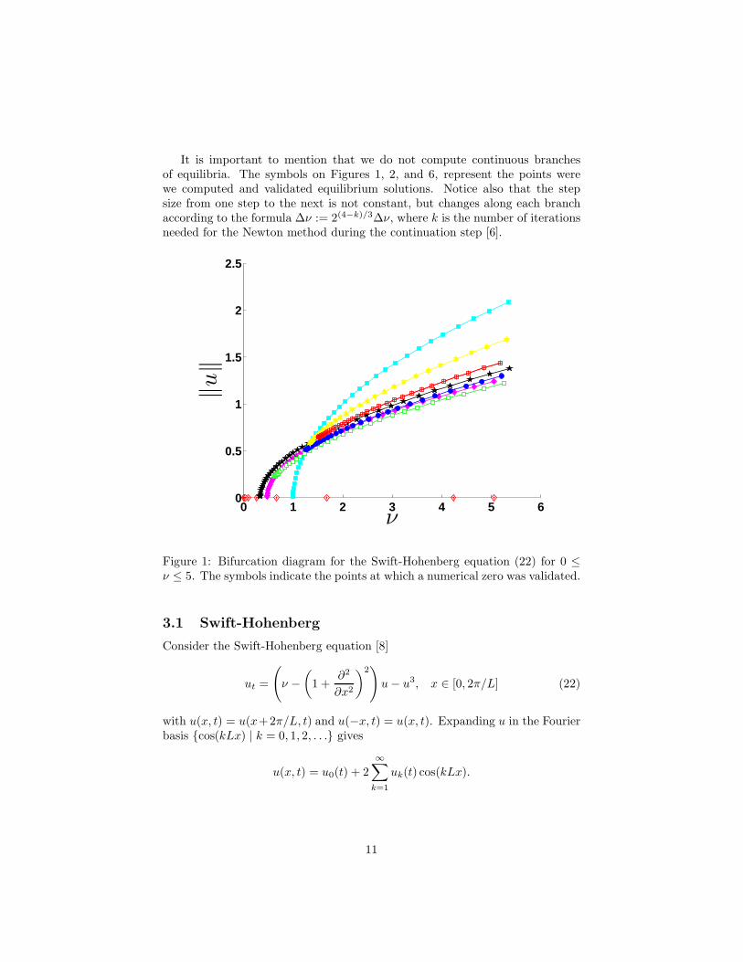
is the eigenvalue of the linear part of (22). We fix L = 0.65, and use ν as thecontinuation parameter.

0 2 4 6 8 10 12

x 105

0

200

400

600

800

1000

1200

ν

‖u‖

Figure 2: Some of the branches of equilibria of (22) for 0 ≤ ν ≤ 106. Thesymbols indicate the points at which a numerical zero was validated. For thevalues 0 ≤ ν ≤ 104 the validation was done using interval arithmetic and henceat these points we have a mathematical proof of the existence and uniquenessof these solutions in the sets Wu(r). The color coding and the symbols of thebranches in this figure matches that of Figure 1.

As is indicated in the Introduction, we view the set Wu(r), (5), as a functionof r. This implies that s and As are considered to be constants. For (22) we sets = 4 and As = 1. We discuss the choice of these values in Section 4.

We computed what we believe are all the branches of equilibria for 0 ≤ ν ≤ 5and followed some of the branches up to ν ≈ 106. The diagrams are shown onFigure 1 and Figure 2. We validated all the branches up to ν ≈ 104 in Figure 2using interval arithmetic to control floating point errors and thus rigorouslyverified that the inequalities of Proposition 2.1 are satisfied. This implies that

12

we have mathematically proven the existence and uniqueness within the setsWu(r) of the equilibria for Swift-Hohenberg at those values of ν ≤ 104 indicatedby the symbols in Figure 2.

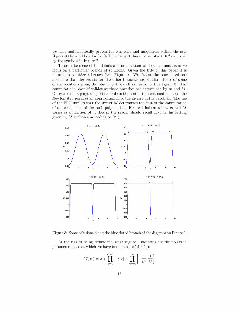
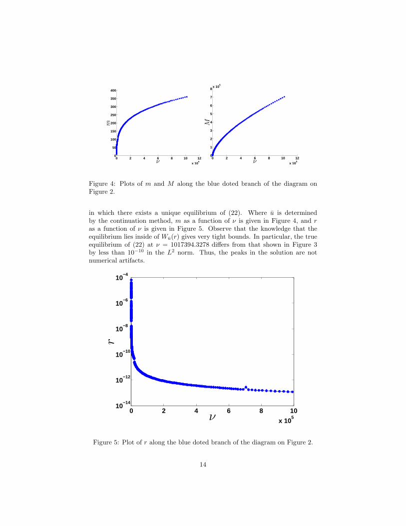
To describe some of the details and implications of these computations wefocus on a particular branch of solutions. Given the title of this paper it isnatural to consider a branch from Figure 2. We choose the blue doted oneand note that the results for the other branches are similar. Plots of someof the solutions along the blue doted branch are presented in Figure 3. Thecomputational cost of validating these branches are determined by m and M .Observe that m plays a significant role in the cost of the continuation step - theNewton step requires an approximation of the inverse of the Jacobian. The useof the FFT implies that the size of M determines the cost of the computationof the coefficients of the radii polynomials. Figure 4 indicates how m and Mvaries as a function of ν, though the reader should recall that in this settinggiven m, M is chosen according to (21).

0 2 4 6 8 100.49

0.5

0.51

0.52

0.53

0.54

x

u

ν = 1.2627

0 2 4 6 8 10−40

−20

0

20

40

60

80

x

u

ν = 4345.2728

0 2 4 6 8 10−200

−100

0

100

200

300

400

x

u

ν = 108301.2842

0 2 4 6 8 10−600

−400

−200

0

200

400

600

800

1000

1200

x

u

ν = 1017394.3278

Figure 3: Some solutions along the blue doted branch of the diagram on Figure 2.

At the risk of being redundant, what Figure 2 indicates are the points inparameter space at which we have found a set of the form

Wu(r) = u +

m−1∏

k=0

[−r, r] ×

∞∏

k=m

[

−1

k4,

1

k4

]

13

0 2 4 6 8 10 12

x 105

0

50

100

150

200

250

300

350

400

ν

m

0 2 4 6 8 10 12

x 105

0

1

2

3

4

5

6

7

8x 10

5

ν

M

Figure 4: Plots of m and M along the blue doted branch of the diagram onFigure 2.

in which there exists a unique equilibrium of (22). Where u is determinedby the continuation method, m as a function of ν is given in Figure 4, and ras a function of ν is given in Figure 5. Observe that the knowledge that theequilibrium lies inside of Wu(r) gives very tight bounds. In particular, the trueequilibrium of (22) at ν = 1017394.3278 differs from that shown in Figure 3by less than 10−10 in the L2 norm. Thus, the peaks in the solution are notnumerical artifacts.

0 2 4 6 8 10

x 105

10−14

10−12

10−10

10−8

10−6

10−4

ν

r

Figure 5: Plot of r along the blue doted branch of the diagram on Figure 2.

14

The computation time for the blue doted branch for ν up to ν ≈ 104 was6.5 minutes without interval arithmetic and 9.19 hours with interval arithmetic.The computation for the whole branch (up to ν ≈ 106) was 11.67 hours withoutinterval arithmetic. The computation times for the other branches were similar.The code is written in C++ and it was run on a Dual Core AMD Opteron 265(1.8GHz) with 3 GB of memory.

3.2 Allen-Cahn

We now turn our attention to the Allen-Cahn equation

ut = ǫ2uxx + u − u3, x ∈ Ω = [0, 1]ux = 0, on ∂Ω = 0, 1

(24)

For this equation we use λ = 1/ǫ2 as the continuation parameter. For (24)we use the Fourier basis cos(kπx) | k = 0, 1, 2, . . ., then

u(x, t) = u0(t) + 2

∞∑

k=1

uk(t) cos(kπx).

So (24) takes the form

uk = µkuk −∑

k1+k2+k3=k

uk1uk2uk3 ,

where

µk = 1 −k2π2

λ(25)

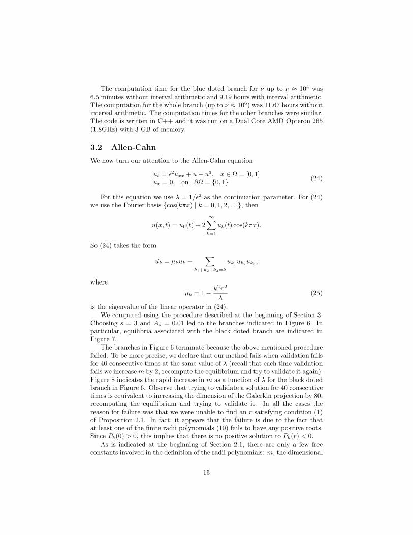
is the eigenvalue of the linear operator in (24).We computed using the procedure described at the beginning of Section 3.

Choosing s = 3 and As = 0.01 led to the branches indicated in Figure 6. Inparticular, equilibria associated with the black doted branch are indicated inFigure 7.

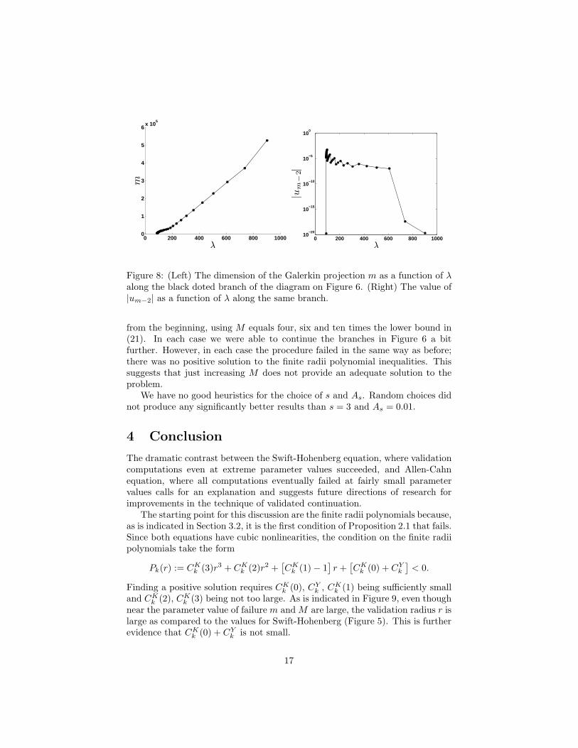
The branches in Figure 6 terminate because the above mentioned procedurefailed. To be more precise, we declare that our method fails when validation failsfor 40 consecutive times at the same value of λ (recall that each time validationfails we increase m by 2, recompute the equilibrium and try to validate it again).Figure 8 indicates the rapid increase in m as a function of λ for the black dotedbranch in Figure 6. Observe that trying to validate a solution for 40 consecutivetimes is equivalent to increasing the dimension of the Galerkin projection by 80,recomputing the equilibrium and trying to validate it. In all the cases thereason for failure was that we were unable to find an r satisfying condition (1)of Proposition 2.1. In fact, it appears that the failure is due to the fact thatat least one of the finite radii polynomials (10) fails to have any positive roots.Since Pk(0) > 0, this implies that there is no positive solution to Pk(r) < 0.

As is indicated at the beginning of Section 2.1, there are only a few freeconstants involved in the definition of the radii polynomials: m, the dimensional

15

0 200 400 600 800 10000

0.1

0.2

0.3

0.4

0.5

0.6

0.7

λ

‖u‖

Figure 6: The computed branches of equilibria for (24).

0 0.2 0.4 0.6 0.8 1−0.1

−0.05

0

0.05

0.1

x

u

λ = 89.4977

0 0.2 0.4 0.6 0.8 1−1

−0.5

0

0.5

1

x

u

λ = 902.0465

Figure 7: Solutions along the black doted branch of the diagram on Figure 6.

of the Galerkin projection; M , a computational parameter; s, the decay rate;and As an a priori bound on the size of the Fourier coefficients. As is describedabove, failure of the procedure implies that m has been increased by 80. As onemay expect and as the results in Figure 8 corroborates, this implies values ofuk for k close to m are essentially zero. Thus, further increase of the Galerkinprojection at this point has little effect on the validation procedure.

We tried to increase the value of M , since this results in better control on thetail errors. In particular, all the results indicated in Figure 6 were obtained usingM equals twice the lower bound given by (21). We tried the same computations,

16

0 200 400 600 800 10000

1

2

3

4

5

6x 10

5

λ

m

0 200 400 600 800 100010

−20

10−15

10−10

10−5

100

λ

|um

−2|

Figure 8: (Left) The dimension of the Galerkin projection m as a function of λalong the black doted branch of the diagram on Figure 6. (Right) The value of|um−2| as a function of λ along the same branch.

from the beginning, using M equals four, six and ten times the lower bound in(21). In each case we were able to continue the branches in Figure 6 a bitfurther. However, in each case the procedure failed in the same way as before;there was no positive solution to the finite radii polynomial inequalities. Thissuggests that just increasing M does not provide an adequate solution to theproblem.

We have no good heuristics for the choice of s and As. Random choices didnot produce any significantly better results than s = 3 and As = 0.01.

4 Conclusion

The dramatic contrast between the Swift-Hohenberg equation, where validationcomputations even at extreme parameter values succeeded, and Allen-Cahnequation, where all computations eventually failed at fairly small parametervalues calls for an explanation and suggests future directions of research forimprovements in the technique of validated continuation.

The starting point for this discussion are the finite radii polynomials because,as is indicated in Section 3.2, it is the first condition of Proposition 2.1 that fails.Since both equations have cubic nonlinearities, the condition on the finite radiipolynomials take the form

Pk(r) := CKk (3)r3 + CK

k (2)r2 +[

CKk (1) − 1

]

r +[

CKk (0) + CY

k

]

< 0.

Finding a positive solution requires CKk (0), CY

k , CKk (1) being sufficiently small

and CKk (2), CK

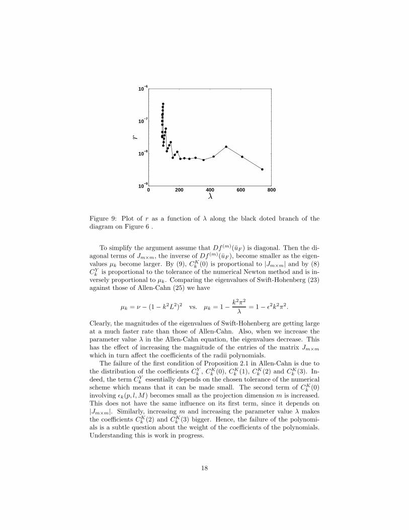
k (3) being not too large. As is indicated in Figure 9, even thoughnear the parameter value of failure m and M are large, the validation radius r islarge as compared to the values for Swift-Hohenberg (Figure 5). This is furtherevidence that CK

k (0) + CYk is not small.

17

0 200 400 600 80010

−9

10−8

10−7

10−6

λ

r

Figure 9: Plot of r as a function of λ along the black doted branch of thediagram on Figure 6 .

To simplify the argument assume that Df (m)(uF ) is diagonal. Then the di-agonal terms of Jm×m, the inverse of Df (m)(uF ), become smaller as the eigen-values µk become larger. By (9), CK

k (0) is proportional to |Jm×m| and by (8)CY

k is proportional to the tolerance of the numerical Newton method and is in-versely proportional to µk. Comparing the eigenvalues of Swift-Hohenberg (23)against those of Allen-Cahn (25) we have

µk = ν − (1 − k2L2)2 vs. µk = 1 −k2π2

λ= 1 − ǫ2k2π2.

Clearly, the magnitudes of the eigenvalues of Swift-Hohenberg are getting largeat a much faster rate than those of Allen-Cahn. Also, when we increase theparameter value λ in the Allen-Cahn equation, the eigenvalues decrease. Thishas the effect of increasing the magnitude of the entries of the matrix Jm×m

which in turn affect the coefficients of the radii polynomials.The failure of the first condition of Proposition 2.1 in Allen-Cahn is due to

the distribution of the coefficients CYk , CK

k (0), CKk (1), CK

k (2) and CKk (3). In-

deed, the term CYk essentially depends on the chosen tolerance of the numerical

scheme which means that it can be made small. The second term of CKk (0)

involving ǫk(p, l, M) becomes small as the projection dimension m is increased.This does not have the same influence on its first term, since it depends on|Jm×m|. Similarly, increasing m and increasing the parameter value λ makesthe coefficients CK

k (2) and CKk (3) bigger. Hence, the failure of the polynomi-

als is a subtle question about the weight of the coefficients of the polynomials.Understanding this is work in progress.

18

References

[1] E. Brigham, Fast Fourier Transform and its Applications, Prentice Hall,1st edition, (1988).

[2] J. W. Cahn and J. E. Hilliard, Free energy of a nonuniform system I.Interfacial free energy, Journal of Chemical Physics, 28, pp. 258–267, (1958).

[3] S. Day, Y. Hiraoka, K. Mischaikow, and T. Ogawa, Rigorous nu-merics for global dynamics: A study of the Swift-Hohenberg equation, SIAMJournal on Applied Dynamical Systems, 4, pp. 1–31, (2005).

[4] S. Day, J.-P. Lessard, and K. Mischaikow, Validated Continuationfor Equilibria of PDEs, SIAM Journal on Numerical Analysis, 45 (4), pp.1398-1424, (2007).

[5] Y. Hiraoka, and T. Ogawa, An efficient estimate based on FFT in topo-logical verification method, J. Comput. Appl. Math. 199, no. 2, pp. 238–244,(2007).

[6] H. B. Keller, Lectures on numerical methods in bifurcation problems, TataInstitute of Fundamental Research Lectures on Mathematics and Physics,79, Springer-Verlag, Berlin, (1987).

[7] J.-P. Lessard, Validated Continuation for Infinite Dimensional Problems,Ph.D Thesis, Georgia Institute of Technology, (2007).

[8] J. B. Swift and P. C. Hohenberg, Hydrodynamic fluctuations at theconvective instability, Physical Review A, 15:319, (1977).

[9] N. Yamamoto, A numerical verification method for solutions of boundaryvalue problems with local uniqueness by Banach’s fixed-point theorem, SIAMJournal on Numerical Analysis, 35, pp. 2004–2013, (1998).

[10] P. Zgliczynski and K. Mischaikow, Rigorous numerics for partialdifferential equations: The Kuramoto-Sivashinsky equation, Foundations ofComputational Mathematics, 1, pp. 255–288, (2001).

19