Two-way ANOVA - UCSD Cognitive Sciencenunez/COGS14B_W17/W9.pdf · One-way χ2 test One-way χ2 test...
6
1 Two-way ANOVA ! Calculations Two-way ANOVA ! Calculations Two-way ANOVA ! Final Table F table (critical values) ! Non-parametric statistics ! A test for qualitative (categorical) data ! One-way Chi-square (χ 2 ) ! Two-way Chi-square (χ 2 ) II. Inferential Statistics (13) 1.- Non-parametric statistics ! Designed for cases when … ! no population parameters (e.g., μ, σ, ρ, etc) ! measurement is done with nominal or ordinal scales (qualitative) ! Also called distribution-free tests
Transcript of Two-way ANOVA - UCSD Cognitive Sciencenunez/COGS14B_W17/W9.pdf · One-way χ2 test One-way χ2 test...

1
Two-way ANOVA ! Calculations
Two-way ANOVA ! Calculations
Two-way ANOVA ! Final Table
F table (critical values)
! Non-parametric statistics ! A test for qualitative (categorical) data
! One-way Chi-square (χ2) ! Two-way Chi-square (χ2)
II. Inferential Statistics (13) 1.- Non-parametric statistics
! Designed for cases when … ! no population parameters (e.g., µ, σ, ρ, etc) ! measurement is done with nominal or ordinal
scales (qualitative) ! Also called distribution-free tests

2
2. A test for categorical data ! Chi-square χ2 ! Used when observations are merely classified
into various categories
One-way χ2 test ! Evaluates whether observed frequencies for a single
qualitative variable are adequately described by hypothesized or expected frequencies
! Goodness-of-fit test ! Statistical Hypotheses:
! H0: P1=p1; P2=p2; … Pk=pk (p1+p2+…pk= 1)
! H1: H0 is false
One-way χ2 test ! How old is she?
Young: 54.3% Old: 45.7%
Priming experiment
One-way χ2 test ! Example:
Old Young Total
Observed frequency (fo)
42 25 67
Expected frequency (fe)
30.62 (45.7%)
36.38 (54.3%)
67 (100%)
H0: POld = .457; PYoung =.543 H1: H0 is false
One-way χ2 test ! Expected frequency (fe)
! The hypothesized frequency for each category, given that the null hypothesis is true.
! fe = (expected proportion)(total sample size)
! Observed frequency (fo) ! The obtained frequency for each category
3
One-way χ2 test ! Calculation of χ2
! The larger the discrepancies between fo and fe, the larger the value of χ2 (more suspect H0 will be)
! χ2 is always positive (test is non-directional) ! Division by fe indicates that discrepancies are not
evaluated in absolute terms but relative to the size of expected frequencies.
χ2 = Σ (fo – fe)2
fe
One-way χ2 test ! Example:
Old Young Total
Observed frequency (fo)
42 25 67
Expected frequency (fe)
30.62 (45.7%)
36.38 (54.3%)
67 (100%)
χ2 = [(42-30.62)2]/30.62 + [(25-36.38)2]/36.38
χ2 = 4.23 + 3.56 = 7.79
χ2 = 7.79** df = C-1 = 1
One-way χ2 test One-way χ2 test ! In our experiment …
! χ2 = 7.79 is bigger than 6.63 (cv at .01 level of significance with 1 df)
! Therefore we reject H0. ! Interepretation: The proportions of responses Old-
Young after priming differ from the proportions reported in the specialized litterature
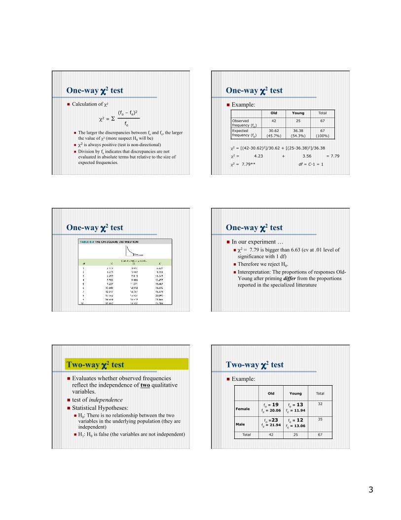
Two-way χ2 test ! Evaluates whether observed frequencies
reflect the independence of two qualitative variables.
! test of independence ! Statistical Hypotheses:
! H0: There is no relationship between the two variables in the underlying population (they are independent)
! H1: H0 is false (the variables are not independent)
Two-way χ2 test ! Example:
Old Young Total
Female fo = 19
fe = 20.06 fo = 13
fe = 11.94
32
Male fo =23
fe = 21.94 fo = 12
fe = 13.06
35
Total 42 25 67
4
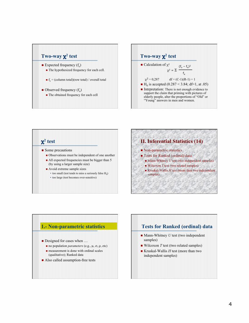
Two-way χ2 test ! Expected frequency (fe)
! The hypothesized frequency for each cell.
! fe = (column total)(row total) / overall total
! Observed frequency (fo) ! The obtained frequency for each cell
Two-way χ2 test ! Calculation of χ2
χ2 = 0,287 df = (C-1)(R-1) = 1 ! H0 is accepted (0.287 < 3.84; df=1, at .05) ! Intrpretation: There is not enough evidence to
support the claim that priming with pictures of elderly people, alter the proportions of “Old” or “Young” answers in men and women.
χ2 = Σ (fo – fe)2
fe
χ2 test ! Some precautions
! Observations must be independent of one another ! All expected frequencies must be bigger than 5
(by using a larger sample size) ! Avoid extreme sample sizes
• too small (test tends to miss a seriously false H0) • too large (test becomes over-sensitive)
! Non-parametric statistics ! Tests for Ranked (ordinal) data
! Mann-Whitney U test (two independent samples) ! Wilcoxon T test (two related samples) ! Kruskal-Wallis H test (more than two independent
samples)
II. Inferential Statistics (14)
1.- Non-parametric statistics
! Designed for cases when … ! no population parameters (e.g., µ, σ, ρ, etc) ! measurement is done with ordinal scales
(qualitative); Ranked data ! Also called assumption-free tests
Tests for Ranked (ordinal) data ! Mann-Whitney U test (two independent
samples) ! Wilcoxon T test (two related samples) ! Kruskal-Wallis H test (more than two
independent samples)
5
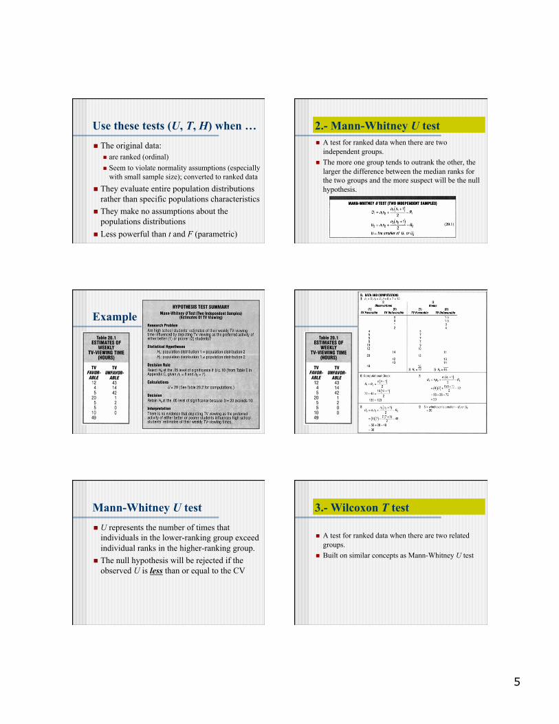
Use these tests (U, T, H) when … ! The original data:
! are ranked (ordinal) ! Seem to violate normality assumptions (especially
with small sample size); converted to ranked data ! They evaluate entire population distributions
rather than specific populations characteristics ! They make no assumptions about the
populations distributions ! Less powerful than t and F (parametric)
2.- Mann-Whitney U test ! A test for ranked data when there are two
independent groups. ! The more one group tends to outrank the other, the
larger the difference between the median ranks for the two groups and the more suspect will be the null hypothesis.
Example
Mann-Whitney U test ! U represents the number of times that
individuals in the lower-ranking group exceed individual ranks in the higher-ranking group.
! The null hypothesis will be rejected if the observed U is less than or equal to the CV
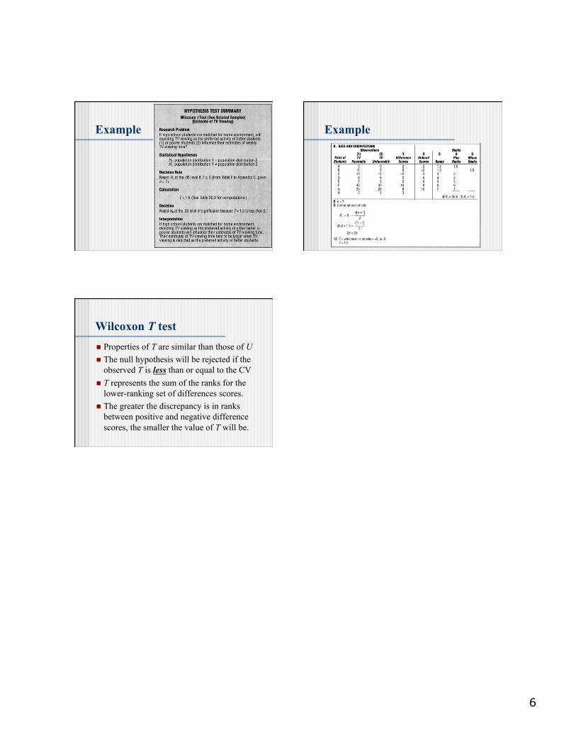
3.- Wilcoxon T test
! A test for ranked data when there are two related groups.
! Built on similar concepts as Mann-Whitney U test
6
Example Example
Wilcoxon T test ! Properties of T are similar than those of U ! The null hypothesis will be rejected if the
observed T is less than or equal to the CV ! T represents the sum of the ranks for the
lower-ranking set of differences scores. ! The greater the discrepancy is in ranks
between positive and negative difference scores, the smaller the value of T will be.