Two-loop corrections to the Higgs trilinear coupling in models with

classical scale invariance

Johannes Braathen (DESY)Based on arXiv:2011.07580

with Shinya Kanemura and Makoto Shimoda (Osaka U.)

November 19, 2020

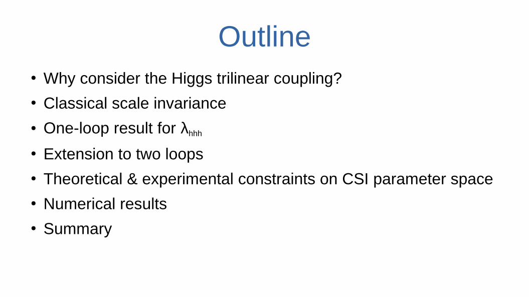
Outline● Why consider the Higgs trilinear coupling?● Classical scale invariance● One-loop result for λhhh

● Extension to two loops● Theoretical & experimental constraints on CSI parameter space● Numerical results● Summary

Introduction/Motivation

Why investigate λhhh

? 1/2

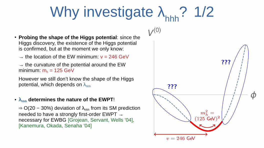
● Probing the shape of the Higgs potential: since the Higgs discovery, the existence of the Higgs potential is confirmed, but at the moment we only know:

→ the location of the EW minimum: v = 246 GeV

→ the curvature of the potential around the EW minimum: mh = 125 GeV

However we still don’t know the shape of the Higgs potential, which depends on λhhh

● λhhh determines the nature of the EWPT!

⇒ O(20 − 30%) deviation of λhhh from its SM prediction needed to have a strongly first-order EWPT → necessary for EWBG [Grojean, Servant, Wells ’04], [Kanemura, Okada, Senaha ’04]

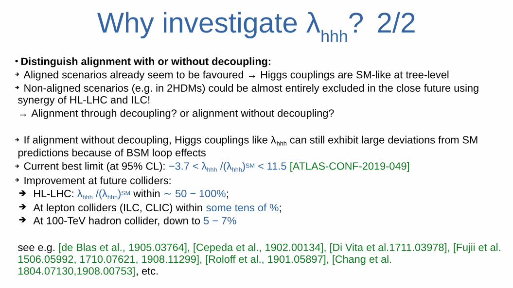
Why investigate λhhh

? 2/2● Distinguish alignment with or without decoupling:➔ Aligned scenarios already seem to be favoured → Higgs couplings are SM-like at tree-level➔ Non-aligned scenarios (e.g. in 2HDMs) could be almost entirely excluded in the close future using synergy of HL-LHC and ILC!→ Alignment through decoupling? or alignment without decoupling?

➔ If alignment without decoupling, Higgs couplings like λhhh can still exhibit large deviations from SM predictions because of BSM loop effects

➔ Current best limit (at 95% CL): −3.7 < λhhh /(λhhh)SM < 11.5 [ATLAS-CONF-2019-049]➔ Improvement at future colliders: ➔ HL-LHC: λhhh /(λhhh)SM within 50 − 100%∼ ; ➔ At lepton colliders (ILC, CLIC) within some tens of %; ➔ At 100-TeV hadron collider, down to 5 − 7%

see e.g. [de Blas et al., 1905.03764], [Cepeda et al., 1902.00134], [Di Vita et al.1711.03978], [Fujii et al. 1506.05992, 1710.07621, 1908.11299], [Roloff et al., 1901.05897], [Chang et al. 1804.07130,1908.00753], etc.

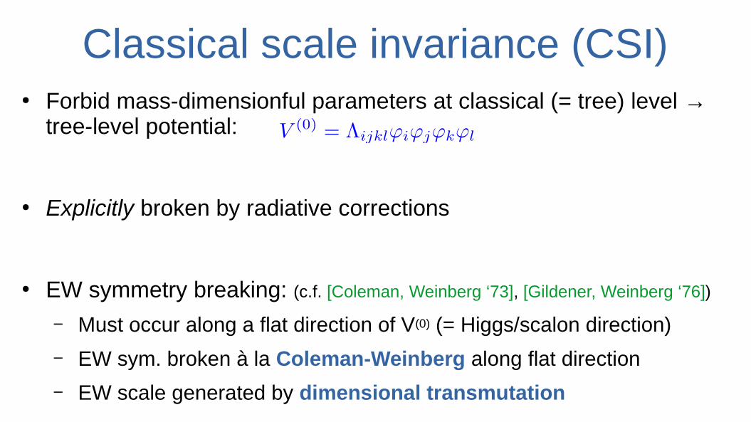
Classical scale invariance (CSI)● Forbid mass-dimensionful parameters at classical (= tree) level →

tree-level potential:

● Explicitly broken by radiative corrections

● EW symmetry breaking: (c.f. [Coleman, Weinberg ‘73], [Gildener, Weinberg ‘76])

– Must occur along a flat direction of V(0) (= Higgs/scalon direction)

– EW sym. broken à la Coleman-Weinberg along flat direction

– EW scale generated by dimensional transmutation

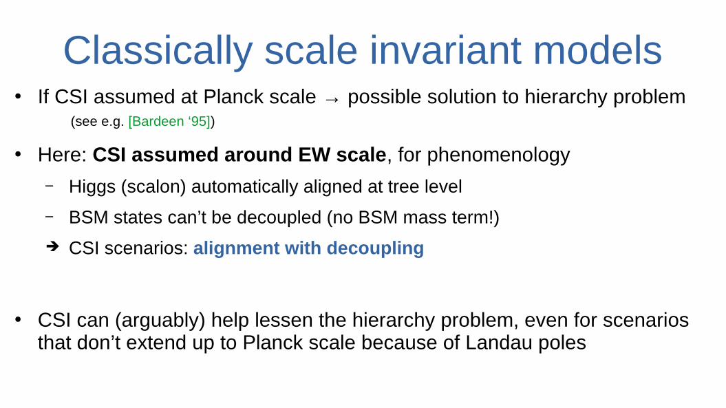
Classically scale invariant models● If CSI assumed at Planck scale → possible solution to hierarchy problem

(see e.g. [Bardeen ‘95])

● Here: CSI assumed around EW scale, for phenomenology

– Higgs (scalon) automatically aligned at tree level

– BSM states can’t be decoupled (no BSM mass term!)

➔ CSI scenarios: alignment with decoupling

● CSI can (arguably) help lessen the hierarchy problem, even for scenarios that don’t extend up to Planck scale because of Landau poles

Calculational setup

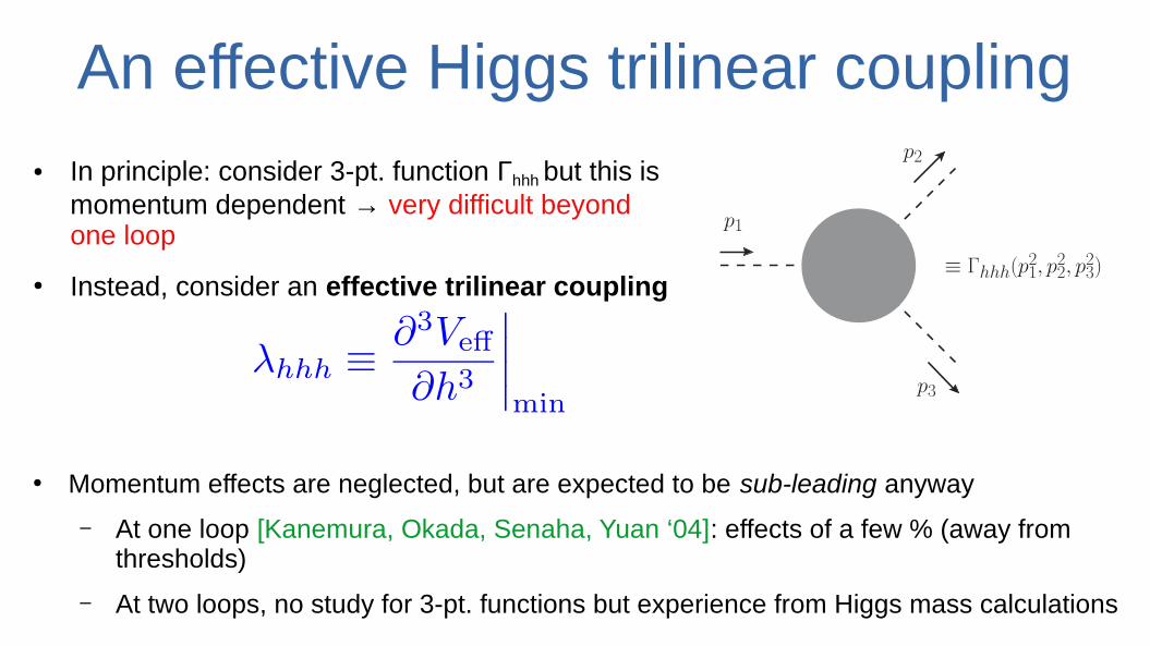
An effective Higgs trilinear coupling● In principle: consider 3-pt. function Γhhh but this is

momentum dependent → very difficult beyond one loop

● Instead, consider an effective trilinear coupling

p1

p2

p3

≡ Γhhh(p21, p

22, p

23)

● Momentum effects are neglected, but are expected to be sub-leading anyway

– At one loop [Kanemura, Okada, Senaha, Yuan ‘04]: effects of a few % (away from thresholds)

– At two loops, no study for 3-pt. functions but experience from Higgs mass calculations

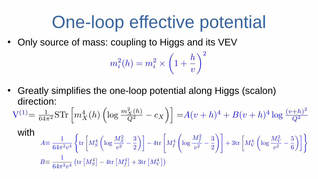
One-loop effective potential● Only source of mass: coupling to Higgs and its VEV

● Greatly simplifies the one-loop potential along Higgs (scalon) direction:

with

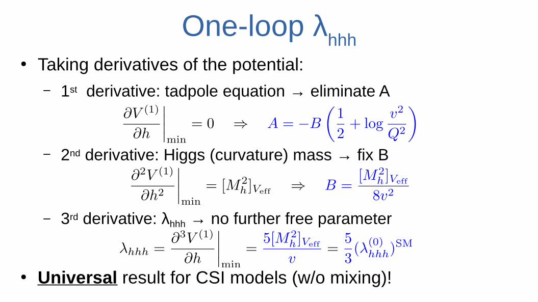
One-loop λhhh

● Taking derivatives of the potential:– 1st derivative: tadpole equation → eliminate A

– 2nd derivative: Higgs (curvature) mass → fix B

– 3rd derivative: λhhh → no further free parameter

● Universal result for CSI models (w/o mixing)!

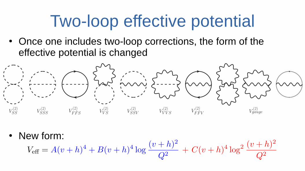
Two-loop effective potential● Once one includes two-loop corrections, the form of the

effective potential is changed

● New form:

V(2)SS V

(2)SSS V

(2)FF̄S V

(2)V S V

(2)SSV V

(2)V V S V

(2)FF̄V V

(2)gauge

.

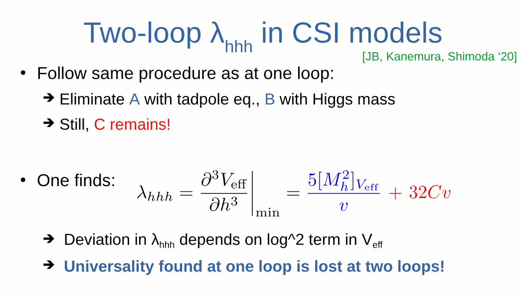
Two-loop λhhh

in CSI models● Follow same procedure as at one loop:

➔ Eliminate A with tadpole eq., B with Higgs mass

➔ Still, C remains!

● One finds:

➔ Deviation in λhhh depends on log^2 term in Veff

➔ Universality found at one loop is lost at two loops!

[JB, Kanemura, Shimoda ‘20]

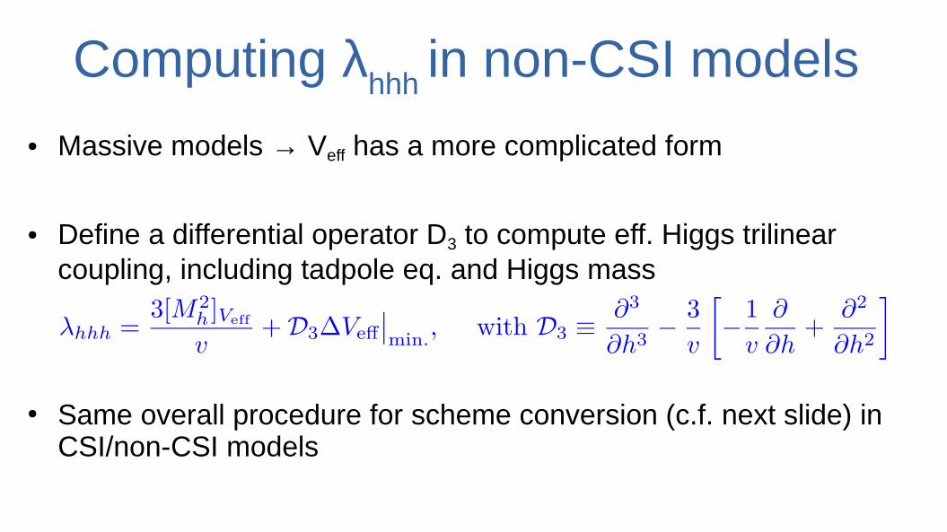
Computing λhhh

in non-CSI models ● Massive models → Veff has a more complicated form

● Define a differential operator D3 to compute eff. Higgs trilinear coupling, including tadpole eq. and Higgs mass

● Same overall procedure for scheme conversion (c.f. next slide) in CSI/non-CSI models

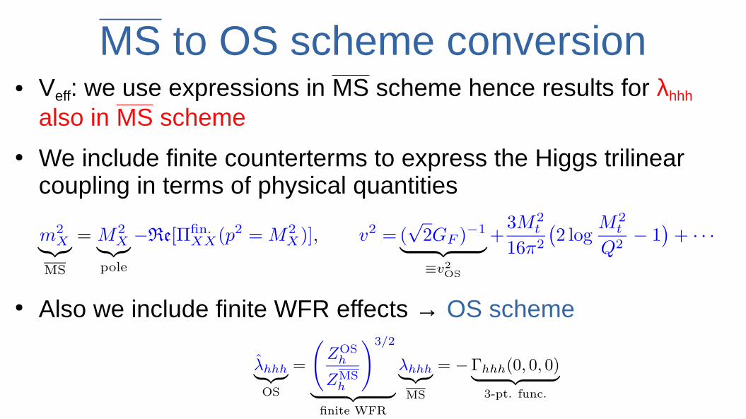
MS to OS scheme conversion● Veff: we use expressions in MS scheme hence results for λhhh

also in MS scheme

● We include finite counterterms to express the Higgs trilinear coupling in terms of physical quantities

● Also we include finite WFR effects → OS scheme

Numerical analysis

Our questions:- how large can two-loop effects be?

- can they allow distinguishing CSI vs non-CSI?

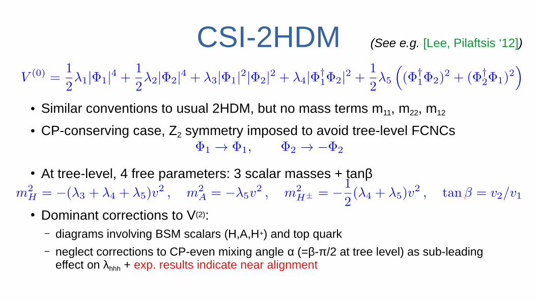
CSI-2HDM

● Similar conventions to usual 2HDM, but no mass terms m11, m22, m12

● CP-conserving case, Z2 symmetry imposed to avoid tree-level FCNCs

● At tree-level, 4 free parameters: 3 scalar masses + tanβ

● Dominant corrections to V(2): – diagrams involving BSM scalars (H,A,H+) and top quark– neglect corrections to CP-even mixing angle α (=β-π/2 at tree level) as sub-leading

effect on λhhh + exp. results indicate near alignment

(See e.g. [Lee, Pilaftsis ‘12])

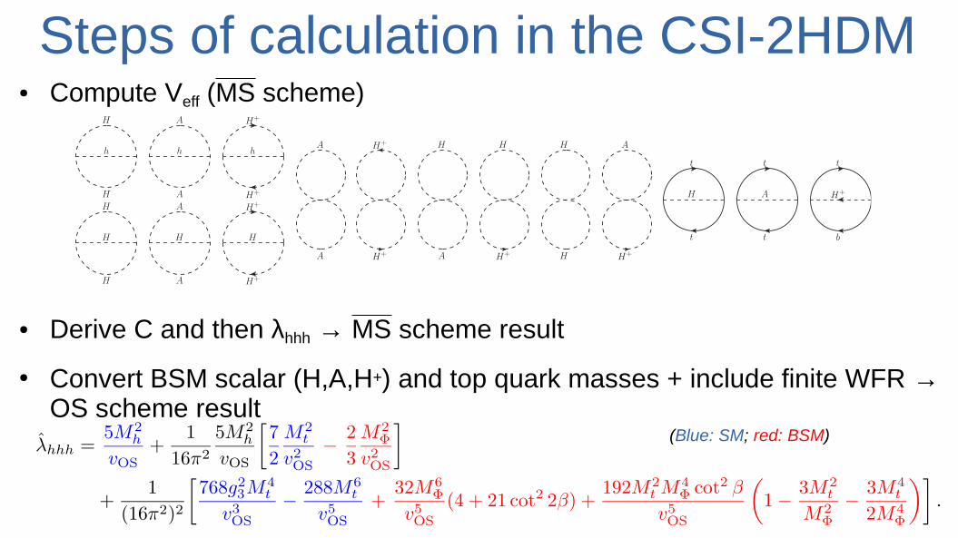
Steps of calculation in the CSI-2HDM● Compute Veff (MS scheme)

● Derive C and then λhhh → MS scheme result

● Convert BSM scalar (H,A,H+) and top quark masses + include finite WFR → OS scheme result

.

H

H

A

A

H+

H+

A

H H

H+

A

H+

H+

b

t

H

t

t

t

t

A

A

A

H+

H+

H

H

H

H

A

A

H+

H+

h

H H H

h h

(Blue: SM; red: BSM)

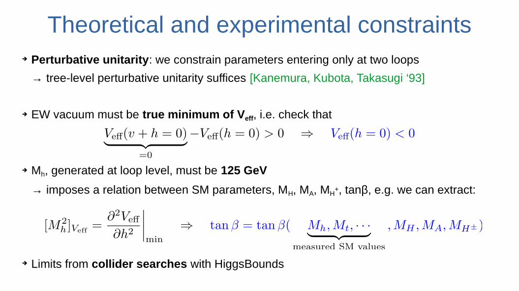
Theoretical and experimental constraints➔ Perturbative unitarity: we constrain parameters entering only at two loops

→ tree-level perturbative unitarity suffices [Kanemura, Kubota, Takasugi ‘93]

➔ EW vacuum must be true minimum of Veff, i.e. check that

➔ Mh, generated at loop level, must be 125 GeV

→ imposes a relation between SM parameters, MH, MA, MH+, tanβ, e.g. we can extract:

➔ Limits from collider searches with HiggsBounds

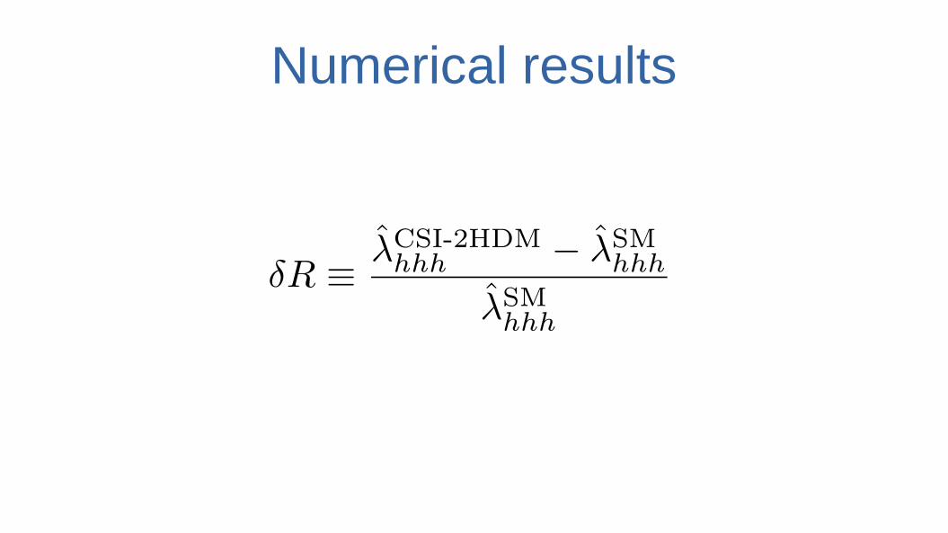
Numerical results

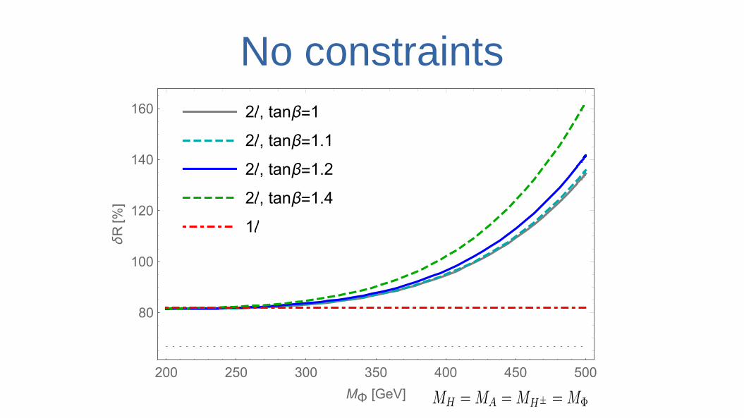
No constraints2ℓ, tanβ=1

2ℓ, tanβ=1.1

2ℓ, tanβ=1.2

2ℓ, tanβ=1.4

1ℓ

200 250 300 350 400 450 500

80

100

120

140

160

MΦ [GeV]

δR[%

]

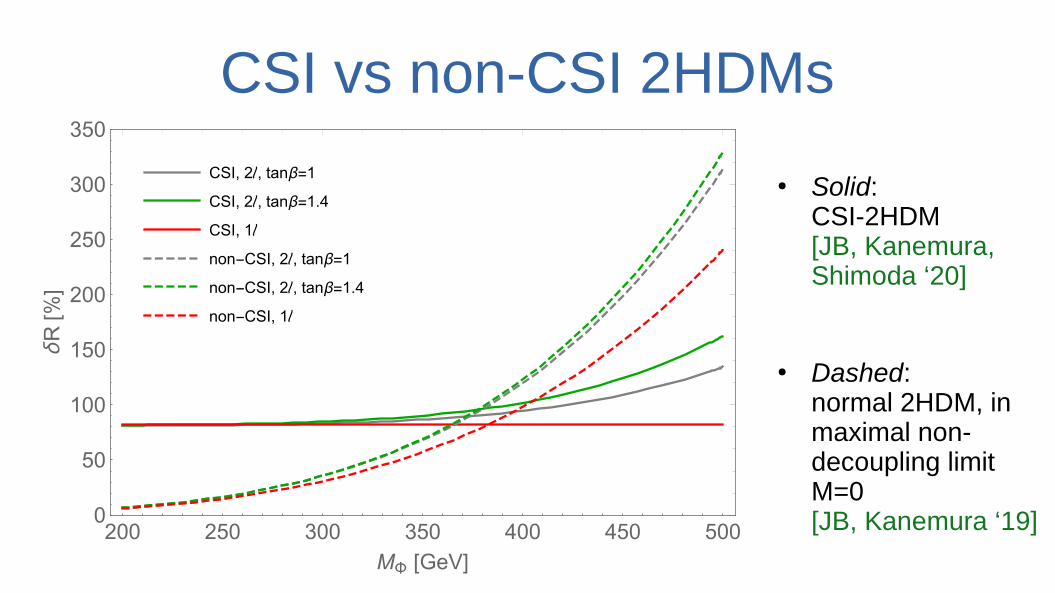
CSI vs non-CSI 2HDMs

CSI, 2ℓ, tanβ=1

CSI, 2ℓ, tanβ=1.4

CSI, 1ℓ

non-CSI, 2ℓ, tanβ=1

non-CSI, 2ℓ, tanβ=1.4

non-CSI, 1ℓ

200 250 300 350 400 450 5000

50

100

150

200

250

300

350

MΦ [GeV]

δR[%

]

● Solid: CSI-2HDM [JB, Kanemura, Shimoda ‘20]

● Dashed: normal 2HDM, in maximal non-decoupling limit M=0 [JB, Kanemura ‘19]

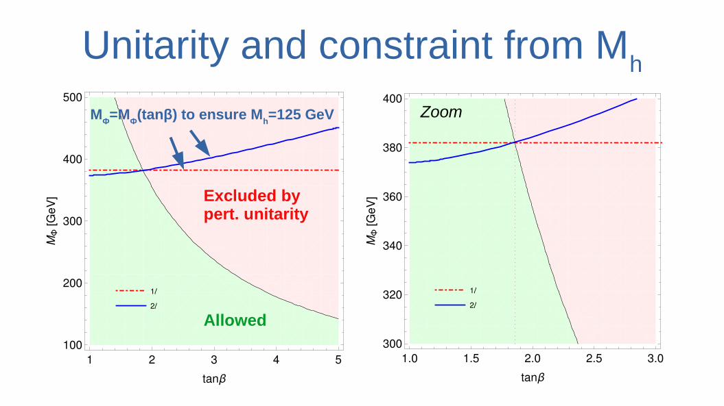
Unitarity and constraint from Mh

1ℓ

2ℓ

1 2 3 4 5

100

200

300

400

500

tanβ

MΦ[G

eV]

1ℓ

2ℓ

1.0 1.5 2.0 2.5 3.0

300

320

340

360

380

400

tanβM

Φ[G

eV]Excluded by pert. unitarity

Allowed

MΦ=M

Φ(tanβ) to ensure M

h=125 GeV Zoom

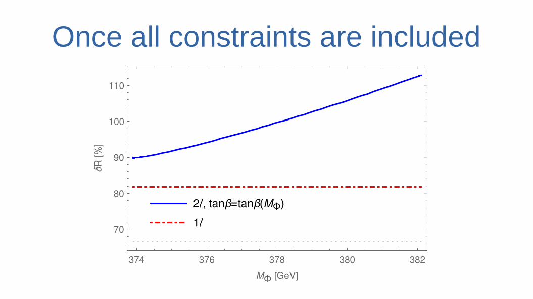
Once all constraints are included

2ℓ, tanβ=tanβ(MΦ)

1ℓ

374 376 378 380 382

70

80

90

100

110

MΦ [GeV]

δR

[%]

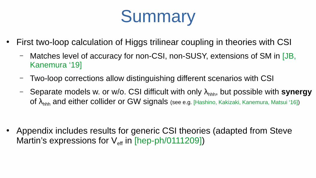
Summary● First two-loop calculation of Higgs trilinear coupling in theories with CSI

– Matches level of accuracy for non-CSI, non-SUSY, extensions of SM in [JB, Kanemura ‘19]

– Two-loop corrections allow distinguishing different scenarios with CSI

– Separate models w. or w/o. CSI difficult with only λhhh, but possible with synergy of λhhh and either collider or GW signals (see e.g. [Hashino, Kakizaki, Kanemura, Matsui ‘16])

● Appendix includes results for generic CSI theories (adapted from Steve Martin’s expressions for Veff in [hep-ph/0111209])

Thank you very much for your attention!