8– NMR Interactions: Dipolar Coupling 8.1 Hamiltoniangroups.chem.ubc.ca/straus/l4.pdf · 8.14 are...
18
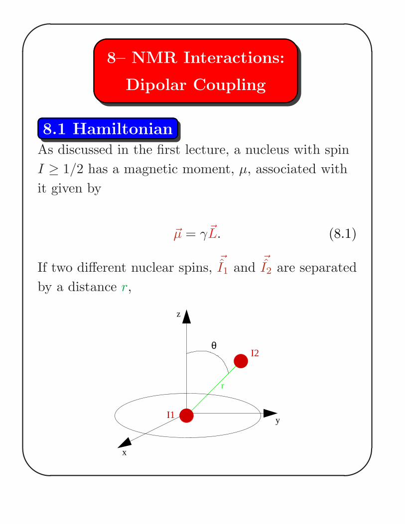
✬ ✫ ✩ ✪ 8– NMR Interactions: Dipolar Coupling 8.1 Hamiltonian As discussed in the first lecture, a nucleus with spin I ≥ 1/2 has a magnetic moment, μ, associated with it given by μ = γ L. (8.1) If two different nuclear spins, ˆ I 1 and ˆ I 2 are separated by a distance r , z I1 I2 x y θ r
Transcript of 8– NMR Interactions: Dipolar Coupling 8.1 Hamiltoniangroups.chem.ubc.ca/straus/l4.pdf · 8.14 are...
'
&
$
%
8– NMR Interactions:
Dipolar Coupling
8.1 Hamiltonian
As discussed in the first lecture, a nucleus with spin
I ≥ 1/2 has a magnetic moment, µ, associated with
it given by
~µ = γ~L. (8.1)
If two different nuclear spins,~I1 and
~I2 are separated
by a distance r,
z
I1
I2
x
y
θ
r
'
&
$
%
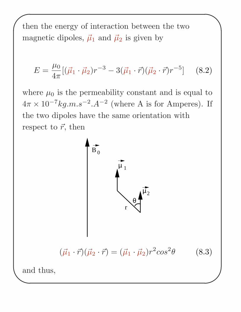
then the energy of interaction between the two
magnetic dipoles, ~µ1 and ~µ2 is given by
E =µ0
4π[(~µ1 · ~µ2)r
−3 − 3(~µ1 · ~r)(~µ2 · ~r)r−5] (8.2)
where µ0 is the permeability constant and is equal to
4π × 10−7kg.m.s−2.A−2 (where A is for Amperes). If
the two dipoles have the same orientation with
respect to ~r, then
rθ
µ
B 0
1
µ2
(~µ1 · ~r)(~µ2 · ~r) = (~µ1 · ~µ2)r2cos2θ (8.3)
and thus,
'
&
$
%
E =µ0
4π(~µ1 · ~µ2)r
−3[1 − 3cos2θ]. (8.4)
where ~µ1 · ~µ2 = µ1µ2 since they are parallel.
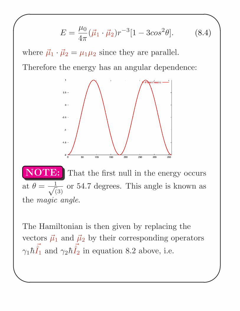
Therefore the energy has an angular dependence:
NOTE: That the first null in the energy occurs
at θ = 1√(3)
or 54.7 degrees. This angle is known as
the magic angle.
The Hamiltonian is then given by replacing the
vectors ~µ1 and ~µ2 by their corresponding operators
γ1h~I1 and γ2h
~I2 in equation 8.2 above, i.e.
'
&
$
%
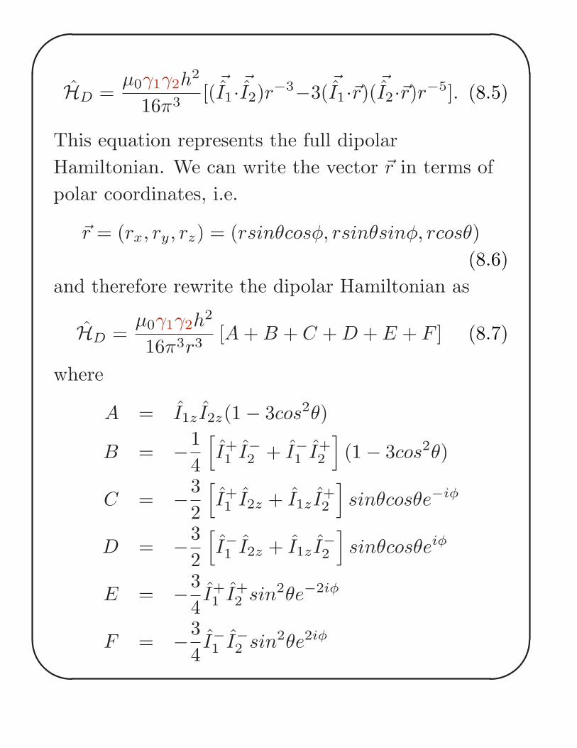
HD =µ0γ1γ2h
2
16π3[(
~I1· ~I2)r
−3−3(~I1·~r)( ~
I2·~r)r−5]. (8.5)
This equation represents the full dipolar
Hamiltonian. We can write the vector ~r in terms of
polar coordinates, i.e.
~r = (rx, ry, rz) = (rsinθcosφ, rsinθsinφ, rcosθ)
(8.6)
and therefore rewrite the dipolar Hamiltonian as
HD =µ0γ1γ2h
2
16π3r3[A + B + C + D + E + F ] (8.7)
where
A = I1z I2z(1 − 3cos2θ)
B = −1
4
[
I+1 I−2 + I−1 I+
2
]
(1 − 3cos2θ)
C = −3
2
[
I+1 I2z + I1z I
+2
]
sinθcosθe−iφ
D = −3
2
[
I−1 I2z + I1z I−2
]
sinθcosθeiφ
E = −3
4I+1 I+
2 sin2θe−2iφ
F = −3
4I−1 I−2 sin2θe2iφ
'
&
$
%
(8.8)
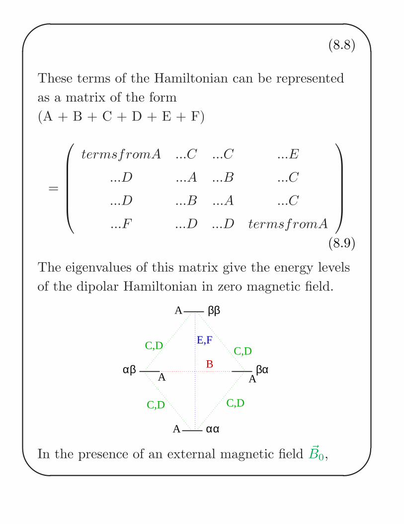
These terms of the Hamiltonian can be represented
as a matrix of the form
(A + B + C + D + E + F)
=
termsfromA ...C ...C ...E
...D ...A ...B ...C
...D ...B ...A ...C
...F ...D ...D termsfromA
(8.9)
The eigenvalues of this matrix give the energy levels
of the dipolar Hamiltonian in zero magnetic field.
αα
αβ βαB
E,F
ββ
C,D
C,DC,D
C,D
A
A
AA
In the presence of an external magnetic field ~B0,
'
&
$
%
however, many of the higher order terms can be
neglected, i.e. if the following condition is valid:
|ω01 − ω02| ≫µ0γ1γ2h
2
16π3r3(8.10)
This approximation is called a secular
approximation. So let’s have a look at which of the
terms above (A, B, ..., F) remain and which can be
neglected:
A A, written in the basis set of αα, αβ, βα, ββ,
has diagonal elements:
< φj |A|φk >= Ajkδjk (8.11)
These terms are always present.
B B has elements between αβ and βα
< αβ|B|βα >=< βα|B|αβ >= −1
4(1 − 3cos2θ)
(8.12)
When ω01 = ω02, i.e. in the homonuclear case, the
approximation above does not hold and the B term
must be kept.
'
&
$
%
C and D These terms connect levels separated
by ± 1, i.e. single quantum. For high fields, they can
be neglected.
E and F These terms connect levels separated
by ± 2, i.e. double quantum. For high fields, they
can be neglected.
Thus the Hamiltonian in the case of homonuclear
coupling (between like spins) is
HD =−µ0γ1γ2h
2
16π3r3
1
2(3cos2θ − 1)[3I1z I2z − ~
I1 · ~I2]
(8.13)
whereas in the case of heteronuclear coupling, it is
given by
HD =−µ0γ1γ2h
2
16π3r3(3cos2θ − 1)I1z I2z. (8.14)
The constant term in front of equations 8.13 and
8.14 are the homonuclear and heteronuclear dipolar
coupling constants, respectively. Typical values for1H, 13C, and 15N are:
'
&
$
%
dIS = −µ0γIγS h
8π2rIS3
(inHz) (8.15)
with
γ1H = 42.5759 ∗ 106Hz.T−1
γ13C = 10.7054 ∗ 106Hz.T−1
γ15N = 4.3142 ∗ 106Hz.T−1
µ0 = 4π ∗ 10−7N.A−2
h = 1.0546 ∗ 2π ∗ 10−34J.s
(8.16)
Thus
dHH .r3 = 120000 Hz.A3
dCC .r3 = 7500 Hz.A3
dNN .r3 = 1200 Hz.A3
dHC .r3 = 30000 Hz.A3
dHN .r3 = 12000 Hz.A3
dCN .r3 = 3000 Hz.A3
(8.17)
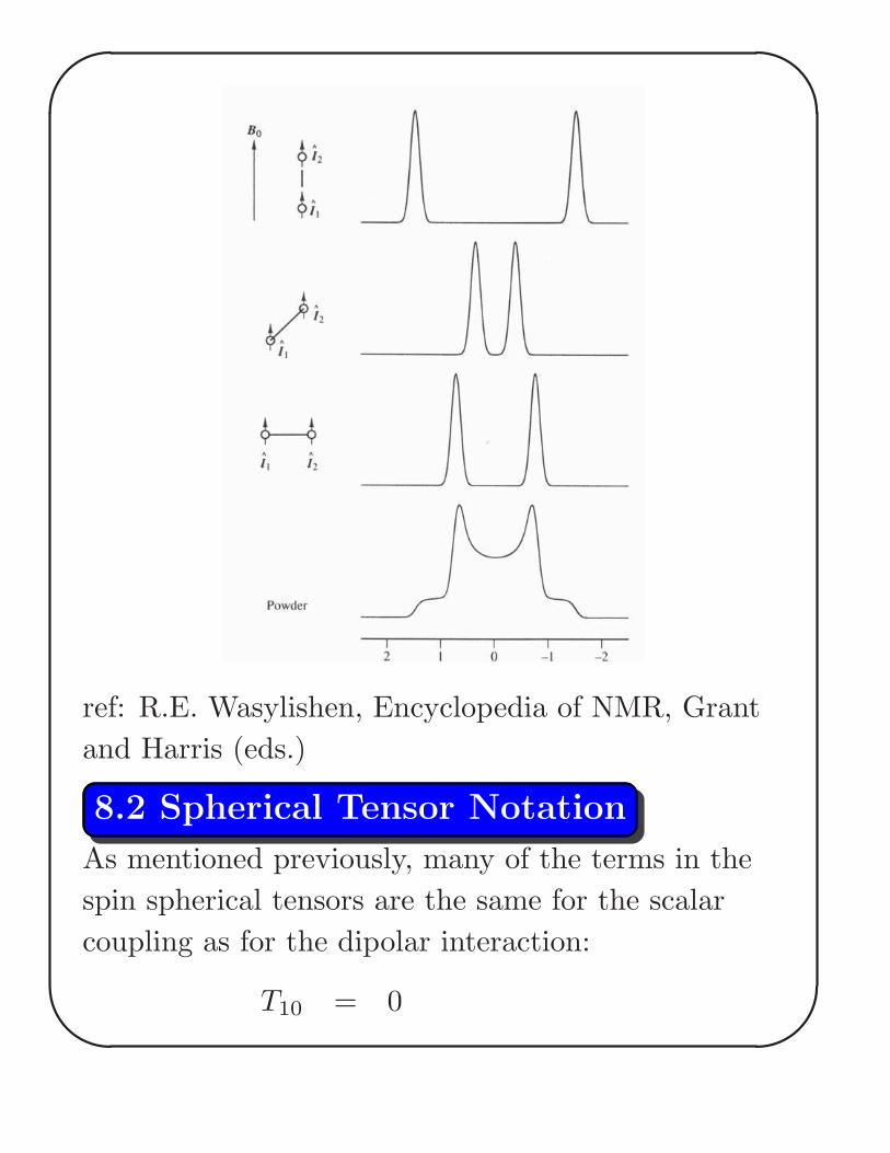
Note that since the static magnetic field lies along
the z-axis in the figure on page 1, the dipolar
'
&
$
%
interaction has an orientational dependence with
respect to ~B0 given by the expression 3cos2θ − 1.
This manifests itself by a dependence of the observed
dipolar splitting on the orientation of the crystallite
in a single crystal in the probe (recall the orientation
dependence of the CSA for single crystals). For a
powder sample, a Pake pattern, which is the sum of
the spectra of individual crystallites which are
randomly distributed in the sample, is observed.
The maximum splitting which can be observed is
3 ∗ dII for the homonuclear case and 2 ∗ dIS for the
heteronuclear case.
'
&
$
%
ref: R.E. Wasylishen, Encyclopedia of NMR, Grant
and Harris (eds.)
8.2 Spherical Tensor Notation
As mentioned previously, many of the terms in the
spin spherical tensors are the same for the scalar
coupling as for the dipolar interaction:
T10 = 0
'
&
$
%
T1±1 = 0
T20 =1√6(3IzSz − I · S)
T2±1 = ∓1
2(IzS± + I±Sz)
T2±2 =1
2I±S±
(8.18)
Note, that here I chose to write the two spins as I
and S instead of I1 and I2, as above. Both notations
are equivalent. The choice depends on you.
The spatial parts are:
APAS20 =
√6dIS
A2±1 = 0
A2±2 = 0
(8.19)
where
dIS = −µ0
4π
γIγS h
r3IS
(8.20)
is the dipolar coupling constant.
As before, we can transform the spatial part into any
'
&
$
%
arbitrary frame:
A20 =
√
3
2dIS(3cos2β − 1)
A2±1 = ±3
2dISsin(2β)e∓iγ
A2±2 =3
2dIS(sin2β)e∓iγ .
(8.21)
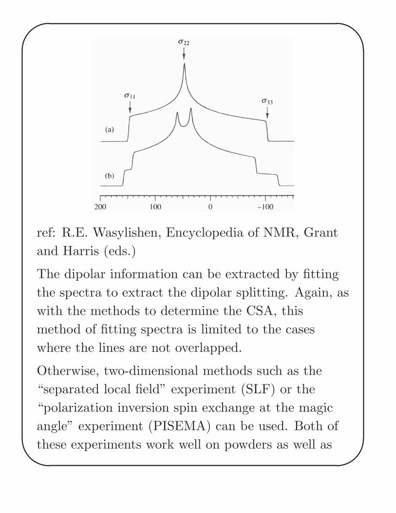
8.3 Measuring the Dipolar Splitting
The dipolar interaction can be measured in a number
of ways. As with the CSA, the methods used depend
on the state of the sample. For a powder, for
instance, one can obtain dipolar information from
the powder pattern directly, as shown in b):
'
&
$
%
ref: R.E. Wasylishen, Encyclopedia of NMR, Grant
and Harris (eds.)
The dipolar information can be extracted by fitting
the spectra to extract the dipolar splitting. Again, as
with the methods to determine the CSA, this
method of fitting spectra is limited to the cases
where the lines are not overlapped.
Otherwise, two-dimensional methods such as the
“separated local field” experiment (SLF) or the
“polarization inversion spin exchange at the magic
angle” experiment (PISEMA) can be used. Both of
these experiments work well on powders as well as
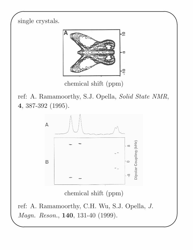
'
&
$
%
single crystals.
chemical shift (ppm)
ref: A. Ramamoorthy, S.J. Opella, Solid State NMR,
4, 387-392 (1995).
chemical shift (ppm)
ref: A. Ramamoorthy, C.H. Wu, S.J. Opella, J.
Magn. Reson., 140, 131-40 (1999).
'
&
$
%
For more details on dipolar spectroscopy see also:
1. M. Engelsberg, Encyclopedia of NMR, Grant
and Harris (eds.).
2. K. Schmidt-Rohr, H.W. Spiess, Mutlidimensional
Solid-State NMR and Polymers, Academic Press,
San Diego, CA, 1994.
8.4 Importance of the Dipolar Interaction
1. In solution, though the dipolar interaction is
averaged (because all θ’s are sampled), it still
plays a role in cross-relaxation and is used in
NOESY spectroscopy - more on this later.
Relaxation.
2. In solids, the dipolar interaction is used to get
distance and orientational information:
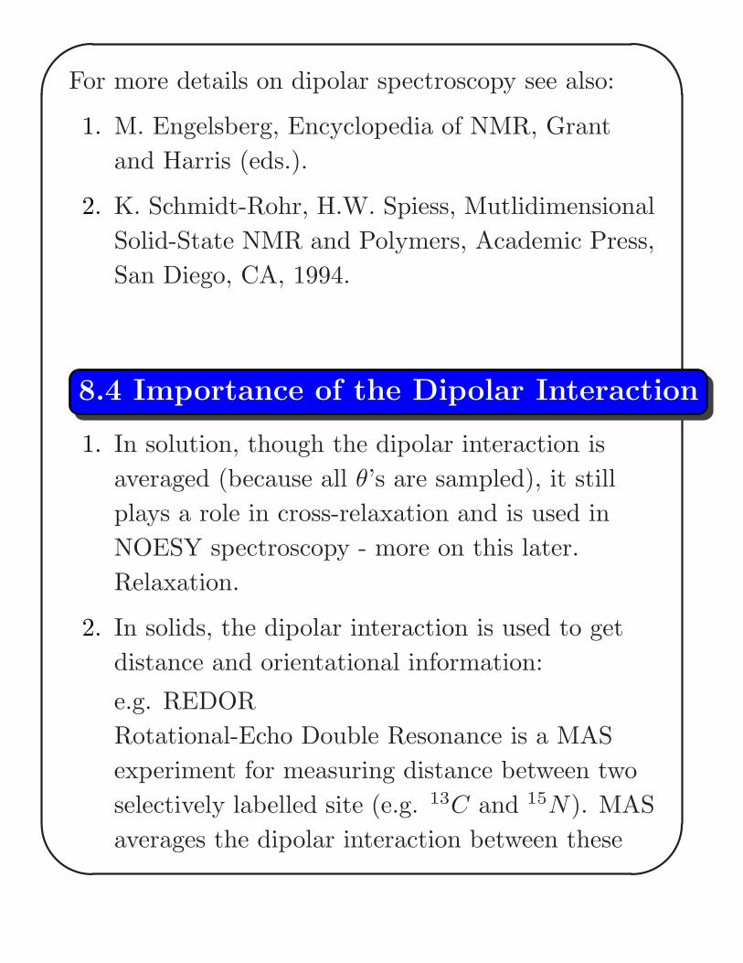
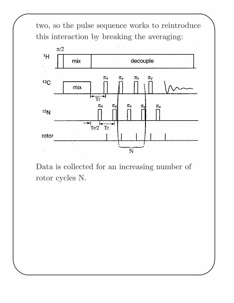
e.g. REDOR
Rotational-Echo Double Resonance is a MAS
experiment for measuring distance between two
selectively labelled site (e.g. 13C and 15N). MAS
averages the dipolar interaction between these
'
&
$
%
two, so the pulse sequence works to reintroduce
this interaction by breaking the averaging:
Data is collected for an increasing number of
rotor cycles N.
'
&
$
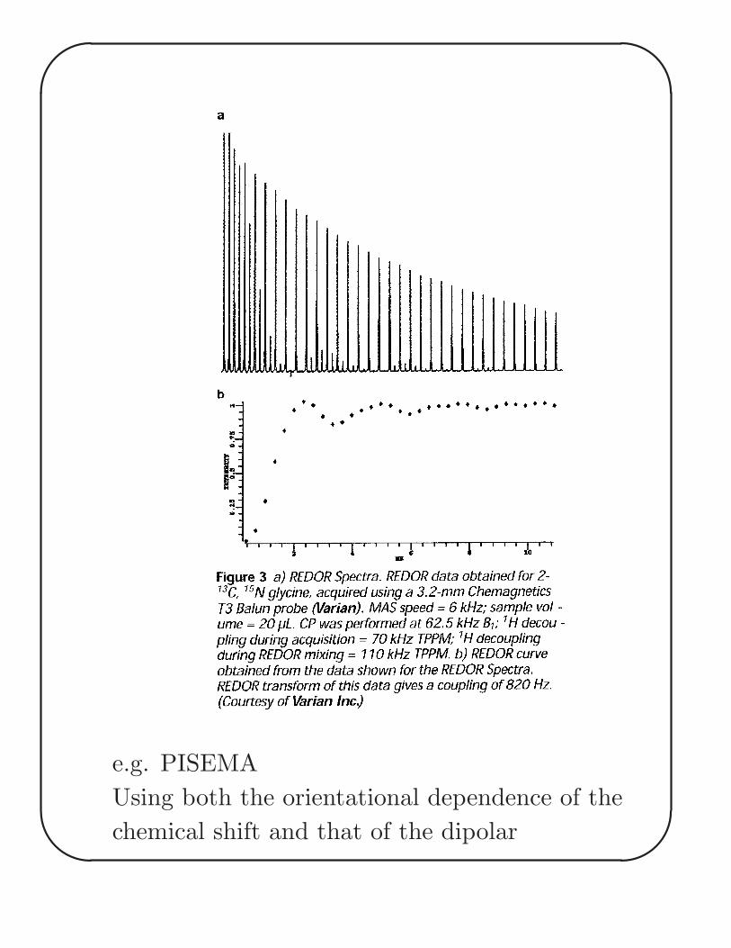
%e.g. PISEMA
Using both the orientational dependence of the
chemical shift and that of the dipolar
'
&
$
%
interaction, it is possible to determine the
three-dimensional structure of an aligned protein
using the PISEMA pulse sequence.


![Kumada Coupling [Mg] - CCC/UPCMLDccc.chem.pitt.edu/wipf/Courses/2320_07_files/Palladium_II.pdf · Kumada Coupling [Mg] ... and reductive-elimination steps and preventing the competing](https://static.fdocument.org/doc/165x107/5aec91a67f8b9a585f8ef7ce/kumada-coupling-mg-ccc-coupling-mg-and-reductive-elimination-steps-and.jpg)