Turbulent, Extreme Multi-Zone Model for Simulating Flux and

Polarization Variability in Blazars

Alan P. Marscher

Institute for Astrophysical Research, Boston University, 725 Commonwealth Avenue,

Boston, MA 02215

marscher@bu.edu

ABSTRACT

The author presents a model for variability of the flux and polarization of

blazars in which turbulent plasma flowing at a relativistic speed down a jet

crosses a standing conical shock. The shock compresses the plasma and accel-

erates electrons to energies up to γmax & 104 times their rest-mass energy, with

the value of γmax determined by the direction of the magnetic field relative to

the shock front. The turbulence is approximated in a computer code as many

cells, each with a uniform magnetic field whose direction is selected randomly.

The density of high-energy electrons in the plasma changes randomly with time

in a manner consistent with the power spectral density of flux variations derived

from observations of blazars. The variations in flux and polarization are therefore

caused by continuous noise processes rather than by singular events such as ex-

plosive injection of energy at the base of the jet. Sample simulations illustrate the

behavior of flux and linear polarization versus time that such a model produces.

The variations in γ-ray flux generated by the code are often, but not always,

correlated with those at lower frequencies, and many of the flares are sharply

peaked. The mean degree of polarization of synchrotron radiation is higher and

its time-scale of variability shorter toward higher frequencies, while the polariza-

tion electric vector sometimes randomly executes apparent rotations. The slope

of the spectral energy distribution exhibits sharper breaks than can arise solely

from energy losses. All of these results correspond to properties observed in

blazars.

Subject headings: galaxies: active — galaxies: jets — polarization — quasars:

general — BL Lacertae objects: general — radiation mechanisms: non-thermal

– 2 –

1. Introduction

The blazar class of active galactic nuclei is characterized by extreme variability of flux

and polarization of nonthermal radiation across the electromagnetic spectrum. Statistical

analyses of the flux variations — in particular, the power-law power spectra (Chatterjee et

al. 2008, 2009, 2012; Abdo et al. 2011) — imply that the variations are governed by noise

processes with higher amplitudes on longer time-scales. Furthermore, the linear polarization

of blazars ranges from a few to tens of percent and tends to be highly variable in both degree

and position angle (e.g., D’Arcangelo et al. 2007; Marscher et al. 2010; Itoh et al. 2013).

Although the range of degree of polarization and the tendency for the position angle to be

similar to or nearly transverse to the jet axis (e.g., Jorstad et al. 2007) can be explained with

a helical magnetic field (Lyutikov et al. 2005; Pushkarev et al. 2005), the rapid variations

in polarization are not naturally reproduced in a model in which the field is either 100%

globally ordered or completely chaotic on small scales. In the former case, the ordered field

provides stability to the polarization, while in the latter case the polarization cancels in the

presence of an essentially infinite number of random field directions.

A natural explanation for the noise-like fluctuations of flux and polarization in blazars

is the presence of turbulence in the relativistic jets that emit the nonthermal radiation. If

one approximates the pattern of the turbulence in terms of N cells, each with a uniform

magnetic field with random orientation, the degree of linear polarization has a mean value

of 〈Π〉 ≈ ΠmaxN−1/2, where Πmax, typically between 0.7 and 0.8, corresponds to the uniform

field case (Burn 1966). If the cells pass into and out of the emission region, the polarization

will vary about the mean with a standard deviation σΠ ≈ 0.5ΠmaxN−1/2 (Jones 1988). The

electric-vector position angle (EVPA) χ of the polarization will also change with time in a

random manner that can often appear as a rotation over hundreds of degrees (Jones 1988;

Marscher et al. 2008; D’Arcangelo 2009).

The superposition of ordered and turbulent magnetic field components can provide the

combination of a preferred orientation of the polarization vector plus fluctuations in Π and

χ. Here the author introduces a numerical model that creates this combination by passing

turbulent cells through a standing shock wave. Daly & Marscher (1987), Cawthorne & Cobb

(1990), Gomez et al. (1995), and D’Arcangelo et al. (2007) have proposed that a stationary

conical shock caused by a pressure mismatch with the external medium corresponds to the

bright compact structure (the “core”) observed at the upstream end of blazar jets imaged

with very long baseline interferometry (VLBI) at millimeter wavelengths. In this spectral

range, relatively low optical depths allow jets of many blazars to be viewed on sub-parsec

scales with minimal obscuration by synchrotron self-absorption.

The following two sections describe the physical model and a numerical code that im-

– 3 –

plements the model. This “Turbulent Extreme Multi-Zone” (TEMZ) code calculates, as a

function of time, the spectral energy distribution (SED) from synchrotron radiation and in-

verse Compton (IC) scattering, as well as the linear polarization of the synchrotron emission

at various frequencies. Seed photons for the scattering include infrared emission by hot dust

in a parsec-scale molecular torus, as well as synchrotron and IC photons from a Mach disk

(MD) on the jet axis. The MD, often called a “working surface” when it occurs near the end

of a jet, is a strong shock oriented transverse to the jet axis that forms near the apex of a

conical shock when the jet maintains azimuthal symmetry (Courant & Friedrich 1976).

After the description of the model in §2, §3 briefly reviews the tests carried out to check

the accuracy of the numerical code. Section 4 presents the results of a small number of

numerical simulations that serve as illustrations of the variability patterns that the model

generates, while §5 presents the conclusions of this work. A future study will include a more

complete exploration of parameter space.

2. Description of the TEMZ Model and Numerical Code

The author has developed a numerical code designed to simulate the time-dependent

SED from a relativistic jet in which turbulent plasma crosses a standing conical shock plus

Mach disk. (The code, originally written in the Fortran-77 computer language, has also

been translated to the C++ language by M. Valdez.) The run time on a common desktop or

laptop computer with a Linux operating system is hours or days, depending on the number

of emission zones (“cells”), values selected for the physical parameters, and the number of

simulated time steps involved (hundreds to thousands). The program calculates the SED

from 1 × 1010 to 5.6 × 1026 Hz, with four frequencies per decade, as well as the degree and

position angle of linear polarization (for synchrotron radiation only) at each time step.

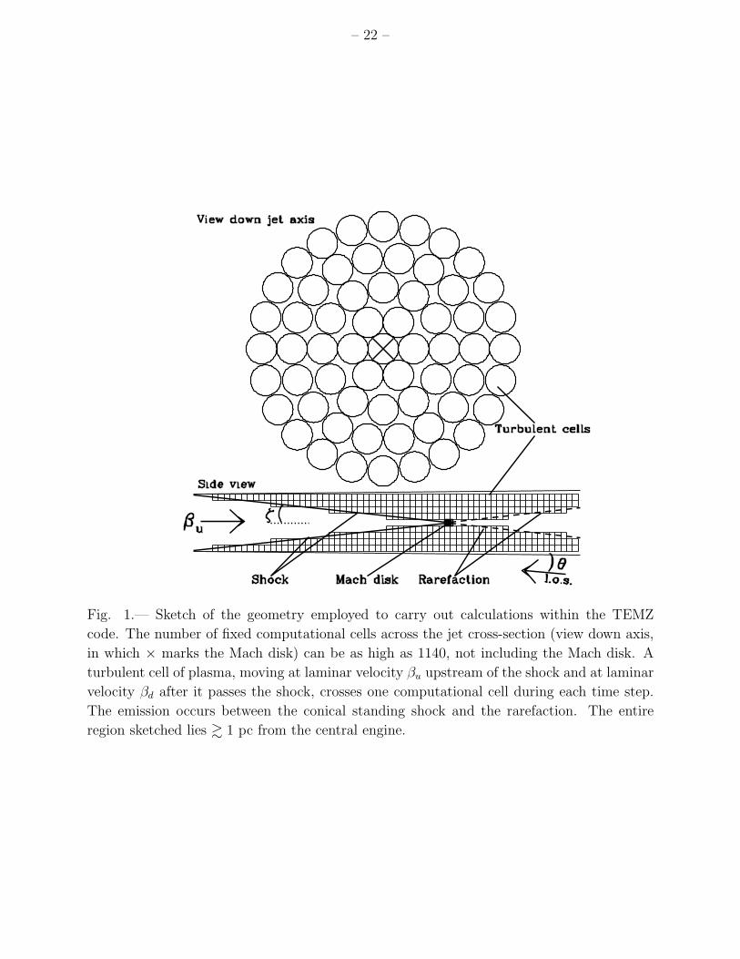
As depicted in Figure 1, the TEMZ geometry consists of many cylindrical computational

cells, fixed in space, through each of which a single turbulent cell of plasma passes during one

time step. The plasma contains magnetic field and relativistic electrons (and positrons, if

any), as well as protons that are presumed not to contribute a significant amount of radiation.

The field is uniform within any given turbulent cell. The plasma flows downstream, i.e., ra-

dially away from the central engine, through the computational cells at a laminar relativistic

velocity βdc, where c is the speed of light and the subscript “d” refers to the region down-

stream of the shock. The corresponding bulk Lorentz factor is defined as Γd ≡ (1− β2d)

−1/2.

The plasma within each turbulent cell has a turbulent component βtc of the bulk velocity,

with a randomly selected direction relative to the systematic flow. For simplicity, and be-

cause of the high Lorentz factor at which the fluid is advected downstream, the turbulent

– 4 –

component of the bulk velocity is subsequently held constant. Also for simplicity, the model

approximates that there is no physical interaction between adjacent cells.

The radiating electrons (as well as any positrons) are accelerated to relativistic energies

as the plasma crosses a conical “recollimation” shock, oriented such that it narrows with

distance from the central engine. A Mach disk can be present at the apex of the conical

shock. Beyond the apex, the flow crosses a conical rarefaction that causes the flow to expand

and accelerate. The current version of the code assumes that the emission turns off after

the plasma crosses the rarefaction. While this may not be the case at lower frequencies

given the long time-scales for energy losses by the radiating electrons, the assumption lowers

the computing time considerably. Hence, the accuracy of the results presented here may

decrease toward centimeter wavelengths, where the flux density is generally higher than that

calculated in the TEMZ code. In many blazars, the flux at such wavelengths is dominated

by features well downstream of the “core” structure treated by the TEMZ model.

Figure 1 sketches the geometry, as viewed both down the axis and from the side, of the

section of the jet over which the calculations are performed. (Note that the geometry of

the computational cell structure is approximated to be cylindrical. This ignores the slight

spreading of the jet expected from the small transverse components of both the laminar and

turbulent velocities. These components are included in the calculation of Doppler factors

described below, however.) The time step, in the observer’s frame, is selected as the time

required for a turbulent cell of plasma to move downstream by one computational cell length

ℓ = 0.2Rcell/ tan ζ, where the cell cross-sectional radius Rcell is selected by the user and

ζ, also a free parameter (although subject to constraints; see below), is the angle between

the conical shock front and the jet axis. The factor of 0.2 corresponds to 2 divided by the

number of cells (10) in an outer column (where the “columns” are parallel to the jet axis)

between the start of that column and the start of the neighboring column (see Fig. 1).

The energy density of relativistic electrons ue in the upstream, unshocked plasma fluc-

tuates about a nominal value u∗e set by the user, modulated randomly with time within a

distribution that reproduces a power spectral density (PSD) of flux variations with a power-

law shape. A subroutine supplied by R. Chatterjee (see Chatterjee et al. 2008), based on the

algorithm of Timmer & Konig (1995), produces 2n random values between −1 and 1 that

correspond to a power-law PSD with a slope provided by the user, where n is an integer.

Following a suggestion by Uttley et al. (2005), the TEMZ code exponentiates each number

produced by the subroutine in order to derive the multiplicative factor that is applied to

the input value of the energy density. (A new, improved prescription by Emmanoulopoulos

et al. 2013, for producing the fluctuations will be incorporated in the future.) This is done

for 217 = 131, 072 times, which is sufficient to allow calculations over the desired number of

– 5 –

time steps included in the light curves while taking into account light-travel delays across

the grid of cells. The code averages the fluctuations that are thereby produced over ten time

steps, an action that is necessary because of the discreteness of the cell arrangement (see

the previous paragraph). [The current version of the code includes gradients in unshocked

energy density only in the longitudinal direction (through the time dependence), not in the

transverse direction.] For the same reason, the orientation of the unshocked magnetic field

vector is selected at random every ten time steps, i.e., for every tenth turbulent cell along

a given column. Within the intermediate cells, the unit vector defining the direction of the

field is rotated smoothly between the previous and next randomly selected directions, along

either the longest or shortest path of rotation (selected randomly with 50% probability for

each). This procedure smooths the discrete changes in field direction and prevents unphysi-

cal discontinuities in the magnetic field vector along any given column. (There is, however,

no relation between the directions of the unshocked magnetic field lines in adjacent cells of

different columns in the current version of the code.) The magnetic field strength B is deter-

mined via an assumption that the upstream magnetic energy density is a constant fraction

fB of the nominal electron energy density u∗e,

uB = B2/(8π) = fBu∗e. (1)

(The code contains an option, not implemented in the calculations presented here, that allows

the magnetic energy density to fluctuate with time such that it is always proportional to ue.)

All energy densities, magnetic fields, electron energies, and electron energy distributions are

evaluated in the plasma rest frame unless otherwise indicated.

At every time step, electrons are injected into the cells immediately beyond the shock.

The injection is in the form of a power-law energy distribution with slope −p and low-energy

cutoff γ0,min, both chosen by the user. The high-energy cutoff γ0,max falls within a range from

γ∗max,low to γ∗max,high also set by the user, but with a value within this range that is either:

(1) equal to γ∗max,high(B‖/B)2 (but not less than γ∗max,low), where the subscript ‖ indicates

the component of the magnetic field that is parallel to the shock normal; or (2) selected

at random within a power-law distribution (with slope as an input parameter). The first

option, selected for the calculations presented below, is meant to represent in a crude manner

the higher efficiency of particle acceleration by shocks when B is nearly parallel to the shock

normal and when plasma turbulence is mild. The latter means that the scattering length of

electron motions is too long for particles to cross the shock front many times when the field

is more inclined to the shock normal. (See, e.g., Summerlin & Baring 2012, for simulations

and a discussion related to this.)

The compression ratio η of the conical standing shock follows the expression given by

– 6 –

Cawthorne & Cobb (1990), which is derived from Lind & Blandford (1985):

η = Γuβu sin ζ(8β2u sin2 ζ − Γ−2

u )1/2(1 − β2u cos2 ζ)−1/2. (2)

Here, βu and Γu are the speed in light units and Lorentz factor, respectively, of the bulk

flow upstream of the shock, and η is defined as the ratio of the density of the shocked to

unshocked plasma. (Note that the latter is the inverse of the definition used by Cawthorne

& Cobb 1990). In order to satisfy the criterion for a shock, the angle ζ that the shock front

subtends to the jet axis must satisfy the criterion sin ζ > (√

2βuΓu)−1 for an ultra-relativistic

equation of state. On the other hand, if the value of ζ is too large, the shock decelerates

the flow so much (the downstream velocity component parallel to the shock normal drops to

βd,‖ = 1/3) that the effects of relativistic beaming become weak, contrary to the inference

that beaming of the emission is particularly strong in blazars.

The shock compresses the component of the magnetic field that is perpendicular to the

shock normal by a factor of η. The magnetic field B is calculated in the plasma rest frame,

which changes after the plasma crosses the shock. In order to calculate the downstream

value of B, the code transforms the upstream field to the standing shock frame (which is the

same as the rest frame of the host galaxy), applies the compression factor to the component

perpendicular to the shock normal, and then transforms the field to the rest frame of the

downstream plasma (see Lyutikov et al. 2003).

2.1. Evolution of the Electron Energy Distribution Downstream of the Shock

After the power-law injection of relativistic electrons as plasma crosses the shock front,

the code follows the evolution of the energy distribution as the electrons lose energy via

radiative losses. The jet opening angle φ is assumed to be so small (see Jorstad et al. 2007;

Pushkarev et al. 2012) that expansion cooling is not important within the section of the jet

under consideration. The code employs the standard formula (e.g., Pacholczyk 1970) for the

decrease of energy (in rest-mass units) γ with time:

γ = −kr(B2 + 8πuph)γ

2, (3)

where kr = 1.3 × 10−9 erg−1 s−1 cm3. Here, uph is the energy density of seed photons

that are subject to inverse Compton scattering off the electrons. The formula assumes that

scattering of the electrons off magnetic irregularities randomizes the pitch angles many times

over the energy-loss time-scale, and that the field of seed photons is isotropic in the rest frame

of the plasma. The code calculates uph for each cell at each time step, but only includes

photon energies that fall below the Klein-Nishina limit, beyond which the scattering efficiency

– 7 –

decreases such that the energy losses are much lower than given by the above equation. Both

this approximation and the isotropy assumption lead to a modest sacrifice in accuracy while

allowing an analytical calculation of the electron energy spectrum as a function of time,

which greatly reduces the time required for computations. The seed photons arriving at a

given cell comprise both the steady source of IR emission from a dust torus and time-variable

emission from the Mach disk. Calculation of the latter is carried out for an earlier time, when

the photons arriving at the cell left the MD.

Since the plasma advects beyond the shock with a velocity βd ≈ 1, the distance zloss(γ)

beyond the shock that contains electrons of energy γ is inversely related to γ:

zloss(γ) = (7.5 erg cm−3)(B2 + 8πuph)−1[γ−1 − γ−1

0,max]Γd pc, (4)

where the last term accounts for length contraction in the plasma frame (Marscher & Gear

1985). This equation can be inverted to find the maximum energy γmax(z) retained by

electrons after they cross a distance (z − zs)pc beyond the shock front, which is located at

longitudinal position zs:

γmax(z) =γ0,max

1 + (0.13 erg−1 cm3)(B2 + 8πuph)(z − zs)pcΓ−1d γ0,max

. (5)

A similar equation for the lowest electron energy replaces γmax(z) by γmin(z) and γ0,max by

γ0,min.

The electron energy distribution within a cell follows the formula for steady injection

of electrons into a volume while radiative losses are operating (Kardashev 1962; Pacholczyk

1970):

N(γ, z) = Q0γ−p

∫ t

0

[1 − kr(B2 + 8πuph)t

′γ]p−2dt′, (6)

where the injected electron energy distribution is a power-law of slope −p, and Q0, which is

related to ue, defines the injection rate. Here, the upper limit t is the lesser of (z−zs)(Γdβdc)−1

and [(γ0,max/γ) − 1][kr(B2 + 8πuph)γ0,max]

−1. For a single cell with injection at one end, the

integral can be evaluated as:

N(γ, z) = Q0[(p− 1)kr(B2 + 8πuph)]

−1γ−(p+1) ×{1 − [1 − kr(B

2 + 8πuph)tγ]p−1}. (7)

This equation is valid for γ0,min ≤ γ ≤ γmax(z) and only for plasma in computational cells

that border the standing shock. For all cells farther downstream than this, the code takes

into account the change in seed photon energy density with time in a given turbulent cell of

plasma as it propagates through the computational cells downstream of the shock. That is,

– 8 –

the value of uph used in equation (7) is the average since the time that the plasma crossed

the shock.

In the MD, where the magnetic field and density of electrons are much higher than in

the plasma that crosses the conical shock, the electrons are in the “fast cooling regime,”

i.e., they radiate most of their energy before crossing one cell length. The ratio of the

photon to magnetic energy density adopted to compute the energy losses of electrons in

the MD plasma follows that calculated by Sari & Esen (2001), uph = εB2/(8π), where

ε = 0.5[√

1 + (4/fB) − 1].

2.2. Calculation of Synchrotron Emission and Absorption

The code computes the synchrotron emission coefficient jν within each cell at every time

step via the standard formula (e.g., Pacholczyk 1970)

jSν (ν ′) =

√3e3

4πmc2B sin ψ

∫ γmax(z)

γmin(z)

N(γ, z)F(ν ′/νc)dγ. (8)

Here, ν ′ is the frequency of the emission in the plasma rest frame, e is the magnitude of the

electron charge, m is the electron rest mass, ψ is the angle between the magnetic field and

the (aberrated) line of sight in the plasma frame, and νc = 2eBγ2/(4πmc) is the synchrotron

critical frequency, averaged over electron pitch angle. The function F(ν ′/νc) is the usual

synchrotron kernel, given in Pacholczyk (1970), for example. The code uses the excellent

approximation for F(ν ′/νc) found by Joshi & Bottcher (2011).

The angle ψ is computed by Lorentz transforming the line-of-sight unit vector s to the

plasma (primed) frame. The coordinates are selected such that s lies in the x-z plane. The

value of B sin ψ is then calculated as |s′×B|.

The TEMZ code calculates the absorption coefficient in each cell in a similar manner,

again using a standard expression (e.g., Pacholczyk 1970):

κSν (ν ′) =

(p+ 2)√

3e3

4πmc2B sin ψ

∫ γmax(z)

γmin(z)

N(γ, z)γ−1F(ν ′/νc)dγ. (9)

The intensity of radiation leaving the cell follows the usual solution to radiation transfer in a

uniform source: Iν(ν′) = [jν(ν

′)/κν(ν′)]{1−exp[−τν(ν ′)]}, where τν equals κν times the path

length through the cell, which is equal to the cell length to a very good approximation for

small angles to the line of sight θlos. If there are next other cells along the line of sight between

the cell of interest and the observer, the intensity is attenuated by a factor of exp[−nextτν(ν′)].

– 9 –

This approximation is employed to conserve computation time. It is roughly valid since the

electrons responsible for absorption have low energies, and thus are not strongly affected by

radiative energy losses. (A more accurate calculation of absorption is under development.)

The flux density from a cell equals the intensity of radiation received from the cell times the

essentially circular area of its face. The total flux density Fν from the source is a simple sum

over that from all cells.

2.3. Calculation of Inverse Compton Emission

For a given spectral intensity Iν′ of seed photons arriving at a cell, the emission coefficient

of IC scattering requires a double integration over electron energy and seed photon frequency.

While it also properly involves a double integral over photon angles, this requires excessive

computing time when many emission zones are involved. The code therefore utilizes the

Klein-Nishina cross-section derived by Dermer & Menon (2009) (eq. 6.31) under the “head-

on” approximation that the photon is scattered in the initial direction of the electron’s

motion:

σKN =3

8σT (y′ + y′ −1 − 2q′ + q′ 2)/(γǫ′i), (10)

where y′ ≡ 1 − (ǫ′/γ), q′ ≡ ǫ′/(γy′ǫ′i), and ǫ′ ≡ hν ′/(mc2), ν ′i is the frequency of the seed

photon, ν ′ is the frequency of the scattered photon, σT = 6.653× 10−25 cm2 is the Thomson

cross-section, and h is Planck’s constant. The cross-section is valid for (1+4γǫ′i)−1 < y′ < 1.

The inverse Compton emission coefficient is then

jICν (ν ′) =

∫ γmax

γ1

∫ ∞

ν′

i,1

I ′seed(ν′i)N(γ, z)σKN(ν ′, ν ′i, γ)dν

′idγ, (11)

where γ1 is the greater of γmin and ǫ′[1 +√

1 + (ǫ′iǫ′)−1]/2, ν ′i,1 = ν ′[4γ2(1 − ǫ′γ−1)]−1, and

I ′seed(ν′i) is the spectral intensity of seed photon emission as measured in the plasma rest

frame.

Equation (10) contains an implicit dependence on the angle between the bulk velocity

vector of the plasma and the direction of the source of seed photons. This results from the

Doppler formula for the transformation of frequency from the rest frame of the seed photon

source (SP) to the plasma frame: ν ′i = νiδSP, where

δSP = [Γrel(1 − βrel cos ϑ′rel]

−1. (12)

Here, βrel is the magnitude of the relative velocity in light units between the plasma and

seed photon source, Γrel is the corresponding Lorentz factor, and ϑ′rel is the aberrated angle

– 10 –

between the velocity vector of the plasma and the aberrated direction of the seed photon

source in the plasma frame.

2.4. Sources of Seed Photons for Inverse Compton Scattering

The current version of the TEMZ code includes two sources of seed photons available

for IC scattering by electrons in the cells: infrared (IR) blackbody emission from hot dust

contained in a patchy molecular torus (external Compton, hereafter “EC-Dust”) and syn-

chrotron plus first-order synchrotron self-Compton emission from a Mach disk (“SSC-MD”)

centered on the jet axis at the narrow end of the conical shock (see Fig. 1). Because of the

relativistic motion of the plasma in the cells, the radiation from both of these sources is

blueshifted and beamed in the plasma rest frame. The code does not currently include the

seed photons from synchrotron emission within the cell under consideration (“SSC”) plus all

of the other cells (“SSC-C”), owing to the excessive computational time required given the

large number of cells. Future parallelization of the C++ version of the code is planned in

an effort to make such calculations possible.

The central circle of the dusty torus lies a distance rt from the center of the system,

assumed to be a black hole (BH), and the torus has a cross-sectional radius Rt. As viewed

from a cell at a polar distance z from the BH, the dusty torus subtends a ring in the sky. In

the rest frame of the system, the direction of the outer/inner boundary of the ring subtends

an angle

ξoutin ≈ tan−1 (rt/z)± sin−1[Rt(z

2 + r2t )

−1/2] (13)

to the direction toward the BH. In the rest frame (primed) of the plasma in the cell, which

moves at velocity βd (Lorentz factor Γd) approximately in the z direction (the slight deviation

from this direction is unimportant for this calculation), each of these angles is transformed

as

tan (ξ′/2) = tan (ξ/2)[Γd(1 + βd)]−1. (14)

The blackbody emission from the torus in the plasma frame corresponds to a temperature

T ′ = δSPT = [Γd(1 − βd cos ξ′)]−1T, (15)

where ξ′ ranges from ξ′in to ξ′out. The code integrates the resultant blackbody spectrum over

the surface area from angle ξin to ξout. The area filling factor of the blackbody emission is set

by the size, temperature, and luminosity of the torus, with the latter derived from the IR flux

observed at the Earth. Direct observations of the dust emission from the quasar 4C 21.35

(Malmrose et al. 2011) guide the choice of these physical parameters. In this γ-ray bright

object, the flux of the dust emission is almost entirely from a single-temperature blackbody

– 11 –

(T ≈ 1200 K) and has a value of 0.22 times the flux of the accretion disk that provides most

of the optical-ultraviolet luminosity. In the case of 4C 21.35, the area filling factor of the

dust emission is ∼ 0.6 pc2/(rtRt) and Rt ≈ 0.22rt.

The code calculates the synchrotron and first-order SSC emission generated by the

plasma in the MD at each time step (see above). Since the cross-sectional size of the MD

is not well specified by gas dynamical theory, it is left as a free parameter (see Table 1).

The plasma decelerates from a high Lorentz factor to Γd ≈ 1.2 as it crosses the MD shock

front, hence the shock greatly magnifies the magnetic field and electron density relative to

the values in other cells. The seed photons from the MD arrive at each cell with a time delay

that depends on the distance of the cell from the MD. The blueshift δMD of the MD photons

in the frame of the plasma in the cell depends on the angle between the cell’s line of sight

to the MD and the velocity vector of the plasma relative to that of the Mach disk plasma,

with the latter assumed to be βMD = 1/3 in the z direction. The flux then depends on

both the inverse square of the distance of the cell from the MD and the relativistic beaming

factor δ2+αMD , where the dependence of the flux density Fν on frequency ν is Fν ∝ ν−α.

(Since α can change with frequency, its value is determined by the code from the emission

calculation.) The synchrotron flux received from the MD also depends on the angle ψMD

that the MD magnetic field subtends to the aberrated line of sight between the cell and the

MD, Fν ∝ (sin ψMD)1+α. The synchrotron self-absorption optical depth within the MD for

radiation that will intersect the cell is proportional to (sin ψMD)1.5+α. The current version of

the code approximates the optical depth of synchrotron self-absorption in intervening cells

by multiplying the absorption coefficient of the cell by the distance between the MD and the

cell.

2.5. Linear Polarization

The current version of the TEMZ code calculates the linear polarization for each cell

in a simple manner. For an optically thin cell, the degree of polarization depends on the

(frequency-dependent) spectral index, Πcell = (α + 1.0)/[α + (5.0/3.0)], with electric-vector

position angle (EVPA) perpendicular to the direction of the magnetic field as projected on the

sky. In the optically thick case Πcell = 3/(12α + 19), and the EVPA is along the projected

direction of the magnetic field (Pacholczyk 1970). These relations are valid because the

magnetic field is treated as uniform within each cell. The code calculates the value of χcell,

aberrated by relativistic motion, following the formulation of Lyutikov et al. (2005). From

the flux density of the cell Fν,cell determined as in §2.2, the Stokes parameters are then set as

Qs,cell = Fν,cell cos 2χcell and Us,cell = Fν,cell sin 2χcell. The code sums Qs,cell and Us,cell over

– 12 –

all of the cells to determine the integrated degree of polarization Π = (Q2s + U2

s )1/2/Fν and

position angle χ = 0.5 tan−1(Us/Qs).

3. Testing of the Numerical Code

Because of the complexity of the algorithms needed to carry out the calculations, the

author has tested the output of the code in a variety of ways. The first set of tests involved

comparison of the synchrotron and IC spectrum computed for single cells, with standard

analytical expressions for a cylindrical source with uniform properties (see, e.g., Pacholczyk

1970). The position angle of linear polarization of the synchrotron emission was tested for

different directions of uniform magnetic fields relative to the shock front and to the line of

sight. The difference in degree and position angle of polarization with shock compression

was compared with the case of no compression. A print-out of the evolution of the electron

energy distribution of a given parcel of plasma provided a check on the numerical handling of

how radiative energy losses affect the distribution. The code passed all of these basic tests.

Testing of the full multi-zone code involved checks on the various time delays for prop-

agation of electromagnetic waves and advection of plasma downstream of the shock. The

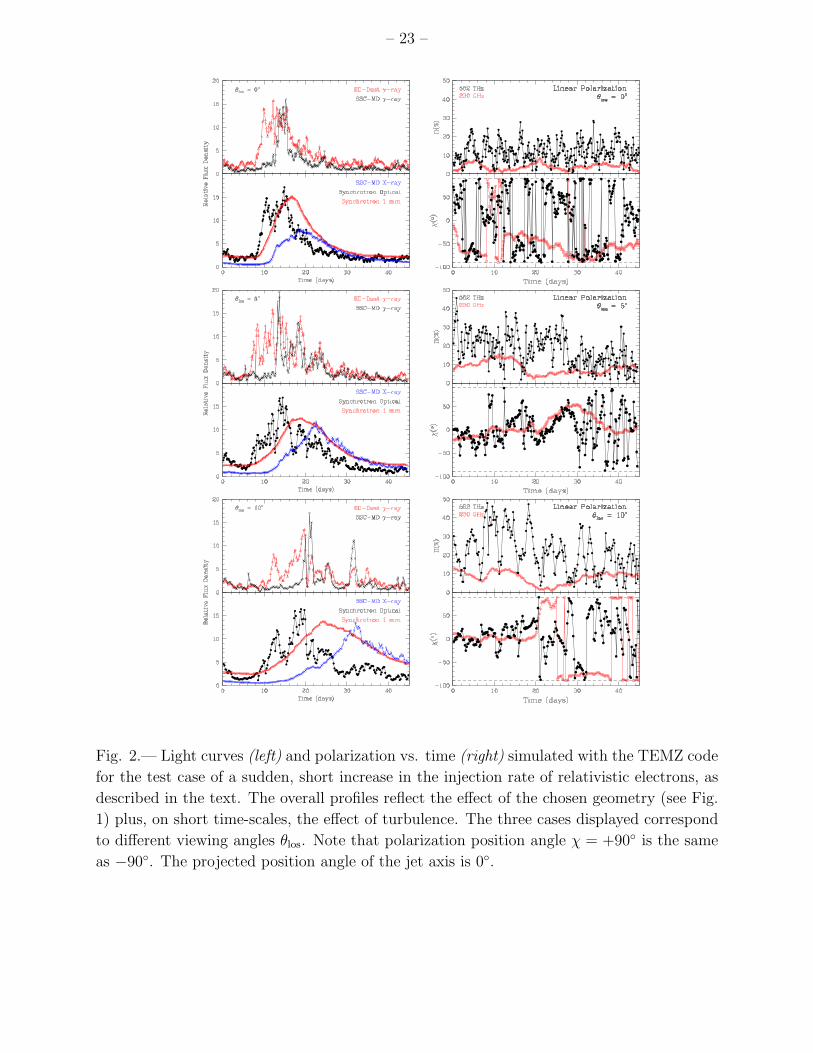
introduction of a very high-amplitude pulse of relativistic electron injection (i.e., a sudden

increase in Q0) over a few time steps facilitated comparison of the time-dependent output

of the code with the expected behavior. Sample results are displayed in Figure 2. Here we

see that, for θlos ≈ 0, the induced optical synchrotron and EC-Dust flux rises steeply as the

pulse crosses the ring of computational cells at the upstream end of the shock, then declines

more gradually as the pulse crosses smaller rings of cells. (The electrons that produce γ-ray

and optical photons lose energy rapidly, hence radiation at these frequencies is confined to

a thin layer close to the shock.) The SSC-MD flux increases modestly at first before a rapid

flare occurs as the pulse crosses the MD, creating a sudden increase in seed photon flux.

4. Results of Sample Numerical Simulations

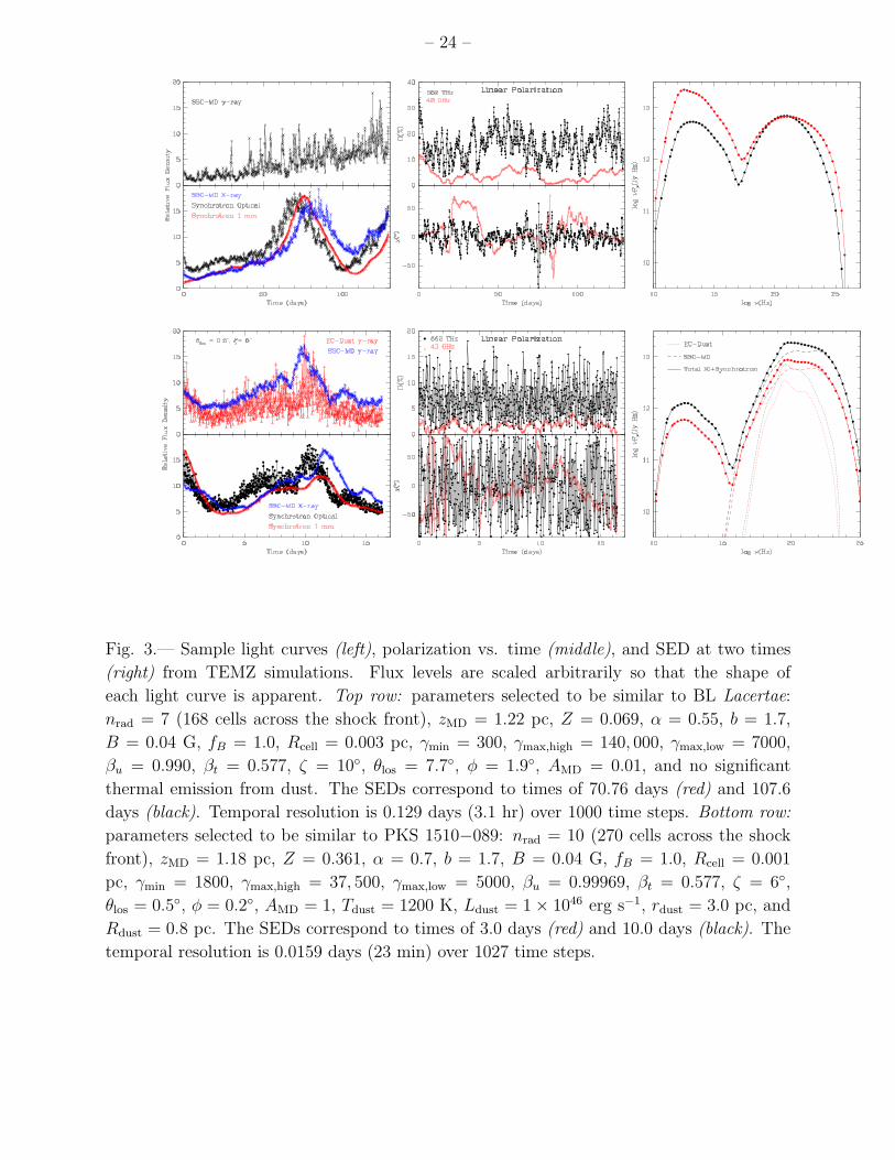
Figure 3 presents samples of light curves, polarization vs. time, and SEDs for two of

the TEMZ simulations. The parameters were selected to be similar to those of two blazars,

BL Lacertae and PKS 1510−089, as derived from observations (e.g., Jorstad et al. 2005;

Marscher et al. 2008, 2010). They are not intended, however, as actual fits to any data.

In fact, because of the randomness inherent in the model, close fits to observational data

cannot be attained. Rather, future success of the model will depend on comparison of the

– 13 –

statistical characteristics of the simulated results with those of the data.

The BL Lac-like simulation bears a resemblance to the observed flux and polarization

versus time curves of this blazar presented in Marscher (2013). The running mean of the

γ-ray flux level increases with time, while on short time-scales the flux varies erratically. The

fluxes at lower frequencies rise and fall roughly together, although with some cross-frequency

delays in maxima and minima. The fluctuations about the running mean at optical and X-ray

frequencies occur on similar time-scales as at γ-ray energies, but with lower amplitudes, while

the variations at λ1 mm (230 GHz) are quite smooth owing to the larger volume occupied by

electrons that emit at this wavelength relative to those responsible for the optical emission.

There are “orphan” (i.e., with no counterpart at the other wavebands) γ-ray flares (e.g., at

t ∼ 30 days) and optical flares without γ-ray counterparts (e.g., at t ∼ 46 days). The higher

amplitude of the γ-ray variations relative to those at optical frequencies results both from

the somewhat higher (factor of ∼ 2-3) energies — and therefore shorter radiative lifetimes

— of electrons that produce γ-rays than those that produce optical synchrotron radiation,

as well as variations in seed photon energy density throughout the emission region owing to

changing conditions in the MD. Since IR emission by hot dust has yet to be confirmed in

a BL Lac object, the simulation includes no contribution to the seed photon field from this

component.

The simulation of a blazar similar to the quasar PKS 1510−089 (bottom row of Fig.

3) produces SSC-MD γ-ray and synchrotron optical light curves that are quite similar, al-

though not identical, in profile. The EC-Dust γ-ray flux varies more erratically because

the electrons that scatter the dust-emitted photons to γ-ray energies are near the highest

energies generated by the shock, and therefore occupy a small fraction of the total volume.

Such high energies result from the lower mean frequency of the seed photons from the dusty

torus relative to the synchrotron and SSC emission from the MD. [Note that the calculation

of the seed photon field includes integration over the torus (see §2.4), rather than the crude

(unless the opening angle of the torus is very large) approximation that the dust-emitted

photons are isotropic in the quasar rest frame at the position of the jet plasma, as approxi-

mated, for example, by Ghisellini & Tavecchio (2009).] The X-ray and λ1 mm light curves

are well-correlated, as observed (e.g., Marscher et al. 2010), although they do not follow each

other completely.

Many of the flares have quite sharp peaks, with rises and decays that are approximately

linear or exponential. This is a common characteristic of blazar light curves (e.g., Chatterjee

et al. 2012) that is difficult for many models to reproduce. The time-scales of the varia-

tions, especially at optical and γ-ray frequencies, can be extremely short, as anticipated by

Marscher & Jorstad (2010) and Narayan & Piran (2012). This is a result of the combination

– 14 –

of (1) the small volume filling factor of production of the highest energy electrons, (2) the

short radiative lifetimes of these electrons, (3) the high Lorentz factor of the laminar flow,

and (4) the turbulent peculiar velocities βt, which can increase the Doppler factor by as

much as a factor of (1 − β2t )

−1/2.

The dependence of the volume filling factor on frequency leads to two additional features

of the model that compare well with observations (see Jorstad et al. 2007; Marscher &

Jorstad 2010; Wehrle et al. 2012; Jorstad et al. 2013). The time-averaged degree of linear

polarization increases, and the time-scale of variability of both the degree and position

angle of polarization decreases while the amplitude of variability increases, with frequency.

Furthermore, breaks in the spectrum by more than by 0.5 (expected from radiative losses in

a single emission zone; e.g., Marscher & Gear 1985) appear at IR and γ-ray frequencies.

As with the light curves, the polarization versus time curves in Figure 3 (middle panels)

also exhibit a combination of systematic and erratic behavior. As expected, the optical

polarization (represented in the figure by 562 THz, or 534 nm, which is within the V band)

ranges from close to zero up to tens of percent for the BL Lac-like simulation and up to nearly

20% for the quasar-like simulation, similar to the observed range (see Marscher et al. 2010;

Marscher 2013, to compare with data). The mean EVPA fluctuates about the jet direction (0◦

in the simulations), as is generally observed in BL Lac. Apparent rotations of the polarization

vector occur, although a larger number of simulations is needed to determine whether they

resemble the variety of such rotations that are observed in blazars (e.g., Marscher et al. 2008;

Larionov et al. 2008; Abdo et al. 2010; Larionov et al. 2013). Such rotations are common

when the degree of polarization is low (see also Jones 1988; Marscher, Gear, & Travis 1992).

If the randomness in the magnetic field directions causes the polarization integrated over

N −M of the cells to cancel, with N ≫ M, the net polarization is low and determined by

the other M cells. Since a small number of cells is involved, time variations can occur that

resemble rotations of the polarization vector. However, such apparent rotations are unlikely

to explain the systematic optical EVPA rotations reported in BL Lac (Marscher et al. 2008)

and PKS 1510-089 (Marscher et al. 2010). Both of these observed events occurred prior to

the time when the emitting plasma crossed the core, and hence took place upstream of the

location where the TEMZ calculations apply. Despite the slower variations of polarization at

longer wavelengths, rotations of the polarization vector still occur at millimeter wavelengths

both in the simulations and in observations (e.g., Larionov et al. 2008).

Both the degree and position angle of the quasar-like simulation vary more erratically

than is typically observed in PKS 1510−089 (e.g., Marscher et al. 2010). This discrepancy

is likely the result of the lack of continuity in the magnetic field vector across cells in the

direction transverse to the jet axis in the current version of the TEMZ code (see §2). Actual

– 15 –

jets may also contain an ordered component of the magnetic field in addition to the turbu-

lent component. If so, the very short time-scale variations in polarization will have lower

amplitudes.

Figure 4 presents sample total (I) and polarized (P ) intensity images at 43 GHz gener-

ated at a particular time of the quasar-like simulation. These images serve as representations

of the brightness and polarization distribution across the source, as well as an indication of

the ability of VLBI observations to test the TEMZ model. In order to generate the images,

a rectangular grid of pixels is set up, with the intensity from all of the cells that lie along

the line of sight represented by each pixel summed (vectorially for a P image) to obtain

the intensity of the pixel. The pixelated image is then convolved with a circular Gaussian

restoring beam (i.e., a point-spread function). The image at the top of the figure is con-

volved with a small beam to reveal the underlying intensity pattern, while the image at the

bottom has a FWHM resolution equal to the diameter of the jet cross-section. The latter is

typical of the angular resolution of the longest baselines of a millimeter-wave VLBI observa-

tion with nearly Earth-diameter maximum separations of antennas. The addition of one or

more space-based antennas is therefore needed in order to determine whether a given blazar

possesses the brightness and polarization structure predicted by the model.

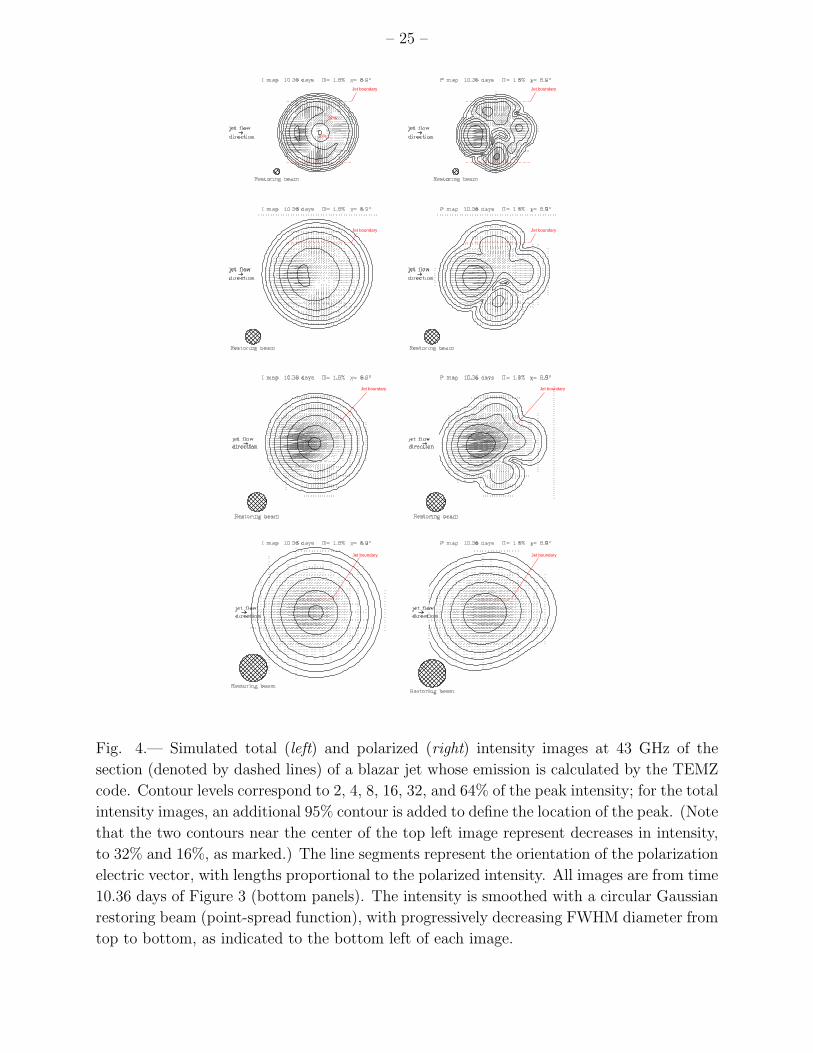
Comparison of the top right and bottom right images in Figure 4 demonstrates that the

low net polarization at 43 GHz is caused by cancellation of cross-polarized sections, which

is nearly complete for very small viewing angles because of the underlying symmetry of the

conical shock structure. The deviation from perfect symmetry between the top and bottom

halves of the images is caused by the random elements in the TEMZ model. Except for this

effect, which is small at 43 GHz owing to the large number of cells that emit at this frequency,

the polarized intensity structure is similar to that calculated and displayed by Cawthorne

(2006), Nalewajko (2009), and Cawthorne et al. (2013). These authors consider the somewhat

different case of a standing shock compressing a magnetic field that is completely chaotic

upstream of the shock.

5. Conclusions

The many-zone emission model provides much more realistic emission calculations than

do schemes involving a very small number of zones. The TEMZ model, improved in ways

discussed below, therefore holds some promise in explaining the diversity of blazar variability

in multi-waveband flux, polarization, and structure. While this may seem to be at the

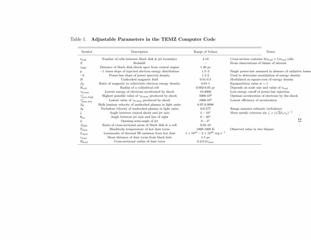
expense of complexity, the number of free parameters, which are listed in Table 1, is similar

to that of single-zone models, with many of the parameters (Z, α, b, βu, θlos, φ, Tdust, and

– 16 –

Ldust) specified by observations. Furthermore, instead of fitting the data to SEDs measured

at a small number of times, the results produced by the TEMZ code can be compared with

the time evolution of the SED as well as the characteristics of the light curves, degree and

position angle of polarization versus time, and total as well as polarized intensity images of

blazars. The author plans to explore how these characteristics as produced by the simulations

depend on the adjustable parameters. This will include timing analyses of the simulated flux

and polarization curves so that the cross-frequency correlations and PSDs can be compared

with those observed in blazars. The results displayed in Figure 3 and discussed in §4 resemble

observations of blazars well enough to warrant such a study.

There is, on the other hand, one aspect of the simulations that conflicts with the data:

the ratio of γ-ray to X-ray luminosity (right-most panels of Fig. 3) is not as high as observed

during major outbursts of some of the most prominent γ-ray bright quasars. This problem

with the simulations was pointed out by Wehrle et al. (2012), who used the TEMZ code to fit

the SEDs of the quasar 3C 454.3 during a major outburst. The over-production of X-rays in

the model is caused by the strong synchrotron emission from the MD at far-IR wavelengths,

as viewed in the rest frame of the plasma in the other cells. Perhaps a more refined treatment

of the MD, based on magneto-hydrodynamic (MHD) simulations (see below), will solve this

problem. On the other hand, a thermal spectrum of seed photons, which declines sharply (as

ν2) toward low frequencies, does not produce an X-ray excess as long as γ0,min & 100. The

high γ-ray to X-ray flux ratio is one reason why seed photons from thermal emission from

broad emission-line clouds and a dusty torus is favored by many authors (e.g., Ghisellini &

Tavecchio 2009). However, at distances & 3 pc from the central engine, the seed photon

field from these regions is too weak to explain the high γ-ray luminosity. If, instead, some

stray molecular clouds or dense, ionized clouds are located along the periphery of the jet, it

is possible that they could produce a sufficient density of seed photons to explain the γ-ray

emission from IC scattering (Leon-Tavares et al. 2013; Isler et al. 2013). The author plans

to add such a source of seed photons to the code. Also, in order to simulate blazars with

ratios of γ-ray to infrared luminosities closer to unity, development of a full SSC and SSC-C

calculation, with seed photons from all of the cells (calculated in retarded time), is underway.

It is likely that, in many blazars, other physical processes besides a single standing

shock are responsible for energizing electrons to induce flares as well as more quiescent

emission. In fact, there is evidence in a number of blazars for multiple standing features

that could correspond to oblique or conical shocks (e.g., Jorstad et al. 2005). The TEMZ

model could be applied separately to emission from any such stationary structures, although

if there is a non-conical shock, the code would need to be altered accordingly. Moving

shocks in a jet filled with turbulent plasma (Marscher, Gear, & Travis 1992) are possible

as well, especially when a very bright superluminal knot is observed to propagate down the

– 17 –

jet. Magnetic reconnections have been proposed as an alternative to shocks as a primary

process for accelerating electrons, causing relativistic bulk motions of plasma, and therefore

generating flares (e.g., Giannios et al. 2009). The TEMZ code can potentially be modified to

incorporate this scenario after studies of relativistic reconnection elucidate how the magnetic

field topography and electron energy distribution vary with time and position.

While randomness in the magnetic field direction in different turbulent cells can cause

observed rotations in the linear polarization vector, it probably does not explain the sys-

tematic rotations observed in some blazars. The conclusion that such events occur before a

disturbance in the jet reaches the standing shock implies that the variable emission described

in the TEMZ code does not cover all of the events in the light curves of blazars. This is also

true at lower frequencies where much of the emission comes from regions farther downstream

in the jet, and even in some cases at γ-ray energies where observations indicate that flares

can take place many parsecs from the core (Agudo et al. 2011a,b). Nevertheless, there is

strong evidence that most of the multi-waveband outbursts in blazars are associated with

emission in the core region treated in the TEMZ model (Marscher et al. 2012).

Despite the promising results presented here, more realistic simulations are needed to

confront the model with data in a serious way. The geometry and physical properties of the

standing shock and Mach disk system are simplified in the current version of the TEMZ code.

Ideally, they should be determined instead by relativistic MHD simulations. The energization

of relativistic electrons is also treated in an ad hoc manner, as is the approximation to

turbulence. Furthermore, the fluctuations in electron energy density are forced to agree with

the observed PSD of blazar flux variations, while they ideally should be dictated by successful

simulations of flow from the accreting black hole system into the jet. The author plans to

collaborate with other groups working in these areas to combine the TEMZ emission code

with detailed calculations of the dynamics and plasma physics of relativistic jets in order to

produce more realistic simulations of emission from blazar jets.

The author thanks R. Chatterjee for providing his code for producing random fluctu-

ations that obey the statistics of a power-law PSD, S. Jorstad, M. Joshi, J. L. Gomez, N.

MacDonald, M. Baring, and M. Bottcher for discussions that were useful in the development

of the model (and the first four plus M. Malmrose for critical readings of a draft version

of the manuscript), M. Valdez for scrutinizing, and identifying some flaws in, the numerical

code and for translating it to C++, and J. L. Gomez for providing visualization software that

aided in testing of the results. He also thanks Prof. Stefan Wagner for his hospitality during

a visit to the University of Heidelberg in 1998 when this study was first conceived. Funding

of this research included NASA grants NNX10AO59G, NNX11AQ03G, and NNX12AO79G,

and NSF grant AST-0907893. This work benefited from discussion within International

– 18 –

Team Collaboration 160 sponsored by the International Space Science Institute (ISSI) in

Switzerland.

REFERENCES

Abdo, A., et al. 2010, Nature, 463, 919

Abdo, A. A., et al. 2011, ApJ, 733, L26

Agudo, I., et al. 2011a, ApJ, 726, L13

Agudo, I., et al. 2011b, ApJ, 735, L10

Burn, B. J. 1966, MNRAS, 133, 67

Cawthorne, T. V. 2006, MNRAS, 367, 851

Cawthorne, T. V., & Cobb, W. K. 1990, ApJ, 350, 536

Cawthorne, T. V., Jorstad, S. G., & Marscher, A. P. 2013, ApJ, 772, 14

Chatterjee, R., et al. 2008, ApJ, 689, 79

Chatterjee, R., et al. 2009, ApJ, 704, 1689

Chatterjee, R., et al. 2012, ApJ, 749, 191

Courant, R., & Friedrich, D. B. 1976, Supersonic Flow and Shock Waves (New York:

Springer-Verlag).

D’Arcangelo, F. D., et al. 2007, ApJ, 659, L107

D’Arcangelo, F. D. 2009, Ph.D. Thesis, Boston University

Daly, R. A., & Marscher, A. P. 1987, ApJ, 334, 539

Dermer, C. D., & Menon, G. 2009, High Energy Radiation from Black Holes: Gamma Rays,

Cosmic Rays, and Neutrinos, Princeton University Press

Emmanoulopoulos, D., McHardy, I. M., & Papadakis, I. E. 2013, MNRAS, 433, 907

Ghisellini, G., & Tavecchio, F. 2009, MNRAS, 397, 985

Giannios, D., Uzdensky, D. A., & Begelman, M. C. 2009, MNRAS, 395, L29

– 19 –

Gomez, J. L., Martı, J. M., Marscher, A. P., Ibanez, J. M., & Marcaide, J. M. 1995, ApJ,

449, L19

Isler, J. C., et al. 2013, ApJ, in press (arXiv:1310.0817)

Itoh, R., et al. 2013, ApJ, 768, L24

Jones, T. W. 1988, ApJ, 332, 678

Jorstad, S. G., et al. 2005, AJ, 130, 1418

Jorstad, S. G., et al. 2007, AJ, 134, 799

Jorstad, S. G., et al. 2013, ApJ, 773, 147

Joshi, M., & Bottcher, M. 2011, ApJ, 727, 21

Kardashev, N. S. 1962, Astron. Zh., 39, 393

Larionov, V. M., et al. 2008, A&A, 492, 389

Larionov, V. M., et al. 2013, ApJ, 768, 40

Leon-Tavares, J., et al. 2013, ApJ, 763,36

Lind, K. R., & Blandford, R. D. 1985, ApJ, 295, 358

Lyutikov, M., Pariev, V. I., & Blandford, R. D. 2003, ApJ, 597, 998

Lyutikov, M., Pariev, V. I., & Gabuzda, D. C. 2005, MNRAS, 360, 869

Malmrose, M., Marscher, A. P., Jorstad, S. G., Nikutta, R., & Elitzur, M. 2011, ApJ, 732,

116

Marscher, A. P. 2013, in 2012 Fermi Symposium, ed. N. Omodel, T. Brandt, & C. Wilson-

Hodge, eConf C121028, arXiv:1304.2064

Marscher, A. P., et al. 2008, Nature, 452, 966

Marscher, A. P., et al. 2010, ApJ, 710, L126

Marscher, A. P., & Gear, W. K. 1985, ApJ, 298, 114

Marscher, A. P., Gear, W. K., & Travis, J. P. 1992, in Variability of Blazars, ed. E. Valtaoja

& M. Valtonen (Cambridge U. Press), 85

– 20 –

Marscher, A. P., & Jorstad, S. G. 2010, in Fermi Meets Jansky — AGN at Radio and

Gamma-Rays, ed. Savolainen, T., Ros, E., Porcas, R.W., & Zensus, J.A. (Bonn:

Max-Planck-Institut fur Radioastronomie), 171

Marscher, A. P., Jorstad, S. G., Agudo, I., MacDonald, N. R., & Scott, T. L. 2012, in Fermi

& Jansky: Our Evolving Understanding of AGN, ed. R. Ojha, D. Thompson, & C.

D. Dermer, eConf C1111101, arXiv:1204.6707

Nalewajko, K. 2009, MNRAS, 395, 524

Narayan, R., & Piran, T. 2012, MNRAS, 420, 604

Pacholczyk, A. G. 1970, Radio Astrophysics (San Francisco: Freeman)

Pushkarev, A. B., Gabuzda, D. C., Vetukhnovskaya, Yu. N., & Yakimov, V. E. 2005, MN-

RAS, 356, 859

Pushkarev, A. B., Lister, M. L., Kovalev, Y. Y., & Savolainen, T. 2012, in Fermi & Jansky:

Our Evolving Understanding of AGN, ed. R. Ojha, D. Thompson, & C. D. Dermer,

eConf C1111101, arXiv:1205.0659

Sari, R., & Esin, A. A. 2001, ApJ, 548, 787

Summerlin, E. J., & Baring, M. G. 2012, ApJ, 745, 63

Timmer, J., & Konig, M. 1995, A&A, 300, 707

Uttley, P., McHardy, I. M., & Vaughan, S. 2005, MNRAS, 359, 345

Wehrle, A. E., et al. 2012, ApJ, 758, 72

This preprint was prepared with the AAS LATEX macros v5.2.

–21

–

Table 1. Adjustable Parameters in the TEMZ Computer Code

Symbol Description Range of Values Notes

nrad Number of cells between Mach disk & jet boundary 4-19 Cross-section contains 3(nrad + 1)nrad cells

Z Redshift — From observations of blazar of interest

zMD Distance of Mach disk/shock apex from central engine 1-20 pc

p −1 times slope of injected electron energy distribution 1.5–3 Single power-law assumed in absence of radiative losses

−b Power-law slope of power spectral density 1.5-2 Used to determine modulation of energy density

B Unshocked magnetic field 0.01-0.5 Modulated as square-root of energy density

fB Ratio of magnetic to relativistic electron energy density 0.01-1 Equipartition value is ∼ 1

Rcell Radius of a cylindrical cell 0.002-0.05 pc Depends on scale size and value of nrad

γ0,min Lowest energy of electrons accelerated by shock 10-2000 Low-energy cutoff of power-law injection

γ∗

max,highHighest possible value of γ0,max produced by shock 5000-106 Optimal acceleration of electrons by the shock

γ∗

max,lowLowest value of γ0,max produced by shock 1000-104 Lowest efficiency of acceleration

βu Bulk laminar velocity of unshocked plasma in light units 0.97-0.9998

βt Turbulent velocity of unshocked plasma in light units 0-0.577 Range assumes subsonic turbulence

ζ Angle between conical shock and jet axis 4 − 10◦ Must satisfy criterion sin ζ > (√

2βuγu)−1

θlos Angle between jet axis and line of sight 0 − 20◦

φ Opening semi-angle of jet 0 − 3◦

AMD Ratio of cross-sectional areas of Mach disk & a cell 0.01-10

Tdust Blackbody temperature of hot dust torus 1000-1200 K Observed value in two blazars

Ldust Luminosity of thermal IR emission from hot dust 1 × 1044 − 2 × 1046 erg s−1

rdust Mean distance of dust torus from black hole 1-5 pc

Rdust Cross-sectional radius of dust torus 0.2-0.5rdust

– 22 –

Fig. 1.— Sketch of the geometry employed to carry out calculations within the TEMZ

code. The number of fixed computational cells across the jet cross-section (view down axis,

in which × marks the Mach disk) can be as high as 1140, not including the Mach disk. A

turbulent cell of plasma, moving at laminar velocity βu upstream of the shock and at laminar

velocity βd after it passes the shock, crosses one computational cell during each time step.

The emission occurs between the conical standing shock and the rarefaction. The entire

region sketched lies & 1 pc from the central engine.

– 23 –

Fig. 2.— Light curves (left) and polarization vs. time (right) simulated with the TEMZ code

for the test case of a sudden, short increase in the injection rate of relativistic electrons, as

described in the text. The overall profiles reflect the effect of the chosen geometry (see Fig.

1) plus, on short time-scales, the effect of turbulence. The three cases displayed correspond

to different viewing angles θlos. Note that polarization position angle χ = +90◦ is the same

as −90◦. The projected position angle of the jet axis is 0◦.

– 24 –

Fig. 3.— Sample light curves (left), polarization vs. time (middle), and SED at two times

(right) from TEMZ simulations. Flux levels are scaled arbitrarily so that the shape of

each light curve is apparent. Top row: parameters selected to be similar to BL Lacertae:

nrad = 7 (168 cells across the shock front), zMD = 1.22 pc, Z = 0.069, α = 0.55, b = 1.7,

B = 0.04 G, fB = 1.0, Rcell = 0.003 pc, γmin = 300, γmax,high = 140, 000, γmax,low = 7000,

βu = 0.990, βt = 0.577, ζ = 10◦, θlos = 7.7◦, φ = 1.9◦, AMD = 0.01, and no significant

thermal emission from dust. The SEDs correspond to times of 70.76 days (red) and 107.6

days (black). Temporal resolution is 0.129 days (3.1 hr) over 1000 time steps. Bottom row:

parameters selected to be similar to PKS 1510−089: nrad = 10 (270 cells across the shock

front), zMD = 1.18 pc, Z = 0.361, α = 0.7, b = 1.7, B = 0.04 G, fB = 1.0, Rcell = 0.001

pc, γmin = 1800, γmax,high = 37, 500, γmax,low = 5000, βu = 0.99969, βt = 0.577, ζ = 6◦,

θlos = 0.5◦, φ = 0.2◦, AMD = 1, Tdust = 1200 K, Ldust = 1 × 1046 erg s−1, rdust = 3.0 pc, and

Rdust = 0.8 pc. The SEDs correspond to times of 3.0 days (red) and 10.0 days (black). The

temporal resolution is 0.0159 days (23 min) over 1027 time steps.

– 25 –

Jet boundary

32%

16%

Jet boundary

Jet boundary Jet boundary

Jet boundary Jet boundary

Jet boundary Jet boundary

Fig. 4.— Simulated total (left) and polarized (right) intensity images at 43 GHz of the

section (denoted by dashed lines) of a blazar jet whose emission is calculated by the TEMZ

code. Contour levels correspond to 2, 4, 8, 16, 32, and 64% of the peak intensity; for the total

intensity images, an additional 95% contour is added to define the location of the peak. (Note

that the two contours near the center of the top left image represent decreases in intensity,

to 32% and 16%, as marked.) The line segments represent the orientation of the polarization

electric vector, with lengths proportional to the polarized intensity. All images are from time

10.36 days of Figure 3 (bottom panels). The intensity is smoothed with a circular Gaussian

restoring beam (point-spread function), with progressively decreasing FWHM diameter from

top to bottom, as indicated to the bottom left of each image.