Turbulent Thermochemical Non-Equilibrium Reentry Flows in...
24
Computational and Applied Mathematics Journal 2015; 1(4): 201-224 Published online July 10, 2015 (http://www.aascit.org/journal/camj) Keywords k-ϖ Two Equation Models, Van Leer Scheme, Reentry Flows, Favre-Averaged Navier-Stokes Equations, Five and Seven Species Chemical Models Received: June 7, 2015 Revised: June 11, 2015 Accepted: June 12, 2015 Turbulent Thermochemical Non-Equilibrium Reentry Flows in 2D Edisson S. G. Maciel Aeronautical Engineering Division (IEA), Aeronautical Technological Institute (ITA), SP, Brasil Email address [email protected] Citation Edisson S. G. Maciel. Turbulent Thermochemical Non-Equilibrium Reentry Flows in 2D. Computational and Applied Mathematics Journal. Vol. 1, No. 4, 2015, pp. 201-224. Abstract In this work, a study involving the fourth-order ENO procedure using the Newton interpolation process from Harten et al. is presented. The Favre averaged Navier-Stokes equations, in conservative and finite volume contexts, employing structured spatial discretization, are studied. Turbulence is taken into account considering the implementation of three k-ϖ two-equation turbulence models, based on the works of Coakley, Wilcox, and Yoder, Georgiadids and Orkwis. The results have indicated that the Yoder, Georgiadids and Orkwis turbulence model yields the best prediction of the stagnation pressure value, although the Coakley turbulence model is more computationally efficient. 1. Introduction Renewed interest in the area of hypersonic flight has brought computational fluid dynamics (CFD) to the forefront of fluid flow research [1]. Many years have seen a quantum leap in advancements made in the areas of computer systems and software which utilize them for problem solving. Sophisticated and accurate numerical algorithms are devised routinely that are capable of handling complex computational problems. Experimental test facilities capable of addressing complicated high-speed flow problems are still scarce because they are too expensive to build and sophisticated measurements techniques appropriate for such problems, such as the non-intrusive laser, are still in the development stage. As a result, CFD has become a vital tool, in some cases the only tool, in the flow research today. In chemical non-equilibrium flows the mass conservation equation is applied to each of the constituent species in the gas mixture. Therefore, the overall mass conservation equation is replaced by as many species conservation equations as the number of chemical species considered. The assumption of thermal non-equilibrium introduces additional energy conservation equations – one for every additional energy mode. Thus, the number of governing equations for non-equilibrium flow is much bigger compared to those for perfect gas flow. A complete set of governing equations for non-equilibrium flow may be found in [2-3]. In spite of the advances made in the area of compressible turbulence modeling in recent years, no universal turbulence model, applicable to such complex flow problems has emerged so far. While the model should be accurate it should also be economical to use in conjunction with the governing equations of the fluid flow. Taking these issues into consideration, k-ϖ two-equation models have been chosen in the present work [4, 5, 6]. These models solve differential equations for the turbulent kinetic energy and the vorticity. Additional differential equations for the variances of temperature and species mass fractions have also been included. These variances have been used to model the turbulence-chemistry interactions in the reacting flows studied here.
Transcript of Turbulent Thermochemical Non-Equilibrium Reentry Flows in...
Computational and Applied Mathematics Journal 2015; 1(4): 201-224
Published online July 10, 2015 (http://www.aascit.org/journal/camj)
Keywords k-ω Two Equation Models,
Van Leer Scheme,
Reentry Flows,
Favre-Averaged Navier-Stokes
Equations,
Five and Seven Species
Chemical Models
Received: June 7, 2015
Revised: June 11, 2015
Accepted: June 12, 2015
Turbulent Thermochemical Non-Equilibrium Reentry Flows in 2D
Edisson S. G. Maciel
Aeronautical Engineering Division (IEA), Aeronautical Technological Institute (ITA), SP, Brasil
Email address [email protected]
Citation Edisson S. G. Maciel. Turbulent Thermochemical Non-Equilibrium Reentry Flows in 2D.
Computational and Applied Mathematics Journal. Vol. 1, No. 4, 2015, pp. 201-224.
Abstract In this work, a study involving the fourth-order ENO procedure using the Newton
interpolation process from Harten et al. is presented. The Favre averaged Navier-Stokes
equations, in conservative and finite volume contexts, employing structured spatial
discretization, are studied. Turbulence is taken into account considering the
implementation of three k-ω two-equation turbulence models, based on the works of
Coakley, Wilcox, and Yoder, Georgiadids and Orkwis. The results have indicated that the
Yoder, Georgiadids and Orkwis turbulence model yields the best prediction of the
stagnation pressure value, although the Coakley turbulence model is more
computationally efficient.
1. Introduction
Renewed interest in the area of hypersonic flight has brought computational fluid
dynamics (CFD) to the forefront of fluid flow research [1]. Many years have seen a
quantum leap in advancements made in the areas of computer systems and software which
utilize them for problem solving. Sophisticated and accurate numerical algorithms are
devised routinely that are capable of handling complex computational problems.
Experimental test facilities capable of addressing complicated high-speed flow problems
are still scarce because they are too expensive to build and sophisticated measurements
techniques appropriate for such problems, such as the non-intrusive laser, are still in the
development stage. As a result, CFD has become a vital tool, in some cases the only tool,
in the flow research today.
In chemical non-equilibrium flows the mass conservation equation is applied to each of
the constituent species in the gas mixture. Therefore, the overall mass conservation
equation is replaced by as many species conservation equations as the number of chemical
species considered. The assumption of thermal non-equilibrium introduces additional
energy conservation equations – one for every additional energy mode. Thus, the number
of governing equations for non-equilibrium flow is much bigger compared to those for
perfect gas flow. A complete set of governing equations for non-equilibrium flow may be
found in [2-3].
In spite of the advances made in the area of compressible turbulence modeling in recent
years, no universal turbulence model, applicable to such complex flow problems has
emerged so far. While the model should be accurate it should also be economical to use in
conjunction with the governing equations of the fluid flow. Taking these issues into
consideration, k-ω two-equation models have been chosen in the present work [4, 5, 6].
These models solve differential equations for the turbulent kinetic energy and the vorticity.
Additional differential equations for the variances of temperature and species mass
fractions have also been included. These variances have been used to model the
turbulence-chemistry interactions in the reacting flows studied here.
202 Edisson S. G. Maciel: Turbulent Thermochemical Non-Equilibrium Reentry Flows in 2D
Harten et al. and other researchers [7-12] developed in
recent years the so called Essentially Non-Oscillatory (ENO)
schemes, which have uniform high order of accuracy outside
discontinuities. The main feature of ENO schemes is that they
use an adaptive stencil. At each grid cell or point a searching
algorithm determines which part of the flow surrounding that
grid cell or point is the smoothest. This stencil is then used to
construct a high order accurate, conservative interpolation to
determine the variables at the cell faces. This interpolation
process can be applied to conservative variables, characteristic
variables, or the fluxes, either defined as cell averaged or point
values. The ENO scheme tries to minimize numerical
oscillations around discontinuities by using predominantly
data from the smooth parts of the flow field. Due to the
constant stencil switching the ENO scheme is highly
non-linear and only limited theoretical results are available
([7-8]).
In this work, a study involving the fourth-order ENO
procedure using the Newton interpolation process from [9] is
presented. The Favre averaged Navier-Stokes equations, in
conservative and finite volume contexts, employing structured
spatial discretization, are studied. The ENO procedure is
presented to a conserved variable interpolation process, using
the Newton method, to fourth-order of accuracy. Turbulence is
taken into account considering the implementation of three
k-ω two-equation turbulence models, based on the works of [4,
5, 6]. The numerical algorithm of [13] is used to perform the
reentry flow numerical experiments. The “hot gas” hypersonic
flow around a blunt body, in two-dimensions, is simulated.
The convergence process is accelerated to steady state
condition through a spatially variable time step procedure,
which has proved effective gains in terms of computational
acceleration ([14-15]). The reactive simulations involve Earth
atmosphere chemical models of five species and seventeen
reactions, based on the [16] model, and seven species and
eighteen reactions, based on the [17] model. The results have
indicated that the [15] turbulence model yields the best
prediction of the stagnation pressure value, although the [13]
turbulence model is more computationally efficient.
2. Favre Average
The Navier-Stokes equations and the equations for energy
and species continuity which governs the flows with multiple
species undergoing chemical reactions have been used [18-20]
for the analysis. Details of the present implementation for each
chemical model, the specification of the thermodynamic and
transport properties, as well the vibrational model are
described in [21-24]. Density-weighted averaging [25] is used
to derive the turbulent flow equations from the above relations.
The dependent variables, with exception of density and
pressure, are written as,
"~ φ+φ=φ , (1)
where the "φ is the fluctuating component of the variable
under consideration and its Favre-mean φ~ is defined as
ρρφ≡φ
~. (2)
In this equation, the overbar indicates conventional
time-averaging. Density and pressure are split in the
conventional sense as,
'ρ+ρ=ρ and 'ppp += . (3)
The average continuity and momentum equations are
0x
U~
t i
i =∂ρ∂
+∂ρ∂
; (4)
j
ij
j
"j
"i
ij
jii
xx
uu
x
p
x
U~
U~
t
U~
∂τ∂
+∂ρ∂
−∂∂
−=∂
ρ∂+
∂ρ∂
, (5)
where:
ijk
k
i
j
j
iij
x
u
3
2
x
u
x
uδ
∂∂
−
∂
∂+
∂∂
µ=τ (6)
with repeated indices indicating summation. The
mass-averaged total energy can be written in terms of the total
enthalpy as
ρ−=
ρp
H~e~
. (7)
Using the above definition and omitting the body force
contribution, the time-averaged energy equation is
( )j
""j
j
iji
j
j
j
j
x
Hu
x
u
x
q
x
U~
pe~
t
e~
∂ρ∂
−∂
τ∂+
∂∂
−=∂+∂
+∂∂
, (8)
where jq represents the averaged heat flux term. The
species conservation equation is
j
jii"i
"j
ij
jii
x
)V(ccu
x
U~
c~
t
c~
∂
ρ+ρ∂
−ω=∂
ρ∂+
∂ρ∂
ɺ . (9)
The equations for the two turbulence variables, turbulent
kinetic energy (k) and vorticity (ω) are derived using the
momentum and continuity equations and time-averaging
[26-27]. These equations are presented in the fourth section.
3. Modelled Equations
Closure of the averaged equations is achieved by invoking
the Boussinesq approximation in which relates the turbulent
stresses (Reynolds stresses) to the mean strain rate. The
Reynolds stress tensor is written as,
Computational and Applied Mathematics Journal 2015; 1(4): 201-224 203
" "
i j T ij ij
ji kij ij
j i k
2u u S k
3
UU U2S
x x 3 x
−ρ = µ − ρ δ
∂∂ ∂= + − δ
∂ ∂ ∂
ɶɶ ɶ (10)
where µT is the turbulent/eddy viscosity and its definition
depends of the construction of the studied k-ω model.
The correlation between fluctuating velocity and the scalar
fluctuations are modelled in a similar manner using a mean
gradient hypothesis. A typical model is,
∂φ∂
σµ
=φρ−φ i
T""i
x
~
u . (11)
where σφ is a coefficient which, normally, is a constant. For φ
= ci, σφ = ScT (turbulent Schmidt number) and for the static
enthalpy, φ = h, σφ = PrdT (turbulent Prandtl number).
The mean continuity Eq. (4) does not require any further
modeling. The modelled momentum equation is,
( )T iji jiij
j i j j
SU UU p 2 k
t x x 3 x x
∂ µ + µ∂ρ∂ρ ∂ ∂ρ + = − + δ −∂ ∂ ∂ ∂ ∂
ɶ ɶɶ
. (12)
The correlation ""jHuρ in the thermodynamic energy Eq.
(8) is split into its components as
" " "
i i j" " " " " "
j j i j i
u u uu H u h u u U
2
ρρ = ρ + + ρ ɶ . (13)
The modelled energy equation then is,
( ) ( )" "
ij i j ij T T
j j j T j k j
u u Ue p Ue h k
t x x x Pr d Pr d x x
∂ τ −ρ ∂ + µ µ∂ ∂ µ ∂ ∂+ = + + + µ + ∂ ∂ ∂ ∂ ∂ σ ∂
ɶɶ ɶɶɶ, (14)
where σk is a coefficient that appears in the turbulent kinetic
energy equation. The modelled species continuity equation is
∂∂
µ+µ
∂∂−ω=
∂
ρ∂+
∂ρ∂
j
i
T
T
ji
j
jii
x
c~
ScScxx
U~
c~
t
c~ɺ . (15)
Differential equations for the variances of static enthalpy
and species mass fractions have also been introduced in the
solutions. Equations for ""hh and
"i
"i cc have been derived.
The modelled equations take a similar form as that of the
turbulent kinetic energy (to be seen in the next section). These
equations are given below.
Ψ+
∂∂
σµ
+σµ
∂∂+
∂∂ρ−=
∂
ρ∂+
∂ρ∂
jg
T
jj
""j
j
j
x
g
xx
G~
Gu2x
U~
g
t
g,(16)
where for g = ""hh , G = h
~, Ψ = 0, σ = PrdL and σg = PrdT
and for g = ∑=
ns
1i
"i
"i cc , G = ∑
=
ns
1i
ic~ , Ψ = ∑=
ωns
1i
"iic2 ɺ , σ = Sc and
σg = ScT, with “ns” being the total number of species.
The g-equations for the species variances are summed over
all species to arrive at an equation for the turbulent scalar
energy (Qs) defined as
∑=
=ns
1i
"i
"is ccQ (17)
and this equation is solved instead of the individual species
variance equations. The production term [first term on the
right hand side of Eq. (16)] is evaluated using Eq. (11).
In a system involving J reaction steps and N species, the
instantaneous production rate of a scalar i can be represented –
from the law of mass action – in the following general form:
( )' "ij ij
j j
N NJm n" ' i i
i i ij ij fj bj
j 1 i 1 i 1i i
c cM k k
M M
ν ν
= = =
ω = ν − ν ρ − ρ
∑ ∏ ∏ɺ , (18)
where mj = ∑=
νN
1i
'ij and nj = ∑
=
νN
1i
"ij . In the above equations,
the number of molecules of the scalar i involved in the j-th
forward reaction is 'ijν and in the corresponding backward
reaction is "ijν . The forward and backward rate-constants of
the reaction j are given by kfj and kbj, respectively. Typically
the reaction rates are functions of the temperature:
−=
T
TexpTAk
ajb
jfjj
, (19)
where Aj, bj, and Taj are numerical constants specific to the
given reaction.
The purpose of solving the g-equations is to include the
interaction between turbulence and chemical reactions in the
reacting flow cases. The effect of temperature fluctuations on
the species production rate is included using an approximate
analysis. Here the Arrhenius equations for the reaction rate
term is written in terms of mean and fluctuating components
of the temperature and expanded in the form of a series. The
terms are truncated at the second order level of the fluctuations
and the calculated variance of temperature is used to evaluate
the resultant reaction rate term. The reaction rate term is given
by the Arrhenius rate equation [Eq. (19)].
204 Edisson S. G. Maciel: Turbulent Thermochemical Non-Equilibrium Reentry Flows in 2D
−=T
TexpATk ab
f . (20)
Using Eq. (1), this can be written as
( ) ( )
+−+=
"
ab"f
TT~
TexpTTT
~Ak . (21)
Assuming that "T
1T
<ɶ
, the term ( )"T T+ɶ can be expanded
in a series and the resultant modified reaction rate term is (in a
Favre averaged form),
( )
−+=T~
TexpT
~Am1k ab
f , (22)
where:
( )2
""2
T~
TT
T~
Ta
2
1
T~
Ta
2
b1bm
+
+−= . (23)
In the above, Ta is the activation temperature and A is the
pre-exponential factor in the Arrhenius equation. Terms of
order higher than two in T~
T"
are neglected from the series
expansion in the present analysis. The factor m represents the
effect of turbulent fluctuations in temperature on reaction rate.
The maximum value of m for a temperature fluctuation of 30%
mean temperature is approximately 0.6 and this is the value
adopted in this work.
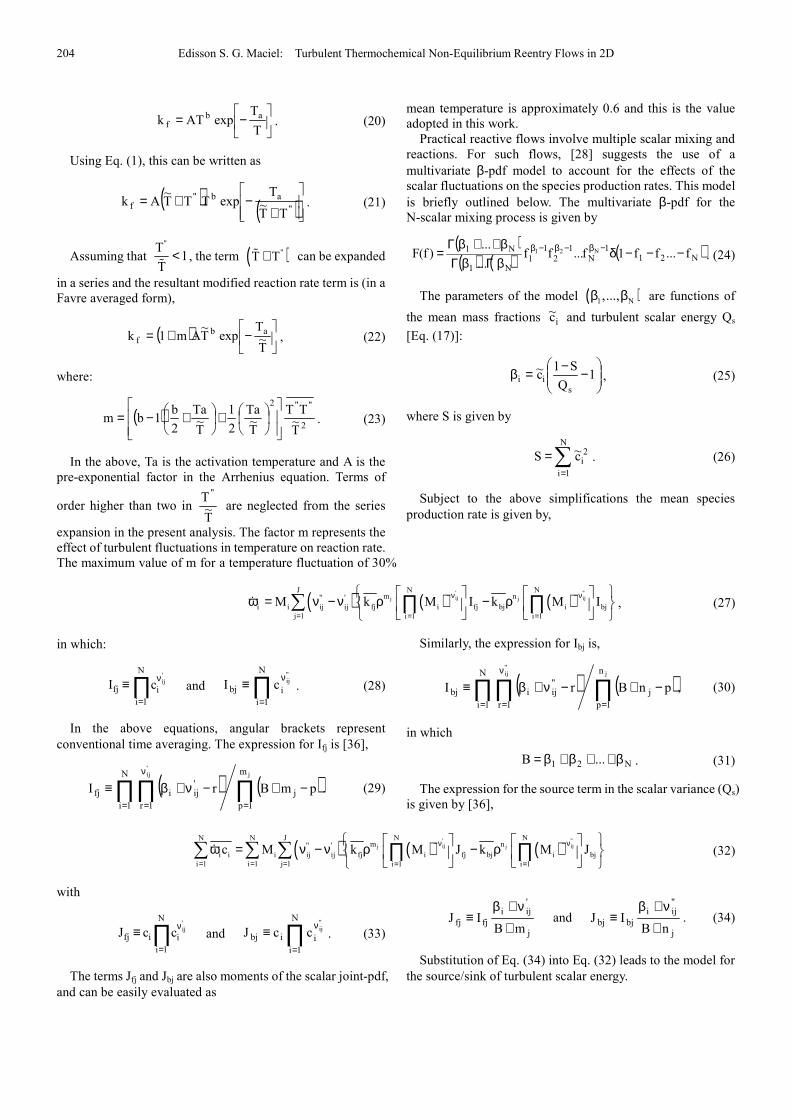
Practical reactive flows involve multiple scalar mixing and
reactions. For such flows, [28] suggests the use of a
multivariate β-pdf model to account for the effects of the
scalar fluctuations on the species production rates. This model
is briefly outlined below. The multivariate β-pdf for the
N-scalar mixing process is given by
( )( ) ( ) ( )N21
1
N1
2
1
1N1
N1 f...ff1f...ff...
...)f(F N21 −−−δ
βΓβΓβ++βΓ
= −β−β−β. (24)
The parameters of the model ( )1 N,...,β β are functions of
the mean mass fractions ic~ and turbulent scalar energy Qs
[Eq. (17)]:
−−=β 1
Q
S1c~
sii , (25)
where S is given by
∑=
=N
1i
2ic~S . (26)
Subject to the above simplifications the mean species
production rate is given by,
( ) ( ) ( )' "ij ijj j
N NJm n" '
i i ij ij fj i fj bj i bj
j 1 i 1 i 1
M k M I k M I−ν −ν
= = =
ω = ν − ν ρ − ρ
∑ ∏ ∏ɺ , (27)
in which:
∏=
ν≡N
1i
ifj
'ijcI and ∏
=
ν≡N
1i
ibj
"ijcI . (28)
In the above equations, angular brackets represent
conventional time averaging. The expression for Ifj is [36],
( ) ( )∏∏∏==
ν
=
−+−ν+β≡j
'ij m
1p
j
N
1i 1r
'ijifj pmBrI . (29)
Similarly, the expression for Ibj is,
( ) ( )∏∏∏==
ν
=
−+−ν+β≡j
"ij n
1p
j
N
1i 1r
"ijibj pnBrI , (30)
in which
N21 ...B β++β+β= . (31)
The expression for the source term in the scalar variance (Qs)
is given by [36],
( ) ( ) ( )' "ij ijj j
N NN N Jm n" '
i i i ij ij fj i fj bj i bj
i 1 i 1 j 1 i 1 i 1
c M k M J k M J−ν −ν
= = = = =
ω = ν − ν ρ − ρ
∑ ∑ ∑ ∏ ∏ɺ (32)
with
∏=
ν≡N
1i
iifj
'ijccJ and ∏
=
ν≡N
1i
iibj
"ijccJ . (33)
The terms Jfj and Jbj are also moments of the scalar joint-pdf,
and can be easily evaluated as
j
'iji
fjfjmB
IJ+
ν+β≡ and
j
"iji
bjbjnB
IJ+
ν+β≡ . (34)
Substitution of Eq. (34) into Eq. (32) leads to the model for
the source/sink of turbulent scalar energy.
Computational and Applied Mathematics Journal 2015; 1(4): 201-224 205
4. Navier-Stokes Equations
The flow is modelled by the Favre-averaged Navier-Stokes
equations and the condition of thermochemical
non-equilibrium, where the rotational and vibrational
contributions are considered, is taken into account. Only the
reactive Navier-Stokes equations for the five species model is
exhibited, although the seven species model could be obtained
including more two species equations and adjusting the
respective terms to this formulation. Details of the five species
model and seven species model implementation are described
in [21-24], and the interested reader is encouraged to read
these works to become aware of the present study.
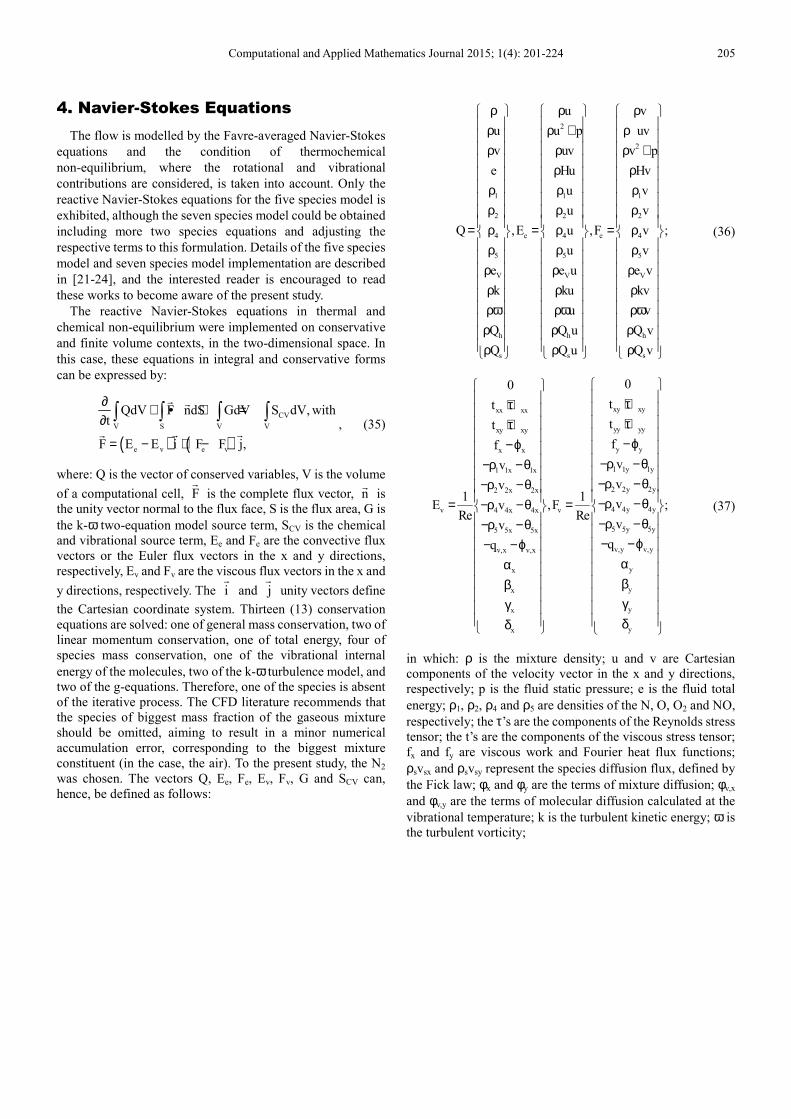
The reactive Navier-Stokes equations in thermal and
chemical non-equilibrium were implemented on conservative
and finite volume contexts, in the two-dimensional space. In
this case, these equations in integral and conservative forms
can be expressed by:
( ) ( )
CV
V S V V
e v e v
QdV F ndS GdV S dV, witht
F E E i F F j,
∂ + • + =∂
= − + −
∫ ∫ ∫ ∫� �
� ��, (35)
where: Q is the vector of conserved variables, V is the volume
of a computational cell, F�
is the complete flux vector, n�
is
the unity vector normal to the flux face, S is the flux area, G is
the k-ω two-equation model source term, SCV is the chemical
and vibrational source term, Ee and Fe are the convective flux
vectors or the Euler flux vectors in the x and y directions,
respectively, Ev and Fv are the viscous flux vectors in the x and
y directions, respectively. The i�
and j�
unity vectors define
the Cartesian coordinate system. Thirteen (13) conservation
equations are solved: one of general mass conservation, two of
linear momentum conservation, one of total energy, four of
species mass conservation, one of the vibrational internal
energy of the molecules, two of the k-ω turbulence model, and
two of the g-equations. Therefore, one of the species is absent
of the iterative process. The CFD literature recommends that
the species of biggest mass fraction of the gaseous mixture
should be omitted, aiming to result in a minor numerical
accumulation error, corresponding to the biggest mixture
constituent (in the case, the air). To the present study, the N2
was chosen. The vectors Q, Ee, Fe, Ev, Fv, G and SCV can,
hence, be defined as follows:
2
2
1 1 1
2 2 2
4 e 4 e 4
5 5 5
V V V
h h
s s
u v
u u p uv
v uv v p
e Hu Hv
u v
u v
Q ,E u ,F v
u v
e e u e v
k ku kv
u v
Q Q u
Q Q u
ρ ρ ρ ρ ρ + ρ ρ ρ ρ + ρ ρ ρ ρ ρ
ρ ρ ρ = ρ = ρ = ρ ρ ρ ρ
ρ ρ ρ ρ ρ ρ ρω ρω ρω ρ ρ ρ ρ ρ
h
s
;
Q v
Q v
ρ
(36)
xy xyxx xx
yy yyxy xy
y yx x
1 1y 1y1 1x 1x
2 2y 2y2 2x 2x
4 4y 4yv v4 4x 4x
5 5y 5y5 5x 5x
v,yv,x v,x
x
x
x
x
00
tt
tt
ff
vv
vv1 1
vE ,FvRe Re
vv
+τ+τ +τ+τ −ϕ−ϕ −ρ −θ−ρ −θ
−ρ −θ−ρ −θ −ρ −θ= =−ρ −θ −ρ −θ−ρ −θ
− −ϕ− −ϕ α β
γ δ
v,y
y
y
y
y
;
α β γ δ
(37)
in which: ρ is the mixture density; u and v are Cartesian
components of the velocity vector in the x and y directions,
respectively; p is the fluid static pressure; e is the fluid total
energy; ρ1, ρ2, ρ4 and ρ5 are densities of the N, O, O2 and NO,
respectively; the τ’s are the components of the Reynolds stress
tensor; the t’s are the components of the viscous stress tensor;
fx and fy are viscous work and Fourier heat flux functions;
ρsvsx and ρsvsy represent the species diffusion flux, defined by
the Fick law; φx and φy are the terms of mixture diffusion; φv,x
and φv,y are the terms of molecular diffusion calculated at the
vibrational temperature; k is the turbulent kinetic energy; ω is
the turbulent vorticity;
206 Edisson S. G. Maciel: Turbulent Thermochemical Non-Equilibrium Reentry Flows in 2D
( )
1
2
4CV
5
*
s v,s v,s s s v,s
s mol s mol
0
0
0
0
S ;
e e e
0
0
0
0
= =
ω
ω ω=
ω
ρ − τ + ω
∑ ∑
ɺ
ɺ
ɺ
ɺ
ɺ
(38)
k
22
T
T
22
T T T
T
0
0
0
0
0
0
0
0G
0
G
G
2 h h
Re Pr d x y
2 c c
ReSc x y Re
ω
=
µ ∂ ∂ + ∂ ∂ µ ∂ ∂ Ψ + + ∂ ∂
. (39)
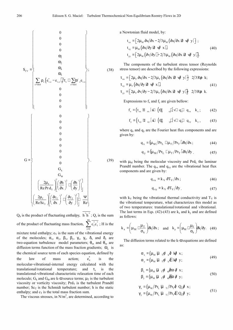
Qh is the product of fluctuating enthalpy, ""hh ; Qs is the sum
of the product of fluctuating mass fraction, ∑=
ns
1i
"i
"i cc ; H is the
mixture total enthalpy; eV is the sum of the vibrational energy
of the molecules; αx, αy, βx, βy, γx, γy, δx and δy are
two-equation turbulence model parameters; θsx and θsy are
diffusion terms function of the mass fraction gradients; sωɺ is
the chemical source term of each species equation, defined by
the law of mass action; *ve is the
molecular-vibrational-internal energy calculated with the
translational/rotational temperature; and τs is the
translational-vibrational characteristic relaxation time of each
molecule; Gk and Gω are k-ω source terms; µT is the turbulent
viscosity or vorticity viscosity; PrdT is the turbulent Prandtl
number; ScT is the Schmidt turbulent number; h is the static
enthalpy; and cT is the total mass fraction sum.
The viscous stresses, in N/m2, are determined, according to
a Newtonian fluid model, by:
( )( )
( ) ( )
xx M M
xy M
yy M M
t 2 u x 2 3 u x v y ;
t u y v x ;
t 2 v y 2 3 u x v y .
= µ ∂ ∂ − µ ∂ ∂ + ∂ ∂
= µ ∂ ∂ + ∂ ∂
= µ ∂ ∂ − µ ∂ ∂ + ∂ ∂
(40)
The components of the turbulent stress tensor (Reynolds
stress tensor) are described by the following expressions:
( )( )
( )
xx T T
xy T
yy T T
2 u x 2 3 u x v y 2 3Re k;
u y v x ;
2 v y 2 3 u x v y 2 3Re k.
τ = µ ∂ ∂ − µ ∂ ∂ + ∂ ∂ − ρ
τ = µ ∂ ∂ + ∂ ∂
τ = µ ∂ ∂ − µ ∂ ∂ + ∂ ∂ − ρ
(41)
Expressions to fx and fy are given bellow:
( ) ( )x xx xx xy xy x vx xf t u t v q q k= + τ + + τ + + + ; (42)
( ) ( )y xy xy yy yy y vy yf t u t v q q k= + τ + + τ + + + , (43)
where qx and qy are the Fourier heat flux components and are
given by:
( ) ;xhPrPrq TTLMx ∂∂µ+µ= (44)
( ) yhPrPrq TTLMy ∂∂µ+µ= . (45)
with µM being the molecular viscosity and PrdL the laminar
Prandtl number. The qvx and qvy are the vibrational heat flux
components and are given by:
;xTkq VVvx ∂∂= (46)
yTkq VVvy ∂∂= . (47)
with kV being the vibrational thermal conductivity and TV is
the vibrational temperature, what characterizes this model as
of two temperatures: translational/rotational and vibrational.
The last terms in Eqs. (42)-(43) are kx and ky and are defined
as follows:
;xkkk
TMx ∂∂
σµ
+µ= and .ykkk
TMy ∂∂
σµ+µ= (48)
The diffusion terms related to the k-ω equations are defined
as:
( )( )
x M T k
y M T k
k x;
k y;
α = µ + µ σ ∂ ∂
α = µ + µ σ ∂ ∂ (49)
( )( )
x M T
y M T
x;
y;
ω
ω
β = µ + µ σ ∂ω ∂
β = µ + µ σ ∂ω ∂ (50)
( )( )
x M L T T h
y M L T T h
Pr Pr Q x;
Pr Pr Q y;
γ = µ + µ ∂ ∂
γ = µ + µ ∂ ∂ (51)
Computational and Applied Mathematics Journal 2015; 1(4): 201-224 207
( )( )
x M T T S
y M T T S
Sc Sc Q x;
Sc Sc Q y;
δ = µ + µ ∂ ∂
δ = µ + µ ∂ ∂ (52)
The terms of species diffusion, defined by the Fick law, to a
condition of thermal non-equilibrium, are determined by
([29]):
x
YDv
s,MFssxs ∂
∂ρ−=ρ and
y
YDv
s,MFssys ∂
∂ρ−=ρ , (53)
with “s” referent to a given species, YMF,s being the molar
fraction of the species, defined as:
∑=
ρ
ρ=
ns
1k
kk
sss,MF
M
MY
(54)
and Ds is the species-effective-diffusion coefficient.
The diffusion terms φx and φy which appear in the energy
equation are defined by ([16]):
∑=
ρ=φns
1s
ssxsx hv and ∑=
ρ=φns
1s
ssysy hv , (55)
being hs the specific enthalpy (sensible) of the chemical
species “s”. The molecular diffusion terms calculated at the
vibrational temperature, φv,x and φv,y, which appear in the
vibrational-internal-energy equation are defined by ([29]):
∑=
ρ=φmols
s,vsxsx,v hvand ∑
=
ρ=φmols
s,vsysy,v hv, (56)
with hv,s being the specific enthalpy (sensible) of the chemical
species “s” calculated at the vibrational temperature TV. The
sum of Eq. (56), as also those present in Eq. (38), considers
only the molecules of the system, namely: N2, O2 and NO.
Finally, the θ’s terms of Eq. (37) are described as,
( ) ;xcScSc STTMsx ∂∂µ+µ=θ (57)
( ) ycScSc STTMsy ∂∂µ+µ=θ . (58)
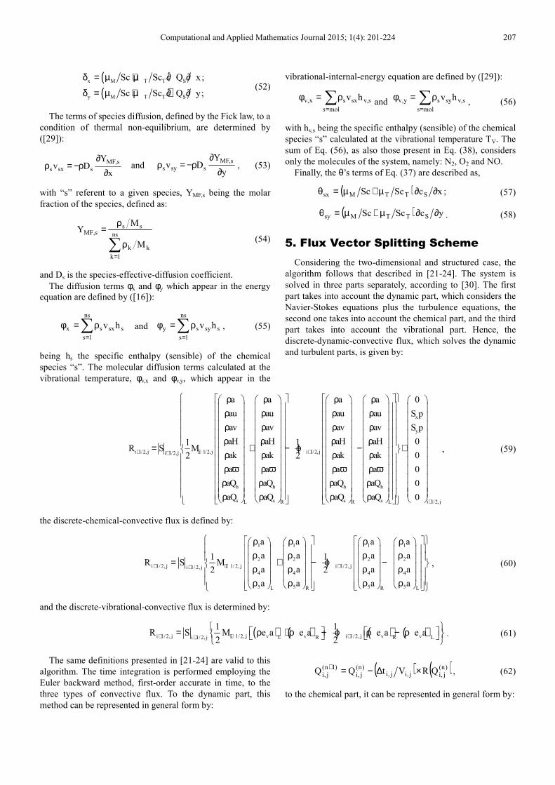
5. Flux Vector Splitting Scheme
Considering the two-dimensional and structured case, the
algorithm follows that described in [21-24]. The system is
solved in three parts separately, according to [30]. The first
part takes into account the dynamic part, which considers the
Navier-Stokes equations plus the turbulence equations, the
second one takes into account the chemical part, and the third
part takes into account the vibrational part. Hence, the
discrete-dynamic-convective flux, which solves the dynamic
and turbulent parts, is given by:
i 1/2, j i 1/2,j i 1/2, ji 1/2,j
h h
s sL R
a a a
au au au
av av av
aH aH aH1 1R S M
ak ak ak2 2
a a a
aQ aQ
aQ aQ
+ + ++
ρ ρ ρ ρ ρ ρ ρ ρ ρ
ρ ρ ρ = + − ϕ ρ ρ ρ ρ ω ρ ω ρ ω ρ ρ ρ
ρ ρ
x
y
h h
s s i 1/2, jR L
a 0
au S p
av S p
aH 0
ak 0
a 0
aQ aQ 0
aQ aQ 0 +
ρ ρ ρ
ρ − + ρ ρ ω ρ ρ ρ
, (59)
the discrete-chemical-convective flux is defined by:
1 1 1 1
2 2 2 2
i 1/2, j i 1/ 2, j i 1/2, ji 1/2, j4 4 4 4
5 5 5 5L R R L
a a a a
a a a a1 1R S M
a a a a2 2
a a a a
+ + ++
ρ ρ ρ ρ ρ ρ ρ ρ = + − ϕ − ρ ρ ρ ρ ρ ρ ρ ρ
, (60)
and the discrete-vibrational-convective flux is determined by:
( ) ( ) ( ) ( )i 1/2, j i 1/2, j v v i 1/2, j v vL R R Li 1/ 2, j
1 1R S M e a e a e a e a
2 2+ + ++
= ρ + ρ − ϕ ρ − ρ
. (61)
The same definitions presented in [21-24] are valid to this
algorithm. The time integration is performed employing the
Euler backward method, first-order accurate in time, to the
three types of convective flux. To the dynamic part, this
method can be represented in general form by:
( ) ( ))n(
j,ij,ij,i)n(
j,i
)1n(
j,iQRVtQQ ×∆−=+
, (62)
to the chemical part, it can be represented in general form by:
208 Edisson S. G. Maciel: Turbulent Thermochemical Non-Equilibrium Reentry Flows in 2D
( ) ( )[ ])n(
j,iCj,i)n(
j,ij,i)n(
j,i
)1n(
j,iQSVQRtQQ −×∆−=+
, (63)
where the chemical source term SC is calculated with the
temperature Trrc (reaction rate controlling temperature).
Finally, to the vibrational part:
( ) ( )[ ])n(
j,ivj,i)n(
j,ij,i)n(
j,i
)1n(
j,iQSVQRtQQ −×∆−=+
, (64)
in which:
∑∑==
− +=mols
s,vs,C
mols
s,VTv eSqS, (65)
where qT-V is the heat flux due to translational-vibrational
relaxation, defined in [21-24].
The definition of the dissipation term φ determines the
particular formulation of the convective fluxes. The choice
below corresponds to the [13] scheme, according to [31]:
( )( )
i 1/2,j i 1/2,j
2VL
i 1/2,j i 1/2,j i 1/2,j R i 1/2,j
2
i 1/2,j L i 1/2,j
M , if M 1;
M 0.5 M 1 , if 0 M 1;
M 0.5 M 1 , if 1 M 0.
+ +
+ + + +
+ +
≥ϕ =ϕ = + − ≤ < + + − < ≤
(66)
This scheme is first-order accurate in space and in time. The
high-order spatial accuracy is obtained, in this study, by the
ENO procedure..
The viscous formulation follows that of [32], which adopts
the Green theorem to calculate primitive variable gradients.
The viscous vectors are obtained by arithmetical average
between cell (i,j) and its neighbors. As was done with the
convective terms, there is a need to separate the viscous flux in
three parts: dynamical viscous flux, chemical viscous flux and
vibrational viscous flux. The dynamical part corresponds to
the first four equations of the Navier-Stokes ones plus the four
equations of the turbulence model, the chemical part
corresponds to the four equations immediately below the
energy equation and the vibrational part corresponds to the
equation below the last chemical species one.
6. ENO Procedure
ENO schemes overcome the limitations of TVD schemes
by relaxing the requirement of total variation non-increasing
([33]). They are conservative, essentially non-oscillatory and
give uniform accuracy in smooth regions, without the
degradation of accuracy at non-sonic local extrema as
observed with TVD methods. There are several possible
approaches when constructing ENO schemes. [9] use the ENO
scheme to construct a higher order solution to the cell-average
of the conservation equation using a sliding average. The ENO
scheme of [9], therefore, gives an r-th order accurate
approximation to the cell averages. According to [9], the ENO
schemes can be expressed as:
)Q(cRe)(EAQ)(E hh •τ•≡•τ , (67)
where:
Q)(Eh •τ is the new ENO scheme applied to the cell
average solution;
hA is the cell averaging operator;
)(E τ is the exact evolution operator (the solver);
)Q(cRe is the reconstruction operator;
Q is the average solution.
The most important ingredient of their ENO method is the
reconstruction of the point values Q(x,y) from the cell
averaged values j,iQ . These point values are necessary to
compute the flux at the cell faces. This is done with a
reconstruction method that is conservative, essentially
non-oscillatory and gives at all points in a neighborhood
around (xi,yi) an r-th order approximation to Q, when Q is
smooth. This formulation is employed in the present work.
The implementation of the ENO method of [9] in the [13]
scheme, where the ENO method uses a reconstruction from
the cell averaged variables, is straightforward. The first step in
the ENO reconstruction is the determination of the cell
averaged variables. In the present work, it was adopted that the
averaged operator is the identity operator; hence, the averaged
variables are exactly the conserved variable at the cell point. A
higher order polynomial representation of Q in each cell is
now constructing by determining the divided differences used
in the Newton interpolation method using the following
recursive algorithm: Considering the ξ direction, the divided
differences are calculated as follows:
0 i, j i, j i, j 1 i 1, j i 1, j i 1, jH [ ] Q( ) Q ;H [ ] Q( ) Q ;+ + +ξ = ξ = ξ = ξ = (68)
[ ] ( )j,ij,1ij,i0j,1i1j,1ij,i00 )(H)(H],[H ξ−ξξ−ξ=ξξ +++ ; (69)
{ } ( )000 01 00i, j i 1, j i 2, j i 1, j i 2, j i, j i 1, j i 2, j i, jH [ , , ] H , H ,+ + + + + + ξ ξ ξ = ξ ξ − ξ ξ ξ − ξ ; (70)
If the divided difference ],,[H j,2ij,1ij,i000 ++ ξξξ is larger
than ],,[H j,3ij,2ij,1i001 +++ ξξξ choose ],,[HH j,3ij,2ij,1i001000 +++ ξξξ= ;
otherwise, ],,[H j,2ij,1ij,i000 ++ ξξξ is accepted. This process
is repeated until the required order of the interpolation is
obtained and applied to each component of Q independently.
Note that the calculated stencil is computed dynamically at
each point and is non-linear in nature. With the choice of the
minimum divided difference at a point, the best molecule is
determined to provide high accuracy.
Computational and Applied Mathematics Journal 2015; 1(4): 201-224 209
After the determination of the coefficients of the Newton polynomial, the reconstruction process is finished:
i, j 0 i, j 00 i, j i 1, j 000 i, j i 1, j i 2, jRec( ,Q) Q( ) H ( ) H ( )( ) H ( )( )( ) ...+ + +ξ = ξ + ξ − ξ + ξ − ξ ξ − ξ + ξ − ξ ξ − ξ ξ − ξ + (71)
This process gives a representation of the solution in each
cell and can be used to determine the values of Q at the cell
faces. The values at the left and right side of the cell, as in the
MUSCL (Monotone Upstream-centered Schemes for
Conservation Laws) case, are now used in the [13] solver,
which gives the fluxes Ri+1/2,j. Observe that the reconstruction
process results in a polynomial of order r-th to the vector of
conserved variables as function of the generalized coordinate
ξ. The same reasoning is applied to the η direction.
7. Turbulence Models
7.1. Coakley Turbulence Model
The [4] model is a k1/2
-ω one. The turbulent Reynolds
number is defined as
MNkR ν= . (72)
The production term of turbulent kinetic energy is given by
Rey
u
x
v
y
uP
∂∂
∂∂+
∂∂= . (73)
The function χ is defined as
1PC 2 −ω=χ µ . (74)
The damping function is given by
βχ+−=
α−
1
e1D
R
. (75)
The turbulent viscosity is defined by
ωρ=µ µ kDCReT , (76)
with: Cµ a constant to be defined.
To the [4] model, the Gk and Gω terms have the following
expressions:
kkk DPG −−= and ωωω −−= DPG , (77)
where:
k k2
0.5C DP 2 u vP k Re;D 0.5 1 k Re;
x y3
µ ∂ ∂= ρω = − + ω− ρω ∂ ∂ω (78)
( )2 2 2
1 1 2
2 u vP CC P Re;D C C Re,
x y3ω µ ω
∂ ∂= ω ρω = − + ω− ρω ∂ ∂ (79)
where 045.0D405.0C1 += . The closure coefficients
adopted for the [4] model are: 0.1k =σ ; 3.1=σω ;
09.0C =µ ; 92.0C2 = ; 5.0=β ; 0065.0=α ; PrdL = 0.72;
PrdT = 0.9.
7.2. Wilcox Turbulence Model
The turbulent viscosity is expressed in terms of k and ω as:
ωρ=µ kReT . (80)
In this model, the quantities kσ and ωσ have the values
*1 σ and σ1 , respectively, where *σ and σ are model
constants.
To the [5] model, the Gk and Gω terms have the following
expressions:
kkk DPG +−= and ωωω +−= DPG , (81)
where:
Rey
u
x
v
y
uP Tk ∂
∂
∂∂+
∂∂µ= and RekD *
k ωρβ= ; (82)
kPk
P
αω=ω and ReD 2ωβρ=ω , (83)
where the closure coefficients adopted for the [5] model are:
09.0* =β ; 403=β ; 5.0* =σ ; 5.0=σ ; 95=α ; PrdL =
0.72; PrdT = 0.9.
7.3. Yoder, Georgiadids, and Orkwis
Turbulence Model
The turbulent Reynolds number is specified by:
( )ωµρ= MT /kRe . (84)
The parameter α* is given by:
( ) ( )kTkT*0
* RRe1RRe ++α=α . (85)
The turbulent viscosity is specified by:
ωρα=µ /kRe *T . (86)
The source term denoted by G in the governing equation
210 Edisson S. G. Maciel: Turbulent Thermochemical Non-Equilibrium Reentry Flows in 2D
contains the production and dissipation terms of k and ω. To
the [6] model, the Gk and ωG terms have the following
expressions:
kkk DPG +−= and ωωω +−= DPG . (87)
To define the production and dissipation terms, it is
necessary to define firstly some parameters. The turbulent
Mach number is defined as:
2T a/k2M = . (88)
It is also necessary to specify the function F:
( )0.0,MMMAXF2
0,T2T −= . (89)
The *β parameter is given by:
( )[ ] ( )[ ]4ST
4ST
* R/Re1R/Re18/509.0 ++=β (90)
Finally, the production and dissipation terms of Eq. (87) are
given by
( )*
k T k k
u v uP ;D k 1 F / Re;
y x y
∂ ∂ ∂= µ + = β ρω + ξ ∂ ∂ ∂ (91)
kkP/P αω=ω ; and ( ) ReFD*2
ωω ξβ+βρω= , (92)
with:
( )( ) *TT0 RRe1RRe9/5 α++α=α ωω . (93)
The [6] turbulence model adopts the following closure
coefficients: Rs = 8.0, Rk = 6.0, Rω = 2.7, ξk = 1.0, ξω = 0.0, β =
3/40, MT,0 = 0.0, α0 = 0.1, 3/*0 β=α , 0.2k =σ and
0.2=σω .
8. Physical Problem and Mesh
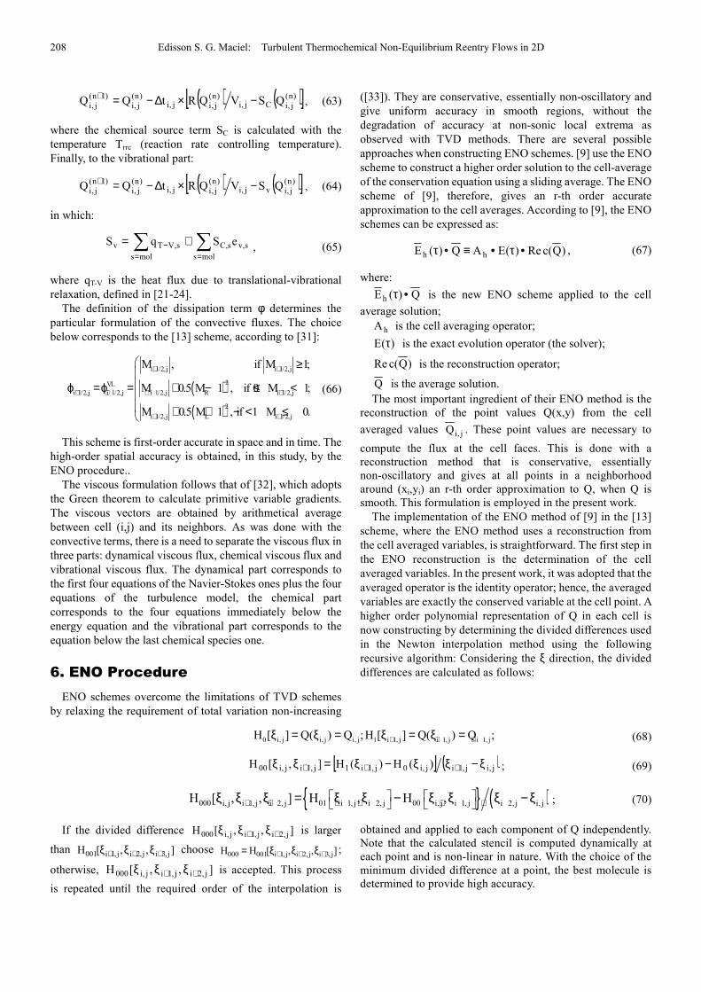
Figure 1. Blunt body viscous mesh.
One physical problem is studied in this work: the blunt body
problem. The geometry under study is a blunt body with 1.0 m
of nose ratio and parallel rectilinear walls. The far field is
located at 20.0 times the nose ratio in relation to the
configuration nose.
Figures 1 shows the viscous mesh used to the blunt body
problem. This mesh is composed of 2,548 rectangular cells
and 2,650 nodes, employing an exponential stretching of 5.0%.
This mesh is equivalent in finite differences to a one of 53x50
points. A “O” type mesh is taken as the base to construct such
mesh. No smoothing is used in this mesh generation process,
being this one constructed in Cartesian coordinates.
9. Results
Tests were performed in a Core i7 processor of 2.1GHz and
8.0Gbytes of RAM microcomputer, in a Windows 8.0
environment. Four (4) orders of reduction of the maximum
residual in the field were considered to obtain a converged
solution; however, with the minimum of three (3) orders the
author considered the solution converged. The residual was
defined as the value of the discretized conservation equation.
The entrance or attack angle was adopted equal to zero.
The initial conditions to this problem, for a five species
chemical model, are presented in Tab. 1. To the seven species
chemical model, the unique difference is the inclusion of
+NOc and −e
c with values equal to zero. LREF is the
reference length, equal to L in the present study. The boundary
conditions are described in [34]. The interested reader is
encouraged to read this reference to become familiar with the
present implementation. Reynolds number is obtained from
[35].
Table 1. Initial conditions to the problem of the blunt body.
Property Value
M∞ 8.78
ρ∞ 0.00326 kg/m3
p∞ 687 Pa
U∞ 4,776 m/s
T∞ 694 K
Tv,∞ 694 K
Altitude 40,000 m
cN 10-9
cO 0.07955
2Oc
0.13400
cNO 0.05090
L 2.0 m
Re∞ 2.3885x10⁶
k∞ 10-6
ω∞ 10u/LREF
Qh 10-4h∞
Qs 10-2∑=
∞
N
si
2,sc
9.1. Coakley Results
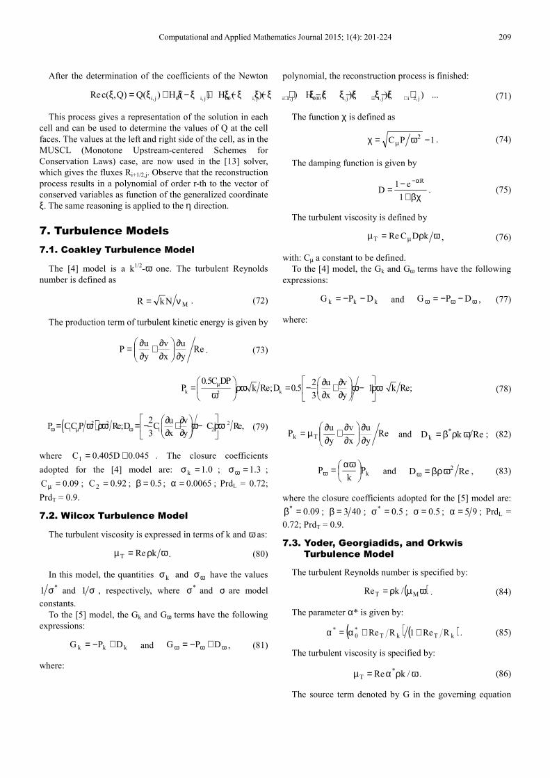
5 Species Model. Figure 2 shows the pressure contours
obtained by the [13] scheme as using the [4] turbulence model.
Computational and Applied Mathematics Journal 2015; 1(4): 201-224 211
The value of the pressure peak is around 186.37 unities. Good
symmetry properties are observed. The normal shock wave is
well captured by the numerical algorithm.
Figure 2. Pressure contours (C).
Figure 3. Mach number contours (C).
Figure 3 exhibits the Mach number contours generated by
the [13] numerical scheme as using the [4] turbulence model.
Some pre-shock oscillations appear close to the oblique part of
the shock wave. Although the Mach number peak is not
significantly higher than the initial condition, it is suffice to
generate pre-shock oscillations. Good symmetry properties
are observed. The subsonic region behind the normal part of
the shock wave is well captured.
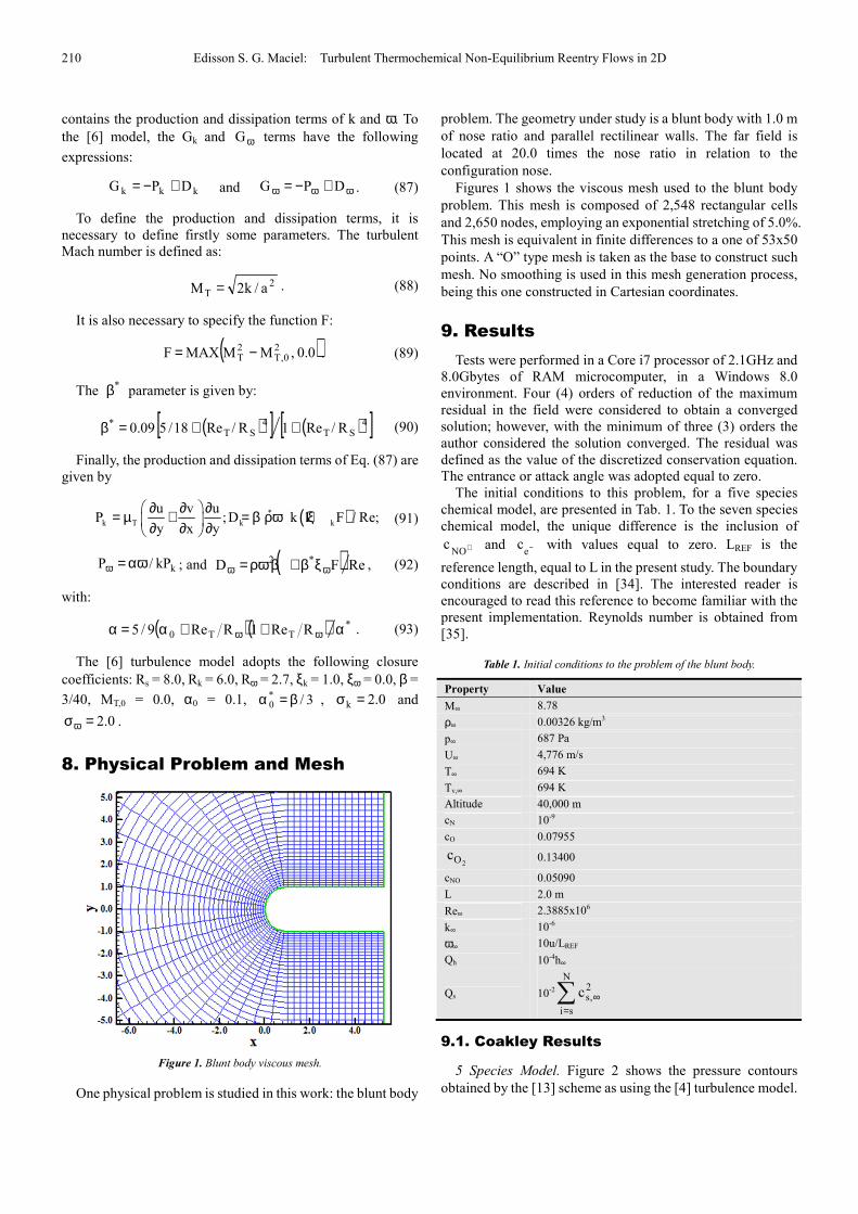
Figure 4 presents the translational/rotational temperature
contours obtained by the [13] numerical scheme as using the
[4] turbulence model. A region of intense energy exchange is
observed close to the body’s wall. The heat conduction along
the body is well captured by the numerical scheme. Good
symmetry properties are observed. The temperature peak is
around 8,742.67 K, which agrees with standard values
computed to this simulation (see [36]).
Figure 4. Translational/rotational temperature contours (C).
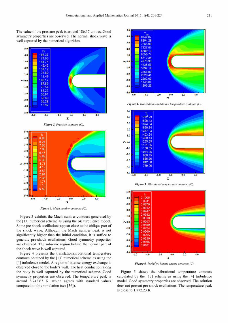
Figure 5. Vibrational temperature contours (C).
Figure 6. Turbulent kinetic energy contours (C).
Figure 5 shows the vibrational temperature contours
calculated by the [13] scheme as using the [4] turbulence
model. Good symmetry properties are observed. The solution
does not present pre-shock oscillations. The temperature peak
is close to 1,772.23 K.
212 Edisson S. G. Maciel: Turbulent Thermochemical Non-Equilibrium Reentry Flows in 2D
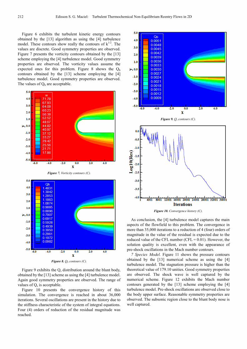
Figure 6 exhibits the turbulent kinetic energy contours
obtained by the [13] algorithm as using the [4] turbulence
model. These contours show really the contours of k1/2
. The
values are discrete. Good symmetry properties are observed.
Figure 7 presents the vorticity contours obtained by the [13]
scheme employing the [4] turbulence model. Good symmetry
properties are observed. The vorticity values assume the
expected ones for this problem. Figure 8 shows the Qh
contours obtained by the [13] scheme employing the [4]
turbulence model. Good symmetry properties are observed.
The values of Qh are acceptable.
Figure 7. Vorticity contours (C).
Figure 8. Qh contours (C).
Figure 9 exhibits the Qs distribution around the blunt body,
obtained by the [13] scheme as using the [4] turbulence model.
Again good symmetry properties are observed. The range of
values of Qs is acceptable.
Figure 10 presents the convergence history of this
simulation. The convergence is reached in about 36,000
iterations. Several oscillations are present in the history due to
the stiffness characteristic of the system of integral equations.
Four (4) orders of reduction of the residual magnitude was
reached.
Figure 9. Qs contours (C).
Figure 10. Convergence history (C).
As conclusion, the [4] turbulence model captures the main
aspects of the flowfield to this problem. The convergence in
more than 35,000 iterations to a reduction of 4 (four) orders of
magnitude in the value of the residual is expected due to the
reduced value of the CFL number (CFL = 0.01). However, the
solution quality is excellent, even with the appearance of
pre-shock oscillations in the Mach number contours.
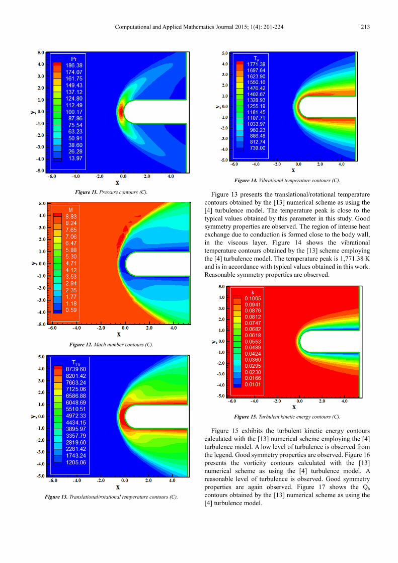
7 Species Model. Figure 11 shows the pressure contours
obtained by the [13] numerical scheme as using the [4]
turbulence model. The stagnation pressure is higher than the
theoretical value of 179.10 unities. Good symmetry properties
are observed. The shock wave is well captured by the
numerical scheme. Figure 12 exhibits the Mach number
contours generated by the [13] scheme employing the [4]
turbulence model. Pre-shock oscillations are observed close to
the body upper surface. Reasonable symmetry properties are
observed. The subsonic region close to the blunt body nose is
well captured.
Computational and Applied Mathematics Journal 2015; 1(4): 201-224 213
Figure 11. Pressure contours (C).
Figure 12. Mach number contours (C).
Figure 13. Translational/rotational temperature contours (C).
Figure 14. Vibrational temperature contours (C).
Figure 13 presents the translational/rotational temperature
contours obtained by the [13] numerical scheme as using the
[4] turbulence model. The temperature peak is close to the
typical values obtained by this parameter in this study. Good
symmetry properties are observed. The region of intense heat
exchange due to conduction is formed close to the body wall,
in the viscous layer. Figure 14 shows the vibrational
temperature contours obtained by the [13] scheme employing
the [4] turbulence model. The temperature peak is 1,771.38 K
and is in accordance with typical values obtained in this work.
Reasonable symmetry properties are observed.
Figure 15. Turbulent kinetic energy contours (C).
Figure 15 exhibits the turbulent kinetic energy contours
calculated with the [13] numerical scheme employing the [4]
turbulence model. A low level of turbulence is observed from
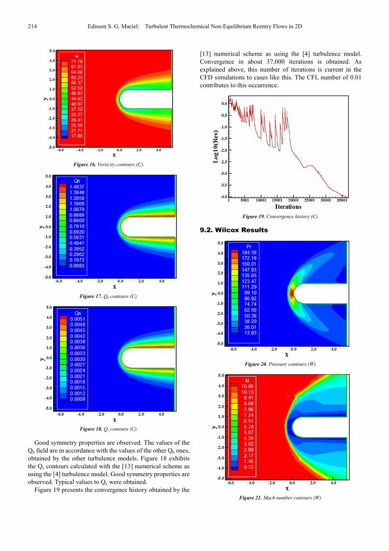
the legend. Good symmetry properties are observed. Figure 16
presents the vorticity contours calculated with the [13]
numerical scheme as using the [4] turbulence model. A
reasonable level of turbulence is observed. Good symmetry
properties are again observed. Figure 17 shows the Qh
contours obtained by the [13] numerical scheme as using the
[4] turbulence model.
214 Edisson S. G. Maciel: Turbulent Thermochemical Non-Equilibrium Reentry Flows in 2D
Figure 16. Vorticity contours (C).
Figure 17. Qh contours (C).
Figure 18. Qs contours (C).
Good symmetry properties are observed. The values of the
Qh field are in accordance with the values of the other Qh ones,
obtained by the other turbulence models. Figure 18 exhibits
the Qs contours calculated with the [13] numerical scheme as
using the [4] turbulence model. Good symmetry properties are
observed. Typical values to Qs were obtained.
Figure 19 presents the convergence history obtained by the
[13] numerical scheme as using the [4] turbulence model.
Convergence in about 37,000 iterations is obtained. As
explained above, this number of iterations is current in the
CFD simulations to cases like this. The CFL number of 0.01
contributes to this occurrence.
Figure 19. Convergence history (C).
9.2. Wilcox Results
Figure 20. Pressure contours (W).
Figure 21. Mach number contours (W).
Computational and Applied Mathematics Journal 2015; 1(4): 201-224 215
5 Species Model. Figure 20 shows the pressure contours
obtained by the [13] numerical scheme as using the [5]
turbulence model. Good symmetry properties are observed.
The stagnation pressure predicted by this turbulence model is
closer to the theoretical value than the [4] one.
Figure 21 exhibits the Mach number contours generated by
the [13] numerical algorithm as using the [5] turbulence model.
The contours are free of pre-shock oscillations, although high
values of Mach number were obtained. Good symmetry
characteristics are observed. The subsonic region behind the
normal shock portion of the shock wave is well captured.
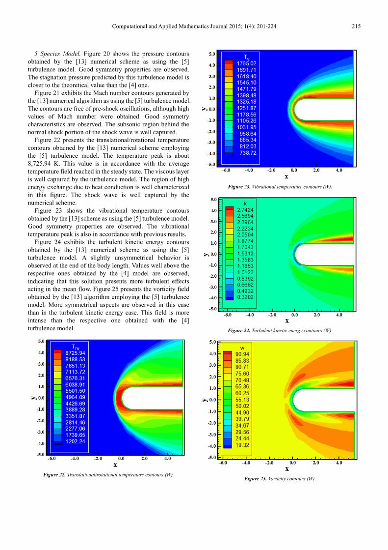
Figure 22 presents the translational/rotational temperature
contours obtained by the [13] numerical scheme employing
the [5] turbulence model. The temperature peak is about
8,725.94 K. This value is in accordance with the average
temperature field reached in the steady state. The viscous layer
is well captured by the turbulence model. The region of high
energy exchange due to heat conduction is well characterized
in this figure. The shock wave is well captured by the
numerical scheme.
Figure 23 shows the vibrational temperature contours
obtained by the [13] scheme as using the [5] turbulence model.
Good symmetry properties are observed. The vibrational
temperature peak is also in accordance with previous results.
Figure 24 exhibits the turbulent kinetic energy contours
obtained by the [13] numerical scheme as using the [5]
turbulence model. A slightly unsymmetrical behavior is
observed at the end of the body length. Values well above the
respective ones obtained by the [4] model are observed,
indicating that this solution presents more turbulent effects
acting in the mean flow. Figure 25 presents the vorticity field
obtained by the [13] algorithm employing the [5] turbulence
model. More symmetrical aspects are observed in this case
than in the turbulent kinetic energy case. This field is more
intense than the respective one obtained with the [4]
turbulence model.
Figure 22. Translational/rotational temperature contours (W).
Figure 23. Vibrational temperature contours (W).
Figure 24. Turbulent kinetic energy contours (W).
Figure 25. Vorticity contours (W).
216 Edisson S. G. Maciel: Turbulent Thermochemical Non-Equilibrium Reentry Flows in 2D
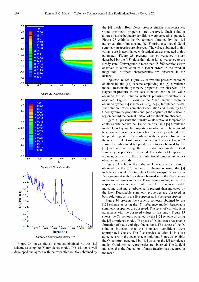
Figure 26. Qh contours (W).
Figure 27. Qs contours (W).
Figure 28. Convergence history (W).
Figure 26 shows the Qh contours obtained by the [13]
scheme as using the [5] turbulence model. The solution is well
developed and agrees with the respective solution obtained by
the [4] model. Both fields present similar characteristics.
Good symmetry properties are observed. Such solution
assures that the boundary conditions were correctly stipulated.
Figure 27 exhibits the Qs contours obtained by the [13]
numerical algorithm as using the [5] turbulence model. Good
symmetry properties are observed. The values obtained to this
variable are in accordance with typical values expected to this
parameter. Figure 28 presents the convergence history
described by the [13] algorithm along its convergence to the
steady state. Convergence in more than 45,500 iterations were
observed to a reduction of 4 (four) orders in the residual
magnitude. Stiffness characteristics are observed in the
history.
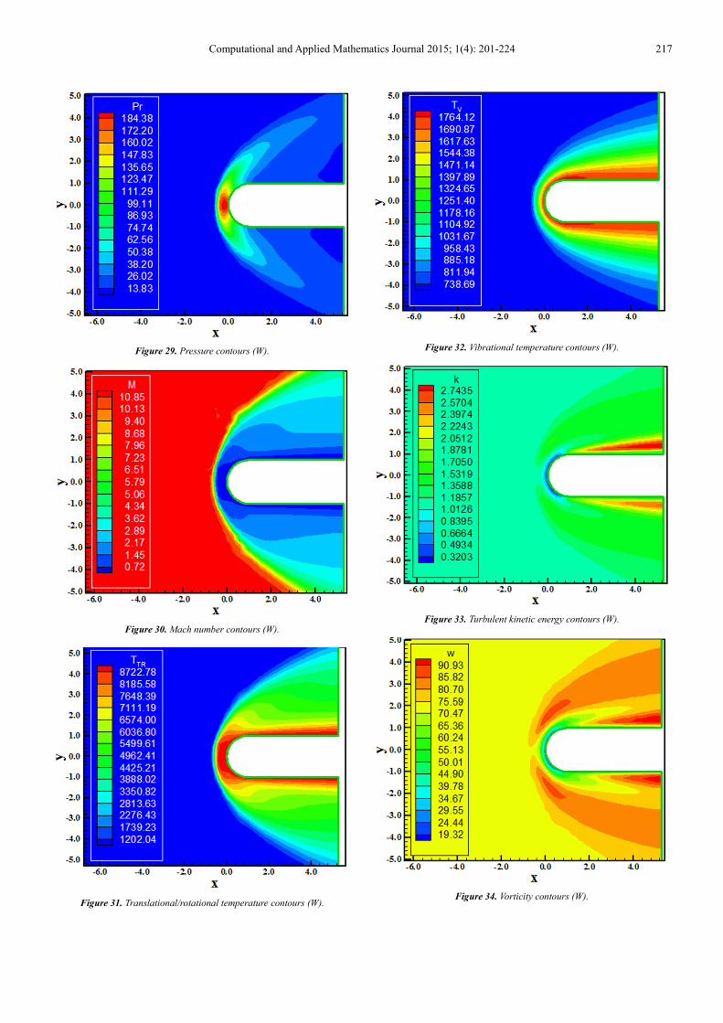
7 Species Model. Figure 29 shows the pressure contours
obtained by the [13] scheme employing the [5] turbulence
model. Reasonable symmetry properties are observed. The
stagnation pressure in this case is better than the last value
obtained for it. Solution without pressure oscillations is
observed. Figure 30 exhibits the Mach number contours
obtained by the [13] scheme as using the [5] turbulence model.
The solution presents pre-shock oscillation and instability free.
Good symmetry properties and good capture of the subsonic
region behind the normal portion of the shock are observed.
Figure 31 presents the translational/rotational temperature
contours obtained by the [13] scheme as using [5] turbulence
model. Good symmetry properties are observed. The region of
heat conduction in the viscous layer is clearly captured. The
temperature peak is in accordance with the peaks observed in
the other turbulent solutions presented in this work. Figure 32
shows the vibrational temperature contours obtained by the
[13] scheme as using the [5] turbulence model. Good
symmetry properties are observed. The values of temperature
are in agreement with the other vibrational temperature values
observed in this study.
Figure 33 exhibits the turbulent kinetic energy contours
obtained by the [13] numerical scheme as using the [5]
turbulence model. The turbulent kinetic energy values are in
fair agreement with the values obtained with the five species
model to the same simulation. These values are higher than the
respective ones obtained with the [4] turbulence model,
indicating that more turbulence is present than indicated by
the later. Reasonable symmetry properties are observed in
both solutions, as in the five species as in the seven species.
Figure 34 presents the vorticity contours obtained by the
[13] scheme as using the [5] turbulence model. Reasonable
symmetry properties are observed. The level of vorticity is in
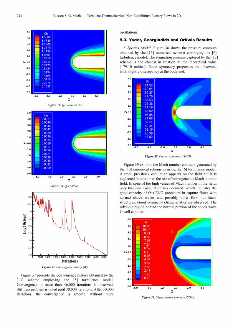
agreement with the observed values in this study. Figure 35
shows the Qh contours obtained by the [13] scheme as using
the [5] turbulence model. The peak of Qh indicates reasonable
formation of static enthalpy fluctuations. The aspect of the Qh
solution indicates that the boundary conditions were
appropriated chosen. The five species solution is in close
agreement with the seven species solution. Figure 36 exhibits
the Qs contours generated by [13] as using the [5] turbulence
model. Good symmetry properties are observed. The Qs field
indicates that the fluctuation of mass fraction has occurred in
the mean.
Computational and Applied Mathematics Journal 2015; 1(4): 201-224 217
Figure 29. Pressure contours (W).
Figure 30. Mach number contours (W).
Figure 31. Translational/rotational temperature contours (W).
Figure 32. Vibrational temperature contours (W).
Figure 33. Turbulent kinetic energy contours (W).
Figure 34. Vorticity contours (W).
218 Edisson S. G. Maciel: Turbulent Thermochemical Non-Equilibrium Reentry Flows in 2D
Figure 35. Qh contours (W).
Figure 36. Qs contours.
Figure 37. Convergence history (W).
Figure 37 presents the convergence history obtained by the
[13] scheme employing the [5] turbulence model.
Convergence in more than 46,000 iterations is observed.
Stiffness problem is noted until 30,000 iterations. After 30,000
iterations, the convergence is smooth, without more
oscillations.
9.3. Yoder, Georgiadids and Orkwis Results
5 Species Model. Figure 38 shows the pressure contours
obtained by the [13] numerical scheme employing the [6]
turbulence model. The stagnation pressure captured by the [13]
scheme is the closest in relation to the theoretical value
(179.10 unities). Good symmetry properties are observed,
with slightly discrepancy at the body end.
Figure 38. Pressure contours (YGO).
Figure 39 exhibits the Mach number contours generated by
the [13] numerical scheme as using the [6] turbulence model.
A small pre-shock oscillation appears on the field but it is
neglected in relation to the rest of homogeneous Mach number
field. In spite of the high values of Mach number in the field,
only this small oscillation has occurred, which indicates the
good capacity of this ENO procedure in capture flows with
normal shock waves and possibly other flow non-linear
structures. Good symmetry characteristics are observed. The
subsonic region behind the normal portion of the shock wave
is well captured.
Figure 39. Mach number contours (YGO).
Computational and Applied Mathematics Journal 2015; 1(4): 201-224 219
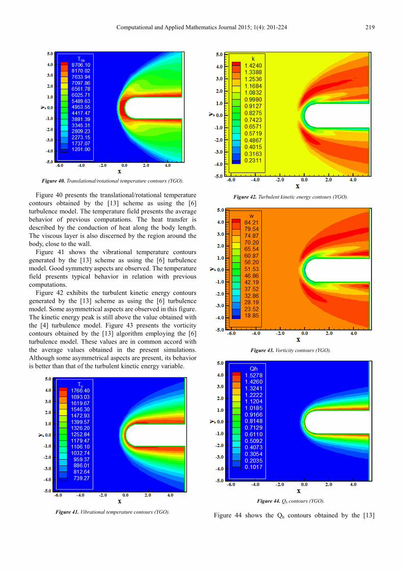
Figure 40. Translational/rotational temperature contours (YGO).
Figure 40 presents the translational/rotational temperature
contours obtained by the [13] scheme as using the [6]
turbulence model. The temperature field presents the average
behavior of previous computations. The heat transfer is
described by the conduction of heat along the body length.
The viscous layer is also discerned by the region around the
body, close to the wall.
Figure 41 shows the vibrational temperature contours
generated by the [13] scheme as using the [6] turbulence
model. Good symmetry aspects are observed. The temperature
field presents typical behavior in relation with previous
computations.
Figure 42 exhibits the turbulent kinetic energy contours
generated by the [13] scheme as using the [6] turbulence
model. Some asymmetrical aspects are observed in this figure.
The kinetic energy peak is still above the value obtained with
the [4] turbulence model. Figure 43 presents the vorticity
contours obtained by the [13] algorithm employing the [6]
turbulence model. These values are in common accord with
the average values obtained in the present simulations.
Although some asymmetrical aspects are present, its behavior
is better than that of the turbulent kinetic energy variable.
Figure 41. Vibrational temperature contours (YGO).
Figure 42. Turbulent kinetic energy contours (YGO).
Figure 43. Vorticity contours (YGO).
Figure 44. Qh contours (YGO).
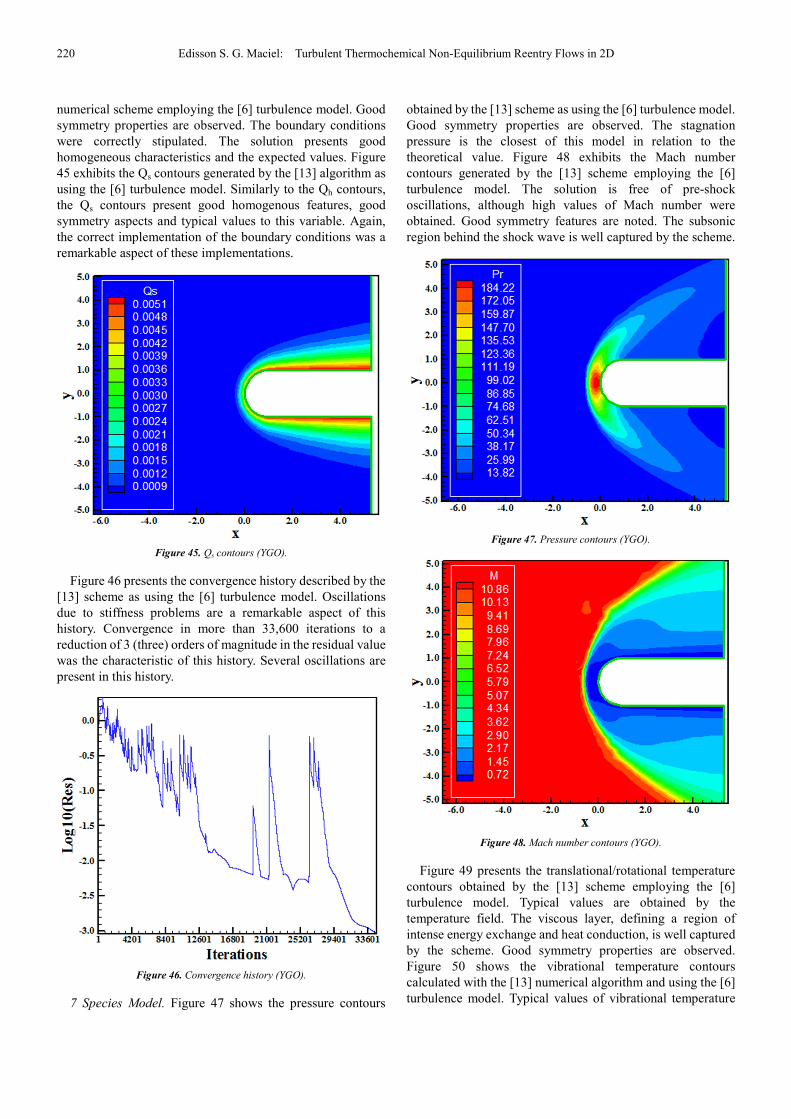
Figure 44 shows the Qh contours obtained by the [13]
220 Edisson S. G. Maciel: Turbulent Thermochemical Non-Equilibrium Reentry Flows in 2D
numerical scheme employing the [6] turbulence model. Good
symmetry properties are observed. The boundary conditions
were correctly stipulated. The solution presents good
homogeneous characteristics and the expected values. Figure
45 exhibits the Qs contours generated by the [13] algorithm as
using the [6] turbulence model. Similarly to the Qh contours,
the Qs contours present good homogenous features, good
symmetry aspects and typical values to this variable. Again,
the correct implementation of the boundary conditions was a
remarkable aspect of these implementations.
Figure 45. Qs contours (YGO).
Figure 46 presents the convergence history described by the
[13] scheme as using the [6] turbulence model. Oscillations
due to stiffness problems are a remarkable aspect of this
history. Convergence in more than 33,600 iterations to a
reduction of 3 (three) orders of magnitude in the residual value
was the characteristic of this history. Several oscillations are
present in this history.
Figure 46. Convergence history (YGO).
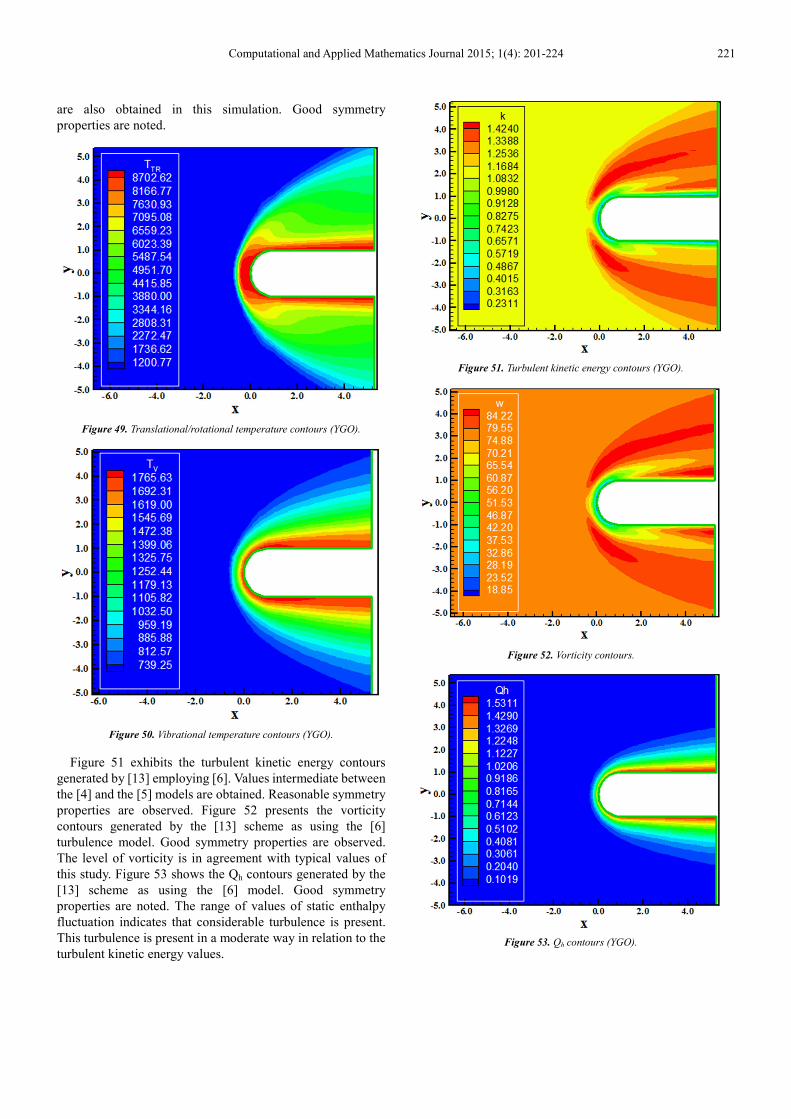
7 Species Model. Figure 47 shows the pressure contours
obtained by the [13] scheme as using the [6] turbulence model.
Good symmetry properties are observed. The stagnation
pressure is the closest of this model in relation to the
theoretical value. Figure 48 exhibits the Mach number
contours generated by the [13] scheme employing the [6]
turbulence model. The solution is free of pre-shock
oscillations, although high values of Mach number were
obtained. Good symmetry features are noted. The subsonic
region behind the shock wave is well captured by the scheme.
Figure 47. Pressure contours (YGO).
Figure 48. Mach number contours (YGO).
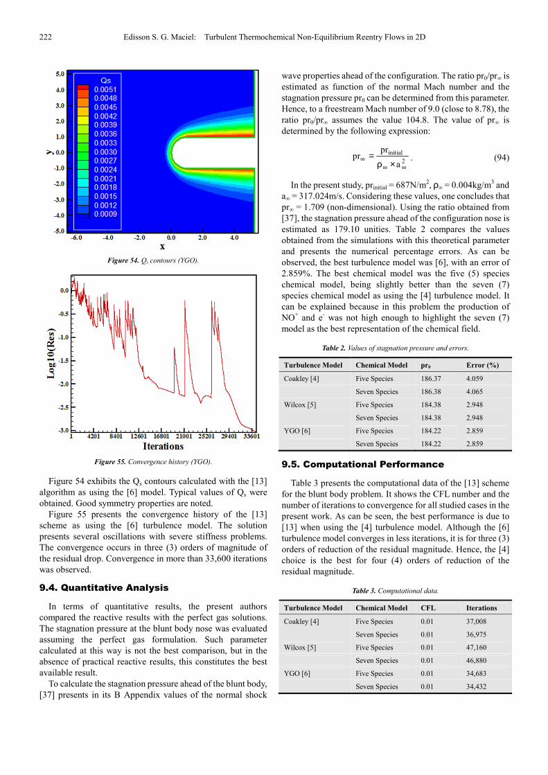
Figure 49 presents the translational/rotational temperature
contours obtained by the [13] scheme employing the [6]
turbulence model. Typical values are obtained by the
temperature field. The viscous layer, defining a region of
intense energy exchange and heat conduction, is well captured
by the scheme. Good symmetry properties are observed.
Figure 50 shows the vibrational temperature contours
calculated with the [13] numerical algorithm and using the [6]
turbulence model. Typical values of vibrational temperature
Computational and Applied Mathematics Journal 2015; 1(4): 201-224 221
are also obtained in this simulation. Good symmetry
properties are noted.
Figure 49. Translational/rotational temperature contours (YGO).
Figure 50. Vibrational temperature contours (YGO).
Figure 51 exhibits the turbulent kinetic energy contours
generated by [13] employing [6]. Values intermediate between
the [4] and the [5] models are obtained. Reasonable symmetry
properties are observed. Figure 52 presents the vorticity
contours generated by the [13] scheme as using the [6]
turbulence model. Good symmetry properties are observed.
The level of vorticity is in agreement with typical values of
this study. Figure 53 shows the Qh contours generated by the
[13] scheme as using the [6] model. Good symmetry
properties are noted. The range of values of static enthalpy
fluctuation indicates that considerable turbulence is present.
This turbulence is present in a moderate way in relation to the
turbulent kinetic energy values.
Figure 51. Turbulent kinetic energy contours (YGO).
Figure 52. Vorticity contours.
Figure 53. Qh contours (YGO).
222 Edisson S. G. Maciel: Turbulent Thermochemical Non-Equilibrium Reentry Flows in 2D
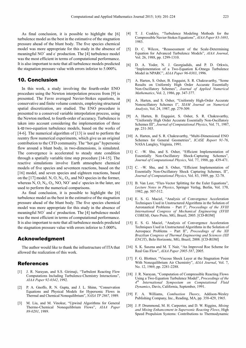
Figure 54. Qs contours (YGO).
Figure 55. Convergence history (YGO).
Figure 54 exhibits the Qs contours calculated with the [13]
algorithm as using the [6] model. Typical values of Qs were
obtained. Good symmetry properties are noted.
Figure 55 presents the convergence history of the [13]
scheme as using the [6] turbulence model. The solution
presents several oscillations with severe stiffness problems.
The convergence occurs in three (3) orders of magnitude of
the residual drop. Convergence in more than 33,600 iterations
was observed.
9.4. Quantitative Analysis
In terms of quantitative results, the present authors
compared the reactive results with the perfect gas solutions.
The stagnation pressure at the blunt body nose was evaluated
assuming the perfect gas formulation. Such parameter
calculated at this way is not the best comparison, but in the
absence of practical reactive results, this constitutes the best
available result.
To calculate the stagnation pressure ahead of the blunt body,
[37] presents in its B Appendix values of the normal shock
wave properties ahead of the configuration. The ratio pr0/pr∞ is
estimated as function of the normal Mach number and the
stagnation pressure pr0 can be determined from this parameter.
Hence, to a freestream Mach number of 9.0 (close to 8.78), the
ratio pr0/pr∞ assumes the value 104.8. The value of pr∞ is
determined by the following expression:
2
initial
a
prpr
∞∞∞
×ρ= . (94)
In the present study, prinitial = 687N/m2, ρ∞ = 0.004kg/m
3 and
a∞ = 317.024m/s. Considering these values, one concludes that
pr∞ = 1.709 (non-dimensional). Using the ratio obtained from
[37], the stagnation pressure ahead of the configuration nose is
estimated as 179.10 unities. Table 2 compares the values
obtained from the simulations with this theoretical parameter
and presents the numerical percentage errors. As can be
observed, the best turbulence model was [6], with an error of
2.859%. The best chemical model was the five (5) species
chemical model, being slightly better than the seven (7)
species chemical model as using the [4] turbulence model. It
can be explained because in this problem the production of
NO+ and e
- was not high enough to highlight the seven (7)
model as the best representation of the chemical field.
Table 2. Values of stagnation pressure and errors.
Turbulence Model Chemical Model pr0 Error (%)
Coakley [4] Five Species 186.37 4.059
Seven Species 186.38 4.065
Wilcox [5] Five Species 184.38 2.948
Seven Species 184.38 2.948
YGO [6] Five Species 184.22 2.859
Seven Species 184.22 2.859
9.5. Computational Performance
Table 3 presents the computational data of the [13] scheme
for the blunt body problem. It shows the CFL number and the
number of iterations to convergence for all studied cases in the
present work. As can be seen, the best performance is due to
[13] when using the [4] turbulence model. Although the [6]
turbulence model converges in less iterations, it is for three (3)
orders of reduction of the residual magnitude. Hence, the [4]
choice is the best for four (4) orders of reduction of the
residual magnitude.
Table 3. Computational data.
Turbulence Model Chemical Model CFL Iterations
Coakley [4] Five Species 0.01 37,008
Seven Species 0.01 36,975
Wilcox [5] Five Species 0.01 47,160
Seven Species 0.01 46,880
YGO [6] Five Species 0.01 34,683
Seven Species 0.01 34,432
Computational and Applied Mathematics Journal 2015; 1(4): 201-224 223
As final conclusion, it is possible to highlight the [6]
turbulence model as the best in the estimative of the stagnation
pressure ahead of the blunt body. The five species chemical
model was more appropriate for this study in the absence of
meaningful NO+ and e
- production. The [4] turbulence model
was the most efficient in terms of computational performance.
It is also important to note that all turbulence models predicted
the stagnation pressure value with errors inferior to 5.000%.
10. Conclusion
In this work, a study involving the fourth-order ENO
procedure using the Newton interpolation process from [9] is
presented. The Favre averaged Navier-Stokes equations, in
conservative and finite volume contexts, employing structured
spatial discretization, are studied. The ENO procedure is
presented to a conserved variable interpolation process, using
the Newton method, to fourth-order of accuracy. Turbulence is
taken into account considering the implementation of three
k-ω two-equation turbulence models, based on the works of
[4-6]. The numerical algorithm of [13] is used to perform the
reentry flow numerical experiments, which give us an original
contribution to the CFD community. The “hot gas” hypersonic
flow around a blunt body, in two-dimensions, is simulated.
The convergence is accelerated to steady state condition
through a spatially variable time step procedure [14-15]. The
reactive simulations involve Earth atmosphere chemical
models of five species and seventeen reactions, based on the
[16] model, and seven species and eighteen reactions, based
on the [17] model. N, O, N2, O2, and NO species in the former,
whereas N, O, N2, O2, NO, NO+ and e
- species in the later, are
used to perform the numerical comparisons.
As final conclusion, it is possible to highlight the [6]
turbulence model as the best in the estimative of the stagnation
pressure ahead of the blunt body. The five species chemical
model was more appropriate for this study in the absence of
meaningful NO+ and e
- production. The [4] turbulence model
was the most efficient in terms of computational performance.
It is also important to note that all turbulence models predicted
the stagnation pressure value with errors inferior to 5.000%.
Acknowledgment
The author would like to thank the infrastructure of ITA that
allowed the realization of this work.
References
[1] J. R. Narayan, and S.S. Girimaji, “Turbulent Reacting Flow Computations Including Turbulence-Chemistry Interactions”, AIAA Paper 92-0342, 1992.
[2] P. A. Gnoffo, R. N. Gupta, and J. L. Shinn, “Conservation Equations and Physical Models for Hypersonic Flows in Thermal and Chemical Nonequilibrium”, NASA TP 2867, 1989.
[3] M. Liu, and M. Vinokur, “Upwind Algorithms for General Thermo-Chemical Nonequilibrium Flows”, AIAA Paper 89-0201, 1989.
[4] T. J. Coakley, “Turbulence Modeling Methods for the Compressible Navier-Stokes Equations”, AIAA Paper 83-1693, 1983.
[5] D. C. Wilcox, “Reassessment of the Scale-Determining Equation for Advanced Turbulence Models”, AIAA Journal, Vol. 26, 1988, pp. 1299-1310.
[6] D. A. Yoder, N. J. Georgiadids, and P. D. Orkwis, “Implementation of a Two-Equation K-Omega Turbulence Model in NPARC”, AIAA Paper 96-0383, 1996.
[7] A. Harten, S. Osher, B. Engquist, S. R. Chakravarthy, “Some Results on Uniformly High Order Accurate Essentially Non-Oscillatory Schemes”, Journal of Applied Numerical Mathematics, Vol. 2, 1986, pp. 347-377.
[8] A. Harten, and S. Osher, “Uniformly High-Order Accurate Nonoscillatory Schemes I”, SIAM Journal on Numerical Analysis, Vol. 24, 1987, pp. 279-309.
[9] A. Harten, B. Engquist, S. Osher, S. R. Chakravarthy, “Uniformly High Order Accurate Essentially Non-Oscillatory Schemes III”, Journal of Computational Physics, Vol. 71, 1987, pp. 231-303.
[10] A. Harten, and S. R. Chakravarthy, “Multi-Dimensional ENO Schemes for General Geometries”, ICASE Report 91-76, NASA Langley, Virginia, 1991.
[11] C. –W. Shu, and S. Osher, “Efficient Implementation of Essentially Non-Oscillatory Shock-Capturing Schemes”, Journal of Computational Physics, Vol. 77, 1988, pp. 439-471.
[12] C. –W. Shu, and S. Osher, “Efficient Implementation of Essentially Non-Oscillatory Shock Capturing Schemes, II”, Journal of Computational Physics, Vol. 83, 1989, pp. 32-78.
[13] B. Van Leer, “Flux-Vector Splitting for the Euler Equations”, Lecture Notes in Physics, Springer Verlag, Berlin, Vol. 170, 1982, pp. 507-512.
[14] E. S. G. Maciel, “Analysis of Convergence Acceleration Techniques Used in Unstructured Algorithms in the Solution of Aeronautical Problems – Part I”, Proceedings of the XVIII International Congress of Mechanical Engineering (XVIII COBEM), Ouro Preto, MG, Brazil, 2005. [CD-ROM]
[15] E. S. G. Maciel, “Analysis of Convergence Acceleration Techniques Used in Unstructured Algorithms in the Solution of Aerospace Problems – Part II”, Proceedings of the XII Brazilian Congress of Thermal Engineering and Sciences (XII ENCIT), Belo Horizonte, MG, Brazil, 2008. [CD-ROM]
[16] S. K. Saxena and M. T. Nair, “An Improved Roe Scheme for Real Gas Flow”, AIAA Paper 2005-587, 2005.
[17] F. G. Blottner, “Viscous Shock Layer at the Stagnation Point With Nonequilibrium Air Chemistry”, AIAA Journal, Vol. 7, No. 12, 1969, pp. 2281-2288.
[18] J. R. Narayan, “Computation of Compressible Reacting Flows Using a Two-Equation Turbulence Model”, Proceedings of the 4th International Symposium on Computational Fluid Dynamics, Davis, California, September, 1991.
[19] F. A. Williams, Combustion Theory, Addison-Wesley Publishing Company, Inc., Reading, MA, pp. 358-429, 1965.
[20] J. P. Drummond, M. H. Carpenter, and D. W. Riggins, Mixing and Mixing Enhancement in Supersonic Reacting Flows, High Speed Propulsion Systems: Contributions to Thermodynamic
224 Edisson S. G. Maciel: Turbulent Thermochemical Non-Equilibrium Reentry Flows in 2D
Analysis, ed. E. T. Curran and S. N. B. Murthy, American Institute of Astronautics and Aeronautics (AIAA), Washington, D. C., 1990.
[21] E. S. G. Maciel, and A. P. Pimenta, “Thermochemical Non-Equilibrium Reentry Flows in Two-Dimensions – Part I”, WSEAS Transactions on Mathematics, Vol. 11, Issue 6, 2012, pp. 520-545.
[22] E. S. G. Maciel, and A. P. Pimenta, “Thermochemical Non-Equilibrium Reentry Flows in Two-Dimensions – Part II”, WSEAS Transactions on Mathematics, Vol. 11, Issue 11, 2012, pp. 977-1005.
[23] E. S. G. Maciel, and A. P. Pimenta, “Thermochemical Non-Equilibrium Reentry Flows in Two-Dimensions: Seven Species Model – Part I”, WSEAS Transactions on Applied and Theoretical Mechanics, Vol. 7, Issue 4, 2012, pp. 311-337.
[24] E. S. G. Maciel, and A. P. Pimenta, “Thermochemical Non-Equilibrium Reentry Flows in Two-Dimensions: Seven Species Model – Part II”, WSEAS Transactions on Applied and Theoretical Mechanics, Vol. 8, Issue 1, 2013, pp. 55-83.
[25] A. Favre, Statistical Equations of Turbulent Gases, Institut de Mechanique Statistique de la Turbulence, Marseille.
[26] F. H. Harlow, and P. I. Nakayama, “Turbulence Transport Equations”, The Physics of Fluids, Vol. 10, No. 11, 1967, pp. 2323-2332.
[27] K. Hanjalic, and B. E., Launder, “A Reynolds Stress Model of Turbulence and its Application to Thin Shear Flows”, J. Fluid Mech., Vol. 52, Part 4, 1972, pp. 609-638.
[28] S. S. Girimaji, “A Simple Recipe for Modeling Reaction-Rates in Flows with Turbulent Combustion”, AIAA Paper 91-1792, 1991.
[29] R. K. Prabhu, “An Implementation of a Chemical and Thermal Nonequilibrium Flow Solver on Unstructured Meshes and Application to Blunt Bodies”, NASA CR-194967, 1994.
[30] D. Ait-Ali-Yahia, and W. G. Habashi, “Finite Element Adaptive Method for Hypersonic Thermochemical Nonequilibrium Flows”, AIAA Journal Vol. 35, No. 8, 1997, 1294-1302.
[31] R. Radespiel, and N. Kroll, “Accurate Flux Vector Splitting for Shocks and Shear Layers”, Journal of Computational Physics, Vol. 121, 1995, pp. 66-78.
[32] L. N. Long, M. M. S. Khan, and H. T. Sharp, “Massively Parallel Three-Dimensional Euler / Navier-Stokes Method”, AIAA Journal, Vol. 29, No. 5, 1991, pp. 657-666.
[33] J. J. Van Der Vegt, “ENO-Osher Schemes for Euler Equations”, AIAA Paper 93-0335, 1993.
[34] E. S. G. Maciel, “Assessment of Several Turbulence Models as Applied to Supersonic Flows in 2D – Part II”, Submitted to Engineering and Technology (under review), 2015.
[35] R. W. Fox, and A. T. McDonald, Introdução à Mecânica dos Fluidos, Guanabara Editor, 1988.
[36] E. S. G. Maciel, “High Order Comparison Between Flux Vector Splitting Schemes on the Reentry Flow Context”, Submitted to the Computational and Applied Mathematics Journal (under review), 2015.
[37] J. D. Anderson Jr., Fundamentals of Aerodynamics, McGraw-Hill, Inc., 5th Edition, 1008p., 2010.