
Extreme Ultraviolet Variability Experiment (EVE) Multiple...
34
Solar Phys DOI 10.1007/s11207-010-9520-9 THE SOLAR DYNAMICS OBSERVATORY Extreme Ultraviolet Variability Experiment (EVE) Multiple EUV Grating Spectrographs (MEGS): Radiometric Calibrations and Results R.A. Hock · P.C. Chamberlin · T.N. Woods · D. Crotser · F.G. Eparvier · D.L. Woodraska · E.C. Woods Received: 6 October 2009 / Accepted: 20 January 2010 © The Author(s) 2010. This article is published with open access at Springerlink.com Abstract The NASA Solar Dynamics Observatory (SDO), scheduled for launch in early 2010, incorporates a suite of instruments including the Extreme Ultraviolet Variability Ex- periment (EVE). EVE has multiple instruments including the Multiple Extreme ultraviolet Grating Spectrographs (MEGS) A, B, and P instruments, the Solar Aspect Monitor (SAM), and the Extreme ultraviolet SpectroPhotometer (ESP). The radiometric calibration of EVE, necessary to convert the instrument counts to physical units, was performed at the National Institute of Standards and Technology (NIST) Synchrotron Ultraviolet Radiation Facility (SURF III) located in Gaithersburg, Maryland. This paper presents the results and derived accuracy of this radiometric calibration for the MEGS A, B, P, and SAM instruments, while the calibration of the ESP instrument is addressed by Didkovsky et al. (Solar Phys., 2010, doi:10.1007/s11207-009-9485-8). In addition, solar measurements that were taken on 14 April 2008, during the NASA 36.240 sounding-rocket flight, are shown for the prototype EVE instruments. Keywords SDO · EVE · Solar EUV irradiance · Calibration · Synchrotron 1. Introduction The Solar Dynamics Observatory (SDO) is the first mission in NASA’s Living With a Star (LWS) program. The goal of SDO is to quantify and understand the causes of solar vari- ability and its effects on Earth. The Extreme Ultraviolet Variability Experiment (EVE), one The Solar Dynamics Observatory Guest Editors: W. Dean Pesnell, Phillip C. Chamberlin, and Barbara J. Thompson. R.A. Hock ( ) · T.N. Woods · D. Crotser · F.G. Eparvier · D.L. Woodraska Laboratory for Atmospheric and Space Physics, 1234 Innovation Drive, Boulder, CO 80303, USA e-mail: [email protected] P.C. Chamberlin Solar Physics Laboratory, Code 671, NASA Goddard Space Flight Center, Greenbelt, MD 20771, USA E.C. Woods Rhodes College, 2000 North Parkway, Memphis, TN 38112, USA
Transcript of Extreme Ultraviolet Variability Experiment (EVE) Multiple...
Solar PhysDOI 10.1007/s11207-010-9520-9
T H E S O L A R DY NA M I C S O B S E RVAT O RY
Extreme Ultraviolet Variability Experiment (EVE)Multiple EUV Grating Spectrographs (MEGS):Radiometric Calibrations and Results
R.A. Hock · P.C. Chamberlin · T.N. Woods · D. Crotser ·F.G. Eparvier · D.L. Woodraska · E.C. Woods
Received: 6 October 2009 / Accepted: 20 January 2010© The Author(s) 2010. This article is published with open access at Springerlink.com
Abstract The NASA Solar Dynamics Observatory (SDO), scheduled for launch in early2010, incorporates a suite of instruments including the Extreme Ultraviolet Variability Ex-periment (EVE). EVE has multiple instruments including the Multiple Extreme ultravioletGrating Spectrographs (MEGS) A, B, and P instruments, the Solar Aspect Monitor (SAM),and the Extreme ultraviolet SpectroPhotometer (ESP). The radiometric calibration of EVE,necessary to convert the instrument counts to physical units, was performed at the NationalInstitute of Standards and Technology (NIST) Synchrotron Ultraviolet Radiation Facility(SURF III) located in Gaithersburg, Maryland. This paper presents the results and derivedaccuracy of this radiometric calibration for the MEGS A, B, P, and SAM instruments, whilethe calibration of the ESP instrument is addressed by Didkovsky et al. (Solar Phys., 2010,doi:10.1007/s11207-009-9485-8). In addition, solar measurements that were taken on 14April 2008, during the NASA 36.240 sounding-rocket flight, are shown for the prototypeEVE instruments.
Keywords SDO · EVE · Solar EUV irradiance · Calibration · Synchrotron
1. Introduction
The Solar Dynamics Observatory (SDO) is the first mission in NASA’s Living With a Star(LWS) program. The goal of SDO is to quantify and understand the causes of solar vari-ability and its effects on Earth. The Extreme Ultraviolet Variability Experiment (EVE), one
The Solar Dynamics ObservatoryGuest Editors: W. Dean Pesnell, Phillip C. Chamberlin, and Barbara J. Thompson.
R.A. Hock (�) · T.N. Woods · D. Crotser · F.G. Eparvier · D.L. WoodraskaLaboratory for Atmospheric and Space Physics, 1234 Innovation Drive, Boulder, CO 80303, USAe-mail: [email protected]
P.C. ChamberlinSolar Physics Laboratory, Code 671, NASA Goddard Space Flight Center, Greenbelt, MD 20771, USA
E.C. WoodsRhodes College, 2000 North Parkway, Memphis, TN 38112, USA
R.A. Hock et al.
of the three experiments on SDO, will measure the variability of the Sun’s irradiance in theX-ray ultraviolet (XUV) and extreme ultraviolet (EUV) wavelengths from 0.1 to 106 nmplus the hydrogen Lyman-α emission line at 121.6 nm. The EVE irradiance measurementswill be made with better than 25% accuracy over the mission lifetime.
Details about EVE can be found in Woods et al. (2010), which includes the science (mea-surements and modeling) goals, as well as the details of the EVE instrument design anddata products. The calibration and algorithms of the Multiple EUV Grating Spectrographs(MEGS) A, B, P, and Solar Aspect Monitor (SAM) instruments are the focus of this paper.The results shown are from the final EVE calibration performed at the National Institute ofStandards and Technology (NIST) Synchrotron Ultraviolet Radiation Facility III (SURF III)in Gaithersburg, Maryland, during August 2007. Also included are results from a January2009 calibration of the prototype EVE instrument that will be flown as an underflight cali-bration three months after SDO launches. A brief overview of the EVE instruments is givenin Section 2, followed by a discussion of EVE’s calibration heritage in Section 3. The SURFIII radiometric calibration facilities are detailed in Section 4, then the calibration algorithmsand results of the MEGS A and B instruments are presented in Section 5, followed by adiscussion of the MEGS P and SAM calibrations in Sections 6 and 7, respectively. The solarEUV spectral irradiance from a sounding-rocket flight on 14 April 2008 using the prototypeEVE instrument is then presented in Section 8, followed by concluding remarks in Section 9.
2. EVE Instruments
The EVE instrument suite will measure the solar spectral irradiance from 0.1 to 6 nm with1-nm spectral resolution, 6 to 106 nm with 0.1-nm resolution, and the hydrogen Lyman-αline at 121.6 nm with 1-nm resolution. Solar observations will be taken continuously with aten-second cadence except during satellite eclipse periods and planned calibration activities,which are expected to total less than 1% of the mission lifetime. To cover the entire spectralrange and meet accuracy requirements, EVE is composed of multiple instruments. The EVEinstrument design is described in detail by Woods et al. (2010), so only a brief overview ofthe instruments is given here.
The primary, high-spectral-resolution irradiance measurements are made by the MEGS Aand B instruments. MEGS A is an off-Rowland-circle grazing-incidence spectrograph cov-ering the 6 to 37 nm range. The entrance aperture of MEGS A includes two slits: denotedA1 and A2. Light illuminating these slits shares the same grating and CCD detector, buthas light paths that are offset in the cross-dispersion direction of the grating and thereforedo not overlap on the CCD. In addition, MEGS A1 and A2 have separate primary filterswith different spectral bandpasses to isolate different portions of the MEGS A wavelengthrange and reduce the effects from higher orders. MEGS A1 is optimized for the 6 to 18 nmrange, while MEGS A2 covers 16 to 37 nm. MEGS B is a two-grating, cross-dispersingspectrograph covering the 36 to 106 nm range. The two orthogonal gratings are designedto eliminate the out-of-band light without the use of a bandpass filter and to disperse thehigher-order spectra off the primary first-order spectrum.
Both MEGS A and B use the same type of 2048 × 1024 CCD. Westhoff et al. (2007)provide more information about the CCDs used with MEGS. Ray-tracing results for theMEGS spectrometers are found in Crotser et al. (2004, 2007). The MEGS CCDs are two-dimensional arrays. One direction, the dispersion direction, covers the wavelength range ofthe instrument over 2048 pixels. The other direction, the cross-dispersion direction, imagesthe slit at each wavelength over 1024 pixels. As a result, the solar irradiance for any given
Extreme Ultraviolet Variability Experiment (EVE) Multiple EUV
wavelength is spread over many pixels in the cross-dispersion direction of the CCD. Wecreate our final science products by adding together all pixels with a certain wavelength.
MEGS P measures the Lyman-α emission with 0.25-second cadence using a Si photo-diode. Lyman-α is isolated by placing the diode in the MEGS B optical path at the pointwhere 121.6 nm photons are dispersed after MEGS B’s first grating. A limiting bandpassLyman-α filter is also used to eliminate potentially significant out-of-band light.
Included as part of the MEGS A package is SAM: a pinhole camera that observes theshort XUV wavelengths (0.1 – 7 nm). SAM is designed to record single photon events thatcan be used to reconstruct a spectrum with 1-nm spectral resolution. In addition, SAM hasthe ability to generate images with a coarse spatial resolution of approximately 15 arcsec-onds per pixel.
The EUV SpectroPhotometer (ESP) instrument uses a transmission grating to disperseEUV light onto a set of broadband EUV photometers. This instrument will not only gethigher temporal resolution measurements (0.25 seconds), but will also, along with under-flight calibration rockets, help quantify and track the long-term degradation of the MEGSinstruments. As ESP’s diodes are expected to degrade slowly over time, they can help tore-calibrate MEGS results if MEGS undergoes a sudden change in responsivity from a CCDbakeout or science-filter failure. While the absolute calibration of EVE will be tied to theplanned annual rocket underflights, ESP and MEGS P can help track degradation trends be-tween rocket flights. The details of the ESP instrument are presented by Didkovsky et al.(2010).
All instruments on EVE have a rotatable filter wheel in front of their entrance apertures.These filter wheels house redundant science filters, which may be necessary in the event thata primary science filter develops pinholes. There are also blank filter positions that allow fordark measurements on orbit. One filter position in each of the MEGS A and B filter holderscontains a “second-order filter” that blocks the short-wavelength portion of the primary filterand quantifies the effects of higher grating orders. Other positions have filters that transmitvisible light to check for out-of-band scattered light. Triplett et al. (2007) give calibrationresults for the EVE filters.
3. EVE MEGS Calibration Heritage
The MEGS instruments on EVE are a follow-on to the Solar EUV Experiment (SEE) thathas been making measurements since February 2002 of the solar spectral irradiance from0.1 to 195 nm onboard the Thermosphere, Ionosphere, Mesosphere Energetics and Dynam-ics (TIMED) satellite (Woods et al., 2005). Although EVE has a limited spectral range com-pared to SEE, EVE will improve upon the temporal and spectral resolution, accuracy, andduty cycle. Currently, SEE is planned to overlap with EVE in time to compare the absolutevalues of the two experiments and create a continuous record of the solar EUV irradiance.
SEE has provided experience not only in designing and building the EUV spectrographsand photometers, but also in determining the radiometric calibration. For example, the EUVGrating Spectrograph (EGS), an instrument on SEE and a copy for underflight rocket pay-loads, has been calibrated at SURF more than eight times. This includes two calibrationsof the flight EGS before launch as well as several calibrations of the rocket underflightcopy. Another instrument, the X-ray Photometer System (XPS) has been flown as differ-ent versions on the Student Nitric Oxide Experiment (SNOE; Bailey et al., 2006), TIMED(Woods et al., 2005), and the Solar Radiation and Climate Experiment (SORCE; Woodsand Rottman, 2005) as well as a prototype version that has flown on various sounding rocket
R.A. Hock et al.
flights. As a result, it has been calibrated at SURF numerous times. The TIMED/SEE cali-brations and algorithms are described by Woods et al. (2005), while the SORCE/XPS cali-brations and results are given by Woods, Rottman, and Vest (2005).
4. SURF Calibration Setup
The primary EVE calibrations are performed in the vacuum chamber at the end of beamline 2 (BL-2) at the SURF III calibration facility in Gaithersburg, Maryland. SURF providesa primary radiometric source that is accurate to 1%, one of the most accurate UV sourcesavailable (Arp et al., 2000). There are certain advantages of using this primary source overusing secondary, transfer standards that were first calibrated at NIST. Calibrating at SURFnot only eliminates the uncertainties associated with using a transfer standard but also pro-vides an adjustable source in both intensity and wavelength that provides flexibility to opti-mize many of the calibrations discussed throughout this paper. The key calibration parame-ters for the SURF beam are the beam energy, which determines the peak wavelength, andthe beam current, which determines the intensity.
At SURF, the EVE instruments are coherently illuminated by the synchrotron radiationfrom the electrons that travel around the SURF ring with a frequency of 57 MHz. Thediffraction effects from BL-2 baffles are minimized to less than 1% for the EVE calibrations.First, by having the EVE entrance slit smaller than the SURF illuminated beam size and alsohaving the slit located in the center of the beam, the beam line baffle diffraction patternsdo not enter the MEGS slits. Furthermore, the EVE grating is much larger than the slitdiffraction pattern incident on the grating; thereby, the majority of the radiation reaches thedetector. Consequently, no corrections for diffraction are made in the MEGS algorithms.
EVE is mounted in a vacuum chamber that allows the entire system, from electron ringto instrument CCDs, to be in a vacuum environment, thus eliminating any influence or ab-sorption of the EUV photons by air or glass windows. Inside the vacuum chamber, EVE ismounted to a gimbal system that provides pitch and yaw movements. This allows the field-of-view (FOV), or the angle of the SURF beam relative to the normal of the entrance slit,to vary. As the SURF beam is much smaller that the angular size of the Sun, it is importantto vary the FOV to characterize the resulting changes in the optical responses. The vacuumchamber also allows for x- and y-translations in order to center the SURF beam in the middleof the aperture for each EVE instrument.
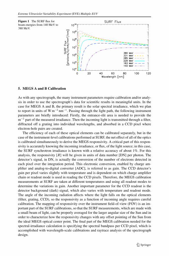
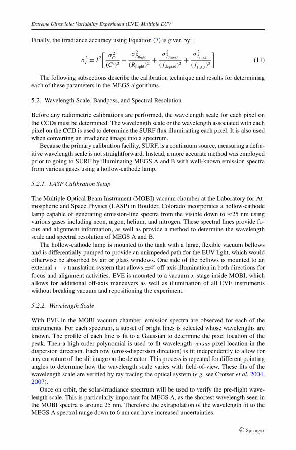
Both the beam energy and current determine the photon flux from the SURF beam. Thebeam energy determines the spectral shape, while the current determines the intensity. Fig-ure 1 shows the photon flux per milliamp of SURF current for each beam energy used in theEVE calibrations. Lower energies shift the peak intensity to longer wavelengths and havefewer photons per unit current. As a result, using lower energies requires higher currentsto provide a similar photon flux into the instrument. Most calibrations were done using the380 MeV beam energy. The current was adjusted to get high counts but not so high as tosaturate any of the CCD’s pixels. Correcting for the effects of higher orders requires usingmultiple energies; the details of this process are discussed in Section 5.4.4.
In general, to improve the counting statistics and reduce uncertainties, at least 20 ten-second images are co-added for each calibration test. Furthermore, each instrument is cali-brated separately to allow us to optimize the beam current and energy. Once all of the cali-bration data have been taken, these data need to be processed to obtain the final responsivityfor each of the EVE instruments.
Extreme Ultraviolet Variability Experiment (EVE) Multiple EUV
Figure 1 The SURF flux forbeam energies from 140 MeV to380 MeV.
5. MEGS A and B Calibration
As with any spectrograph, the many instrument parameters require calibration and/or analy-sis in order to use the spectrograph’s data for scientific results in meaningful units. In thecase for MEGS A and B, the primary result is the solar spectral irradiance, which we planto report in units of W m−2 nm−1. Passing through the light path, the following instrumentparameters are briefly introduced: Firstly, the entrance-slit area is needed to provide them−2 part of the measured irradiance. Then the incoming light is transmitted through a filter,diffracted off a grating into individual wavelengths, and absorbed in a CCD pixel whereelectron-hole pairs are created.
The efficiency of each of these optical elements can be calibrated separately, but in thecase of the instrument-level calibrations performed at SURF, the net effect of all of the opticsis calibrated simultaneously to derive the MEGS responsivity. A critical part of this respon-sivity is accurately knowing the incoming irradiance, or flux, of the light source; in this case,the SURF synchrotron irradiance is known with a relative accuracy of about 1%. For thisanalysis, the responsivity [R] will be given in units of data number [DN] per photon. Thedetector’s signal, in DN, is actually the conversion of the number of electrons detected ineach pixel over the integration period. This electronic conversion, enabled by charge am-plifier and analog-to-digital converter [ADC], is referred to as gain. The CCD detector’sgain per pixel varies slightly with temperature and is dependent on which charge amplifierchain or readout mode is used in reading the CCD pixels. Therefore, the MEGS calibrationmeasurements at SURF are taken at different temperatures and using all readout modes todetermine the variations in gain. Another important parameter for the CCD readout is thedetector background (dark) signal, which also varies with temperature and readout mode.The angle of the incoming radiation affects where the light falls on the optical elements(filter, grating, CCD), so the responsivity as a function of incoming angle requires carefulcalibration. The mapping of responsivity over the instrument field-of-view (FOV) is an im-portant part of the SURF calibrations, so that the SURF measurements, which are made witha small beam of light, can be properly averaged for the larger angular size of the Sun and inorder to characterize how the responsivity changes with any offset pointing of the Sun fromthe ideal MEGS optical center point. The final part of the MEGS calibration needed for thespectral-irradiance calculation is specifying the spectral bandpass per CCD pixel, which isaccomplished with wavelength-scale calibrations and raytrace analysis of the spectrographdesign.
R.A. Hock et al.
While MEGS A and B have different optical designs as discussed in Section 2 and inmore detail by Woods et al. (2010), the data from these instruments are calibrated andprocessed in the same way, as both instruments have the same type of CCDs. This sectionpresents the algorithms and calibration results for MEGS A1, A2, and B. The first subsec-tion, Section 5.1, discusses the algorithms necessary to convert CCD detector counts in DNto irradiance in W m−2 nm−1. Section 5.2 discusses the determination of the wavelengthscale and spectral resolution, while Sections 5.3 and 5.4 present the details of the algorithmsand calibration results. While the focus of this paper is on the calibration of the EVE instru-ments to be flown on SDO, final calibration results for the prototype EVE instrument flownon a NASA sounding rocket in 2008 are included for comparison. Some early calibrationresults for MEGS are presented by Chamberlin et al. (2007, 2009).
5.1. MEGS A and B Algorithms
There are two aspects of the MEGS algorithms: One is the responsivity algorithm usingthe SURF calibration measurements, and the other is the irradiance algorithm for the so-lar observations. These two algorithms are in concept identical, but inverted, equations. Forthe SURF calibrations, the responsivity is calculated as the measured signal divided by theknown synchrotron irradiance. For the solar observations, the solar spectral irradiance is cal-culated as the measured signal divided by the instrument responsivity derived from SURFcalibrations. In actuality, the algorithms are more detailed as the responsivity parameters aredependent on temperature and field-of-view angle, as well as other effects such as gratinghigher-order contributions to the measured signals. The following describes the algorithmsfor the MEGS signal, responsivity, and solar irradiance. The many parameters in these algo-rithms require characterization, from direct calibration and/or from analysis. The subsequentsections describe the calibration techniques and results for each of the primary instrumentparameters.
For MEGS A and B, the responsivity is calculated for each individual pixel on the2048 × 1024 CCD detectors, denoted by the indices i and j in the following equations.This pixel-based calibration allows us to bypass the flatfield correction sometimes used forarray detectors. Furthermore, the calibration is not based on calibrations of each individ-ual optical element of the instrument, but it is for the complete end-to-end optical system,including filter transmissions as well as grating and detector efficiencies.
The algorithms for the rocket instrument (prototype EVE) are essentially the same asthose for the flight EVE. As the rocket version of MEGS does not have a filter wheel, cali-brations were done for the primary (and only) filter, which is the same type as the primaryscience filters on the EVE flight instrument.
The first step for processing all MEGS A and B images, taken either at SURF or on orbitfor solar observations, is to correct the raw images to get the corrected count rate [C ′] inDN second−1:
C ′(i, j, t) =[
C(i, j, t, TCCD, tap)
�t− D(i, j, TCCD,C, tap)
]
× G(i, j, TCCD, tap)Mask(i, j,C, tap) (1)
The raw counts [C] in each pixel are corrected for the integration time [�t], dark offset [D],and the dependence of the CCDs on the temperature and readout mode [tap] of the electron-ics [G]. In addition, invalid pixels are identified and set to zero by applying a binary mask[Mask], allowing them to be ignored in later steps. While there are very few defective pixels
Extreme Ultraviolet Variability Experiment (EVE) Multiple EUV
on the CCDs, there are several pixels contaminated in each image by cosmic-ray particlehits during ground calibration and also by energetic particle hits during flight. The details ofhow each of these corrections are calculated will be discussed in Section 5.3.
Images taken at SURF are further processed to determine the SURF response [RSURF] inDN photon−1:
RSURF(i, j,Ebeam,filter, α,β) =1n
∑n
k=1C′
k(i,j,t,Ebeam,filter,α,β)
ISURF(t)
FSURF(i, j,Ebeam, α,β)Aslit�λ(i, j)(2)
Each corrected image [C ′] is normalized by the SURF beam current [ISURF] in mA. Then,all images taken with the same beam energy [Ebeam], filter, and field-of-view pointing [α,β]are co-added to reduce the uncertainty. Finally, this co-added image is divided by the SURFbeam flux [FSURF] in photons s−1 mA−1 mm−2 nm−1, area of the limiting aperture [Aslit]in mm2, and bandpass [�λ] in nm to derive the SURF response [RSURF].
The corrected counts used to determine the SURF response in Equation (2) can containboth first order and higher orders. As shown later, MEGS B SURF calibrations have es-sentially no higher-order contributions, so Equation (2) can be directly used for MEGS B.MEGS A responsivities do have contributions from higher orders so RSURF needs to be ad-justed to include only the first-order response. Equation (5) shows the relationship betweenRSURF and true first-order response [R1] as derived from:
RSURF(i, j,Ebeam,filter, α,β) =m∑
k=1
1
k
F kSURF(i, j,Ebeam, α,β)
F k=1SURF(i, j,Ebeam, α,β)
Rk(i, j,filter, α,β) (3)
where k denotes the order and
FkSURF(λ) = FSURF
(λ
k
)(4)
The contributions of the higher orders are found and separated by a proven method thatutilizes multiple beam energies at SURF (Saloman, 1975; Rottman, Woods, and Sparn,1993; Chamberlin, Woods, and Eparvier, 2002). This multiple-beam-energy method exploitsthe differences in the spectral distribution of SURF fluxes for different beam energies tovary RSURF. Using Equation (3), a system of linear equations can be written and then solvednumerically to determine each Rk . By using two different SURF beam energies, first andsecond order can be separated; using three energies, it is possible to calculate the contri-butions from first, second, and third orders. The results of this order-sorting correction areapplied as a scalar correction to RSURF:
fOS(i, j,Ebeam,filter, α,β) = R1(i, j,filter, α,β)
RSURF(i, j,Ebeam,filter, α,β)(5)
Determining RSURF and the higher-order correction will be discussed in Section 5.4.For processing solar data, the SURF response is used to calculate the flight responsivity
[Rflight] in DN s−1 (W m−2 nm−1)−1:
Rflight(i, j,filter)
= λ(i, j)
hc
[∑α,β
w(α,β)RSURF(i, j,Ebeam,filter, α,β)fOS(i, j,Ebeam,filter, α,β)
]
× Aslit�λ(i, j) (6)
R.A. Hock et al.
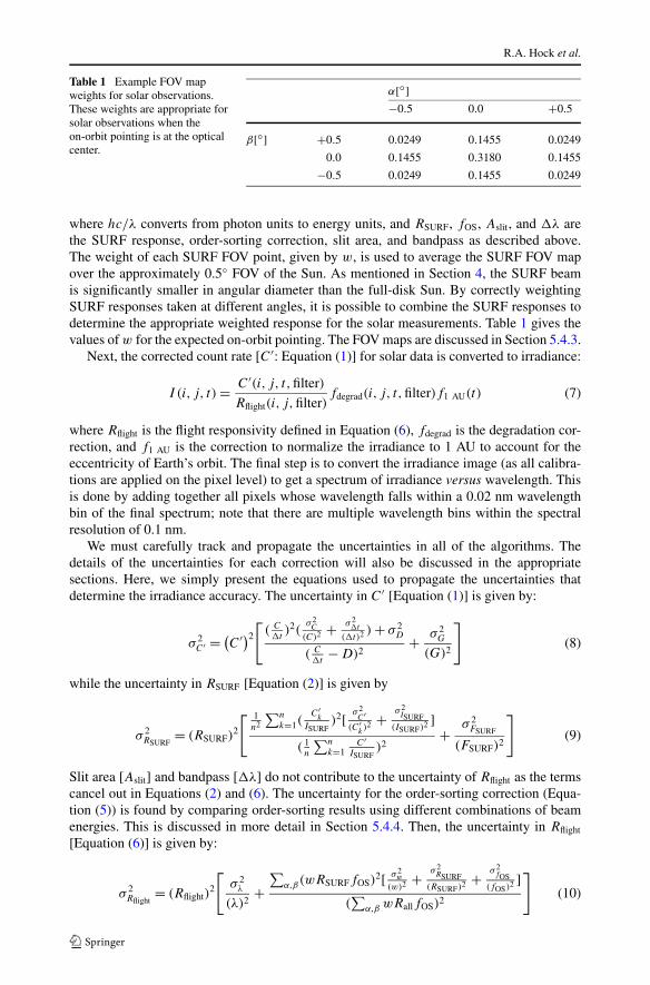
Table 1 Example FOV mapweights for solar observations.These weights are appropriate forsolar observations when theon-orbit pointing is at the opticalcenter.
α[◦]−0.5 0.0 +0.5
β[◦] +0.5 0.0249 0.1455 0.0249
0.0 0.1455 0.3180 0.1455
−0.5 0.0249 0.1455 0.0249
where hc/λ converts from photon units to energy units, and RSURF, fOS, Aslit, and �λ arethe SURF response, order-sorting correction, slit area, and bandpass as described above.The weight of each SURF FOV point, given by w, is used to average the SURF FOV mapover the approximately 0.5◦ FOV of the Sun. As mentioned in Section 4, the SURF beamis significantly smaller in angular diameter than the full-disk Sun. By correctly weightingSURF responses taken at different angles, it is possible to combine the SURF responses todetermine the appropriate weighted response for the solar measurements. Table 1 gives thevalues of w for the expected on-orbit pointing. The FOV maps are discussed in Section 5.4.3.
Next, the corrected count rate [C ′: Equation (1)] for solar data is converted to irradiance:
I (i, j, t) = C ′(i, j, t,filter)
Rflight(i, j,filter)fdegrad(i, j, t,filter)f1 AU(t) (7)
where Rflight is the flight responsivity defined in Equation (6), fdegrad is the degradation cor-rection, and f1 AU is the correction to normalize the irradiance to 1 AU to account for theeccentricity of Earth’s orbit. The final step is to convert the irradiance image (as all calibra-tions are applied on the pixel level) to get a spectrum of irradiance versus wavelength. Thisis done by adding together all pixels whose wavelength falls within a 0.02 nm wavelengthbin of the final spectrum; note that there are multiple wavelength bins within the spectralresolution of 0.1 nm.
We must carefully track and propagate the uncertainties in all of the algorithms. Thedetails of the uncertainties for each correction will also be discussed in the appropriatesections. Here, we simply present the equations used to propagate the uncertainties thatdetermine the irradiance accuracy. The uncertainty in C ′ [Equation (1)] is given by:
σ 2C′ = (
C ′)2
[( C
�t)2(
σ 2C
(C)2 + σ 2�t
(�t)2 ) + σ 2D
( C�t
− D)2+ σ 2
G
(G)2
](8)
while the uncertainty in RSURF [Equation (2)] is given by
σ 2RSURF
= (RSURF)2
[ 1n2
∑n
k=1(C′
k
ISURF)2[ σ 2
C′(C′
k)2 + σ 2
ISURF(ISURF)2 ]
( 1n
∑n
k=1C′
ISURF)2
+ σ 2FSURF
(FSURF)2
](9)
Slit area [Aslit] and bandpass [�λ] do not contribute to the uncertainty of Rflight as the termscancel out in Equations (2) and (6). The uncertainty for the order-sorting correction (Equa-tion (5)) is found by comparing order-sorting results using different combinations of beamenergies. This is discussed in more detail in Section 5.4.4. Then, the uncertainty in Rflight
[Equation (6)] is given by:
σ 2Rflight
= (Rflight)2
[σ 2
λ
(λ)2+
∑α,β(wRSURFfOS)
2[ σ 2w
(w)2 + σ 2RSURF
(RSURF)2 + σ 2fOS
(fOS)2 ](∑
α,β wRallfOS)2
](10)
Extreme Ultraviolet Variability Experiment (EVE) Multiple EUV
Finally, the irradiance accuracy using Equation (7) is given by:
σ 2I = I 2
[σ 2
C′(C ′)2
+σ 2
Rflight
(Rflight)2+
σ 2fdegrad
(fdegrad)2+
σ 2f1 AU
(f1 AU)2
](11)
The following subsections describe the calibration technique and results for determiningeach of these parameters in the MEGS algorithms.
5.2. Wavelength Scale, Bandpass, and Spectral Resolution
Before any radiometric calibrations are performed, the wavelength scale for each pixel onthe CCDs must be determined. The wavelength scale or the wavelength associated with eachpixel on the CCD is used to determine the SURF flux illuminating each pixel. It is also usedwhen converting an irradiance image into a spectrum.
Because the primary calibration facility, SURF, is a continuum source, measuring a defin-itive wavelength scale is not straightforward. Instead, a more accurate method was employedprior to going to SURF by illuminating MEGS A and B with well-known emission spectrafrom various gases using a hollow-cathode lamp.
5.2.1. LASP Calibration Setup
The Multiple Optical Beam Instrument (MOBI) vacuum chamber at the Laboratory for At-mospheric and Space Physics (LASP) in Boulder, Colorado incorporates a hollow-cathodelamp capable of generating emission-line spectra from the visible down to ≈25 nm usingvarious gases including neon, argon, helium, and nitrogen. These spectral lines provide fo-cus and alignment information, as well as provide a method to determine the wavelengthscale and spectral resolution of MEGS A and B.
The hollow-cathode lamp is mounted to the tank with a large, flexible vacuum bellowsand is differentially pumped to provide an unimpeded path for the EUV light, which wouldotherwise be absorbed by air or glass windows. One side of the bellows is mounted to anexternal x – y translation system that allows ±4◦ off-axis illumination in both directions forfocus and alignment activities. EVE is mounted to a vacuum x-stage inside MOBI, whichallows for additional off-axis maneuvers as well as illumination of all EVE instrumentswithout breaking vacuum and repositioning the experiment.
5.2.2. Wavelength Scale
With EVE in the MOBI vacuum chamber, emission spectra are observed for each of theinstruments. For each spectrum, a subset of bright lines is selected whose wavelengths areknown. The profile of each line is fit to a Gaussian to determine the pixel location of thepeak. Then a high-order polynomial is used to fit wavelength versus pixel location in thedispersion direction. Each row (cross-dispersion direction) is fit independently to allow forany curvature of the slit image on the detector. This process is repeated for different pointingangles to determine how the wavelength scale varies with field-of-view. These fits of thewavelength scale are verified by ray tracing the optical system (e.g. see Crotser et al. 2004,2007).
Once on orbit, the solar-irradiance spectrum will be used to verify the pre-flight wave-length scale. This is particularly important for MEGS A, as the shortest wavelength seen inthe MOBI spectra is around 25 nm. Therefore the extrapolation of the wavelength fit to theMEGS A spectral range down to 6 nm can have increased uncertainties.
R.A. Hock et al.
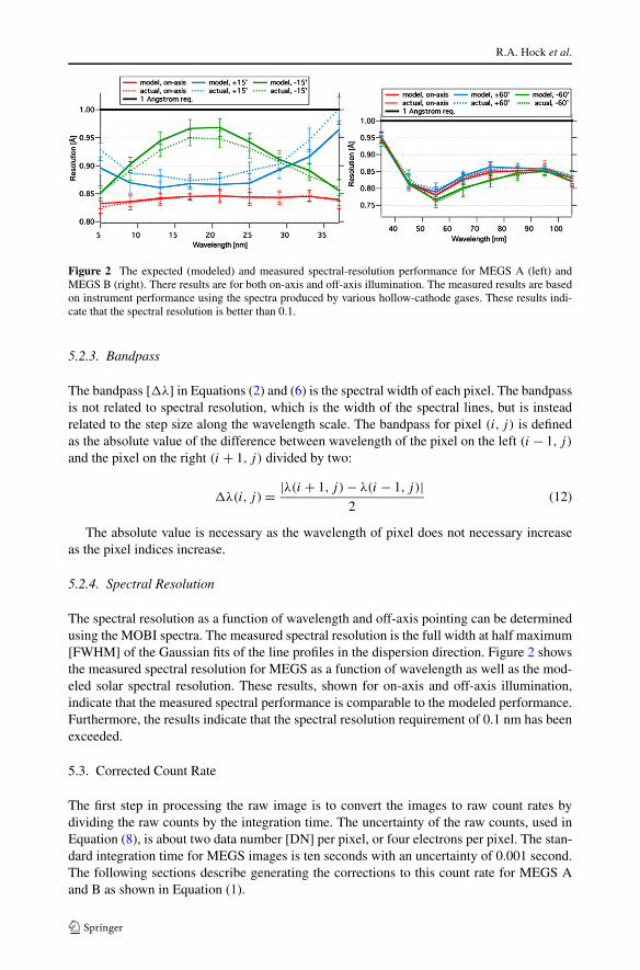
Figure 2 The expected (modeled) and measured spectral-resolution performance for MEGS A (left) andMEGS B (right). There results are for both on-axis and off-axis illumination. The measured results are basedon instrument performance using the spectra produced by various hollow-cathode gases. These results indi-cate that the spectral resolution is better than 0.1.
5.2.3. Bandpass
The bandpass [�λ] in Equations (2) and (6) is the spectral width of each pixel. The bandpassis not related to spectral resolution, which is the width of the spectral lines, but is insteadrelated to the step size along the wavelength scale. The bandpass for pixel (i, j) is definedas the absolute value of the difference between wavelength of the pixel on the left (i − 1, j)
and the pixel on the right (i + 1, j) divided by two:
�λ(i, j) = |λ(i + 1, j) − λ(i − 1, j)|2
(12)
The absolute value is necessary as the wavelength of pixel does not necessary increaseas the pixel indices increase.
5.2.4. Spectral Resolution
The spectral resolution as a function of wavelength and off-axis pointing can be determinedusing the MOBI spectra. The measured spectral resolution is the full width at half maximum[FWHM] of the Gaussian fits of the line profiles in the dispersion direction. Figure 2 showsthe measured spectral resolution for MEGS as a function of wavelength as well as the mod-eled solar spectral resolution. These results, shown for on-axis and off-axis illumination,indicate that the measured spectral performance is comparable to the modeled performance.Furthermore, the results indicate that the spectral resolution requirement of 0.1 nm has beenexceeded.
5.3. Corrected Count Rate
The first step in processing the raw image is to convert the images to raw count rates bydividing the raw counts by the integration time. The uncertainty of the raw counts, used inEquation (8), is about two data number [DN] per pixel, or four electrons per pixel. The stan-dard integration time for MEGS images is ten seconds with an uncertainty of 0.001 second.The following sections describe generating the corrections to this count rate for MEGS Aand B as shown in Equation (1).
Extreme Ultraviolet Variability Experiment (EVE) Multiple EUV
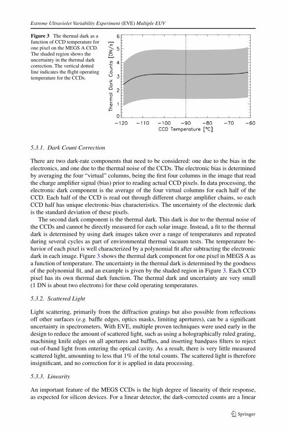
Figure 3 The thermal dark as afunction of CCD temperature forone pixel on the MEGS A CCD.The shaded region shows theuncertainty in the thermal darkcorrection. The vertical dottedline indicates the flight operatingtemperature for the CCDs.
5.3.1. Dark Count Correction
There are two dark-rate components that need to be considered: one due to the bias in theelectronics, and one due to the thermal noise of the CCDs. The electronic bias is determinedby averaging the four “virtual” columns, being the first four columns in the image that readthe charge amplifier signal (bias) prior to reading actual CCD pixels. In data processing, theelectronic dark component is the average of the four virtual columns for each half of theCCD. Each half of the CCD is read out through different charge amplifier chains, so eachCCD half has unique electronic-bias characteristics. The uncertainty of the electronic darkis the standard deviation of these pixels.
The second dark component is the thermal dark. This dark is due to the thermal noise ofthe CCDs and cannot be directly measured for each solar image. Instead, a fit to the thermaldark is determined by using dark images taken over a range of temperatures and repeatedduring several cycles as part of environmental thermal vacuum tests. The temperature be-havior of each pixel is well characterized by a polynomial fit after subtracting the electronicdark in each image. Figure 3 shows the thermal dark component for one pixel in MEGS A asa function of temperature. The uncertainty in the thermal dark is determined by the goodnessof the polynomial fit, and an example is given by the shaded region in Figure 3. Each CCDpixel has its own thermal dark function. The thermal dark and uncertainty are very small(1 DN is about two electrons) for these cold operating temperatures.
5.3.2. Scattered Light
Light scattering, primarily from the diffraction gratings but also possible from reflectionsoff other surfaces (e.g. baffle edges, optics masks, limiting apertures), can be a significantuncertainty in spectrometers. With EVE, multiple proven techniques were used early in thedesign to reduce the amount of scattered light, such as using a holographically ruled grating,machining knife edges on all apertures and baffles, and inserting bandpass filters to rejectout-of-band light from entering the optical cavity. As a result, there is very little measuredscattered light, amounting to less that 1% of the total counts. The scattered light is thereforeinsignificant, and no correction for it is applied in data processing.
5.3.3. Linearity
An important feature of the MEGS CCDs is the high degree of linearity of their response,as expected for silicon devices. For a linear detector, the dark-corrected counts are a linear
R.A. Hock et al.
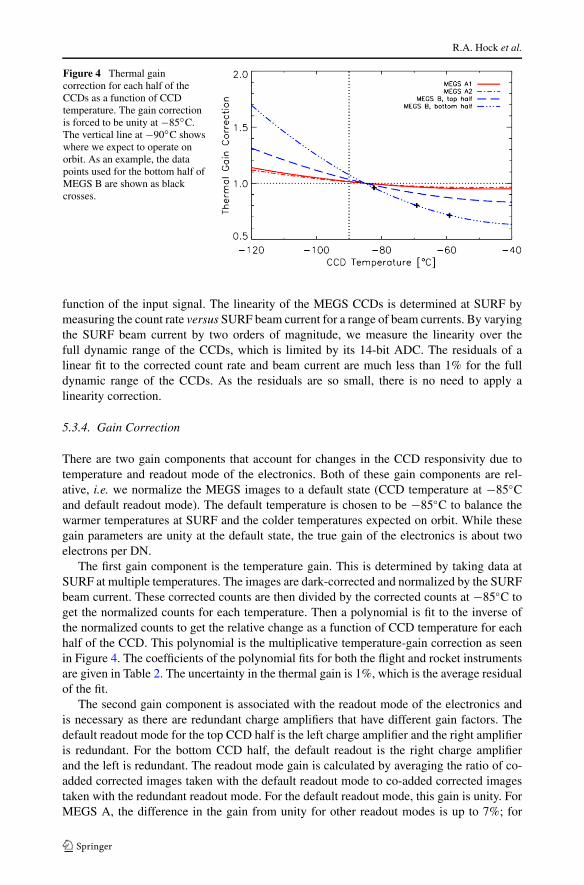
Figure 4 Thermal gaincorrection for each half of theCCDs as a function of CCDtemperature. The gain correctionis forced to be unity at −85◦C.The vertical line at −90◦C showswhere we expect to operate onorbit. As an example, the datapoints used for the bottom half ofMEGS B are shown as blackcrosses.
function of the input signal. The linearity of the MEGS CCDs is determined at SURF bymeasuring the count rate versus SURF beam current for a range of beam currents. By varyingthe SURF beam current by two orders of magnitude, we measure the linearity over thefull dynamic range of the CCDs, which is limited by its 14-bit ADC. The residuals of alinear fit to the corrected count rate and beam current are much less than 1% for the fulldynamic range of the CCDs. As the residuals are so small, there is no need to apply alinearity correction.
5.3.4. Gain Correction
There are two gain components that account for changes in the CCD responsivity due totemperature and readout mode of the electronics. Both of these gain components are rel-ative, i.e. we normalize the MEGS images to a default state (CCD temperature at −85◦Cand default readout mode). The default temperature is chosen to be −85◦C to balance thewarmer temperatures at SURF and the colder temperatures expected on orbit. While thesegain parameters are unity at the default state, the true gain of the electronics is about twoelectrons per DN.
The first gain component is the temperature gain. This is determined by taking data atSURF at multiple temperatures. The images are dark-corrected and normalized by the SURFbeam current. These corrected counts are then divided by the corrected counts at −85◦C toget the normalized counts for each temperature. Then a polynomial is fit to the inverse ofthe normalized counts to get the relative change as a function of CCD temperature for eachhalf of the CCD. This polynomial is the multiplicative temperature-gain correction as seenin Figure 4. The coefficients of the polynomial fits for both the flight and rocket instrumentsare given in Table 2. The uncertainty in the thermal gain is 1%, which is the average residualof the fit.
The second gain component is associated with the readout mode of the electronics andis necessary as there are redundant charge amplifiers that have different gain factors. Thedefault readout mode for the top CCD half is the left charge amplifier and the right amplifieris redundant. For the bottom CCD half, the default readout is the right charge amplifierand the left is redundant. The readout mode gain is calculated by averaging the ratio of co-added corrected images taken with the default readout mode to co-added corrected imagestaken with the redundant readout mode. For the default readout mode, this gain is unity. ForMEGS A, the difference in the gain from unity for other readout modes is up to 7%; for
Extreme Ultraviolet Variability Experiment (EVE) Multiple EUV
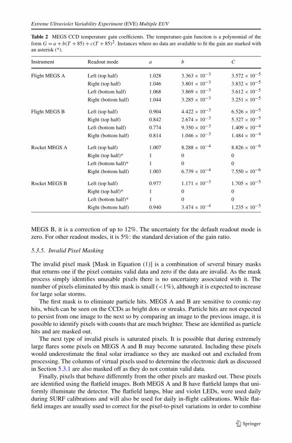
Table 2 MEGS CCD temperature gain coefficients. The temperature-gain function is a polynomial of theform G = a + b(T + 85) + c(T + 85)2. Instances where no data are available to fit the gain are marked withan asterisk (*).
Instrument Readout mode a b C
Flight MEGS A Left (top half) 1.028 3.363 × 10⁻³ 3.572 × 10⁻⁵
Right (top half) 1.046 3.801 × 10⁻³ 3.832 × 10⁻⁵
Left (bottom half) 1.068 3.869 × 10⁻³ 3.612 × 10⁻⁵
Right (bottom half) 1.044 3.285 × 10⁻³ 3.251 × 10⁻⁵
Flight MEGS B Left (top half) 0.904 4.422 × 10⁻³ 6.526 × 10⁻⁵
Right (top half) 0.842 2.674 × 10⁻³ 5.327 × 10⁻⁵
Left (bottom half) 0.774 9.350 × 10⁻³ 1.409 × 10⁻⁴
Right (bottom half) 0.814 1.046 × 10⁻³ 1.484 × 10⁻⁴
Rocket MEGS A Left (top half) 1.007 8.288 × 10⁻⁴ 8.826 × 10⁻⁶
Right (top half)* 1 0 0
Left (bottom half)* 1 0 0
Right (bottom half) 1.003 6.739 × 10⁻⁴ 7.550 × 10⁻⁶
Rocket MEGS B Left (top half) 0.977 1.171 × 10⁻³ 1.705 × 10⁻⁵
Right (top half)* 1 0 0
Left (bottom half)* 1 0 0
Right (bottom half) 0.940 3.474 × 10⁻⁴ 1.235 × 10⁻⁵
MEGS B, it is a correction of up to 12%. The uncertainty for the default readout mode iszero. For other readout modes, it is 5%: the standard deviation of the gain ratio.
5.3.5. Invalid Pixel Masking
The invalid pixel mask [Mask in Equation (1)] is a combination of several binary masksthat returns one if the pixel contains valid data and zero if the data are invalid. As the maskprocess simply identifies unusable pixels there is no uncertainty associated with it. Thenumber of pixels eliminated by this mask is small (<1%), although it is expected to increasefor large solar storms.
The first mask is to eliminate particle hits. MEGS A and B are sensitive to cosmic-rayhits, which can be seen on the CCDs as bright dots or streaks. Particle hits are not expectedto persist from one image to the next so by comparing an image to the previous image, it ispossible to identify pixels with counts that are much brighter. These are identified as particlehits and are masked out.
The next type of invalid pixels is saturated pixels. It is possible that during extremelylarge flares some pixels on MEGS A and B may become saturated. Including these pixelswould underestimate the final solar irradiance so they are masked out and excluded fromprocessing. The columns of virtual pixels used to determine the electronic dark as discussedin Section 5.3.1 are also masked off as they do not contain valid data.
Finally, pixels that behave differently from the other pixels are masked out. These pixelsare identified using the flatfield images. Both MEGS A and B have flatfield lamps that uni-formly illuminate the detector. The flatfield lamps, blue and violet LEDs, were used dailyduring SURF calibrations and will also be used for daily in-flight calibrations. While flat-field images are usually used to correct for the pixel-to-pixel variations in order to combine
R.A. Hock et al.
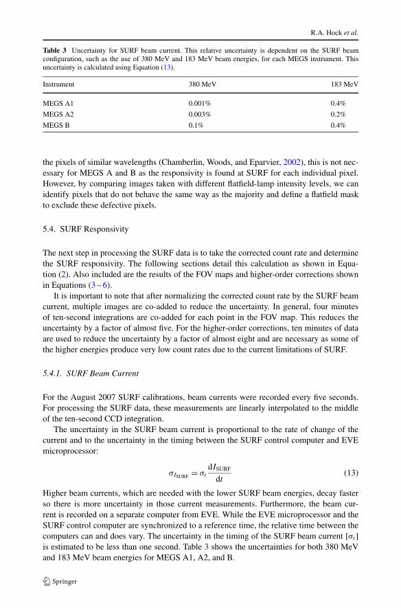
Table 3 Uncertainty for SURF beam current. This relative uncertainty is dependent on the SURF beamconfiguration, such as the use of 380 MeV and 183 MeV beam energies, for each MEGS instrument. Thisuncertainty is calculated using Equation (13).
Instrument 380 MeV 183 MeV
MEGS A1 0.001% 0.4%
MEGS A2 0.003% 0.2%
MEGS B 0.1% 0.4%
the pixels of similar wavelengths (Chamberlin, Woods, and Eparvier, 2002), this is not nec-essary for MEGS A and B as the responsivity is found at SURF for each individual pixel.However, by comparing images taken with different flatfield-lamp intensity levels, we canidentify pixels that do not behave the same way as the majority and define a flatfield maskto exclude these defective pixels.
5.4. SURF Responsivity
The next step in processing the SURF data is to take the corrected count rate and determinethe SURF responsivity. The following sections detail this calculation as shown in Equa-tion (2). Also included are the results of the FOV maps and higher-order corrections shownin Equations (3 – 6).
It is important to note that after normalizing the corrected count rate by the SURF beamcurrent, multiple images are co-added to reduce the uncertainty. In general, four minutesof ten-second integrations are co-added for each point in the FOV map. This reduces theuncertainty by a factor of almost five. For the higher-order corrections, ten minutes of dataare used to reduce the uncertainty by a factor of almost eight and are necessary as some ofthe higher energies produce very low count rates due to the current limitations of SURF.
5.4.1. SURF Beam Current
For the August 2007 SURF calibrations, beam currents were recorded every five seconds.For processing the SURF data, these measurements are linearly interpolated to the middleof the ten-second CCD integration.
The uncertainty in the SURF beam current is proportional to the rate of change of thecurrent and to the uncertainty in the timing between the SURF control computer and EVEmicroprocessor:
σISURF = σt
dISURF
dt(13)
Higher beam currents, which are needed with the lower SURF beam energies, decay fasterso there is more uncertainty in those current measurements. Furthermore, the beam cur-rent is recorded on a separate computer from EVE. While the EVE microprocessor and theSURF control computer are synchronized to a reference time, the relative time between thecomputers can and does vary. The uncertainty in the timing of the SURF beam current [σt ]is estimated to be less than one second. Table 3 shows the uncertainties for both 380 MeVand 183 MeV beam energies for MEGS A1, A2, and B.
Extreme Ultraviolet Variability Experiment (EVE) Multiple EUV
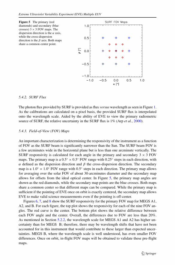
Figure 5 The primary (reddiamonds) and secondary (bluecrosses) 3 × 3 FOV maps. Thedispersion direction is the α axis,while the cross-dispersiondirection is the β axis. Both mapsshare a common center point.
5.4.2. SURF Flux
The photon flux provided by SURF is provided as flux versus wavelength as seen in Figure 1.As the calibrations are calculated on a pixel basis, the provided SURF flux is interpolatedonto the wavelength scale. Aided by the ability of EVE to view the primary radiometricsource of SURF, the relative uncertainty in the SURF flux is 1% (Arp et al., 2000).
5.4.3. Field-of-View (FOV) Maps
An important characterization is determining the responsivity of the instrument as a functionof FOV as the SURF beam is significantly narrower than the Sun. The SURF beam FOV isa few arcminutes wide in the horizontal plane but is less than one arcminute vertically. TheSURF responsivity is calculated for each angle in the primary and secondary 3 × 3 FOVmaps. The primary map is a 0.5◦ × 0.5◦ FOV range with 0.25◦ steps in each direction, withα defined as the dispersion direction and β the cross-dispersion direction. The secondarymap is a 1.0◦ × 1.0◦ FOV range with 0.5◦ steps in each direction. The primary map allowsfor averaging over the solar FOV of about 30-arcminutes diameter and the secondary mapallows for offsets from the ideal optical center. In Figure 5, the primary map angles areshown as the red diamonds, while the secondary map points are the blue crosses. Both mapsshare a common center so that different maps can be compared. While the primary map issufficient if the pointing of EVE once on orbit is exactly centered, the secondary map allowsEVE to make valid science measurements even if the pointing is off-center.
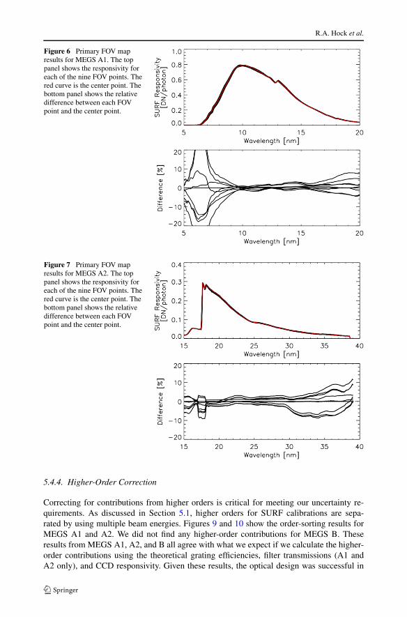
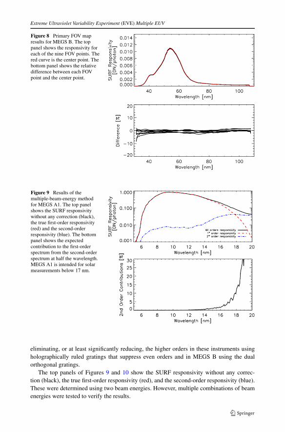
Figures 6, 7, and 8 show the SURF responsivity for the primary FOV map for MEGS A1,A2, and B. For each figure, the top plot shows the responsivity for each of the nine FOV an-gles. The red curve is the center. The bottom plot shows the relative difference betweeneach FOV angle and the center. Overall, the differences due to FOV are less than 20%.As mentioned in Section 5.2.2, the wavelength scale for MEGS A1 and A2 has higher un-certainty than for MEGS B; therefore, there may be wavelength shifts that have not beenaccounted for in this instrument that would contribute to these larger than expected uncer-tainties. MEGS B, where the wavelength scale is well understood, has even smaller FOVdifferences. Once on orbit, in-flight FOV maps will be obtained to validate these pre-flightmaps.
R.A. Hock et al.
Figure 6 Primary FOV mapresults for MEGS A1. The toppanel shows the responsivity foreach of the nine FOV points. Thered curve is the center point. Thebottom panel shows the relativedifference between each FOVpoint and the center point.
Figure 7 Primary FOV mapresults for MEGS A2. The toppanel shows the responsivity foreach of the nine FOV points. Thered curve is the center point. Thebottom panel shows the relativedifference between each FOVpoint and the center point.
5.4.4. Higher-Order Correction
Correcting for contributions from higher orders is critical for meeting our uncertainty re-quirements. As discussed in Section 5.1, higher orders for SURF calibrations are sepa-rated by using multiple beam energies. Figures 9 and 10 show the order-sorting results forMEGS A1 and A2. We did not find any higher-order contributions for MEGS B. Theseresults from MEGS A1, A2, and B all agree with what we expect if we calculate the higher-order contributions using the theoretical grating efficiencies, filter transmissions (A1 andA2 only), and CCD responsivity. Given these results, the optical design was successful in
Extreme Ultraviolet Variability Experiment (EVE) Multiple EUV
Figure 8 Primary FOV mapresults for MEGS B. The toppanel shows the responsivity foreach of the nine FOV points. Thered curve is the center point. Thebottom panel shows the relativedifference between each FOVpoint and the center point.
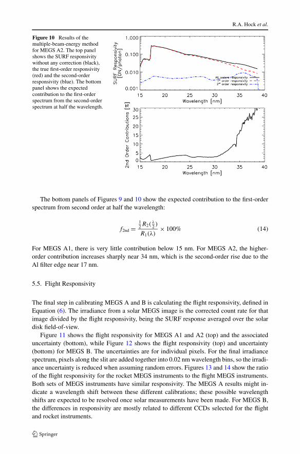
Figure 9 Results of themultiple-beam-energy methodfor MEGS A1. The top panelshows the SURF responsivitywithout any correction (black),the true first-order responsivity(red) and the second-orderresponsivity (blue). The bottompanel shows the expectedcontribution to the first-orderspectrum from the second-orderspectrum at half the wavelength.MEGS A1 is intended for solarmeasurements below 17 nm.
eliminating, or at least significantly reducing, the higher orders in these instruments usingholographically ruled gratings that suppress even orders and in MEGS B using the dualorthogonal gratings.
The top panels of Figures 9 and 10 show the SURF responsivity without any correc-tion (black), the true first-order responsivity (red), and the second-order responsivity (blue).These were determined using two beam energies. However, multiple combinations of beamenergies were tested to verify the results.
R.A. Hock et al.
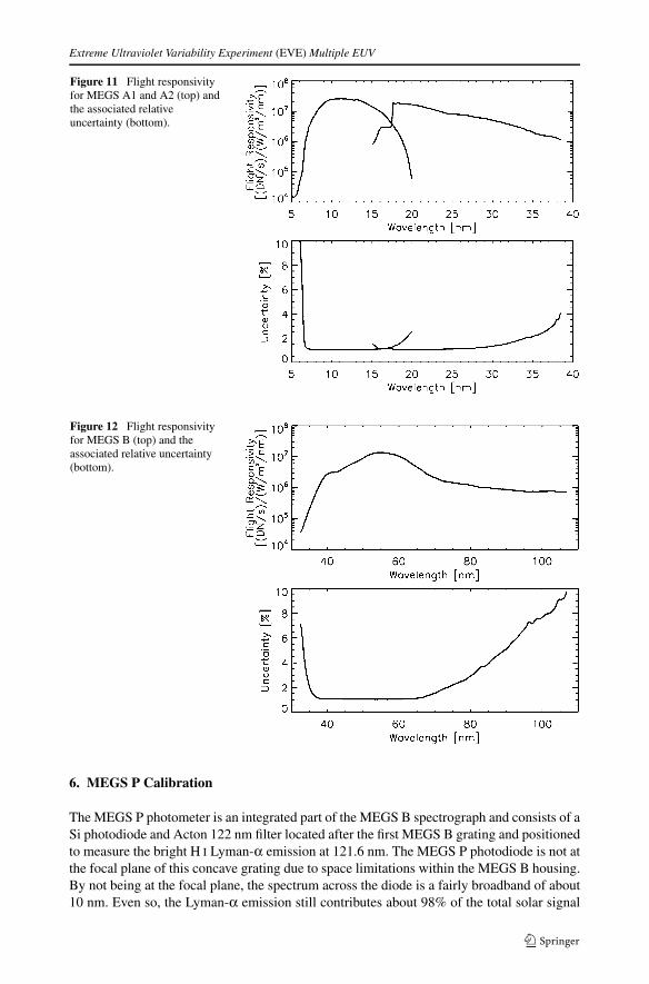
Figure 10 Results of themultiple-beam-energy methodfor MEGS A2. The top panelshows the SURF responsivitywithout any correction (black),the true first-order responsivity(red) and the second-orderresponsivity (blue). The bottompanel shows the expectedcontribution to the first-orderspectrum from the second-orderspectrum at half the wavelength.
The bottom panels of Figures 9 and 10 show the expected contribution to the first-orderspectrum from second order at half the wavelength:
f2nd =12R2(
λ2 )
R1(λ)× 100% (14)
For MEGS A1, there is very little contribution below 15 nm. For MEGS A2, the higher-order contribution increases sharply near 34 nm, which is the second-order rise due to theAl filter edge near 17 nm.
5.5. Flight Responsivity
The final step in calibrating MEGS A and B is calculating the flight responsivity, defined inEquation (6). The irradiance from a solar MEGS image is the corrected count rate for thatimage divided by the flight responsivity, being the SURF response averaged over the solardisk field-of-view.
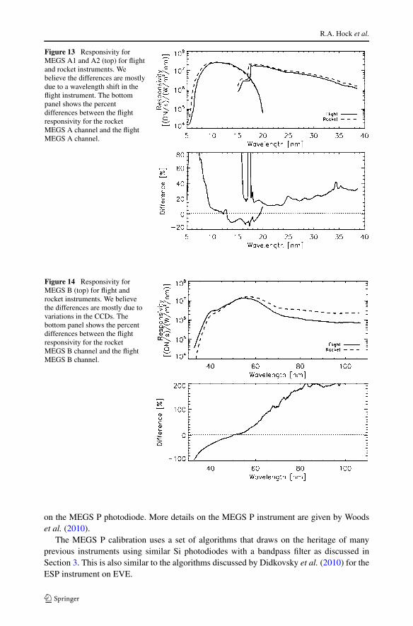
Figure 11 shows the flight responsivity for MEGS A1 and A2 (top) and the associateduncertainty (bottom), while Figure 12 shows the flight responsivity (top) and uncertainty(bottom) for MEGS B. The uncertainties are for individual pixels. For the final irradiancespectrum, pixels along the slit are added together into 0.02 nm wavelength bins, so the irradi-ance uncertainty is reduced when assuming random errors. Figures 13 and 14 show the ratioof the flight responsivity for the rocket MEGS instruments to the flight MEGS instruments.Both sets of MEGS instruments have similar responsivity. The MEGS A results might in-dicate a wavelength shift between these different calibrations; these possible wavelengthshifts are expected to be resolved once solar measurements have been made. For MEGS B,the differences in responsivity are mostly related to different CCDs selected for the flightand rocket instruments.
Extreme Ultraviolet Variability Experiment (EVE) Multiple EUV
Figure 11 Flight responsivityfor MEGS A1 and A2 (top) andthe associated relativeuncertainty (bottom).
Figure 12 Flight responsivityfor MEGS B (top) and theassociated relative uncertainty(bottom).
6. MEGS P Calibration
The MEGS P photometer is an integrated part of the MEGS B spectrograph and consists of aSi photodiode and Acton 122 nm filter located after the first MEGS B grating and positionedto measure the bright H I Lyman-α emission at 121.6 nm. The MEGS P photodiode is not atthe focal plane of this concave grating due to space limitations within the MEGS B housing.By not being at the focal plane, the spectrum across the diode is a fairly broadband of about10 nm. Even so, the Lyman-α emission still contributes about 98% of the total solar signal
R.A. Hock et al.
Figure 13 Responsivity forMEGS A1 and A2 (top) for flightand rocket instruments. Webelieve the differences are mostlydue to a wavelength shift in theflight instrument. The bottompanel shows the percentdifferences between the flightresponsivity for the rocketMEGS A channel and the flightMEGS A channel.
Figure 14 Responsivity forMEGS B (top) for flight androcket instruments. We believethe differences are mostly due tovariations in the CCDs. Thebottom panel shows the percentdifferences between the flightresponsivity for the rocketMEGS B channel and the flightMEGS B channel.
on the MEGS P photodiode. More details on the MEGS P instrument are given by Woodset al. (2010).
The MEGS P calibration uses a set of algorithms that draws on the heritage of manyprevious instruments using similar Si photodiodes with a bandpass filter as discussed inSection 3. This is also similar to the algorithms discussed by Didkovsky et al. (2010) for theESP instrument on EVE.
Extreme Ultraviolet Variability Experiment (EVE) Multiple EUV
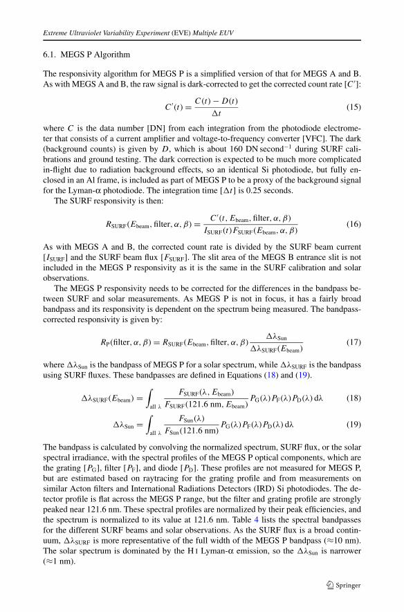
6.1. MEGS P Algorithm
The responsivity algorithm for MEGS P is a simplified version of that for MEGS A and B.As with MEGS A and B, the raw signal is dark-corrected to get the corrected count rate [C ′]:
C ′(t) = C(t) − D(t)
�t(15)
where C is the data number [DN] from each integration from the photodiode electrome-ter that consists of a current amplifier and voltage-to-frequency converter [VFC]. The dark(background counts) is given by D, which is about 160 DN second−1 during SURF cali-brations and ground testing. The dark correction is expected to be much more complicatedin-flight due to radiation background effects, so an identical Si photodiode, but fully en-closed in an Al frame, is included as part of MEGS P to be a proxy of the background signalfor the Lyman-α photodiode. The integration time [�t] is 0.25 seconds.
The SURF responsivity is then:
RSURF(Ebeam,filter, α,β) = C ′(t,Ebeam,filter, α,β)
ISURF(t)FSURF(Ebeam, α,β)(16)
As with MEGS A and B, the corrected count rate is divided by the SURF beam current[ISURF] and the SURF beam flux [FSURF]. The slit area of the MEGS B entrance slit is notincluded in the MEGS P responsivity as it is the same in the SURF calibration and solarobservations.
The MEGS P responsivity needs to be corrected for the differences in the bandpass be-tween SURF and solar measurements. As MEGS P is not in focus, it has a fairly broadbandpass and its responsivity is dependent on the spectrum being measured. The bandpass-corrected responsivity is given by:
RP(filter, α,β) = RSURF(Ebeam,filter, α,β)�λSun
�λSURF(Ebeam)(17)
where �λSun is the bandpass of MEGS P for a solar spectrum, while �λSURF is the bandpassusing SURF fluxes. These bandpasses are defined in Equations (18) and (19).
�λSURF(Ebeam) =∫
all λ
FSURF(λ,Ebeam)
FSURF(121.6 nm,Ebeam)PG(λ)PF(λ)PD(λ)dλ (18)
�λSun =∫
all λ
FSun(λ)
FSun(121.6 nm)PG(λ)PF(λ)PD(λ)dλ (19)
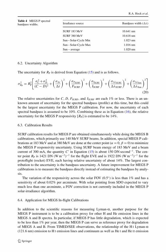
The bandpass is calculated by convolving the normalized spectrum, SURF flux, or the solarspectral irradiance, with the spectral profiles of the MEGS P optical components, which arethe grating [PG], filter [PF], and diode [PD]. These profiles are not measured for MEGS P,but are estimated based on raytracing for the grating profile and from measurements onsimilar Acton filters and International Radiations Detectors (IRD) Si photodiodes. The de-tector profile is flat across the MEGS P range, but the filter and grating profile are stronglypeaked near 121.6 nm. These spectral profiles are normalized by their peak efficiencies, andthe spectrum is normalized to its value at 121.6 nm. Table 4 lists the spectral bandpassesfor the different SURF beams and solar observations. As the SURF flux is a broad contin-uum, �λSURF is more representative of the full width of the MEGS P bandpass (≈10 nm).The solar spectrum is dominated by the H I Lyman-α emission, so the �λSun is narrower(≈1 nm).
R.A. Hock et al.
Table 4 MEGS P spectralbandpass widths. Irradiance source Bandpass width (�λ)
SURF 183 MeV 10.641 nm
SURF 380 MeV 10.618 nm
Sun – Solar-Cycle Min 1.023 nm
Sun – Solar-Cycle Max 1.016 nm
Sun – average 1.020 nm
6.2. Uncertainty Algorithm
The uncertainty for RP is derived from Equation (15) and is as follows.
σ 2RP
= R2P
[σ 2
C +σ 2D
(C − D)2+
(σ�t
�t
)2
+(
σFSURF
FSURF
)2
+(
σISURF
ISURF
)2
+(
σ�λSURF
�λSURF
)2
+(
σ�λSun
�λSun
)2]
(20)
The relative uncertainties for C,D,FSURF, and ISURF are each 1% or less. There is an un-known amount of uncertainty for the spectral bandpass (profile) at this time, but this couldbe the largest uncertainty for the MEGS P calibration. For now, the uncertainty of eachspectral bandpass is assumed to be 10%. Combining these as in Equation (16), the relativeuncertainty for the MEGS P responsivity [RP] is estimated to be 14%.
6.3. Calibration Results
SURF calibration results for MEGS P are obtained simultaneously while doing the MEGS Bcalibrations, which primarily use 140 MeV SURF beams. In addition, special MEGS P cali-brations at 183 MeV and at 380 MeV are done at the center point (α = 0, β = 0) to minimizethe MEGS P responsivity uncertainty. Using SURF beam energy of 183 MeV and a beamcurrent of 300 mA, the quantity C ′ in Equation (15) is about 150 DN second−1. The cen-ter point RP is 1421 DN (W m−2)−1 for the flight EVE and is 1922 DN (W m−2)−1 for theprotoflight (rocket) EVE, each having relative uncertainty of about 14%. The largest con-tribution to the uncertainty is the bandpass uncertainty. A future improvement for MEGS Pcalibrations is to measure the bandpass directly instead of estimating the bandpass by analy-sis.
The variation of the responsivity across the solar FOV (0.5◦) is less than 1% and has asensitivity of about 0.02% per arcminute. With solar pointing from SDO expected to varymuch less than one arcminute, a FOV correction is not currently included in the MEGS Psolar-irradiance algorithm.
6.4. Application for MEGS In-flight Calibrations
In addition to the scientific reasons for measuring Lyman-α, another purpose for theMEGS P instrument is to be a calibration proxy for other H and He emission lines in theMEGS A and B spectra. In particular, if MEGS P has little degradation, which is expectedto be less than 1% per year, then the MEGS P can serve as reference proxy for degradationof MEGS A and B. From TIMED/SEE observations, the relationship of the H I Lyman-α(121.6 nm) emission to H I emission lines and continuum as well as He I and He II emission
Extreme Ultraviolet Variability Experiment (EVE) Multiple EUV
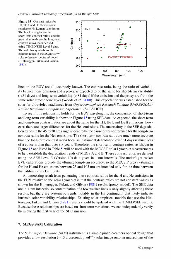
Figure 15 Contrast ratios forH I, He I, and He II emissionsrelative to H I Lyman-α emission.The black triangles are theshort-term contrast ratios, and thegreen diamonds are the long-termcontrast ratios, both derivedusing TIMED/SEE Level 3 data.The red plus symbols are thecontrast ratios in the SC21REFWsolar reference spectrum/model(Hinteregger, Fukui, and Gilson,1981).
lines in the EUV are all accurately known. The contrast ratio, being the ratio of variabil-ity between one emission and a proxy, is expected to be the same for short-term variability(<81 days) and long-term variability (>81 days) if the emission and the proxy are from thesame solar atmospheric layer (Woods et al., 2000). This expectation was established for thesolar far ultraviolet irradiances from Upper Atmosphere Research Satellite (UARS)/SOLarSTellar Irradiance Comparison Experiment (SOLSTICE).
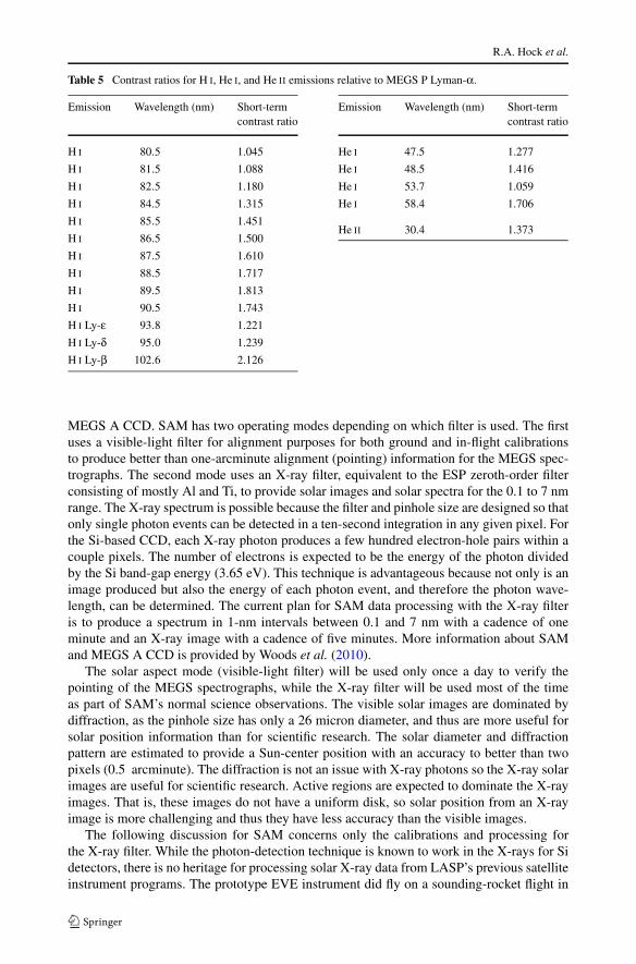
To see if this relationship holds for the EUV wavelengths, the comparison of short-termand long-term variability is shown in Figure 15 using SEE data. As expected, the short-termand long-term contrast ratios are about the same for the H I, He I, and He II emissions; how-ever, there are larger differences for the He I emissions. The uncertainty in the SEE degrada-tion trends in the 45 to 70 nm range appear to be the cause of this difference for the long-termcontrast ratios for the He I emissions. The short-term contrast ratios are much more accuratethan the long-term contrast ratios because instrument degradation over 81 days is much lessof a concern than that over six years. Therefore, the short-term contrast ratios, as shown inFigure 15 and listed in Table 5, will be used with the MEGS P solar Lyman-α measurementsto help establish the degradation trends of MEGS A and B. These contrast ratios are derivedusing the SEE Level 3 (Version 10) data given in 1-nm intervals. The underflight rocketEVE calibrations provide the ultimate long-term accuracy, so the MEGS P proxy estimatesfor the H and He emissions between 25 and 103 nm are intended only for the time betweenthe calibration rocket flights.
An interesting result from generating these contrast ratios for the H and He emissions inthe EUV relative to the solar Lyman-α is that the contrast ratios are not constant values asshown for the Hinteregger, Fukui, and Gilson (1981) results (proxy model). The SEE dataare in 1-nm intervals, so contamination of a few weaker lines is only slightly affecting theseresults, but there are systematic trends, notably in the H I continuum, that likely indicateintrinsic solar-variability relationships. Existing solar empirical models that use the Hin-teregger, Fukui, and Gilson (1981) results should be updated with the TIMED/SEE results.Because these relationships are based on short-term variations, we can independently verifythem during the first year of the SDO mission.
7. MEGS SAM Calibration
The Solar Aspect Monitor (SAM) instrument is a simple pinhole-camera optical design thatprovides a low-resolution (≈15 arcseconds pixel−1) solar image onto an unused part of the
R.A. Hock et al.
Table 5 Contrast ratios for H I, He I, and He II emissions relative to MEGS P Lyman-α.
Emission Wavelength (nm) Short-termcontrast ratio
H I 80.5 1.045
H I 81.5 1.088
H I 82.5 1.180
H I 84.5 1.315
H I 85.5 1.451
H I 86.5 1.500
H I 87.5 1.610
H I 88.5 1.717
H I 89.5 1.813
H I 90.5 1.743
H I Ly-ε 93.8 1.221
H I Ly-δ 95.0 1.239
H I Ly-β 102.6 2.126
Emission Wavelength (nm) Short-termcontrast ratio
He I 47.5 1.277
He I 48.5 1.416
He I 53.7 1.059
He I 58.4 1.706
He II 30.4 1.373
MEGS A CCD. SAM has two operating modes depending on which filter is used. The firstuses a visible-light filter for alignment purposes for both ground and in-flight calibrationsto produce better than one-arcminute alignment (pointing) information for the MEGS spec-trographs. The second mode uses an X-ray filter, equivalent to the ESP zeroth-order filterconsisting of mostly Al and Ti, to provide solar images and solar spectra for the 0.1 to 7 nmrange. The X-ray spectrum is possible because the filter and pinhole size are designed so thatonly single photon events can be detected in a ten-second integration in any given pixel. Forthe Si-based CCD, each X-ray photon produces a few hundred electron-hole pairs within acouple pixels. The number of electrons is expected to be the energy of the photon dividedby the Si band-gap energy (3.65 eV). This technique is advantageous because not only is animage produced but also the energy of each photon event, and therefore the photon wave-length, can be determined. The current plan for SAM data processing with the X-ray filteris to produce a spectrum in 1-nm intervals between 0.1 and 7 nm with a cadence of oneminute and an X-ray image with a cadence of five minutes. More information about SAMand MEGS A CCD is provided by Woods et al. (2010).
The solar aspect mode (visible-light filter) will be used only once a day to verify thepointing of the MEGS spectrographs, while the X-ray filter will be used most of the timeas part of SAM’s normal science observations. The visible solar images are dominated bydiffraction, as the pinhole size has only a 26 micron diameter, and thus are more useful forsolar position information than for scientific research. The solar diameter and diffractionpattern are estimated to provide a Sun-center position with an accuracy to better than twopixels (0.5 arcminute). The diffraction is not an issue with X-ray photons so the X-ray solarimages are useful for scientific research. Active regions are expected to dominate the X-rayimages. That is, these images do not have a uniform disk, so solar position from an X-rayimage is more challenging and thus they have less accuracy than the visible images.
The following discussion for SAM concerns only the calibrations and processing forthe X-ray filter. While the photon-detection technique is known to work in the X-rays for Sidetectors, there is no heritage for processing solar X-ray data from LASP’s previous satelliteinstrument programs. The prototype EVE instrument did fly on a sounding-rocket flight in
Extreme Ultraviolet Variability Experiment (EVE) Multiple EUV
April 2008, so there are some limited solar data during solar-cycle minimum conditions tovalidate the SAM processing algorithms prior to the SDO launch.
7.1. Responsivity Algorithm
The responsivity algorithm for SAM is similar to that of MEGS A, B, and P and is given by:
RSURF(i, j, λ) =∑
all imagesNphotons(i,j,t,λ,Ebeam)
ISURF(t)
FSURF(λ,Ebeam)�tAslit�λ(21)
Here, Nphotons is the number of photon events at a wavelength λ within a band �λ. Toimprove statistics, events from many images are first normalized by the SURF beam currentand then added together. In order to compare the number of photon events measured withthe SURF signal, the SURF flux is multiplied by the integration time [�t]. The slit area[Aslit] is the area of the SAM entrance slit (5.31 × 10⁻¹⁰ cm2). The responsivity [RSURF]consists of the transmission of the Ti – Al – C filter and the quantum throughput [QT] of theCCD. With the CCD QT being almost 100%, the responsivity result is primarily the spectralshape of the filter’s transmission.
Each photon event is assumed to be an isolated event. Double or more concurrent andco-located events, which are intended by design to be less than 10% of the time for solarmaximum conditions, will effectively be treated incorrectly as a single photon event butwith more energy (shorter wavelength). The algorithm to detect a photon event starts byusing a dark- and particle hit-corrected MEGS A image, similar to Equation (1). Then thealgorithm identifies each pixel within the SAM image area that has a signal of greater thanten DN (≈20 electrons). The surrounding pixels with a signal greater than two DN are addedtogether to get the energy of the photon event in DN. This number is then converted to energyunits by multiplying by the gain (GSAM, about two electrons per DN) and the Si band-gapenergy (ESi, 3.65 eV per electron-hole pair). If there are two photon events adjacent to eachother, the algorithm splits the signal of the intermediate pixel between the two events. Eventsthat are larger than 3 × 3 pixels are assumed to contain multiple photon events and are notincluded in the spectrum, although the final spectrum is adjusted to reflect the estimatednumber of events lost in this manner.
Binning by wavelength does not work well for SAM spectra, as a single DN may repre-sent multiple wavelength bins at longer wavelengths or a single wavelength bin may includeseveral DN at shorter wavelengths. Therefore, the SAM spectrum is accumulated in energybins, with each bin equivalent to one DN. In order to create an image, the pixel locationof photons events is recorded and these photon events are accumulated into an image overseveral integrations. With a long enough accumulation period (several minutes to an hour ormore), one could separate the X-ray images into multiple wavelength bands within the 0.1to 7 nm range.
Although the sounding-rocket flight demonstrated the effectiveness of this single-photon-event method for the use with solar data, the SURF calibrations could not properly countenough single photon events for this method to provide accurate results. This shortcomingfor SURF calibrations is due to the SURF beam’s small size, which results in the imagebeing spread over only a couple of pixels (versus hundreds of pixels for a solar image). Asa result, all of the photon events are concentrated in a few pixels, and multiple events aremistakenly counted as higher-energy single events.
R.A. Hock et al.
Therefore, in order to properly calibrate SAM, it was necessary to instead use Equa-tions (22 – 24). The measured signal [Smeasured] in eV second−1 is given by:
Smeasured(t,Ebeam) =∑i,j
Cimage(i, j, t,Ebeam)
�tGSAMESi (22)
where Cimage is the number of DN in each pixel, GSAM the gain to convert DN to electrons,and ESi is energy conversion from electrons to eV (3.65 eV for silicon). The predicted signal[Spredicted] is:
Spredicted(t,Ebeam) =∫ ∞
0RSAM(λ)FSURF(λ,Ebeam)ISURF(t)Aslit dλ (23)
The responsivity of SAM [RSAM] is the transmission model of the Ti – Al – C filter and theCCD detector based on the atomic parameters from Henke, Gullikson, and Davis (1993). Ifthe SAM responsivity is correct, we expect the ratio of Smeasured to Spredicted to be unity. Thisratio represents a scaling factor [fSAM] on how to correct the SAM responsivity.
fSAM(Ebeam) = Smeasured(t,Ebeam)
Spredicted(t,Ebeam)(24)
By using multiple beam energies (331, 361, 380, and 408 MeV), the different scaling fac-tors from each beam energy indicate roughly how the responsivity needs to be adjusted inwavelength. The filter thicknesses were adjusted in the transmission model until fSAM wasnear unity.
The value of the SAM gain factor [GSAM] was determined by using several methods. Theprimary method involved comparing the solar spectrum created from the SAM data whenassuming a gain value of two with the Whole Heliosphere Interval (WHI) solar spectrumgenerated by SORCE/XPS (Woods et al., 2009). A distinct peak in irradiance occurred inboth spectra, but the SAM spectrum had to be shifted to higher energy by a factor of about1.3 in order for these peaks to occur at the same wavelength. This finding suggests thatthe SAM gain factor should have a value of 2.67 e− DN−1. This gain factor, however, onlyapplies to the single-photon-event method used for solar analysis, and does not apply to thesignal integration method because it only registers signals greater than two DN. To get thecorrect gain for SURF calibrations, the signal was extrapolated to determine what the signalwould theoretically be if the limit were set at zero DN. Doing this, the signal would be 7%greater, so the gain value used for SURF calibrations, should be 7% less than for the solarcalibrations, yielding a value of 2.47 e− DN−1.
The spectral-binning method takes advantage of the presence of several solar spectrumlines from the MEGS A2 slit that appear next to the SAM image. The wavelengths of thesespectral lines are known, so therefore the energies of the photon events in these lines are alsoknown. Therefore, the gain can be directly derived from the ratio of the expected photonsignal from a specific wavelength to the measured photon signal. This method generates again value of 3.1 ± 0.44 e− DN−1. On account of the large uncertainty of this method, wedo not use this value for the gain (using instead the 2.47 e− DN−1 from the other method);however, this method does provide limited validation for the other SAM gain values wecalculated.
In order to reflect the actual resolution possible with SAM, we smoothed the responsivitymodel based on the resolution calculated by Equation (25) at each energy before applyingthe model to the solar data. Again, GSAM is the gain factor, while DS is the dark correction
Extreme Ultraviolet Variability Experiment (EVE) Multiple EUV
for the CCD image, and F is the Fano factor, which has a value of 0.115 for silicon. hc/λ
converts wavelength of the photon into energy, while 1/ESi converts energy to number ofelectron-hole pairs. We have
�E = 8.61
√(GSAM
√DS
)2 +(
hc
λ× F
ESi
)(25)
While the SAM X-ray algorithms are developed, they require significantly more valida-tion. This SAM technique for X-ray spectra and images is at an experimental stage. Muchcan be learned from a longer time series of solar observations than what is possible over asingle sounding rocket flight. The SAM results are not a required part of the EVE results, asthe primary source for the 0.1 to 7 nm band is the ESP zeroth-order channel that has the samespectral bandpass as SAM. If the SAM algorithm is found to be properly providing resultsconsistent with the ESP results, then the longer-term degradation for SAM (filter transmis-sion and detector QT) can be tracked with the ESP results. Of particular concern with SAMis the double or more photon events that can contaminate the SAM spectra and images, andhow this contamination might evolve with solar activity (cycle minimum to maximum andduring flares) and with variation in the number of active regions on the solar disk.
7.2. Uncertainty Algorithm
The uncertainty for the SAM responsivity [RSAM] is derived from Equations (22 – 24) andis as follows:
σ 2RSAM
= R2SAM
[(σCimage
Cimage
)2
+(
σ�t
�t
)2
+(
σGSAM
GSAM
)2
+(
σFSURF
FSURF
)2
+(
σISURF
ISURF
)2
+(
σfSAM
fSAM
)2]
(26)
As SAM counts photons, the uncertainty for Cimage is estimated as the square root of Cimage.The uncertainty for the GSAM is about 10%. The relative uncertainties for SURF flux [FSURF]and beam current [ISURF] are both 1.0%. The uncertainty of the scaling factor [σf ] is 0.084.The combination of these uncertainties yields a relative uncertainty of 16% for SAM re-sponsivity.
7.3. Calibration Results
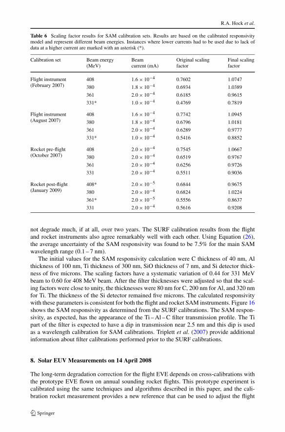
As mentioned in Section 7.1, the SURF calibrations for SAM did not provide reliable photonevents for using Equation (19). Therefore, the SAM responsivity is based on the integratedsignal from the SURF calibrations as described by Equations (22 – 24). In addition to thedata from the calibrations performed at SURF in August 2007, data from a previous SURFcalibration in February 2007 and well as rocket calibrations from October 2007 and January2009 contributed to the calibration process. The data were analyzed using Equation (22)in order to calculate a scaling factor [fSAM]. The responsivity model was then adjustedby altering the filter thicknesses to achieve values for fSAM close to unity. As shown inTable 6, the adjusted responsivity model generated fSAM values that are within 20% of thedesired value. The mean final scaling factor is 0.97 with a standard deviation of 0.084. Theconsistency of the results between the 2007 and 2009 calibrations indicates that SAM did
R.A. Hock et al.
Table 6 Scaling factor results for SAM calibration sets. Results are based on the calibrated responsivitymodel and represent different beam energies. Instances where lower currents had to be used due to lack ofdata at a higher current are marked with an asterisk (*).
Calibration set Beam energy(MeV)
Beamcurrent (mA)
Original scalingfactor
Final scalingfactor
Flight instrument(February 2007)
408 1.6 × 10⁻⁴ 0.7602 1.0747
380 1.8 × 10⁻⁴ 0.6934 1.0389
361 2.0 × 10⁻⁴ 0.6185 0.9615
331* 1.0 × 10−4 0.4769 0.7819
Flight instrument(August 2007)
408 1.6 × 10⁻⁴ 0.7742 1.0945
380 1.8 × 10⁻⁴ 0.6796 1.0181
361 2.0 × 10⁻⁴ 0.6289 0.9777
331* 1.0 × 10−4 0.5416 0.8852
Rocket pre-flight(October 2007)
408 2.0 × 10⁻⁴ 0.7545 1.0667
380 2.0 × 10⁻⁴ 0.6519 0.9767
361 2.0 × 10⁻⁴ 0.6256 0.9726
331 2.0 × 10⁻⁴ 0.5511 0.9036
Rocket post-flight(January 2009)
408* 2.0 × 10−5 0.6844 0.9675
380 2.0 × 10⁻⁴ 0.6824 1.0224
361* 2.0 × 10−5 0.5556 0.8637
331 2.0 × 10⁻⁴ 0.5616 0.9208
not degrade much, if at all, over two years. The SURF calibration results from the flightand rocket instruments also agree remarkably well with each other. Using Equation (26),the average uncertainty of the SAM responsivity was found to be 7.5% for the main SAMwavelength range (0.1 – 7 nm).
The initial values for the SAM responsivity calculation were C thickness of 40 nm, Althickness of 100 nm, Ti thickness of 300 nm, SiO thickness of 7 nm, and Si detector thick-ness of five microns. The scaling factors have a systematic variation of 0.44 for 331 MeVbeam to 0.60 for 408 MeV beam. After the filter thicknesses were adjusted so that the scal-ing factors were close to unity, the thicknesses were 80 nm for C, 200 nm for Al, and 320 nmfor Ti. The thickness of the Si detector remained five microns. The calculated responsivitywith these parameters is consistent for both the flight and rocket SAM instruments. Figure 16shows the SAM responsivity as determined from the SURF calibrations. The SAM respon-sivity, as expected, has the appearance of the Ti – Al – C filter transmission profile. The Tipart of the filter is expected to have a dip in transmission near 2.5 nm and this dip is usedas a wavelength calibration for SAM calibrations. Triplett et al. (2007) provide additionalinformation about filter calibrations performed prior to the SURF calibrations.
8. Solar EUV Measurements on 14 April 2008
The long-term degradation correction for the flight EVE depends on cross-calibrations withthe prototype EVE flown on annual sounding rocket flights. This prototype experiment iscalibrated using the same techniques and algorithms described in this paper, and the cali-bration rocket measurement provides a new reference that can be used to adjust the flight
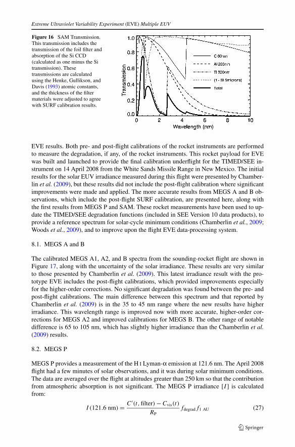
Extreme Ultraviolet Variability Experiment (EVE) Multiple EUV
Figure 16 SAM Transmission.This transmission includes thetransmission of the foil filter andabsorption of the Si CCD(calculated as one minus the Sitransmission). Thesetransmissions are calculatedusing the Henke, Gullikson, andDavis (1993) atomic constants,and the thickness of the filtermaterials were adjusted to agreewith SURF calibration results.
EVE results. Both pre- and post-flight calibrations of the rocket instruments are performedto measure the degradation, if any, of the rocket instruments. This rocket payload for EVEwas built and launched to provide the final calibration underflight for the TIMED/SEE in-strument on 14 April 2008 from the White Sands Missile Range in New Mexico. The initialresults for the solar EUV irradiance measured during this flight were presented by Chamber-lin et al. (2009), but these results did not include the post-flight calibration where significantimprovements were made and applied. The more accurate results from MEGS A and B ob-servations, which include the post-flight SURF calibration, are presented here, along withthe first results from MEGS P and SAM. These rocket measurements have been used to up-date the TIMED/SEE degradation functions (included in SEE Version 10 data products), toprovide a reference spectrum for solar-cycle minimum conditions (Chamberlin et al., 2009;Woods et al., 2009), and to improve upon the flight EVE data-processing system.
8.1. MEGS A and B
The calibrated MEGS A1, A2, and B spectra from the sounding-rocket flight are shown inFigure 17, along with the uncertainty of the solar irradiance. These results are very similarto those presented by Chamberlin et al. (2009). This latest irradiance result with the pro-totype EVE includes the post-flight calibrations, which provided improvements especiallyfor the higher-order corrections. No significant degradation was found between the pre- andpost-flight calibrations. The main difference between this spectrum and that reported byChamberlin et al. (2009) is in the 35 to 45 nm range where the new results have higherirradiance. This wavelength range is improved now with more accurate, higher-order cor-rections for MEGS A2 and improved calibrations for MEGS B. The other range of notabledifference is 65 to 105 nm, which has slightly higher irradiance than the Chamberlin et al.(2009) results.
8.2. MEGS P
MEGS P provides a measurement of the H I Lyman-α emission at 121.6 nm. The April 2008flight had a few minutes of solar observations, and it was during solar minimum conditions.The data are averaged over the flight at altitudes greater than 250 km so that the contributionfrom atmospheric absorption is not significant. The MEGS P irradiance [I ] is calculatedfrom:
I (121.6 nm) = C ′(t,filter) − Cvis(t)
RPfdegradf1 AU (27)
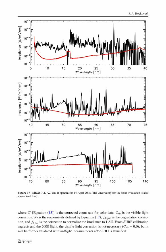
R.A. Hock et al.
Figure 17 MEGS A1, A2, and B spectra for 14 April 2008. The uncertainty for the solar irradiance is alsoshown (red line).
where C ′ [Equation (15)] is the corrected count rate for solar data, Cvis is the visible-lightcorrection, RP is the responsivity defined by Equation (17), fdegrad is the degradation correc-tion, and f1 AU is the correction to normalize the irradiance to 1 AU. From SURF calibrationanalysis and the 2008 flight, the visible-light correction is not necessary (Cvis = 0.0), but itwill be further validated with in-flight measurements after SDO is launched.
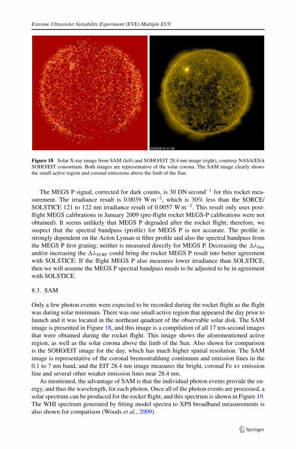
Extreme Ultraviolet Variability Experiment (EVE) Multiple EUV
Figure 18 Solar X-ray image from SAM (left) and SOHO/EIT 28.4 nm image (right), courtesy NASA/ESASOHO/EIT consortium. Both images are representative of the solar corona. The SAM image clearly showsthe small active region and coronal emissions above the limb of the Sun.
The MEGS P signal, corrected for dark counts, is 30 DN second−1 for this rocket mea-surement. The irradiance result is 0.0039 W m−2, which is 30% less than the SORCE/SOLSTICE 121 to 122 nm irradiance result of 0.0057 W m−2. This result only uses post-flight MEGS calibrations in January 2009 (pre-flight rocket MEGS-P calibrations were notobtained). It seems unlikely that MEGS P degraded after the rocket flight; therefore, wesuspect that the spectral bandpass (profile) for MEGS P is not accurate. The profile isstrongly dependent on the Acton Lyman-α filter profile and also the spectral bandpass fromthe MEGS P first grating; neither is measured directly for MEGS P. Decreasing the �λSun
and/or increasing the �λSURF could bring the rocket MEGS P result into better agreementwith SOLSTICE. If the flight MEGS P also measures lower irradiance than SOLSTICE,then we will assume the MEGS P spectral bandpass needs to be adjusted to be in agreementwith SOLSTICE.
8.3. SAM
Only a few photon events were expected to be recorded during the rocket flight as the flightwas during solar minimum. There was one small active region that appeared the day prior tolaunch and it was located in the northeast quadrant of the observable solar disk. The SAMimage is presented in Figure 18, and this image is a compilation of all 17 ten-second imagesthat were obtained during the rocket flight. This image shows the aforementioned activeregion, as well as the solar corona above the limb of the Sun. Also shown for comparisonis the SOHO/EIT image for the day, which has much higher spatial resolution. The SAMimage is representative of the coronal bremsstrahlung continuum and emission lines in the0.1 to 7 nm band, and the EIT 28.4 nm image measures the bright, coronal Fe xv emissionline and several other weaker emission lines near 28.4 nm.
As mentioned, the advantage of SAM is that the individual photon events provide the en-ergy, and thus the wavelength, for each photon. Once all of the photon events are processed, asolar spectrum can be produced for the rocket flight, and this spectrum is shown in Figure 19.The WHI spectrum generated by fitting model spectra to XPS broadband measurements isalso shown for comparison (Woods et al., 2009).
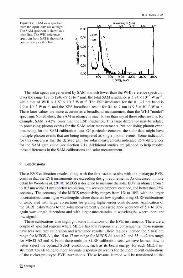
R.A. Hock et al.
Figure 19 SAM solar spectrumfrom the April 2008 rocket flight.The SAM spectrum is shown as athick line. The WHI referencespectrum from XPS is shown forcomparison as a thin line.
The solar spectrum generated by SAM is much lower than the WHI reference spectrum.Over the range 177 to 1240 eV (1 to 7 nm), the total SAM irradiance is 5.74 × 10⁻⁵ W m−2,while that of WHI is 1.57 × 10⁻⁴ W m−2. The ESP irradiance for the 0.1 – 7 nm band is9.9 × 10−5 W m−2, and the XPS broadband result for 0.1 to 7 nm is 9.3 × 10⁻⁵ W m−2.These later values are more accurate as a broadband measurement than the WHI “model”spectrum. Nonetheless, the SAM irradiance is much lower than any of these other results; forexample, SAM is 42% lower than the ESP irradiance. This large difference may be relatedto processing photon events for the SAM solar measurements, but not doing photon eventprocessing for the SAM calibration data. Of particular concern, the solar data might havemultiple photon events that are being interpreted as single photon events. Some indicationfor this concern is that the derived gain for solar measurements indicated 25% differencesfor the SAM gain value (see Section 7.1). Additional studies are planned to help resolvethese differences in the SAM calibrations and solar measurement.
9. Conclusions
These EVE calibration results, along with the first rocket results with the prototype EVE,confirm that the EVE instruments are exceeding design requirements. As discussed in moredetail by Woods et al. (2010), MEGS is designed to measure the solar EUV irradiance from 5to 105 nm with 0.1 nm spectral resolution, ten-second temporal cadence, and better than 25%accuracy. The accuracy of the MEGS responsivity ranges from 1% to 10%, with the largeruncertainties occurring at wavelengths where there are low signals during SURF calibrationsor associated with larger corrections for grating higher-order contributions. Application ofthe SURF calibrations to the solar measurement yields irradiance accuracy of 5% to 20%,again wavelength dependent and with larger uncertainties at wavelengths where there arelow signals.
These calibrations also highlight some limitations of the EVE instruments. There are acouple of spectral regions where MEGS has low responsivity; consequently, those regionshave less accurate calibration and irradiance results. These regions include the 5 to 6 nmrange for MEGS A1, the 15 to 17 nm range for MEGS A1 and A2, and 35 to 42 nm rangefor MEGS A2 and B. From these multiple SURF calibration sets, we have learned how tobetter select the optimal SURF conditions, such as its beam energy, for each MEGS in-strument, thus leading to more accurate responsivity results for the more recent calibrationsof the rocket-prototype EVE instruments. These lessons learned will be transferred to the
Extreme Ultraviolet Variability Experiment (EVE) Multiple EUV
flight EVE with the first EVE underflight rocket calibration, planned for three months afterSDO launches. The MEGS P spectral bandpass is the least accurate part of its algorithm,estimated to have 10% uncertainty but perhaps larger. Overlap with SOLSTICE can pro-vide in-flight calibration for MEGS P to improve upon its pre-flight calibrations. The SAMsolar-irradiance results have significant differences between its spectrum and the modeledspectrum used in the analysis of XPS broadband data. Some of this difference could be re-lated to the model predictions, but part of this difference might be related to the photon eventextraction algorithm. More extended measurements, than just one rocket measurement, areexpected to help clarify the differences and lead to improvements for the SAM calibrationsand algorithms.
The results from EVE, along with the solar-cycle minimum results from the rocket launchin April 2008, will significantly improve upon the understanding of the solar EUV variabil-ity over all time scales from solar-cycle variations over a period of years, to solar-rotationvariations that happen on the order of days, as well as solar flares on time scales of sec-onds to hours. The anticipated EVE irradiance results coupled with the solar-imaging resultsfrom SDO’s other experiments will advance our understanding of irradiance variations anderuptive events such as flares. These advances are then expected to improve upon Earth’sionospheric and thermospheric models for space-weather operations, to better track satel-lites, and to manage communication and navigation systems. Furthermore, the EVE obser-vations will provide an important extension of the solar EUV irradiance record currentlybeing made by the SOHO and TIMED satellites.
Acknowledgements The authors would like to express their appreciation to Mitch Furst and the staff atNIST SURF III for all of their help throughout this calibration process, and special thanks go to Mitch Furstfor reviewing this paper. We would also like to thank the many dedicated LASP scientists and engineerswho designed and built EVE, and the many who also spent many weeks at the NIST calibration facility toobtain these calibration results. We also express special thanks to Vanessa George at LASP for supporting thepreparation of this manuscript. We thank the referee for their helpful comments and suggestions. The solarirradiance results from 14 April 2008 can be obtained from the LASP Interactive Solar Irradiance Datacenter(LISIRD, http://lasp.colorado.edu/lisird). The EIT image is from the SOHO/EIT Consortium; SOHO is a jointESA and NASA program. This research is supported by NASA contract NAS5-02140.
Open Access This article is distributed under the terms of the Creative Commons Attribution Noncommer-cial License which permits any noncommercial use, distribution, and reproduction in any medium, providedthe original author(s) and source are credited.
References
Arp, U., Friedman, R., Furst, M.L., Makar, S., Shaw, P.-S.: 2000, Metrologia 37, 357.Bailey, S.M., Woods, T.N., Eparvier, F.G., Solomon, S.C.: 2006, Adv. Space Res. 37, 209.Chamberlin, P.C., Woods, T.N., Eparvier, F.G.: 2002, Opt. Eng. 45, 063605.Chamberlin, P.C., Hock, R.A., Crotser, D.A., Eparvier, F.G., Furst, M., Triplett, M.A., Woodraska, D., Woods,
T.N.: 2007, SPIE Proc. 6689, 66890N.Chamberlin, P.C., Woods, T.N., Crotser, D.A., Eparvier, F.G., Hock, R.A., Woodraska, D.L.: 2009, Geophys.
Res. Lett. 36, L05102.Crotser, D.A., Woods, T.N., Eparvier, F.G., Ucker, G., Kohnert, R., Berthiaume, G., Weitz, D.: 2004, SPIE
Proc. 5563, 182.Crotser, D.A., Woods, T.N., Eparvier, F.G., Triplett, M.A., Woodraska, D.L.: 2007, SPIE Proc. 6689,
66890M.Didkovsky, L., Judge, D., Wieman, S., Woods, T., Jones, A.: 2010, Solar Phys. doi:10.1007/s11207-009-
9485-8.Henke, B.L., Gullikson, E.M., Davis, J.C.: 1993, At. Data Nucl. Data Tables 54, 181.Hinteregger, H.E., Fukui, K., Gilson, B.R.: 1981, Geophys. Res. Lett. 8, 1147.

R.A. Hock et al.
Rottman, G.J., Woods, T.N., Sparn, T.P.: 1993, J. Geophys. Res. 98, 10667.Saloman, E.B.: 1975, Appl. Opt. 14, 1391.Triplett, M.A., Crotser, D.A., Woods, T.N., Eparvier, F.G., Chamberlin, P.C., Berthiaume, G.D., Weitz, D.M.,
Vest, R.E.: 2007, SPIE Proc. 6689, 668900.Westhoff, R.C., Rose, M.K., Gregory, J.A., Berthiaume, G.D., Seely, J.F., Woods, T.N., Ucker, G.: 2007,
SPIE Proc. 6686, 668604.Woods, T.N., Rottman, G.: 2005, Solar Phys. 230, 375.Woods, T.N., Rottman, G., Vest, R.: 2005, Solar Phys. 230, 345.Woods, T.N., Tobiska, W.K., Rottman, G.J., Worden, J.R.: 2000, J. Geophys. Res. 105, 27195.Woods, T.N., Eparvier, F.G., Bailey, S.M., Chamberlin, P.C., Lean, J., Rottman, G.J., Solomon, S.C., Tobiska,
W.K., Woodraska, D.L.: 2005, J. Geophys. Res. 110, A01312.Woods, T.N., Chamberlin, P.C., Harder, J.W., Hock, R.A., Snow, M., Eparvier, F.G., Fontenla, J., McClintock,
W.E., Richard, E.C.: 2009, Geophys. Res. Lett. 36, L01101.Woods, T.N., Chamberlin, P., Eparvier, F.G., Hock, R., Jones, A., Woodraska, D., Judge, D., Didkosky, L.,
Lean, J., Mariska, J., McMullin, D., Warren, H., Berthiaume, G., Bailey, S., Fuller-Rowell, T., Sojka, J.,Tobiska, W.K., Viereck, R.: 2010, Solar Phys. doi:10.1007/s11207-009-9487-6.


![LEAST SQUARES REGRESSION · 6 Interpretation: [Picture] SYY = ∑ (yi - y )2 is a measure of the total variability of the y i's from y . RSS = ∑ ! e ö i 2 is a measure of the variability](https://static.fdocument.org/doc/165x107/5e749a54162db740442a15f9/least-squares-regression-6-interpretation-picture-syy-a-yi-y-2-is-a-measure.jpg)