( ) ( )*

2,1 1,2 2,1 1 21,2 0 12

1 2 1

1 +(1- ) cos( ) /sin e

1 cos

E E E B α TE TS = ρ B α

E E B α

−−−

[1]

( )1

2 2202 1 1

B1 2

a d cσ T B Bσ = +

N S S

⎡ ⎤⎛ ⎞ ⎛ ⎞∂ ∂⎢ ⎥⎜ ⎟ ⎜ ⎟∂ ∂⎢ ⎥⎝ ⎠ ⎝ ⎠⎣ ⎦

[2]

TR1

TR2

TR1

TR2

αα α

ACQ ACQ

Fig. 1. Schematic representation of the pulse sequence. Images are acquired after each excitation using EPI readouts. Flip angle and TRs are chosen to optimize precision of B1 estimation per unit time (normalized error). See Fig.2.

0 0.002 0.004 0.006 0.008 0.010

100

200

300

400

500

600

σB1

AFITROMBONE

x6 better

0.7 0.8 0.9 1 1.1 1.20.9

0.95

1

1.05

1.1

B1TROMBONE

B1tr

ue/B

1TR

OM

BO

NE

0.7

0.75

0.8

0.85

0.9

0.95

1

1.05

1.1

1.15

0.7

0.75

0.8

0.85

0.9

0.95

1

1.05

1.1

1.15

0.9 0.95 1 1.05 1.10

50

100

150

200

B1TROMBONE / B

1AFI

d e

b ca

Fig. 3. a,b: B1 maps using TROMBONE and AFI methods. c: Histogram of the ratio of B1’s showing that both methods agree to within 1%. d: Histograms of standard deviations of B1 for both methods demonstrating 6-fold improvement in precision. e:Varying T1 within 0.7-4.0 of T1

tune leads to less than ±2.5% deviation from true B1.

0.7 0.8 0.9 1 1.1 1.2

1

2

3

4

5

6

7

8

9

10

B1

ε B1

AFITROMBONE

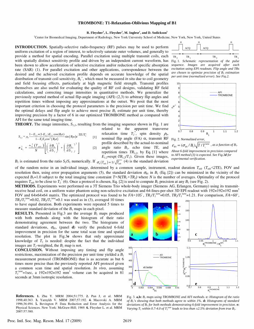
Fig. 2. Normalized error,

11 1 1( / ) / tuneB B B T Tε σ∝ , as a function of B1.

About 6-fold improvement in precision compared to AFI method (3) is expected. See Fig.3d for experimental verification.

TROMBONE: T1-Relaxation-Oblivious Mapping of B1

R. Fleysher1, L. Fleysher1, M. Inglese1, and D. Sodickson1 1Center for Biomedical Imaging, Department of Radiology, New York University School of Medicine, New York, New York, United States

INTRODUCTION. Spatially-selective radio-frequency (RF) pulses may be used to perform uniform excitation of a region of interest, to selectively saturate outer volumes, and generally to provide a method for spatial encoding. Parallel excitation using multiple transmit coils, each with spatially distinct sensitivity profile and driven by an independent current waveform, has been shown to allow acceleration of selective excitation and/or reduction of specific absorption rate (SAR) (1). For parallel excitation and other applications, correspondence between the desired and the achieved excitation profile depends on accurate knowledge of the spatial distribution of transmit coil sensitivity, B1

+, which must be measured in situ due to coil geometry and field focusing effects, particularly at high magnetic field strength. Transmit profiles themselves are also useful for evaluating the quality of RF coil designs, validating RF field calculations, and correcting image intensities in quantitative methods. We generalize the previously reported method of actual flip-angle imaging (AFI) (2,3) to arbitrary flip angles and repetition times without imposing any approximations at the outset. We posit that the most important criterion in choosing the protocol parameters is the precision per unit time. We find the optimal delays and flip angle to achieve most precise B1 estimate per unit time, thereby improving precision by a factor of 6 in our optimized TROMBONE method as compared with AFI for the same total imaging time. THEORY. The image intensities, S1,2, resulting from the imaging sequence shown in Fig. 1 are

related to the apparent transverse relaxation time T2

*, spin density ρ�0, nominal flip angle (FA) α, transmit RF profile described by the actual-to-nominal angle ratio B1, echo time TE, and repetition times TR1,2, by Eq. [1] where E1,2=exp(-TR1,2/T1). Given these images,

B1 is estimated from the ratio S2/S1 numerically. If ( )0 1/adc adcT Tσ ∝ (4) is the standard deviation

of the random noise in an individual image, determined by a common sample, instrument, readout duration Tadc (Tadc≤2TE), FOV and resolution then, using error propagation arguments (5), the standard deviation σB1 in B1 (Eq. [2]) can be minimized in the vicinity of the expected B1=1.0 subject to the total imaging time constraint T=N(TR1+TR2) where N is the number of averages. Optimality of the protocol requires Tadc to be close to T2

* (6). Once a protocol is chosen, Eq. [2] is used to compute B1 precision at any B1 (see Fig. 2). METHODS. Experiments were performed on a 3T Siemens Trio whole-body imager (Siemens AG, Erlangen, Germany) using its transmit-receive head coil, on a uniform water phantom using non-selective excitation and 64-lines-per-shot 3D EPI readout with 192×192×192 mm3 FOV and 64×64×64 matrix. The optimized protocol was found to be FA=105○, TR1/T1

tune=0.05, TR2/T1tune=1.21. For comparison, FA=60○,

TR1/T1tune=0.02, TR2/T1

tune=0.1 was used as in (3), averaged 10 times to have equal duration. Both experiments were repeated 5 times to measure standard deviation of the B1 maps in each pixel. RESULTS. Presented in Fig.3 are the average B1 maps produced with both methods along with the histogram of their ratio demonstrating agreement between the two. The histograms of standard deviations, σB1, (panel d) verify the predicted 6-fold improvement in precision for the same total scan time and spatial resolution. The plot in Fig.3e shows that only approximate knowledge of T1 is needed: despite the fact that the individual images are T1-weighted, the B1 map is not. CONCLUSION. Without imposing any timing and flip angle restrictions, maximization of the precision per unit time yielded a B1 measurement protocol (TROMBONE) that is as accurate as but 6 times more precise than the previously reported AFI protocol given a common scan time and spatial resolution. In vivo, assuming T1

tune=1sec, a 192×192×192 mm3 volume can be acquired in 81 seconds at 3mm isotropic resolution.

References. 1. Zhu Y. MRM 2004;51:775. 2. Pan J, et al. MRM 1998;40:363. 3. Yarnykh V. MRM 2007;57:192. 4. Macovski A. MRM 1996;36:494. 5. Bevington P. Data Reduction and Error Analysis for the Physical Sciences. New York: McGraw-Hill; 1969. 6. Fleysher L. et al. MRM 2007;57:380.

Proc. Intl. Soc. Mag. Reson. Med. 17 (2009) 2619