Translations of MATHEMATICAL MONOGRAPHS - …ft-sipil.unila.ac.id/dbooks/Traveling Wave Solutions of...
453
Translations of M ATHEMATICAL M ONOGRAPHS ΑΓΕΩΜΕ ΕΙΣΙΤΩ ΤΡΗΤΟΣ ΜΗ F O U N D E D 1 8 8 8 A M E R I C A N M A T H E M A T I C A L S O C I E T Y American Mathematical Society Providence, Rhode Island Volume 140 Traveling Wave Solutions of Parabolic Systems Aizik I. Volpert Vitaly A. Volpert Vladimir A. Volpert
Transcript of Translations of MATHEMATICAL MONOGRAPHS - …ft-sipil.unila.ac.id/dbooks/Traveling Wave Solutions of...
Translations of
MATHEMATICAL MONOGRAPHS
ΑΓΕ
ΩΜ
Ε
ΕΙΣ
ΙΤΩ
ΤΡΗΤΟΣ ΜΗ
FOUNDED 1888
AM
ER
ICA
N
MATHEMATICAL
SOC
IET
Y
American Mathematical SocietyProvidence, Rhode Island
Volume 140
Traveling Wave Solutions of Parabolic Systems
Aizik I. VolpertVitaly A. VolpertVladimir A. Volpert
A. I. Volpert, Vit. A. Volpert, Vl. A. Volpert
BEGUWIE VOLNY, OPISYVAEMYEPARABOLIQESKIMI SISTEMAMI
Translated by James F. Heyda from an original Russian manuscript
2000 Mathematics Subject Classification. Primary 35K55, 80A30;Secondary 92E10, 80A25.
Abstract. Traveling wave solutions of parabolic systems describe a wide class of phenomena incombustion physics, chemical kinetics, biology, and other natural sciences. The book is devoted tothe general mathematical theory of such solutions. The authors describe in detail such questions asexistence and stability of solutions, properties of the spectrum, bifurcations of solutions, approachof solutions of the Cauchy problem to waves and systems of waves. The final part of the book isdevoted to applications to combustion theory and chemical kinetics.
The book can be used by graduate students and researchers specializing in nonlinear differentialequations, as well as by specialists in other areas (engineering, chemical physics, biology), wherethe theory of wave solutions of parabolic systems can be applied.
Library of Congress Cataloging-in-Publication Data
Vol′pert, A. I. (Aızik Isaakovich)[Begushchie volny, opisyvaemye parabolicheskimi sistemami. English]Traveling wave solutions of parabolic systems/Aizik I. Volpert, Vitaly A. Volpert, Vladimir A.
Volpert.p. cm. — (Translations of mathematical monographs, ISSN 0065-9282; v. 140)
Includes bibliographical references.ISBN 0-8218-4609-4 (acid-free)1. Differential equations, Parabolic. 2. Differential equations, Nonlinear. 3. Chemical
kinetics—Mathematical models. I. Volpert, Vitaly A., 1958– . II. Volpert, Vladimir A., 1954– .III. Title. IV. Series.QA377.V6413 1994515′.353—dc20 94-16518
c© 1994 by the American Mathematical Society. All rights reserved.The American Mathematical Society retains all rightsexcept those granted to the United States Government.
Printed in the United States of America.
Reprinted with corrections, 2000©∞ The paper used in this book is acid-free and falls within the guidelines
established to ensure permanence and durability.Information on copying and reprinting can be found in the back of this volume.
This volume was typeset by the author using AMS-TEX,the American Mathematical Society’s TEX macro system.Visit the AMS home page at URL: http://www.ams.org/
10 9 8 7 6 5 4 3 2 05 04 03 02 01 00
Contents
Preface xi
Introduction. Traveling Waves Described by Parabolic Systems 1§1. Classification of waves 2§2. Existence of waves 11§3. Stability of waves 16§4. Wave propagation speed 22§5. Bifurcations of waves 23§6. Traveling waves in physics, chemistry, and biology 32
Part I. Stationary Waves
Chapter 1. Scalar Equation 39§1. Introduction 39§2. Functionals ω∗ and ω∗ 45§3. Waves and systems of waves 51§4. Properties of solutions of parabolic equations 72§5. Approach to waves and systems of waves 85§6. Supplement (Additions and bibliographic commentaries) 111
Chapter 2. Leray-Schauder Degree 121§1. Introduction. Formulation of results 121§2. Estimate of linear operators from below 128§3. Functional c(u) and operator A(u) 134§4. Leray-Schauder degree 138§5. Linearized operator 141§6. Index of a stationary point 144§7. Supplement. Leray-Schauder degree in the multidimensionalcase 149
Chapter 3. Existence of Waves 153§1. Introduction. Formulation of results 153§2. A priori estimates 159§3. Existence of monotone waves 173§4. Monotone systems 176§5. Supplement and bibliographic commentaries 183
Chapter 4. Structure of the Spectrum 187§1. Elliptic problems with a parameter 189§2. Continuous spectrum 192§3. Structure of the spectrum 198
vii
viii CONTENTS
§4. Examples 208§5. Spectrum of monotone systems 212
Chapter 5. Stability and Approach to a Wave 217§1. Stability with shift and its connection with the spectrum 218§2. Stability of planar waves to spatial perturbations 225§3. Conditions of instability 237§4. Stability of waves for monotone systems 238§5. On the solutions of nonstationary problems 242§6. Approach to a monotone wave 250§7. Minimax representation of the speed 254
Part II. Bifurcation of Waves
Chapter 6. Bifurcation of Nonstationary Modes of Wave Propagation 259§1. Statement of the problem 259§2. Representation of solutions in series form. Stability ofsolutions 263§3. Examples 268
Chapter 7. Mathematical Proofs 273§1. Statement of the problem and linear analysis 273§2. General representation of solutions of the nonlinear problem.Existence of solutions 285§3. Stability of branching-off solutions 295
Part III. Waves in Chemical Kinetics and Combustion
Chapter 8. Waves in Chemical Kinetics 299§1. Equations of chemical kinetics 299§2. Monotone systems 306§3. Existence and stability of waves 312§4. Branching chain reactions 316§5. Other model systems 333
Bibliographic commentaries 335
Chapter 9. Combustion Waves with Complex Kinetics 337§1. Introduction 337§2. Existence of waves for kinetic systems with irreversiblereactions 338§3. Stability of a wave in the case of equality of transportcoefficients 362§4. Examples 366
Bibliographic commentaries 375
Chapter 10. Estimates and Asymptotics of the Speed of CombustionWaves 377
§1. Estimates for the speed of a combustion wave in a condensedmedium 377§2. Estimates for the speed of a gas combustion wave 392§3. Determination of asymptotics of the speed by the method ofsuccessive approximations 400
Bibliographic commentaries 409
CONTENTS ix
Supplement. Asymptotic and Approximate Analytical Methods inCombustion Problems 411
§1. Narrow reaction zone method. Speed of a stationarycombustion wave 411§2. Stability of a stationary combustion wave 415§3. Nonadiabatic combustion 416§4. Stage combustion 418§5. Transformations in a combustion wave 423§6. Application of the methods of bifurcation theory to the studyof nonstationary modes of propagation of combustion waves 426§7. Surveys and monographs 431
Bibliography 433
Preface
The theory of traveling wave solutions of parabolic equations is one of thefast developing areas of modern mathematics. The history of this theory beginswith the famous mathematical work by Kolmogorov, Petrovskiı, and Piskunovand with works in chemical physics, the best known among them by Zel′dovichand Frank-Kamenetskiı in combustion theory and by Semenov, who discoveredbranching chain flames.
Traveling wave solutions are solutions of special type. They can be usuallycharacterized as solutions invariant with respect to translation in space. Theexistence of traveling waves appears to be very common in nonlinear equations,and, in addition, they often determine the behavior of the solutions of Cauchy-typeproblems.
From the physical point of view, traveling waves usually describe transitionprocesses. Transition from one equilibrium to another is a typical case, althoughmore complicated situations can arise. These transition processes usually “forget”their initial conditions and reflect the properties of the medium itself.
Among the basic questions in the theory of traveling waves we mention theproblem of wave existence, stability of waves with respect to small perturbationsand global stability, bifurcations of waves, determination of wave speed, and systemsof waves (or wave trains). The case of a scalar equation has been rather well studied,basically due to applicability of comparison theorems of a special kind for parabolicequations and of phase space analysis for the ordinary differential equations. Forsystems of equations, comparison theorems of this kind are, in general, not appliΓcable, and the phase space analysis becomes much more complicated. This is whysystems of equations are much less understood and require new approaches. Inthis book, some of these approaches are presented, together with more traditionalapproaches adapted for specific classes of systems of equations and for a morecomplete analysis of scalar equations. From our point of view, it is very importantthat these mathematical results find numerous applications, first and foremost inchemical kinetics and combustion. The authors understand that the theory oftraveling waves is far from being complete and hope that this book will help in itsdevelopment.
This book was basically written when the authors worked at the Institute ofChemical Physics of the Soviet Academy of Sciences. This scientific school, createdby N. N. Semenov, Director of the Institute for a long time, by Ya. B. Zeldovich,who worked there, and by other outstanding personalities, has a strong tradition
xi
xii PREFACE
of collaboration among physicists, chemists, and mathematicians. This specialatmosphere had a strong influence on the scientific interests of the authors and wasvery useful to us. We would like to thank all our colleagues with whom we workedfor many years and without whom this book could not have been written.
Aizik VolpertDepartment of Mathematics, Technion, Haifa, 32000, Israel
Vitaly VolpertUniversite Lyon 1, CNRS, Villeurbanne Cedex, 69622 France
Vladimir VolpertNorthwestern University, Evanston, Illinois 60208
June 1993
INTRODUCTION
Traveling Waves Described by Parabolic Systems
Propagation of waves, described by nonlinear parabolic equations, was firstconsidered in a paper by A. N. Kolmogorov, I. G. Petrovskiı, and N. S. Piskunov[Kolm 1]. These mathematical investigations arose in connection with a model forthe propagation of dominant genes, a topic also considered by R. A. Fisher [Fis 1].Moreover, when [Kolm 1] appeared in 1937, the fact that waves can be describednot only by hyperbolic equations, but also by parabolic equations, did not receivethe proper attention of mathematicians. This is indicated by the fact that sub-sequent mathematical papers in this direction (Ya. I. Kanel′ [Kan 1, 2, 3]) didnot appear until more than twenty years later, although mathematical models,which form a basis for these papers, models of combustion, were formulated byYa. B. Zel′dovich somewhat earlier (see, for example, [Zel 4, 5]). It was not untilthe seventies, under the influence of a great number of the most diverse problems ofphysics, chemistry, and biology, that an intensive development of this theme began.
At the present time a large number of papers is devoted to wave solutions ofparabolic systems and this number continues to increase. In recent years, alongwith the study of one-dimensional waves, an interest in multi-dimensional waveshas developed. This interest was stimulated by observation of spinning waves incombustion, spiral waves in chemical kinetics, etc.
The overwhelming number of natural science problems mentioned above leadsto wave solutions of the parabolic system of equations
(0.1)∂u
∂t= A∆u+ F (u),
where u = (u1, . . . , um) is a vector-valued function, A is a symmetric nonnegative-definite matrix, ∆ is the Laplace operator, and F (u) is a given vector-valuedfunction, which we will sometimes refer to as a source. System (0.1) is consideredin a domain Ω of space Rn on whose boundary, assuming Ω does not coincide withRn, boundary conditions are specified.
We attempt in the present introduction to give a general picture of currentresults concerning wave solutions of system (0.1) (see also [Vol 47]). Later on inthe text we present in detail results of a general character, i.e., results connectedwith general methods of analysis and with sufficiently general classes of systems.In the remaining cases we limit ourselves to a brief exposition or to references tooriginal papers. However, in selecting material for a detailed exposition interests ofthe authors are dominant.
Numbering of formulas and various propositions are carried out according tosections, the first digit indicating the section number. If in references the chapter isnot indicated, it may be assumed that reference is being made to a section withinthe current chapter.
1
2 INTRODUCTION. TRAVELING WAVES DESCRIBED BY PARABOLIC SYSTEMS
§1. Classification of waves
Waves described by parabolic systems can be divided into several classes. Themost conventional is the class of waves referred to as stationary. By a stationarywave we mean a solution u(x, t) of system (0.1) of the form
(1.1) u(x, t) = w(x1 − ct, x′),
where w(x) is a function of n variables, x = (x1, . . . , xn), x′ = (x2, . . . , xn), and cis a constant (speed of the wave). We assume here that Ω is a cylinder and thatthe system of coordinates is chosen so that axis x1 is directed along the axis of thecylinder.
In recent years a large body of experimental material has accumulated and, inaddition, a number of mathematical models connected with it have been studiedin which not just stationary waves can be observed. In particular, we can observeperiodic waves , defined as solutions u(x, t) of system (0.1) of the form
(1.2) u(x, t) = w(x1 − ct, x′, t),
where the function w(x, t) is periodic in t; Ω, as defined above, is a cylinder; andx1 is directed along the axis of the cylinder.
Other forms of waves also occur, some of which we indicate below.
1.1. Stationary waves. We present a classification of stationary waves cur-rently being studied. Part I of the present text is devoted to stationary waves.
1.1.1. One-dimensional planar waves. We consider system (0.1) with the fol-lowing boundary condition on the surface of cylinder Ω:
(1.3)∂u
∂ν= 0,
where ν is the normal to the surface. We refer to a solution of the form
(1.4) u(x, t) = w(x1 − ct)
as a planar wave. This, obviously, corresponds to the definition given above of astationary wave, one-dimensional in space, i.e., a solution of the system
(1.5)∂u
∂t= A
∂2u
∂x21+ F (u).
Function w of the variable ξ = x1 − ct is a solution of the following system ofordinary differential equations over the whole axis:
(1.6) Aw′′ + cw′ + F (w) = 0.
Obviously, the system of equations (1.6) can be reduced to the system of first orderequations
(1.7) w′ = p, Ap′ = −cp− F (w).
Thus, the problem of classifying planar waves can be reduced to the study ofthe trajectories of system (1.7). Apparently, however, not all trajectories are ofinterest. Solutions of system (1.6) are stationary solutions of system (1.5), writtenin coordinates connected with the front of a wave; of most interest are those waveswhich are stable stationary solutions.
We present a classification of planar waves encountered in applications.
§1. CLASSIFICATION OF WAVES 3
ξ
c
w
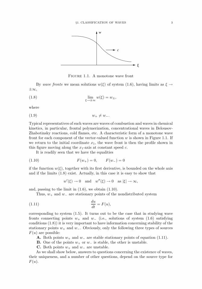
Figure 1.1. A monotone wave front
By wave fronts we mean solutions w(ξ) of system (1.6), having limits as ξ →±∞,
(1.8) limξ→±∞
w(ξ) = w±,
where
(1.9) w+ = w−.
Typical representatives of such waves are waves of combustion and waves in chemicalkinetics, in particular, frontal polymerization, concentrational waves in Belousov-Zhabotinsky reactions, cold flames, etc. A characteristic form of a monotone wavefront for each component of the vector-valued function w is shown in Figure 1.1. Ifwe return to the initial coordinate x1, the wave front is then the profile shown inthis figure moving along the x1-axis at constant speed c.
It is readily seen that we have the equalities
(1.10) F (w+) = 0, F (w−) = 0
if the function w(ξ), together with its first derivative, is bounded on the whole axisand if the limits (1.8) exist. Actually, in this case it is easy to show that
w′(ξ)→ 0 and w′′(ξ)→ 0 as |ξ| → ∞,
and, passing to the limit in (1.6), we obtain (1.10).Thus, w+ and w− are stationary points of the nondistributed system
(1.11)du
dt= F (u),
corresponding to system (1.5). It turns out to be the case that in studying wavefronts connecting points w+ and w− (i.e., solutions of system (1.6) satisfyingconditions (1.8)) it is very important to have information concerning stability of thestationary points w+ and w−. Obviously, only the following three types of sourcesF (u) are possible:
A. Both points w+ and w− are stable stationary points of equation (1.11).B. One of the points w+ or w− is stable, the other is unstable.C. Both points w+ and w− are unstable.As we shall show below, answers to questions concerning the existence of waves,
their uniqueness, and a number of other questions, depend on the source type forF (u).
4 INTRODUCTION. TRAVELING WAVES DESCRIBED BY PARABOLIC SYSTEMS
uw−w+
F
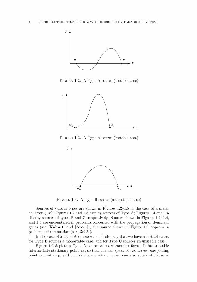
Figure 1.2. A Type A source (bistable case)
F
w+ w− u
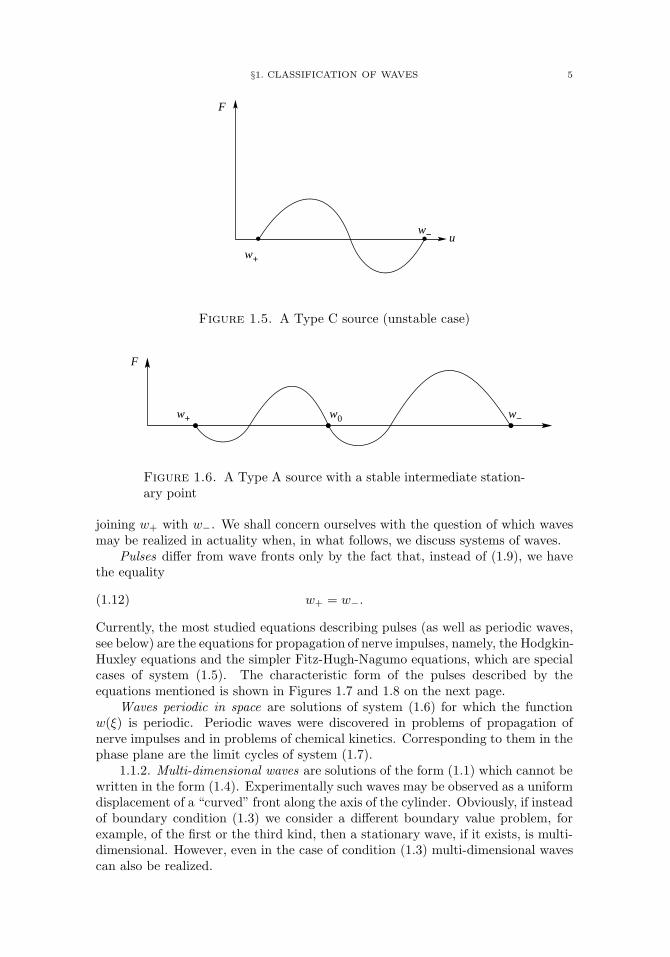
Figure 1.3. A Type A source (bistable case)
F
w+ w−u
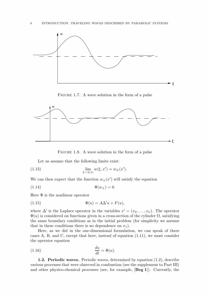
Figure 1.4. A Type B source (monostable case)
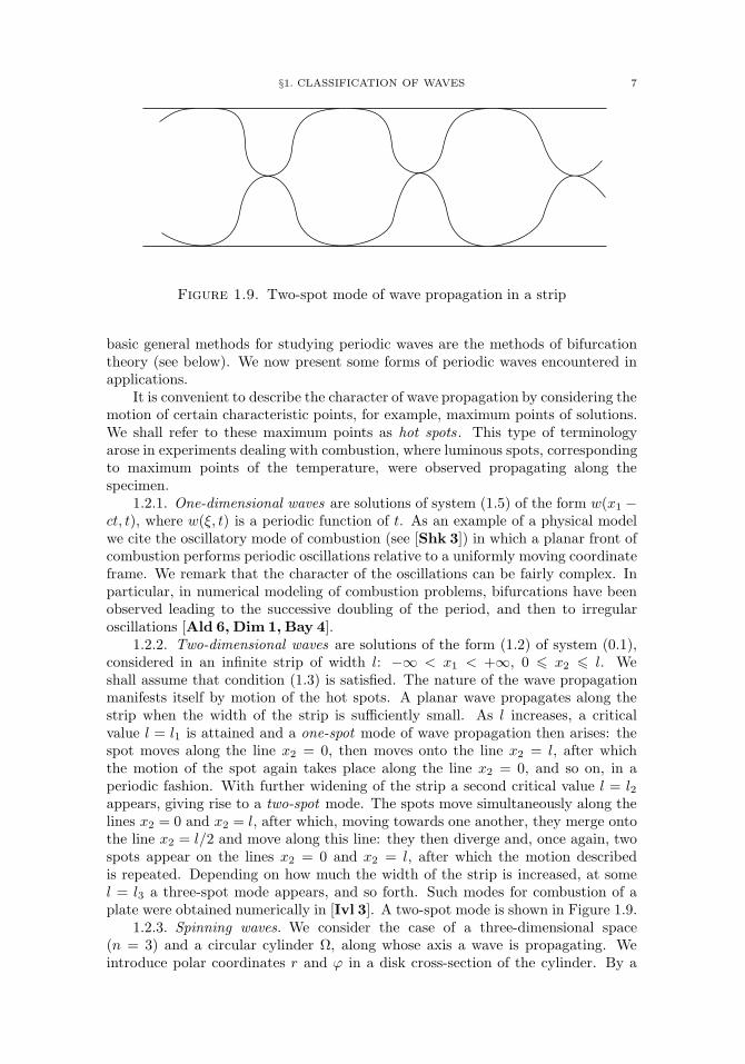
Sources of various types are shown in Figures 1.2–1.5 in the case of a scalarequation (1.5). Figures 1.2 and 1.3 display sources of Type A; Figures 1.4 and 1.5display sources of types B and C, respectively. Sources shown in Figures 1.2, 1.4,and 1.5 are encountered in problems concerned with the propagation of dominantgenes (see [Kolm 1] and [Aro 1]); the source shown in Figure 1.3 appears inproblems of combustion (see [Zel 5]).
In the case of a Type A source we shall also say that we have a bistable case,for Type B sources a monostable case, and for Type C sources an unstable case.
Figure 1.6 depicts a Type A source of more complex form. It has a stableintermediate stationary point w0, so that one can speak of two waves: one joiningpoint w+ with w0, and one joining w0 with w−; one can also speak of the wave
§1. CLASSIFICATION OF WAVES 5
F
w+
w− u
Figure 1.5. A Type C source (unstable case)
F
w+ w−w0
Figure 1.6. A Type A source with a stable intermediate station-ary point
joining w+ with w−. We shall concern ourselves with the question of which wavesmay be realized in actuality when, in what follows, we discuss systems of waves.
Pulses differ from wave fronts only by the fact that, instead of (1.9), we havethe equality
(1.12) w+ = w−.
Currently, the most studied equations describing pulses (as well as periodic waves,see below) are the equations for propagation of nerve impulses, namely, the Hodgkin-Huxley equations and the simpler Fitz-Hugh-Nagumo equations, which are specialcases of system (1.5). The characteristic form of the pulses described by theequations mentioned is shown in Figures 1.7 and 1.8 on the next page.
Waves periodic in space are solutions of system (1.6) for which the functionw(ξ) is periodic. Periodic waves were discovered in problems of propagation ofnerve impulses and in problems of chemical kinetics. Corresponding to them in thephase plane are the limit cycles of system (1.7).
1.1.2. Multi-dimensional waves are solutions of the form (1.1) which cannot bewritten in the form (1.4). Experimentally such waves may be observed as a uniformdisplacement of a “curved” front along the axis of the cylinder. Obviously, if insteadof boundary condition (1.3) we consider a different boundary value problem, forexample, of the first or the third kind, then a stationary wave, if it exists, is multi-dimensional. However, even in the case of condition (1.3) multi-dimensional wavescan also be realized.
6 INTRODUCTION. TRAVELING WAVES DESCRIBED BY PARABOLIC SYSTEMS
w
ξ
Figure 1.7. A wave solution in the form of a pulse
w
ξ
Figure 1.8. A wave solution in the form of a pulse
Let us assume that the following limits exist:
(1.13) limξ→±∞
w(ξ, x′) = w±(x′).
We can then expect that the function w±(x′) will satisfy the equation
(1.14) Φ(w±) = 0.
Here Φ is the nonlinear operator
(1.15) Φ(u) = A∆′u+ F (u),
where ∆′ is the Laplace operator in the variables x′ = (x2, . . . , xn). The operatorΦ(u) is considered on functions given in a cross-section of the cylinder Ω, satisfyingthe same boundary conditions as in the initial problem (for simplicity we assumethat in these conditions there is no dependence on x1).
Here, as we did in the one-dimensional formulation, we can speak of threecases A, B, and C, except that here, instead of equation (1.11), we must considerthe operator equation
(1.16)du
dt= Φ(u).
1.2. Periodic waves. Periodic waves, determined by equation (1.2), describevarious processes that were observed in combustion (see the supplement to Part III)and other physico-chemical processes (see, for example, [Beg 1]). Currently, the
§1. CLASSIFICATION OF WAVES 7
Figure 1.9. Two-spot mode of wave propagation in a strip
basic general methods for studying periodic waves are the methods of bifurcationtheory (see below). We now present some forms of periodic waves encountered inapplications.
It is convenient to describe the character of wave propagation by considering themotion of certain characteristic points, for example, maximum points of solutions.We shall refer to these maximum points as hot spots . This type of terminologyarose in experiments dealing with combustion, where luminous spots, correspondingto maximum points of the temperature, were observed propagating along thespecimen.
1.2.1. One-dimensional waves are solutions of system (1.5) of the form w(x1 −ct, t), where w(ξ, t) is a periodic function of t. As an example of a physical modelwe cite the oscillatory mode of combustion (see [Shk 3]) in which a planar front ofcombustion performs periodic oscillations relative to a uniformly moving coordinateframe. We remark that the character of the oscillations can be fairly complex. Inparticular, in numerical modeling of combustion problems, bifurcations have beenobserved leading to the successive doubling of the period, and then to irregularoscillations [Ald 6, Dim 1, Bay 4].
1.2.2. Two-dimensional waves are solutions of the form (1.2) of system (0.1),considered in an infinite strip of width l: −∞ < x1 < +∞, 0 x2 l. Weshall assume that condition (1.3) is satisfied. The nature of the wave propagationmanifests itself by motion of the hot spots. A planar wave propagates along thestrip when the width of the strip is sufficiently small. As l increases, a criticalvalue l = l1 is attained and a one-spot mode of wave propagation then arises: thespot moves along the line x2 = 0, then moves onto the line x2 = l, after whichthe motion of the spot again takes place along the line x2 = 0, and so on, in aperiodic fashion. With further widening of the strip a second critical value l = l2appears, giving rise to a two-spot mode. The spots move simultaneously along thelines x2 = 0 and x2 = l, after which, moving towards one another, they merge ontothe line x2 = l/2 and move along this line: they then diverge and, once again, twospots appear on the lines x2 = 0 and x2 = l, after which the motion describedis repeated. Depending on how much the width of the strip is increased, at somel = l3 a three-spot mode appears, and so forth. Such modes for combustion of aplate were obtained numerically in [Ivl 3]. A two-spot mode is shown in Figure 1.9.
1.2.3. Spinning waves. We consider the case of a three-dimensional space(n = 3) and a circular cylinder Ω, along whose axis a wave is propagating. Weintroduce polar coordinates r and ϕ in a disk cross-section of the cylinder. By a
8 INTRODUCTION. TRAVELING WAVES DESCRIBED BY PARABOLIC SYSTEMS
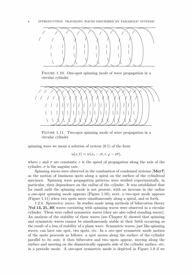
Figure 1.10. One-spot spinning mode of wave propagation in acircular cylinder
Figure 1.11. Two-spot spinning mode of wave propagation in acircular cylinder
spinning wave we mean a solution of system (0.1) of the form
u(x, t) = w(x1 − ct, r, ϕ− σt),
where c and σ are constants; c is the speed of propagation along the axis of thecylinder, σ is the angular rate.
Spinning waves were observed in the combustion of condensed systems [Mer7]as the motion of luminous spots along a spiral on the surface of the cylindricalspecimen. Spinning wave propagation patterns were studied experimentally, inparticular, their dependence on the radius of the cylinder. It was established thatfor small radii the spinning mode is not present; with an increase in the radiusa one-spot spinning mode appears (Figure 1.10); next, a two-spot mode appears(Figure 1.11) when two spots move simultaneously along a spiral, and so forth.
1.2.4. Symmetric waves. In studies made using methods of bifurcation theory[Vol 13, 21, 30] waves coexisting with spinning waves were observed in a circularcylinder. These were called symmetric waves (they are also called standing waves).An analysis of the stability of these waves (see Chapter 6) showed that spinningand symmetric waves cannot be simultaneously stable at their birth occurring asthe result of a loss of stability of a plane wave. Symmetric waves, just like spinningwaves, can have one spot, two spots, etc. In a one-spot symmetric mode motionof the spots proceeds as follows: a spot moves along the surface of the cylinderparallel to its axis; it then bifurcates and two spots appear, moving along thesurface and meeting on the diametrically opposite side of the cylinder surface, etc.in a periodic mode. A one-spot symmetric mode is depicted in Figure 1.9 if we
§1. CLASSIFICATION OF WAVES 9
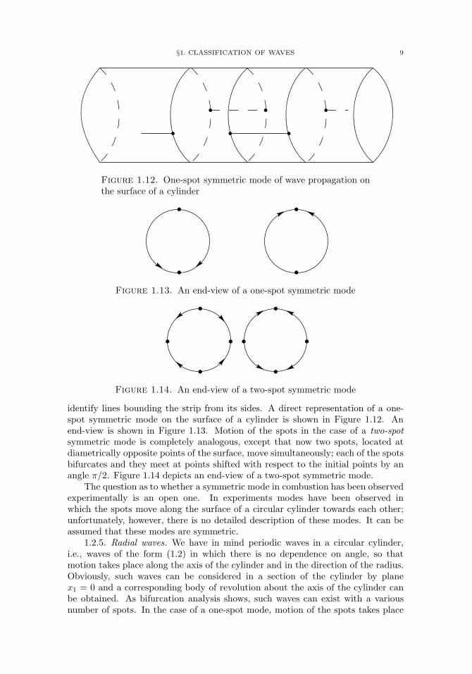
Figure 1.12. One-spot symmetric mode of wave propagation onthe surface of a cylinder
Figure 1.13. An end-view of a one-spot symmetric mode
Figure 1.14. An end-view of a two-spot symmetric mode
identify lines bounding the strip from its sides. A direct representation of a one-spot symmetric mode on the surface of a cylinder is shown in Figure 1.12. Anend-view is shown in Figure 1.13. Motion of the spots in the case of a two-spotsymmetric mode is completely analogous, except that now two spots, located atdiametrically opposite points of the surface, move simultaneously; each of the spotsbifurcates and they meet at points shifted with respect to the initial points by anangle π/2. Figure 1.14 depicts an end-view of a two-spot symmetric mode.
The question as to whether a symmetric mode in combustion has been observedexperimentally is an open one. In experiments modes have been observed inwhich the spots move along the surface of a circular cylinder towards each other;unfortunately, however, there is no detailed description of these modes. It can beassumed that these modes are symmetric.
1.2.5. Radial waves. We have in mind periodic waves in a circular cylinder,i.e., waves of the form (1.2) in which there is no dependence on angle, so thatmotion takes place along the axis of the cylinder and in the direction of the radius.Obviously, such waves can be considered in a section of the cylinder by planex1 = 0 and a corresponding body of revolution about the axis of the cylinder canbe obtained. As bifurcation analysis shows, such waves can exist with a variousnumber of spots. In the case of a one-spot mode, motion of the spots takes place
10 INTRODUCTION. TRAVELING WAVES DESCRIBED BY PARABOLIC SYSTEMS
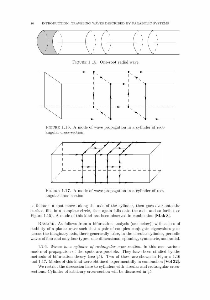
Figure 1.15. One-spot radial wave
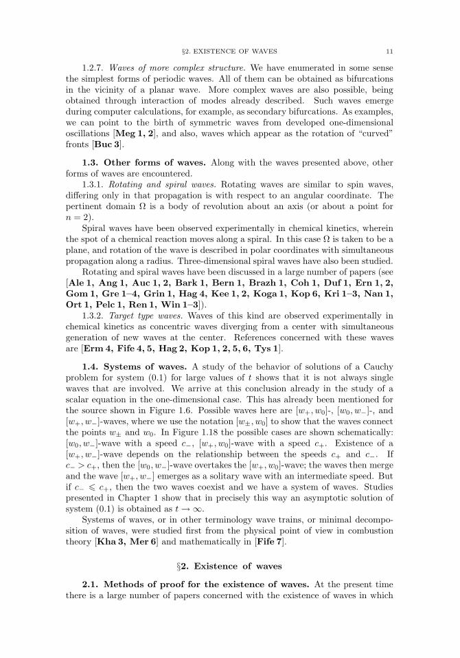
Figure 1.16. A mode of wave propagation in a cylinder of rect-angular cross-section
Figure 1.17. A mode of wave propagation in a cylinder of rect-angular cross-section
as follows: a spot moves along the axis of the cylinder, then goes over onto thesurface, fills in a complete circle, then again falls onto the axis, and so forth (seeFigure 1.15). A mode of this kind has been observed in combustion [Mak 3].
Remark. As follows from a bifurcation analysis (see below), with a loss ofstability of a planar wave such that a pair of complex conjugate eigenvalues goesacross the imaginary axis, there generically arise, in the circular cylinder, periodicwaves of four and only four types: one-dimensional, spinning, symmetric, and radial.
1.2.6. Waves in a cylinder of rectangular cross-section. In this case variousmodes of propagation of the spots are possible. They have been studied by themethods of bifurcation theory (see §5). Two of these are shown in Figures 1.16and 1.17. Modes of this kind were obtained experimentally in combustion [Vol 32].
We restrict the discussion here to cylinders with circular and rectangular cross-sections. Cylinder of arbitrary cross-section will be discussed in §5.
§2. EXISTENCE OF WAVES 11
1.2.7. Waves of more complex structure. We have enumerated in some sensethe simplest forms of periodic waves. All of them can be obtained as bifurcationsin the vicinity of a planar wave. More complex waves are also possible, beingobtained through interaction of modes already described. Such waves emergeduring computer calculations, for example, as secondary bifurcations. As examples,we can point to the birth of symmetric waves from developed one-dimensionaloscillations [Meg 1, 2], and also, waves which appear as the rotation of “curved”fronts [Buc 3].
1.3. Other forms of waves. Along with the waves presented above, otherforms of waves are encountered.
1.3.1. Rotating and spiral waves. Rotating waves are similar to spin waves,differing only in that propagation is with respect to an angular coordinate. Thepertinent domain Ω is a body of revolution about an axis (or about a point forn = 2).
Spiral waves have been observed experimentally in chemical kinetics, whereinthe spot of a chemical reaction moves along a spiral. In this case Ω is taken to be aplane, and rotation of the wave is described in polar coordinates with simultaneouspropagation along a radius. Three-dimensional spiral waves have also been studied.
Rotating and spiral waves have been discussed in a large number of papers (see[Ale 1, Ang 1, Auc 1, 2, Bark 1, Bern 1, Brazh 1, Coh 1, Duf 1, Ern 1, 2,Gom 1, Gre 1–4, Grin 1, Hag 4, Kee 1, 2, Koga 1, Kop 6, Kri 1–3, Nan 1,Ort 1, Pelc 1, Ren 1, Win 1–3]).
1.3.2. Target type waves. Waves of this kind are observed experimentally inchemical kinetics as concentric waves diverging from a center with simultaneousgeneration of new waves at the center. References concerned with these wavesare [Erm 4, Fife 4, 5, Hag 2, Kop 1, 2, 5, 6, Tys 1].
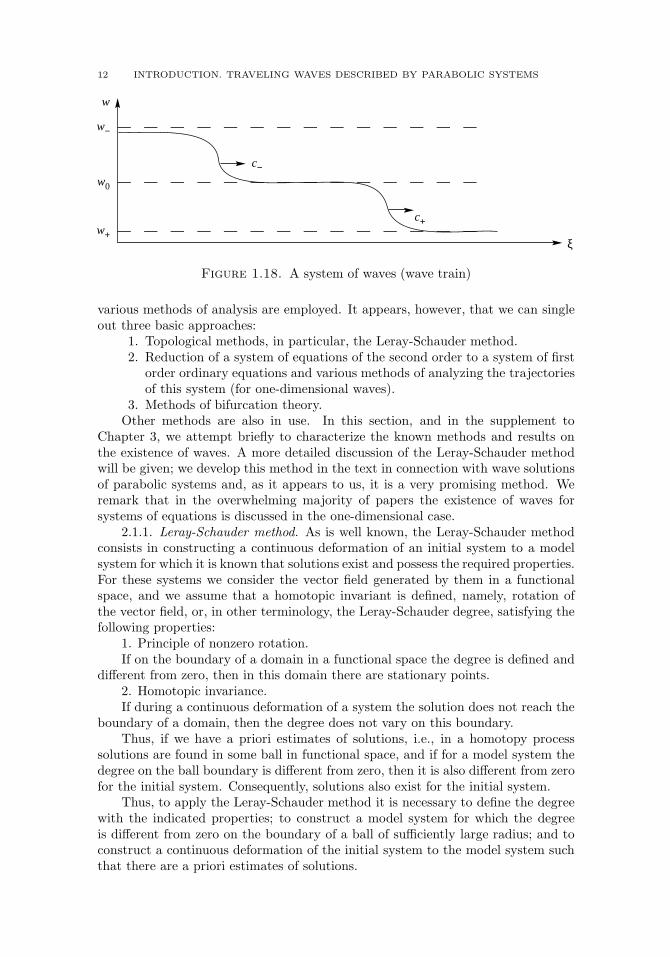
1.4. Systems of waves. A study of the behavior of solutions of a Cauchyproblem for system (0.1) for large values of t shows that it is not always singlewaves that are involved. We arrive at this conclusion already in the study of ascalar equation in the one-dimensional case. This has already been mentioned forthe source shown in Figure 1.6. Possible waves here are [w+, w0]-, [w0, w−]-, and[w+, w−]-waves, where we use the notation [w±, w0] to show that the waves connectthe points w± and w0. In Figure 1.18 the possible cases are shown schematically:[w0, w−]-wave with a speed c−, [w+, w0]-wave with a speed c+. Existence of a[w+, w−]-wave depends on the relationship between the speeds c+ and c−. Ifc− > c+, then the [w0, w−]-wave overtakes the [w+, w0]-wave; the waves then mergeand the wave [w+, w−] emerges as a solitary wave with an intermediate speed. Butif c− c+, then the two waves coexist and we have a system of waves. Studiespresented in Chapter 1 show that in precisely this way an asymptotic solution ofsystem (0.1) is obtained as t→∞.
Systems of waves, or in other terminology wave trains, or minimal decompo-sition of waves, were studied first from the physical point of view in combustiontheory [Kha 3, Mer 6] and mathematically in [Fife 7].
§2. Existence of waves
2.1. Methods of proof for the existence of waves. At the present timethere is a large number of papers concerned with the existence of waves in which
12 INTRODUCTION. TRAVELING WAVES DESCRIBED BY PARABOLIC SYSTEMS
w
w−
w0
w+
c+
c−
ξ
Figure 1.18. A system of waves (wave train)
various methods of analysis are employed. It appears, however, that we can singleout three basic approaches:
1. Topological methods, in particular, the Leray-Schauder method.2. Reduction of a system of equations of the second order to a system of first
order ordinary equations and various methods of analyzing the trajectoriesof this system (for one-dimensional waves).
3. Methods of bifurcation theory.Other methods are also in use. In this section, and in the supplement to
Chapter 3, we attempt briefly to characterize the known methods and results onthe existence of waves. A more detailed discussion of the Leray-Schauder methodwill be given; we develop this method in the text in connection with wave solutionsof parabolic systems and, as it appears to us, it is a very promising method. Weremark that in the overwhelming majority of papers the existence of waves forsystems of equations is discussed in the one-dimensional case.
2.1.1. Leray-Schauder method. As is well known, the Leray-Schauder methodconsists in constructing a continuous deformation of an initial system to a modelsystem for which it is known that solutions exist and possess the required properties.For these systems we consider the vector field generated by them in a functionalspace, and we assume that a homotopic invariant is defined, namely, rotation ofthe vector field, or, in other terminology, the Leray-Schauder degree, satisfying thefollowing properties:
1. Principle of nonzero rotation.If on the boundary of a domain in a functional space the degree is defined and
different from zero, then in this domain there are stationary points.2. Homotopic invariance.If during a continuous deformation of a system the solution does not reach the
boundary of a domain, then the degree does not vary on this boundary.Thus, if we have a priori estimates of solutions, i.e., in a homotopy process
solutions are found in some ball in functional space, and if for a model system thedegree on the ball boundary is different from zero, then it is also different from zerofor the initial system. Consequently, solutions also exist for the initial system.
Thus, to apply the Leray-Schauder method it is necessary to define the degreewith the indicated properties; to construct a model system for which the degreeis different from zero on the boundary of a ball of sufficiently large radius; and toconstruct a continuous deformation of the initial system to the model system suchthat there are a priori estimates of solutions.
§2. EXISTENCE OF WAVES 13
Rotation of a vector field for completely continuous vector fields is well definedand widely applied, in particular, in proving existence of solutions by the Leray-Schauder method. Systems of equations of the type (1.6) can be reduced tocompletely continuous vector fields, but only in case they are considered in boundeddomains (see §1 of Chapter 2). For waves, i.e., for solutions considered in unboundeddomains, one cannot make use of an existing theory for completely continuous vectorfields, and this is actually the case. Essentially the situation is the following.
To construct the degree it is necessary to select, in an appropriate way, afunctional space and to define an operator A vanishing on solutions of system (1.6),i.e., on waves. A vector field will thereby be determined. Operator A can beapproximated in various ways by operators An, which correspond to completelycontinuous vector fields and for which the degree can be defined in the usual way.Moreover, this can be done so that the degree for operators An is independent ofn if n is sufficiently large, and we can take this quantity as the degree of operatorA. If γ(A,D), the degree of operator A on the boundary of domain D, is differentfrom zero, then γ(An, D) will also be different from zero; consequently, there existsa sequence of functions un, belonging to domain D, for which An(un) = 0. Thissequence is bounded (domain D is assumed to be bounded) and, consequently, somesubsequence converges weakly. The main difficulty here is that the weak limit ofthis sequence may not belong to domain D, and, as a consequence, the principleof nonzero rotation can be violated. To avoid this situation we need to show,for the class of operators considered, that weak convergence of solutions impliesstrong convergence (precise statements appear in Chapter 2). To proceed we needto obtain estimates from below for operator A. These estimates for operatorscorresponding to the system of equations (1.6) were obtained, thereby making itpossible to define the degree by Skrypnik’s method [Skr 1]. It should be noted thatrotation of a vector field possessing the usual properties cannot be constructed in anarbitrary functional space. Even in the case of a scalar equation it is easy to give anexample whereby, in the space of continuous functions C, a wave under deformationdisappears with no violation of a priori estimates. This is connected with the factthat during motion with respect to a parameter a wave can be attracted to anintermediate stationary point and, instead of a wave satisfying conditions (1.8), wewill have a system of waves. In constructing the degree for operators describingtraveling waves, it is convenient to use weighted Sobolev spaces.
Yet another difficulty arising here is that solutions of equation (1.6) are invari-ant with respect to a translation in the spatial variable. In addition, the speedc of the wave is an unknown and must also be found in solving the problem. Itis therefore convenient in the study of waves to introduce a functionalization ofthe parameter. This means that the speed of the wave is considered not as anunknown constant, but as a given functional defined on the same space as operatorA. Here the value of the functional depends on the magnitude of the translationof the stationary solution, making it possible to single out one wave from a familyof waves. Thus functionalization of a parameter allows us to consider an isolatedstationary point in a given space instead of a whole line of stationary points.
We remark that the degree for operators describing traveling waves is definedwithout any assumptions as to the form of the nonlinearity of F (u), except, natu-rally, for smoothness and stability of the points w±. This result, apparently, can berather easily generalized to the multi-dimensional case. As for the monostable case,there arise here additional complexities associated with the facts that waves exist
14 INTRODUCTION. TRAVELING WAVES DESCRIBED BY PARABOLIC SYSTEMS
for a whole half-interval (half-axis) of speeds and form an entire family of solutions.It can be expected that the degree can be successfully introduced with a properselection of weighted norms, identifying a single wave (a single speed) of a familyof waves.
Having defined the degree, we see that the possibility of obtaining a prioriestimates of solutions also determines the class of systems for which we can suc-cessfully apply the Leray-Schauder method to prove the existence of waves. (Theconstruction of a model system can be carried out rather easily and is, in the main,of a technical nature.) Hitherto it has been possible to do this for locally-monotonesystems (see §2.2), yet one may expect that there exist other types of nonlinearitiesalso for which a priori estimates of solutions can be obtained. It should be notedthat the problem of obtaining a priori estimates in one form or another also arisesfor other methods of proving the existence of waves; one should therefore not assumethat this restricts the application of the Leray-Schauder method in comparison withother approaches.
2.1.2. Other methods for proving the existence of waves. A widely used me-thod is one based on phase portrait analysis. This means that the system ofequations (1.6) is placed into correspondence with the first order system of equa-tions (1.7). As has already been noted, its trajectories correspond to waves. Inparticular, if the question concerns waves satisfying conditions (1.8), i.e., wavefronts or pulses, we then have in mind trajectories of system (1.7) joining thestationary points (w+, 0) and (w−, 0) in the phase space (w, p). To periodic wavesthere correspond limit cycles.
Thus the problem of proving existence of waves reduces to proving existence ofcorresponding trajectories of system (1.7).
This method is very suitable when applied to a scalar equation. Actually, inthis case (1.7) is a system of two equations and the analysis is carried out in thetwo-dimensional phase plane, a situation rather well studied. To prove existence ofwave fronts a trajectory is drawn off from one of the stationary points (w+, 0) or(w−, 0) and it is proved that the constant c can be selected so that this trajectoryreaches the other of these stationary points. Precisely this method was used for thefirst time in [Kolm 1] to prove the existence of a wave.
The situation is far more involved for the system of equations (1.6). Here itis necessary to consider a phase space of dimensionality greater than or equal to4; application of the method indicated entails essential difficulties. To successfullyapply this method one must deal with a system of special form, possessing specificproperties. It is of interest to note that many systems arising in various physicalproblems possess the required properties. Therefore, it is this approach that wassuccessfully used to prove the existence of wave fronts in various mathematicalmodels of physics, chemistry, and biology (see Chapter 3, §5).
To prove the existence of a pulse, it is obviously sufficient to establish in thephase plane (w, p) the existence of a trajectory of system (1.7) leaving and enteringthe stationary point (w+, 0). In the general case only results obtained with the aidof bifurcation theory are available: under certain conditions birth of a separatrixloop from the stationary points may be proved.
One of the general approaches to proving the existence of periodic waves alsoyields a theory of bifurcations. The question concerns birth of periodic waves ofsmall amplitude from constant stationary solutions under a change of parameters(see below). Another approach to proving the existence of periodic waves is
§2. EXISTENCE OF WAVES 15
connected with an assumption concerning the existence of stable limit cycles forthe system (1.11). Use is made of the small parameter method: for large speeds ca small parameter can be introduced into system (1.6) so that as c→∞ we obtainsystem (1.11).
Results concerning the existence of multi-dimensional waves for scalar equationsare presented in the supplement to Chapter 1. Multi-dimensional waves close toplanar waves have been studied by methods of bifurcation theory (see §5).
2.2. Locally-monotone and monotone systems. Scalar equation. Inthis subsection we present basic results on the existence of waves of wavefront typefor a class of systems of equations. We assume that the matrix A is a diagonalmatrix and that the vector-valued function F (u) satisfies the conditions
(2.1)∂Fi∂uj
0, i, j = 1, . . . , n, i = j,
for all u ∈ Rn. In this case the systems of equations (0.1) and (1.6) are called
monotone systems. Such systems of equations are often encountered in applications(see §6 and Chapters 8 and 9).
The simplest particular case of such systems is the scalar equation (n = 1). Ifconditions (2.1) with strong inequalities are satisfied only on the surfaces Fi(u) = 0(i = 1, . . . , n), the system of equations (0.1) is then said to be locally monotone (ageneralization of this concept is given in §2 of Chapter 3).
As we have already remarked, for wave fronts we assume existence of the lim-its (1.8) and F (w±) = 0. We seek monotone waves (for definiteness, monotonicallydecreasing) with the same direction of monotonicity for all components wi(x) ofthe vector w(x). (Nonmonotone waves for monotone systems are unstable; seeChapter 5, §6.) Obviously, then, w+ < w− and it is sufficient to require thatinequality (2.1) be satisfied in the interval [w+, w−], i.e., for w+ w w−.
We formulate a theorem for the existence of a wave in the case of a source ofType A.
Theorem 2.1. Let system (0.1) be monotone. Further, let the vector-valuedfunction F (u) vanish in a finite number of points uk, w+ uk w− (k = 1, . . . ,m).Let us assume that all the eigenvalues of the matrices F ′(w+) and F ′(w−) lie in theleft half-plane, and that the matrices F ′(uk) (k = 1, . . . ,m) are irreducible and haveat least one eigenvalue in the right half-plane. Then there exists a unique monotonetraveling wave, i.e., a constant c and a twice continuously differentiable monotonevector-valued function w(x) satisfying system (1.6) and the conditions (1.8).
For Type B sources we have the following theorem for the existence of a wave.
Theorem 2.2. Let system (0.1) be monotone. Assume further that the vector-valued function F (u) vanishes at a finite number of points uk, w+ uk w−(k = 1, . . . ,m). Suppose that all eigenvalues of the matrix F ′(w−) lie in the lefthalf-plane and that the matrices F ′(w+), F ′(uk) (k = 1, . . . ,m) have eigenvalues inthe right half-plane. There exists a positive constant c∗ such that for all c c∗ thereexist monotone waves, i.e., solutions of system (1.6) satisfying conditions (1.8).When c < c∗, such waves do not exist. The constant c∗ is determined with the aidof a minimax representation (see §4).
Finally, we have the following result for Type C sources (where the system isnot assumed to be monotone).
16 INTRODUCTION. TRAVELING WAVES DESCRIBED BY PARABOLIC SYSTEMS
Theorem 2.3. Let the matrices F ′(w+) and F ′(w−) have eigenvalues in theright half-plane. Then a monotone wave does not exist, i.e., no monotone solutionof system (1.6) exists satisfying conditions (1.8).
For simplicity of exposition these theorems are stated here under conditionsmore stringent than necessary (see Chapter 3).
Theorem 2.1 is proved by the Leray-Schauder method and is generalized to alocally-monotone system (with no assertion regarding uniqueness of the wave). InTheorem 2.2 existence of solutions is first proved on a semi-axis x N , and thenwe pass to the limit as N tends to infinity. The last theorem may be proved rathereasily based on an analysis of the sign of the speed for a wave tending towards anunstable stationary point of system (1.11).
We remark that the existence and the number of waves for monotone systemsis determined by the type of source. For a Type A source a wave exists for a uniquevalue of the speed; for a Type B source it exists for speed values belonging to ahalf-axis; for a Type C source it does not exist.
This generalizes known results for a scalar equation (see Chapter 1), whichare readily obtained from an analysis of trajectories in the phase plane. Moreover,Theorem 2.3 for a scalar equation is a consequence of a necessary condition for theexistence of waves, a condition which may be formulated in the following way.
For the existence of a solution (c, w) of scalar equation (1.6) with condi-tions (1.8) and (1.9) it is necessary that one of the following inequalities be satisfied:
w∫w+
F (u) du < 0,
w−∫w
F (u) du > 0,
for all w ∈ (w+, w−), where it is assumed that w+ < w−. For the case in whichthe first of these inequalities is satisfied, the speed c 0; in the case of the secondinequality, c 0. Simultaneous satisfaction of both inequalities for all w ∈ (w+, w−)is a necessary and sufficient condition for existence of a wave with zero speed.
A proof of this simple theorem is given in Chapter 1.As examples we can consider sources shown in Figures 1.2–1.5. For the first
three of these the necessary condition for existence is satisfied; for the fourth itis not satisfied and, consequently, the wave does not exist. As we shall see later,this necessary condition for existence of a wave is not a sufficient condition. Forexample, for a Type A source (Figure 1.6) it can be satisfied, while a wave withthe limits (1.8), under certain conditions, does not exist. Instead of a wave thereappears a system of waves. Sufficient conditions for the existence of waves for ascalar equation, which are not encompassed by Theorems 2.1 and 2.2, are discussedin Chapter 1.
Fairly detailed studies have been made of wave systems for a scalar equation.We introduce here the concept of a minimal system of waves, which describes theasymptotic behavior of solutions of a Cauchy problem and which, as will be shownlater, exists for arbitrary sources.
§3. Stability of waves
3.1. Stability and spectrum. One of the most widely used methods forstudying the stability of stationary solutions of nonlinear evolutionary systems isthe method of infinitely small permutations of a stationary solution. As a result of
§3. STABILITY OF WAVES 17
linearizing nonlinear equations we arrive at the problem concerning the spectrumof a differential operator (call it L) and, therefore, a need to solve two problems:first, to find the structure of the spectrum of operator L; second, what can be saidconcerning stability or instability of a stationary solution, knowing the spectrumstructure. For the case in which the domain of variation of the spatial variablesis bounded (and the system itself satisfies certain conditions, ordinarily met inapplied problems), the spectrum of operator L is a discrete set of eigenvalues, anda stationary solution is stable if all the eigenvalues have negative real parts (i.e.,lie in the left half of the complex plane) and unstable if at least one of them has apositive real part.
A substantially more involved situation arises when we consider stability oftraveling waves. In this case, owing to the unboundedness of the domain ofvariation of the spatial variables, the spectrum of operator L includes not onlydiscrete eigenvalues, but also a continuous spectrum. Moreover, operator L canhave a zero eigenvalue (this is connected with invariance of a traveling wave withrespect to translations). Nevertheless, it proves to be the case that a linear analysisallows us to make deductions, not only concerning stability or instability of atraveling wave, but also concerning the form of stability: in some problems wehave ordinary asymptotic stability (with an exponential estimate for the decreaseof perturbations), and in others we have stability with shift.
Stability with shift means that if the initial condition for a Cauchy problem forthe system of equations
(3.1)∂u
∂t= A
∂2u
∂x2+ c∂u
∂x+ F (u)
is close to a wave w(x) in some norm, then the solution tends towards the wavew(x+h) in this norm, where h is a number whose value depends on the choice of theinitial conditions. Stability with shift arises because of the invariance of solutionswith respect to translation and the presence of a zero eigenvalue. These questionsare considered in Chapter 5, where a conditional theorem is proved concerningstability of traveling waves for the case in which the entire spectrum of the linearizedproblem, except for a simple zero eigenvalue, lies in the left half of the complexplane.
If operator L has eigenvalues in the right half-plane, the wave is unstable.Let us suppose now that there are points of the continuous spectrum in the right
half-plane. Such a situation is characteristic of the monostable case. A transitionto weighted norms makes it possible to shift the continuous spectrum, somethingthat was first done in [Sat 1,2]. If in a weighted space the continuous spectrumand eigenvalues lie in the left half-plane, the wave is then asymptotically stablewith weight. Here stability can be both with shift and without shift, depending onwhether the derivative w′(x) belongs to the weighted space considered.
Thus, there arises a problem concerning the study of the spectrum of anoperator linearized on a wave, which for one-dimensional waves, described by thesystem of equations (1.6), has the form
(3.2) Lu = Au′′ + cu′ + F ′(w(x))u,
where w(x) is a wave. (In Chapter 4 these problems are studied in a somewhatmore general setting.) Here we consider a question concerning structure of the
18 INTRODUCTION. TRAVELING WAVES DESCRIBED BY PARABOLIC SYSTEMS
spectrum of this operator, being restricted to waves having limits at infinity (wavefronts, pulses):
w± = limx→±∞
w(x).
The spectrum of operator L consists of a continuous spectrum and eigenvalues.The continuous spectrum is given by the equations
det(−Aξ2 + icξ + F ′(w±)− λ) = 0,
and is located in the half-plane Reλ b, where b is some number. It is obviousthat if A is a scalar matrix, then the continuous spectrum is determined by the setof parabolas
(3.3) −Aξ2 + icξ + w±k − λ = 0,
where w±k are eigenvalues of the matrix F ′(w±) (k = 1, . . . , n). From (3.3) it is easy
to see that if all the eigenvalues of the matrices F ′(w±) lie in the left half-plane,then the continuous spectrum also lies in the left half-plane. If these matrices haveeigenvalues in the right half-plane, then there are also points of the continuousspectrum there. But if A is not a scalar matrix, it is then possible to have pointsof the continuous spectrum in the right half-plane even when all the eigenvalues ofthe matrix F ′(w±) lie in the left half-plane.
Besides a continuous spectrum, operator L has eigenvalues, also distributed insome half-plane Reλ b1, with only a finite number of eigenvalues appearing inthe right half-plane. It is easy to see that λ = 0 is an eigenvalue of operator L witheigenfunction w′(x). Presence of a zero eigenvalue leads, as will become clear later,to certain peculiarities in the stability of waves.
Here we present briefly basic facts concerning the spectral distribution ofan operator linearized on a wave and its connection with the stability of waves.It should be noted that if the distribution of the continuous spectrum can beobtained fairly simply, then determination of the eigenvalues, or conditions fortheir determination, in the left half-plane is coupled with great difficulties. Specificresults are available for the study of individual classes of systems. A completestudy has been made of the problem concerning stability of waves for monotonesystems and for the scalar equation, in particular. These results are discussed inthe following subsection.
Papers have appeared in which stability is proved, in the case of scalar equa-tions, for waves propagating at large speeds [Bel 1]. These approaches readily carryover to certain classes of systems. In the monostable case, in which wave speeds canoccupy an entire half-axis, this yields stability of waves for speeds larger than somevalue. In the bistable case the speed of a wave, only in individual cases, satisfiesthe conditions imposed on it connected with properties of the matrix F ′.
Yet another approach to the study of the stability of waves is based on asymp-totic methods. The methods most developed, apparently, are those in combustiontheory [Zel 5]. For many combustion problems presence of a small parameteris typical; this makes it possible to find, approximately, both a stationary waveand the boundary of its stability in parametric domains (see the supplement toPart III). We remark that the propagation of waves of combustion of gases, underspecified conditions, is described by monotone systems. This makes it possible toapply the theory, developed for such systems, to the description of these processes
§3. STABILITY OF WAVES 19
(see Chapters 8 and 9). In some cases combustion problems are considered as freeboundary problems (see [Brau 2, Hil 3] and references there).
There are also a number of papers in which a study is made of the stabilityof wave fronts [Nis 1], pulses [Eva 2–4, 6, Fer 3, Fife 3, Lar 1, Wan 2], andperiodic waves [Barr 2, Erm 1, Kern 1, Mag 1–4, Rau 1, Yan 3] in variousmodel systems (see also [Bark 1, Jon 3, Kla 1, Kole 1, 2, Mat 7, Pelc 1, Col 1,Gard 9, Nis 2]).
A topological invariant characterizing stability of traveling waves is presentedin [Ale 2]. In [Gard 7] this approach is used to analyze stability in a predator-preysystem. Structure of the spectrum of an operator, linearized on periodic waves, isstudied in [Gard 8]. The stability of waves, described by a parabolic equation ofhigher order, is presented in [Gard 6]. Analysis of the stability of traveling wavesfor scalar viscous conservation laws appears in [Jon 4] and [Goo 1, 2].
Along with the problem of stability of waves, there is the closely related problemof the approach to a wave solution of a Cauchy problem with initial conditions “far”from the wave. We distinguish three types of approach to a wave. By a uniformapproach we mean convergence, as t→∞,
(3.4) u(x+ ct, t)→ w(x + h),
of a solution of the Cauchy problem to a stationary wave, shifted with respect to x,uniformly with respect to x over the whole axis or on each finite interval. Uniformapproach to a wave implies a second type of approach, namely, approach in form,i.e.,
(3.5) u(x+m(t), t)→ w(x),
uniformly with respect to x. Here m(t) is the coordinate of a characteristic point,for example, given by the equation
(3.6) u1(m(t), t) = w1(0)
(u1 and w1 are the first components of the corresponding vectors). Thus, formapproach means that a solution is always moved so that the value of its firstcomponent at x= 0 will coincide with that for the first component of the wave, andthen a profile of the solution approaches, in time, a profile of the wave. Approachin form implies a third type of convergence, namely, approach in speed:
(3.7) m′(t)→ c (t→∞).
Generally speaking, approach in form does not imply uniform approach to awave. This is, in fact, one of the results presented in [Kolm 1]: under specificinitial conditions a solution can approach a wave in form and speed, but lag behindany one of the waves (recall that waves are determined up to translation). It wasshown in subsequent papers [Uch 2] that this is the case
(3.8) m(t) ≈ ct− c1 ln t,
where c1 is a constant. Approach of solutions to a wave has been thoroughlyinvestigated for the scalar equation and, to some degree, for monotone systems.For other cases what is known, as a rule, is only that obtained through numericalmodeling.
One cannot define a concept of stability to small perturbations for a system ofwaves, at least in the ordinary sense, since a system of waves is not a stationary
20 INTRODUCTION. TRAVELING WAVES DESCRIBED BY PARABOLIC SYSTEMS
solution. However, as is also the case for waves, we can use the concept of anapproach to a system of waves. If for each of the waves comprising a system of waveswe specify a function m(t) by equation (3.6), we must then have the convergencerelations (3.5) and (3.7). In other words, if we select moving coordinates connectedwith one of the waves of the system of waves, then in these coordinates the solutionmust converge to this wave uniformly on each finite interval. As shown for a scalarequation (see Chapter 1 and [Fife 7]) and obtained numerically, and approximatelyby analytical methods, such convergence actually occurs in combustion theory (seeChapter 9).
3.2. Stability of waves for monotone systems. Comparison theoremshold for monotone systems and, in particular, for the scalar equation: from theinequality, for the initial conditions,
u(x, 0) v(x, 0) (−∞ < x <∞),
we have the inequalityu(x, t) v(x, t) (−∞ < x <∞),
for solutions of the Cauchy problem. This property of monotone systems deter-mines, in many cases, the properties of waves, including stability of monotonewaves (non-monotone waves are unstable). It is easily shown that small finiteperturbations of monotone waves do not increase. Actually, if w(x) is a wave, andε(x) is a small function with a finite support, small numbers h1 and h2 can befound such that
w(x + h1) w(x) + ε(x) w(x + h2).
Therefore, for a solution u(x, t) of system (3.1), with the initial condition u(x, 0) =w(x) + ε(x), we have also the analogous inequality
w(x + h1) u(x, t) w(x + h2),
i.e., perturbations of the wave remain small.The proof of asymptotic stability of waves for monotone systems is somewhat
more involved. This material is presented in detail in Chapter 5. Here we dwellbriefly on the basic idea of this proof. For matrices with nonnegative off-diagonalelements there is the well-known Perron-Frobenius Theorem, which says that tothe eigenvalue with largest real part there corresponds a nonnegative eigenvectorand, for irreducible matrices, there are no other nonnegative eigenvectors. Similarproperties are also possessed by differential operators of the form
(3.9) Mu ≡ au′′ + bu′ + cu,
where a, b, c are functional matrices, a, b are diagonal matrices, a has positivediagonal elements, and c has nonnegative off-diagonal elements. It proves to bethe case, in particular, that if λ = 0 is an eigenvalue of operator M to whichthere corresponds a positive eigenfunction, then all the remaining eigenvalues ofthis operator lie in the left half-plane. It is of interest to note that there is acondition for operators (3.9) analogous to the condition for irreducibility of matrixc (there are works devoted to spectral properties of positive operators close to thoseconsidered here (see [Kra 1]); however, it has not been possible to apply the resultsto the case in question; for waves, presence of positive eigenfunctions in the study
§3. STABILITY OF WAVES 21
of the spectral distribution was first made use of in [Baren 2] in the study of ascalar equation).
It has already been noted above that operator L defined by equation (3.2) andarising in the linearization of the system of equations (1.6) on a wave has a zeroeigenvalue to which there corresponds the eigenfunction w′(x). In view of the above,this means that for monotone waves all the eigenvalues of the linearized operator,except for a simple eigenvalue λ = 0, lie in the left half-plane. In the bistablecase for which the continuous spectrum also lies in the left half-plane, this leadsto stability of waves in the uniform norm; when there are points of the continuousspectrum in the right half-plane stability of waves in weighted norms obtains.
Besides stability of waves to small perturbations, for monotone systems we havestability of monotone waves in the large. More precisely, if we have stability of awave with shift (in the bistable case, in particular), then for an arbitrary monotoneinitial condition, tending towards w± as x → ±∞, the solution approaches thewave.
For a scalar equation results concerning the stability of waves are practicallythe same as for monotone systems. However, approaches to a wave and systemsof waves were studied in this case essentially in greater detail. This is connected,to a large degree, with use of the method, taking its name from [Kolm 1] anddeveloped further in other papers, which cannot be used for systems of equations.This method amounts to the application of comparison theorems in the phase plane(see Chapter 1).
The simplest version of comparison theorems in the phase plane can be for-mulated as follows. Let u1(x, t) and u2(x, t) be solutions of a Cauchy problemfor equation (3.1) with initial conditions ui(x, 0) = fi(x), where fi(x) are smoothmonotonically decreasing functions. We introduce the functions pi(t, u) = u′i(x, t),where u = u′i(x, t). That is, the functions pi establish a correspondence between avalue of solution ui, for some x and t, and the value of the derivative of the solution.Since ui are monotone functions, the pi are defined and single-valued. If for initialconditions we have the inequality p1(0, u) p2(0, u) for all those u for which both ofthese functions are defined, the analogous inequality p1(t, u) p2(t, u), t 0, alsoholds for solutions (also for those values of u for which both functions are defined).
Theorems of this kind permit various generalizations to nonsmooth, and evento discontinuous, functions, to nonmonotone functions, etc. They make it possibleto prove convergence of the function p(t, u) to a function R(u), corresponding toa wave or to a system of waves. We illustrate this with a simple example. As theinitial condition we take a function equal to w− for x < 0 and to w+ for x > 0.It is easy to verify that in this case the function p(t, u) is monotonically increasingwith respect to t for each fixed u, and it remains nonpositive. Its limit as t → ∞is either a wave (in the monostable case a wave with minimal speed) or a minimalsystem of waves if waves joining points w+ and w− do not exist.
The approach connected with comparison theorems in the phase plane allowsus to study the asymptotic behavior of solutions of a Cauchy problem for arbitrarysources F (u). There are, along with this, also other methods for proving stabilityof waves and approach to a wave for a scalar equation (see the supplement toChapter 1); these problems have been rather well studied. Nevertheless, somequestions still remain here, including the problem of obtaining necessary andsufficient conditions for the approach to a wave for a possibly broader class ofinitial conditions (for a positive source, under certain additional restrictions, this
22 INTRODUCTION. TRAVELING WAVES DESCRIBED BY PARABOLIC SYSTEMS
problem can be regarded as solved [Bra 1, Lua 1]). Many problems arise in goingover to nonlinear equations of a more general form (see Chapter 1).
§4. Wave propagation speed
The speed of a wave is one of its basic characteristics, and there exists a largenumber of papers devoted to determining the speed of propagation in variousapplied problems and model systems. As an example, we can cite the simplestmodel for propagation of a combustion front, to which no less than ten paperswere devoted to determination of its speed (see the supplement to Part III). Here,in the main, various approximations were applied, both analytical and asymptoticmethods, using a presence in the problem of a small parameter and a priori physicalconsiderations.
Such attention, directed to the simplest model, is completely understandable:it is associated with the desire to complete the approximate methods and toverify physical approaches. On the other hand, it expresses the fact that therewere few methods for determining the speed, which were of a general nature andmathematically rigorous. Here, of course, we do not have in mind the case of ascalar equation, where, for example, for a Type B source (see §1), with an unstablestationary point w+ satisfying the conditions
F (u) > 0 (w+ < u < w−),
F ′(w+) F ′(u) (w+ u w−)
(see [Kolm 1]), it is known that waves exist for all speeds c c∗, where c∗ =2(F ′(w+))1/2.
For scalar equations one of the principal approaches for determining the speed isthe minimax method, in which the speed of a wave is represented as a maximum andminimum of certain functionals. This method is presented below (see Chapter 1);it is generalizable to the case of monotone systems, introduced in §2.2 (Chapter 5).
A minimax representation of the speed for a scalar equation was first obtainedin [Had 2, Ros 1, 2], where it was used to obtain estimates of the speed. Asuccessful use of the minimax representation was also made to qualitatively analyzethe behavior of solutions (see Chapter 1). It is of interest to note that for ascalar equation a minimax representation can be obtained in two ways: throughdetermination of an eigenvalue of a selfadjoint operator corresponding to a secondorder equation, and on the basis of an analysis of the behavior of the trajectories of asystem of first order equations. However, for monotone systems, analogous in manyways to a scalar equation, neither of these methods has been applied successfully.This representation was obtained by another method.
The main result on the minimax representation for the speed of a wave formonotone systems consists in the following: Let c be the speed of a monotone wavefor system (1.1) of Type A (see §1.1). We then have the representation
(4.1) c = minρ
maxx,iBi(ρ) = max
ρminx,iBi(ρ),
where
Bi(ρ) = −ρ′′i (x) + Fi(ρ)
ρ′i(x)(i = 1, . . . , n),
§5. BIFURCATIONS OF WAVES 23
ρ(x) = (ρ1(x), . . . , ρn(x)) is a monotonically decreasing twice continuously differ-entiable function tending towards w± for x → ±∞. It is easy to see that if wesubstitute a wave as the test function ρ, we then obtain Bi ≡ c.
For a system (1.1) of Type B the first of the representations in (4.1) gives theminimal speed value (assuming, for definiteness, that it is positive), while the secondrepresentation estimates an upper limit to the speeds for which a wave exists. Inparticular, if there are no other stationary points in the interval [w+, w−] exceptw±, then waves exist for all c c∗. If we restrict in a specific way the class offunctions ρ(x) (see Chapter 5), then the second representation in (4.1) also yieldsa minimal speed value.
It is evident from (4.1) that with an increase in function F the wave speedincreases. This statement may be verified directly for monotone systems. However,for other types of systems of equations this may not hold as well as the minimaxrepresentation. A problem of some interest concerns the description of a class ofsystems for which minimax representations are valid.
A second approach, mentioned above, to obtaining minimax representations,namely, an analysis of the behavior of trajectories in the phase plane, can also begeneralized to systems of equations. In Chapter 10 this is done for a model system,arising in combustion theory, which may also be reduced to a system of two firstorder equations. This approach is no longer connected with monotonicity of thesystem; its availability for systems of much higher order would be most desirable.
The minimax representation makes it possible to obtain two-sided estimatesof the speed, the accuracy for which depends on the choice of a test function. InChapter 10 possibilities of the method are illustrated by way of some problemsfrom combustion theory. In connection with these problems it has been possiblein a number of cases to obtain good estimates when the difference of upper andlower estimates for typical ranges of variation of the parameter amounts to severalpercent. In addition it has been possible to obtain the asymptotics of the speedwith respect to a small parameter pertinent to the problem.
Yet another method for determining the speed of propagation of a wave, namely,the method of successive approximations, is developed in Chapter 10, also by wayof an example from combustion theory.
§5. Bifurcations of waves
The theory of bifurcations furnishes a very convenient apparatus for studyingthe form, existence, and stability of multi-dimensional waves arising as a result ofthe loss of stability of a planar wave. Bifurcations of waves studied here are closeto Hopf bifurcations (see, e.g., [Mars 1]); they do, however, have their own specificcharacter: first, planar waves are not isolated stationary solutions, and, second, thelinearized system has a zero eigenvalue, which, in contrast to other eigenvalues onthe imaginary axis, does not contribute to the birth of new modes.
5.1. Statement of the problem. We consider the system (0.1) on the as-sumption that the vector-valued function F (u) depends on a real parameter µ,and, in keeping with this, we write F (u, µ) instead of F (u). We assume, for allvalues of the parameter µ considered, that a planar wave wµ exists. We shallstudy solutions of system (0.1) of traveling wave type, branching from a planarwave during passage of the parameter through some value µ0. Speed c of thewave is also to be determined. We seek a solution of system (0.1) which, in
24 INTRODUCTION. TRAVELING WAVES DESCRIBED BY PARABOLIC SYSTEMS
a system of coordinates connected with the front of the wave being studied, isperiodic in time. Such periodic waves have already been described in §1, whereit was shown that they include various wave propagation modes encountered inthe applications, in particular, spinning waves, symmetric waves, one-dimensionalwaves, auto-oscillations, etc.
It is convenient to select a time scale so that the modes have period 2π. Withthis in mind, we make the substitution τ = ωt (we assume that in the initialcoordinates the period of a wave is equal to 2π/ω, where ω is a quantity to bedetermined). Having made the indicated substitution and changing over in (0.1)to coordinates connected with the wave front, we obtain the following system ofequations:
(5.1) ω∂u
∂τ= A∆u+ c
∂u
∂x1+ F (u, µ),
∂u
∂ν
∣∣∣∣S
= 0.
Thus, we need to clarify the existence of a solution of system (5.1) with a period2π with respect to the time, and also to study its form and stability for cylindersΩ of various cross-sections.
5.2. Conditions for the occurrence of bifurcations. We linearize sys-tem (5.1) on a planar wave w and consider a corresponding stationary eigenvalueproblem
(5.2) A∆v + c∂v
∂x1+Bµv = λv,
∂v
∂ν
∣∣∣∣S
= 0,
where Bµ = F ′(w(x), µ). The bifurcations of interest to us take place when, witha change in the parameter µ, the eigenvalues of problem (5.2) pass through theimaginary axis, i.e., for µ = µ0 eigenvalues λ are found on the imaginary axis. Welimit our discussion to the case in which this is an eigenvalue different from zero and,in addition, there is only one pair of complex conjugate eigenvalues, not excludinga possible multiplicity, on the imaginary axis. Thus the bifurcations in question areclose to the known Hopf bifurcations, but differ from them by a possible multiplicityof the eigenvalues and also by the specific character indicated above.
In studying conditions for the emergence of bifurcations, i.e., for a passage ofeigenvalues through the imaginary axis, we pass from system (5.2) to its Fouriertransform, having in mind an expansion in Fourier series of eigenfunctions of theproblem
(5.3) ∆g + sg = 0,∂g
∂ν
∣∣∣∣γ
= 0,
considered in the cross-section G of cylinder Ω. Here γ is the boundary of G and ∆is an (n− 1)-dimensional Laplace operator in the coordinates x2, . . . , xn. Equationsfor the coefficients θ(x1) of this expansion have the form
(5.4) Lsµθ ≡ Aθ′′ − sAθ + cθ′ +Bµθ = λθ,
where s runs through the eigenvalues of problem (5.3): s0 = 0, s1, s2, . . . . It is easyto see that the eigenvalues λ of problem (5.2) coincide with the set of eigenvalues of
§5. BIFURCATIONS OF WAVES 25
µ
µ0
s~ s1 s2 s3
s
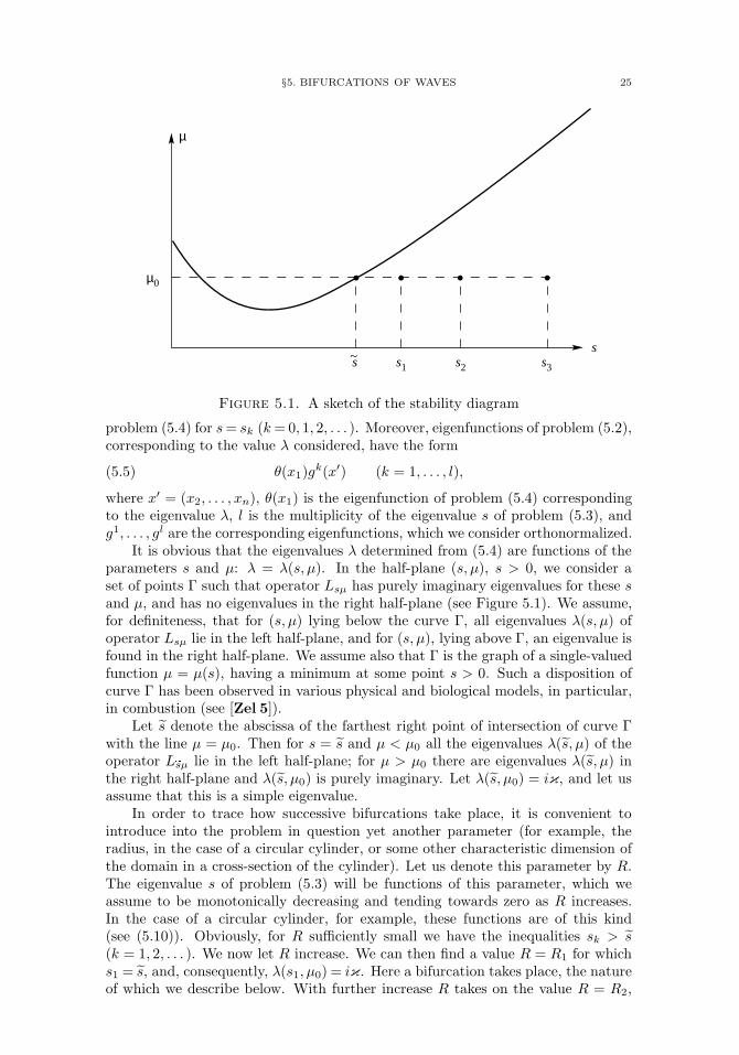
Figure 5.1. A sketch of the stability diagram
problem (5.4) for s= sk (k= 0, 1, 2, . . . ). Moreover, eigenfunctions of problem (5.2),corresponding to the value λ considered, have the form
(5.5) θ(x1)gk(x′) (k = 1, . . . , l),
where x′ = (x2, . . . , xn), θ(x1) is the eigenfunction of problem (5.4) correspondingto the eigenvalue λ, l is the multiplicity of the eigenvalue s of problem (5.3), andg1, . . . , gl are the corresponding eigenfunctions, which we consider orthonormalized.
It is obvious that the eigenvalues λ determined from (5.4) are functions of theparameters s and µ: λ = λ(s, µ). In the half-plane (s, µ), s > 0, we consider aset of points Γ such that operator Lsµ has purely imaginary eigenvalues for these sand µ, and has no eigenvalues in the right half-plane (see Figure 5.1). We assume,for definiteness, that for (s, µ) lying below the curve Γ, all eigenvalues λ(s, µ) ofoperator Lsµ lie in the left half-plane, and for (s, µ), lying above Γ, an eigenvalue isfound in the right half-plane. We assume also that Γ is the graph of a single-valuedfunction µ = µ(s), having a minimum at some point s > 0. Such a disposition ofcurve Γ has been observed in various physical and biological models, in particular,in combustion (see [Zel 5]).
Let s denote the abscissa of the farthest right point of intersection of curve Γwith the line µ = µ0. Then for s = s and µ < µ0 all the eigenvalues λ(s, µ) of theoperator L
esµ lie in the left half-plane; for µ > µ0 there are eigenvalues λ(s, µ) inthe right half-plane and λ(s, µ0) is purely imaginary. Let λ(s, µ0) = iκ, and let usassume that this is a simple eigenvalue.
In order to trace how successive bifurcations take place, it is convenient tointroduce into the problem in question yet another parameter (for example, theradius, in the case of a circular cylinder, or some other characteristic dimension ofthe domain in a cross-section of the cylinder). Let us denote this parameter by R.The eigenvalue s of problem (5.3) will be functions of this parameter, which weassume to be monotonically decreasing and tending towards zero as R increases.In the case of a circular cylinder, for example, these functions are of this kind(see (5.10)). Obviously, for R sufficiently small we have the inequalities sk > s(k = 1, 2, . . . ). We now let R increase. We can then find a value R = R1 for whichs1 = s, and, consequently, λ(s1, µ0) = iκ. Here a bifurcation takes place, the natureof which we describe below. With further increase R takes on the value R = R2,
26 INTRODUCTION. TRAVELING WAVES DESCRIBED BY PARABOLIC SYSTEMS
for which s2 = s, so that λ(s2, µ0) = iκ. The next bifurcation then occurs, and soforth.
Figure 5.1 depicts the case for R sufficiently small.
5.3. A study of bifurcating waves. In place of µ we introduce the parame-ter ε, equal to the norm of the deviation of the sought-for solution u from the planarwave w. We then have the following expansion in powers of the small parameter ε:
(5.6)u = w + εy1 + ε2y2 + · · · , c = c+ ε2c2 + · · · ,µ = µ0 + ε2µ2 + · · · , ω = ω0 + ε2ω2 + · · · ,
coefficients of which can be determined sequentially. Moreover, it may be shownthat y1 is a solution of the linearized problem and has the form
(5.7) y1 =l∑k=1
Re[αkθ(x1)gk(x′) exp(iτ)],
where θ(x1)gk(x′) are the eigenfunctions of problem (5.2) for λ = iκ, µ = µ0, andαk are complex constants,
(5.8)l∑k=1
|αk|2 = 1.
Constants αk are determined from a third step of expansion (5.6) by solvinga system of algebraic equations obtained from conditions for solvability of thenonhomogeneous linearized system: orthogonality of the right-hand sides to thesolutions of the adjoint problem. Such a determination is necessary only in thecase of multiple eigenvalues (l > 1). For l = 1 we can assume that α1 = 1. Weremark that, in spite of the complexity of the systems of equations obtained fordetermining the αk, in all cases in which studies have been made the answer turnedout to be very simple. Thus, for example, for a circular cylinder with l = 2, the αkhave one of the following forms in the generic case:
(5.9)
1) |α1| = 1, α2 = 0,
2) |α2| = 1, α1 = 0,
3) |α1| = |α2| = 2−1/2.
By means of the expansion (5.6) we also prove the existence of bifurcatingwaves, where the word “bifurcating” bears a conditional character. Actually, itfollows from (5.6) that µ > µ0 if µ2 > 0, and that µ < µ0 if µ2 < 0. Both cases arepossible. In the first of these the birth of waves actually takes place during passageof µ through the critical value µ0 (we assume that as µ moves it increases). Suchbifurcations are called supercritical. In the other case the waves in question coexistwith a stable planar wave w and, during passage of µ through a critical value, theydisappear. We call such bifurcations subcritical.
Stability may also be studied by means of expansions with respect to a smallparameter. It turns out that in the case of a simple eigenvalue (l = 1) subcriticalbifurcations are unstable and supercritical bifurcations are stable. In the case ofmultiple eigenvalues (l > 1) unstable supercritical bifurcations are also possible.
We illustrate the above with examples from frequently encountered cases: acircular cylinder; a strip; a cylindrical domain with square cross-section.
§5. BIFURCATIONS OF WAVES 27
Circular cylinder. In this case the eigenvalues s and eigenfunctions g ofproblem (5.3) have the form
(5.10) s = σ2mk/R2, g = Jm(rσmk/R) exp(±imϕ) (m, k = 0, 1, 2, . . . ).
Here Jm is a Bessel function of order m; σmk are the consecutive zeros of itsderivative; R is the radius of the circle; and r and ϕ are polar coordinates.
When m = 0 the eigenvalues are simple and equation (5.7) takes the form
(5.11) y1 = Re[θ(x1) exp(iτ)]J0(rσ0k/R).
For m > 0 the eigenvalues of problem (5.3) are double. As was remarked above,the αk in this case are given by equations (5.9). To begin, we consider the first ofthese equations. Setting α1 = exp(is1), where s1 is a real parameter, we obtain
(5.12) y1 = Re[θ(x1) exp i(±mϕ+ τ + s1)]Jm(rσmk/R),
where we take the + sign for mϕ. For the second of the equations (5.9) the resultis similar: y1 is given by equation (5.12) with the − sign for mϕ.
In the case of the third of equations (5.9) it is convenient to set αj =2−1/2 exp(isj)(j = 1, 2), where sj are arbitrary real constants. Introducing new arbitraryconstants ϕ0 and τ0: s1 = kϕ0 + τ0, s2 = −kϕ0 + τ0, we obtain
(5.13) y1 = Re[θ(x1) exp i(τ + τ0)]Jm(rσmk/R) cosm(ϕ+ ϕ0)
(positive constant factors in y1 have been omitted).Equations (5.11)–(5.13) include all modes of wave propagation present in a
circular cylinder for the bifurcations considered. More precisely, we have indicatedthe leading terms in the expansions in powers of the small parameter ε for all thesemodes. In this way, we see that the leading terms of the expansion are written outexplicitly with respect to the transverse variables, and we can describe the wavesconsidered by these leading terms. This is conveniently done by tracing the motionof an arbitrary characteristic point. As such points we can take the maxima ofa component of vector y1. In combustion this corresponds to what is observedexperimentally: the motion of luminous spots, of which we spoke in §1, namely,points of maximum temperature. Naturally, higher order terms in expansion (5.6)can also contribute, but this does not change the character of the mode considered.This is confirmed by the good agreement of the waves described in this way withexperimental observations.
We shall describe bifurcations in the order in which they arise as the cylinderradiusR increases, in accordance with the description given in the preceding section.This order is determined by the sequence of eigenvalues of problem (5.3), taken inincreasing order. By virtue of (5.10) this is determined by the description of thezeros of the derivatives of the Bessel functions. Figure 5.2 shows graphs of Besselfunctions of orders m = 0, 1, 2, 3 and zeros of their derivatives. For m > 3 positivezeros of the derivatives are found to the right. It is evident from this figure thatthe positive zeros of the derivatives are located in such a sequence,
(5.14) σ11, σ21, σ01, σ31, σ12, . . . .
We consider the equality
(5.15) sj = s (j = 1, 2, . . . ),
where the sj are consecutive positive eigenvalues of problem (5.3), and s is the
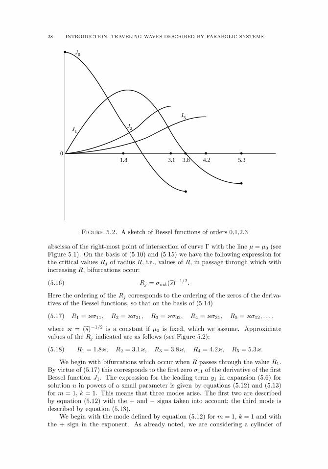
28 INTRODUCTION. TRAVELING WAVES DESCRIBED BY PARABOLIC SYSTEMS
01.8 3.1 3.8 4.2 5.3
J0
J1J2
J3
Figure 5.2. A sketch of Bessel functions of orders 0,1,2,3
abscissa of the right-most point of intersection of curve Γ with the line µ = µ0 (seeFigure 5.1). On the basis of (5.10) and (5.15) we have the following expression forthe critical values Rj of radius R, i.e., values of R, in passage through which withincreasing R, bifurcations occur:
(5.16) Rj = σmk(s)−1/2.
Here the ordering of the Rj corresponds to the ordering of the zeros of the deriva-tives of the Bessel functions, so that on the basis of (5.14)
(5.17) R1 = κσ11, R2 = κσ21, R3 = κσ02, R4 = κσ31, R5 = κσ12, . . . ,
where κ = (s)−1/2 is a constant if µ0 is fixed, which we assume. Approximatevalues of the Rj indicated are as follows (see Figure 5.2):
(5.18) R1 = 1.8κ, R2 = 3.1κ, R3 = 3.8κ, R4 = 4.2κ, R5 = 5.3κ.
We begin with bifurcations which occur when R passes through the value R1.By virtue of (5.17) this corresponds to the first zero σ11 of the derivative of the firstBessel function J1. The expression for the leading term y1 in expansion (5.6) forsolution u in powers of a small parameter is given by equations (5.12) and (5.13)for m = 1, k = 1. This means that three modes arise. The first two are describedby equation (5.12) with the + and − signs taken into account; the third mode isdescribed by equation (5.13).
We begin with the mode defined by equation (5.12) for m = 1, k = 1 and withthe + sign in the exponent. As already noted, we are considering a cylinder of
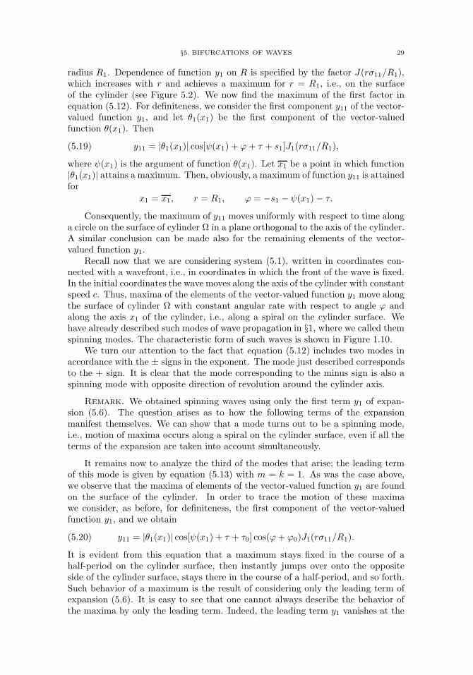
§5. BIFURCATIONS OF WAVES 29
radius R1. Dependence of function y1 on R is specified by the factor J(rσ11/R1),which increases with r and achieves a maximum for r = R1, i.e., on the surfaceof the cylinder (see Figure 5.2). We now find the maximum of the first factor inequation (5.12). For definiteness, we consider the first component y11 of the vector-valued function y1, and let θ1(x1) be the first component of the vector-valuedfunction θ(x1). Then
(5.19) y11 = |θ1(x1)| cos[ψ(x1) + ϕ+ τ + s1]J1(rσ11/R1),
where ψ(x1) is the argument of function θ(x1). Let x1 be a point in which function|θ1(x1)| attains a maximum. Then, obviously, a maximum of function y11 is attainedfor
x1 = x1, r = R1, ϕ = −s1 − ψ(x1)− τ.
Consequently, the maximum of y11 moves uniformly with respect to time alonga circle on the surface of cylinder Ω in a plane orthogonal to the axis of the cylinder.A similar conclusion can be made also for the remaining elements of the vector-valued function y1.
Recall now that we are considering system (5.1), written in coordinates con-nected with a wavefront, i.e., in coordinates in which the front of the wave is fixed.In the initial coordinates the wave moves along the axis of the cylinder with constantspeed c. Thus, maxima of the elements of the vector-valued function y1 move alongthe surface of cylinder Ω with constant angular rate with respect to angle ϕ andalong the axis x1 of the cylinder, i.e., along a spiral on the cylinder surface. Wehave already described such modes of wave propagation in §1, where we called themspinning modes. The characteristic form of such waves is shown in Figure 1.10.
We turn our attention to the fact that equation (5.12) includes two modes inaccordance with the ± signs in the exponent. The mode just described correspondsto the + sign. It is clear that the mode corresponding to the minus sign is also aspinning mode with opposite direction of revolution around the cylinder axis.
Remark. We obtained spinning waves using only the first term y1 of expan-sion (5.6). The question arises as to how the following terms of the expansionmanifest themselves. We can show that a mode turns out to be a spinning mode,i.e., motion of maxima occurs along a spiral on the cylinder surface, even if all theterms of the expansion are taken into account simultaneously.
It remains now to analyze the third of the modes that arise; the leading termof this mode is given by equation (5.13) with m = k = 1. As was the case above,we observe that the maxima of elements of the vector-valued function y1 are foundon the surface of the cylinder. In order to trace the motion of these maximawe consider, as before, for definiteness, the first component of the vector-valuedfunction y1, and we obtain
(5.20) y11 = |θ1(x1)| cos[ψ(x1) + τ + τ0] cos(ϕ+ ϕ0)J1(rσ11/R1).
It is evident from this equation that a maximum stays fixed in the course of ahalf-period on the cylinder surface, then instantly jumps over onto the oppositeside of the cylinder surface, stays there in the course of a half-period, and so forth.Such behavior of a maximum is the result of considering only the leading term ofexpansion (5.6). It is easy to see that one cannot always describe the behavior ofthe maxima by only the leading term. Indeed, the leading term y1 vanishes at the
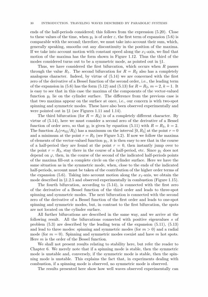
30 INTRODUCTION. TRAVELING WAVES DESCRIBED BY PARABOLIC SYSTEMS
ends of the half-periods considered; this follows from the expression (5.20). Closeto these values of the time, when y1 is of order ε, the first term of expansion (5.6) iscomparable with the second; therefore, we must take into account their sum, which,generally speaking, smooths out any discontinuity in the position of the maxima.If we take into account motion with constant speed along the x1-axis, we find thatmotion of the maxima has the form shown in Figure 1.12. Thus the third of themodes considered turns out to be a symmetric mode, as pointed out in §1.
Thus, we have considered the first bifurcation, which occurs when R passesthrough the value R1. The second bifurcation for R = R2 also has a completelyanalogous character. Indeed, by virtue of (5.14) we are concerned with the firstzero of the derivative of a Bessel function of the second order, i.e., the leading termof the expansion in (5.6) has the form (5.12) and (5.13) for R=R2, m= 2, k = 1. Itis easy to see that in this case the maxima of the components of the vector-valuedfunction y1 lie on the cylinder surface. The difference from the previous case isthat two maxima appear on the surface at once, i.e., our concern is with two-spotspinning and symmetric modes. These have also been observed experimentally andwere pointed out in §1 (see Figures 1.11 and 1.14).
The third bifurcation (for R = R3) is of a completely different character. Byvirtue of (5.14), here we must consider a second zero of the derivative of a Besselfunction of order zero, so that y1 is given by equation (5.11) with R = R3, k = 2.The function J0(rσ02/R3) has a maximum on the interval [0, R3] at the point r = 0and a minimum at the point r = R3 (see Figure 5.2). If now we follow the maximaof elements of the vector-valued function y1, it is then easy to see that in the courseof a half-period they are found at the point r = 0, then instantly jump over tothe point r = R3, stay there in the course of a half-period, etc. Since y1 does notdepend on ϕ, then, in the course of the second of the indicated half-periods pointsof the maxima fill-out a complete circle on the cylinder surface. Here we have thesame situation as in the symmetric mode, when, close to the ends of the indicatedhalf-periods, account must be taken of the contribution of the higher order terms ofthe expansion (5.6). Taking into account motion along the x1-axis, we obtain themode described in §1.2.5 and observed experimentally in combustion (Figure 1.15).
The fourth bifurcation, according to (5.14), is connected with the first zeroof the derivative of a Bessel function of the third order and leads to three-spotspinning and symmetric modes. The next bifurcation is connected with the secondzero of the derivative of a Bessel function of the first order and leads to one-spotspinning and symmetric modes, but, in contrast to the first bifurcation, the spotsare not located on the cylinder surface.
All further bifurcations are described in the same way, and we arrive at thefollowing result. All the bifurcations connected with positive eigenvalues s ofproblem (5.3) are described by the leading term of the expansion (5.11), (5.13)and lead to three modes: spinning and symmetric modes (for m > 0) and a radialmode (for m = 0). Spinning and symmetric modes coexist and have m hot spots.Here m is the order of the Bessel function.
We shall not present results relating to stability here, but refer the reader toChapter 6. We merely note that if a spinning mode is stable, then the symmetricmode is unstable and, conversely, if the symmetric mode is stable, then the spin-ning mode is unstable. This explains the fact that, in experiments dealing withcombustion, if a spinning mode is observed, no symmetric mode is observed.
The results presented here show how well waves observed experimentally can
§5. BIFURCATIONS OF WAVES 31
Figure 5.3. One-spot mode of wave propagation in a strip
be described with the aid of the theory of bifurcations. It should be noted, however,that only waves close to a planar wave can be studied with the aid of this theory.A study of well-developed modes at a distance from a planar wave already requirescomputer calculations. It is, nevertheless, a remarkable fact that both calculationsand physical experiment show that developed modes have the very same characteras nascent modes, i.e., during the birth of modes their fundamental characteristicfeatures are already manifest. These modes persist up to secondary bifurcations.Computer calculations of developed modes for similar problems were carried outin [Bay 5, Ivl 1, 2, Sch 1, 2, Vol 46]. One of the results is the following: aspinning mode appearing during the first bifurcation (R = R1) is maintained up tothe second bifurcation (R=R2), and then two stable modes are present, a one-spotspinning and a two-spot spinning mode.
Strip. In two-dimensional space, the cylinder Ω converts to a strip: −∞< x1 <∞, 0 x2 R, and problem (5.3) has the form
(5.21)d2g
dx22+ sg = 0,
dg
dx2
∣∣∣∣x2=0,x2=R
= 0.
The eigenvalues s are simple, and the first term of expansion (5.6), in accordancewith equation (5.7), has the form
y1 = Re[θ(x1) exp(iτ)] cos(kπx2/R),
where, assuming that s > 0, k takes on the values 1, 2, . . . . Upon studying, aswe did above, the maxima of components of this vector-valued function, we obtainwave propagation modes which, by analogy with combustion, can be called one-spot modes, two-spot modes, etc. The character of the motion of the spots (of themaxima) is shown in Figures 5.3 and 1.9. Figure 5.3 shows a one-spot mode in theform in which it is obtained using the first term y1 of expansion (5.6); Figure 1.9shows a two-spot mode with the contribution of succeeding terms of the expansiontaken into account.
Cylindrical domain with square cross-section (−∞ < x1 <∞, 0 x2, x3 R).Eigenvalues s of problem (5.3) can have different multiplicity. The first term y1 ofexpansion (5.6) has, in accordance with equation (5.7), the form
y1 = Re[θ(x1) exp(iτ) cos(kπx2/R) cos(lπx3/R)],
where k and l are nonnegative integers. Without stopping to give a full descriptionof the possible modes, we cite some examples. When k = l = 1, the mode thatappears represents (Figure 1.16) the simultaneous motion of two hot spots alongopposite edges of the cylinder, with their subsequent transition to two other edges
32 INTRODUCTION. TRAVELING WAVES DESCRIBED BY PARABOLIC SYSTEMS
of the cylinder, etc. For k = l = 2 the mode obtained is shown in Figure 1.17 andis a mode observed in combustion. A study has shown, in the case of eigenvaluess of problem (5.3) of multiplicity two, that a simultaneous bifurcation of modesof two types is possible (analogous to the appearance of spinning and symmetricmodes in a circular cylinder), and, under certain conditions, modes of three types.In the case of multiple eigenvalues (as is well known, problem (5.3) in a square haseigenvalues of arbitrary large multiplicity) the problem of explaining the number ofmodes emerging and their form reduces to the solution of some algebraic equations.
Nonlinear stability analysis of specific combustion models is discussed in thesupplement to Part III. We note finally that some problems of bifurcations of wavesare studied in [Bar 1, 2, Gils 1, Kop 4, Nis 2].
§6. Traveling waves in physics, chemistry, and biology
Studies of wave solutions of parabolic equations evolved, to a significant degree,under the influence of problems of physics, chemistry, and biology. A majorrole here was played by Kolmogorov, Petrovskiı, and Piskunov [Kolm 1] and byFisher [Fis 1] on the propagation of dominant genes; by Zel′dovich and Frank-Kamenetskiı [Zel 2, 5, Fran 1] on combustion theory; and by Semenov on coldflames [Vor 1, Sem 1].
Many physical, chemical, and biological phenomena which were observed ex-perimentally and can be modeled by traveling wave solutions of parabolic systemsare discussed in [Vas 2]. There are also many other works devoted to a descriptionand investigation of this kind of models (see [Aut 1, Baren 1, Buc 7, Dik 1,Dyn 1, Fife 1, 2, Gray 2, Grin 3, Gus 1, Had 1, Iva 1, Korob 1, Kuz 1,Lan 1, Luk 1, 2, Mas 1, Mur 1, Non 1, 2, Nov 2, Pro 1, Rab 1, Rom 1, 2,Sco 1, 2, Sem 2–5, Svi 1, 2, Vol 47, Zel 5–11, Zha 1, Zve 1]).
Most of the mathematical works are devoted to traveling waves describedby the equations of chemical kinetics (some biological models lead to the samemathematical models), combustion, and propagation of nerve impulse.
It was mentioned above that propagation of nerve impulse can be described bythe Hodgkin-Huxley equations or by simpler Fitz-Hugh-Nagumo equations. Thelatter have form
∂u1∂t
=∂2u1∂x2
+ F (u1)− u2,
∂u2∂t
= bu1,
where b is a constant, F is a given function.There are many works devoted to the problem of existence of impulses, systems
of impulses, periodic waves, and to the problem of their stability and to otherproblems (see [Bel 2, Car 1–3, Cas 1, Eva 1–6, Fer 1, 2, Has 1–3, Kla 3,Liu 1, 2, McK 2, Rau 1, Rin 1–3, Schon, Tal 1, Troy 1, Yan 1, 2] and thereferences presented in §3 and in §5 of Chapter 3).
We discuss now in more detail the models of chemical kinetics and combustion.Part III of the book is devoted to the investigation of these models.
We consider a chemical reaction in which substances taking part (and beinggenerated) are denoted by A1, . . . , Am and which is described by n elementary
§6. TRAVELING WAVES IN PHYSICS, CHEMISTRY, AND BIOLOGY 33
reactions (stages)
(6.1)m∑j=1
αijAj −→m∑j=1
βijAj (i = 1, . . . , n),
the nonnegative integers αij (or βij), which indicate how many molecules of reagentAj take part (or are formed) in the reaction, are called stoichiometric coefficients.
The rate of the ith reaction, i.e., the rate of transformation of the initialsubstances into the reaction products, can be written in the form
(6.2) Φi = Aαi11 × · · · ×Aαim
m ki(T ),
where T is the temperature, ki(T ) are the thermal coefficients of the reaction rate,and the Ai are the concentrations of substances Ai. Expression (6.2) is writtenunder the assumption that the law of mass action is satisfied (see, e.g., [Den 1]).
If we assume that the concentrations of all the substances are distributed inspace uniformly, then their change with time may be described by the kinetic(nondistributed) system of equations
(6.3)dA
dt= ΓΦ,
where A = (A1, . . . , Am), Φ = (Φ1, . . . ,Φn), γij = βij − αij , and
Γ =
γ11 · · · γn1· · · · · · · · ·γ1m · · · γnm
.But if the concentrations are distributed nonuniformly in space, and the chemi-cal reaction is accompanied by diffusion of components, then the distribution ofconcentrations in time and space is described by the parabolic system of equations
(6.4)∂A
∂t= d∆A+ ΓΦ,
where d is the coefficient of diffusion, which here, for simplicity, we assume to bethe same for all substances and constant; ∆ is the Laplace operator.
A chemical reaction may be accompanied by liberation or absorption of heat.In this case system (6.4) must be supplemented by the heat conduction equation
(6.5)∂T
∂t= κ∆T +
n∑i=1
qiΦi,
where qi is the adiabatic heating due to the ith reaction, and κ is the thermaldiffusivity coefficient. These quantities are assumed to be constants.
We have presented here a thermal diffusion model of combustion in which noaccount is taken of the influence of hydrodynamic factors on the propagation of awave of combustion. Without going into detail on the question of its applicability,we point out that in a number of cases the influence of hydrodynamics can beneglected [Zel 5].
We now present some of the simplest and most frequently encountered specialcases of system (6.4), (6.5), limiting ourselves here to the case of one spatial variable(for bibliographical commentaries see the supplement to Part III).
34 INTRODUCTION. TRAVELING WAVES DESCRIBED BY PARABOLIC SYSTEMS
A single-stage reaction of the nth order
nA −→ B,
accompanied by heat liberation, may be described by the system of equations
(6.6)
∂T
∂t= κ
∂2T
∂x2+ qk(T )An,
∂A
∂t= d
∂2A
∂x2− k(T )An.
In moving coordinates connected with a wave the stationary system has the form
(6.7)dA′′ − cA′ − k(T )An = 0,
κT ′′ − cT ′ + qk(T )An = 0,
where c is the wave speed. Conditions at infinity are given by
T (−∞) = T0, A(−∞) = 1,
T (+∞) = Tb, A(+∞) = 0.
Here T0 is the initial temperature of the mixture and Tb is the burning temperature,which is obtained from a first integral of the problem; Tb = T0 + q.
This model is, apparently, the most widely used in the theory of waves ofcombustion and is a model on which studies of many features of combustionprocesses have been made. Above all, we note that the function k(T ) is stronglynonlinear and increases rapidly with an increase in temperature. As a rule theArrhenius temperature dependence of the reaction rate,
k(T ) = k0 exp(−E/RT ),
is considered. Here E is the activation energy of the chemical reaction, R is theuniversal gas constant, and k0 is a pre-exponential factor. For large values ofactivation energy, which are characteristic of combustion processes, the chemicalreaction rate for low temperatures close to T0 is many orders less than the reactionrate for high temperatures close to Tb. We can therefore set k(T ) ≡ 0 for T T∗,where T∗ : T0 < T∗ < Tb, the so-called cutting-off temperature of the source. Thisguarantees equality to zero of the reaction rate for x = −∞, and, consequently,fulfillment of the necessary condition for existence of a wave solution. The approachindicated expresses the fact that a stationary combustion wave is an intermediateasymptotic behavior [Baren 4, 5] of a nonstationary wave, i.e., it exists up to thosetimes of a process when the initial conditions are already forgotten and the reactionin the cold mixture is still negligibly small. The approach associated with cutting-off the source requires some justification showing that all the characteristics of acombustion wave depend weakly on a cutting-off temperature selected over a widerange. These questions are discussed in Chapter 10 on the basis of the minimaxrepresentation of the speed described above.
A strong dependence of the reaction rate on the temperature means that thechemical reaction occurs mainly in a narrow temperature interval for temperaturesclose to the combustion temperature, since for lower temperatures the combustionrate is relatively small. This makes it possible to apply an approximate approach,in which it is assumed that the reaction occurs only at a certain point, at whichsolutions of linear equations (6.7) (without a source) obtained to the left and
§6. TRAVELING WAVES IN PHYSICS, CHEMISTRY, AND BIOLOGY 35
to the right of the reaction zone must be matched, according to specific rules.This approach allows approximate determination of the speed of a combustionwave [Zel 1, 2] and of the stability boundary of a stationary wave with respect tosmall perturbations [Baren 3]. Results obtained by the method described abovehave been compared many times with the results of numerical calculations andasymptotic approaches and, as a rule, they turn out to be fairly precise (see thesupplement to Part III).
The nature of the loss of stability of a combustion wave depends on the Lewisnumber Le = κ/d. If Le > 1, then the loss of stability with a change in theparameters of a system occurs in an oscillatory manner: for an operator linearizedon a wave a pair of complex conjugate eigenvalues passes from the left half-planeof the complex plane into the right half-plane across the imaginary axis. In thiscase a Hopf bifurcation occurs (see §5) and, instead of the propagation of a planarcombustion wave with constant speed, there may be established either an auto-oscillation (in the one-dimensional case) or spinning modes or other spatial modes(in the multi-dimensional case) described in §1.
If Le< 1, an eigenvalue of the linearized operator passes into the right half-planethrough zero, and, in the multi-dimensional case, a stationary mode is establishedwith a curved reaction front. When we further move into the domain of instability,the indicated modes can, in turn, lose their stability, new modes then appear, andso forth, up to the appearance of chaotic regimes.
For a fixed value of the Lewis number the stability of a wave is determinedby the value of the dimensionless parameter Z = qE/(2RT 2
b ): for Z < Zcr(Le)the stationary wave is stable; for Z > Zcr(Le) it is unstable. The closer the Lewisnumber approaches 1, the wider becomes the domain of stability: Zcr(Le)→∞ asLe→ 1.
When Le = 1, values of the temperature and concentration in a stationarycombustion wave are related linearly; this allows us to reduce problem (6.6) to ascalar equation. Stability of a wave in this case was first proved in [Baren 2], andthe approach to a wave in this case was discussed in [Kan 3] and [Kolm 1]. In thesequel these questions are discussed in a whole series of papers (see Part I).
Existence of waves for system (6.6) was established in [Kan 4]. It was shownthere that for d < κ the wave is unique. In [Bac 1] for d > κ it was shown, fora specially selected model (somewhat different from (6.6)), that the wave can benonunique.
The next step, using a more complicated model of combustion, is the consid-eration, after (6.6), of the simplest problems of stage combustion. The problemsmost investigated are waves of combustion in which we have:
successive reactions A −→ B, B −→ C;
independent reactions A −→ B, C −→ D;
competing reactions A −→ B, A −→ C.
Other model schemes have also been considered. Various combustion modes havebeen studied, including their stability; it was shown, in particular, that in the caseof competing reactions the combustion wave can be nonunique (see the supplementto Part III).
In Chapter 9 combustion waves are studied for a sufficiently general kinetics ofa chemical reaction. The existence of waves is proved under specific assumptions on
36 INTRODUCTION. TRAVELING WAVES DESCRIBED BY PARABOLIC SYSTEMS
the reaction scheme (6.1). In a number of cases the system of equations (6.4), (6.5)is reduced to a monotone system, making it possible to prove stability of waves andto obtain a minimax representation of the speed.
In the study of combustion waves it may be assumed, as has already beenstated, that the reaction rate at low temperatures is very small, lacking which acombustion wave cannot exist. A somewhat different situation occurs for chainflames, a study of which was initiated by Semenov [Vor 1, Sem 1]. The simplestmodel in which a cold (chain) flame can be realized has the form
(6.8)
d1A′′ − cA′ − kABn = 0,
d2B′′ − cB′ + kABn = 0,
x→ −∞ : A = 1, B = 0,x→ +∞ : A = 0, B = 1.
This system of equations describes the propagation of a wave of a chemical trans-formation for an auto-catalytic reaction
A+ nB −→ (n+ 1)B.
If d1 = d2, then the concentrations are connected by means of the relation A+B =1and the system of equations (6.8) may be reduced to a single equation for whichquestions of existence, stability, and the determination of wave speed have been wellstudied (see Chapter 1). We note that for n = 1 this equation becomes the KPPequation. This abbreviation is often used to denote the work [Kolm 1] and thetype of nonlinearity considered there. The case d1 = d2 was considered in [Bil 1–3].
There are papers in which other models of chain flames are discussed. A seriesof models of such processes is examined in Chapter 8. This also discusses one of themodels of the Belousov-Zhabotinsky reaction, which has been the subject of manypapers.
Mathematical models close to those considered, to which methods developedin this book can be applied, also arise in heterogeneous catalysis (see Chapter 8)in the study of combustion processes in a stream [Kha 9, Mer 9, Vol 17, Zai 1]and also in several other areas of chemical kinetics and combustion [Ald 15, 17,Bow 1, Ter 6]. We remark also that a number of models in biology and ecologymay be described by systems of equations of chemical kinetics type.
Part I
Stationary Waves
CHAPTER 1
Scalar Equation
§1. Introduction
In this chapter we consider waves described by the scalar parabolic equation
(1.1)∂u
∂t=∂2u
∂x2+ F (u).
Function u(x, t) is defined for −∞ < x < +∞, t 0; the initial condition
(1.2) u(x, 0) = f(x)
is assumed to be bounded and piecewise-continuous with a finite number of pointsof discontinuity; F (u) is a continuously differentiable function.
As already indicated, by a solution of traveling wave type (or, for simplicity, awave) we mean a solution of equation (1.1) of the form
u(x, t) = w(x − ct),
where c is a constant called the speed of the wave. We assume that w(x) is boundedon the whole axis and twice continuously differentiable. Obviously, function w(x)satisfies the equation
(1.3) w′′ + cw′ + F (w) = 0,
or the system of two first order equations
(1.4) w′ = p, p′ = −cp− F (w).
Along with the function w(x), the function w(x + h) is also a solution ofequation (1.3) for arbitrary h, −∞ < h < +∞. Therefore, each wave generatesa one-parameter family of solutions of equation (1.3), which are obtained fromone another by a translation in x. Later on, whenever necessary, we impose anadditional condition, allowing us to single-out one of the solutions of this family.
Waves described by a scalar equation can be monotone in x, periodic in x, andnonmonotone, but having the limits
(1.5) limx→±∞
w(x) = w±.
In those cases where we need to indicate values of limits of function w(x) as x→±∞,we call such waves [w+, w−]-waves (w+ < w−). In the main, here, we consider
39
40 1. SCALAR EQUATION
monotone waves, since they, in contrast to nonmonotone waves, are stable (see §5).In §3 we shall show that if the limits (1.5) exist and the inequality
w+ w(x) w−, −∞ < x < +∞,
holds, the wave is then monotone, the derivatives w′(x) and w′′(x) tend to zero asx→ ±∞, and the values w = w± are zeros of function F (w),
(1.6) F (w+) = F (w−) = 0
(equation (1.6) follows from (1.5) even for nonmonotone waves). Therefore, for theexistence of monotone waves it is obviously necessary that there exist at least twozeros of function F (w). (Formally, the function w(x) ≡ w± is also a wave; however,such degenerate waves are not considered here.)
The properties of function F (w) determine the existence of waves, their number,and their stability. Therefore, in what follows, our study of waves is made takinginto account the type of the nonlinear source. We recall here the classification ofsources given in the Introduction. A function F (w), given on the interval [a, b](a < b) and vanishing at its endpoints (F (a) = F (b) = 0), is a source of Type A onthis interval if points a and b are stable stationary points of the equation
(1.7)du
dt= F (u),
with respect to this interval; it is a source of Type B if one of the stationary pointsis stable (see Figure 1.1a) and the other unstable; finally, it is a Type C source ifboth points are unstable.
Other names appearing in the literature will be also used for these types ofsources. A source of Type A corresponds to the bistable case, Type B to themonostable case, and Type C to the unstable case.
It is obvious that point a is stable (with respect to interval [a, b]) if functionF (w) is negative in some right half-neighborhood of this point or vanishes on somesequence wn, wn > a, converging to a as n→∞. In the first instance we use thenotation F (w) ∈ r−(a); in the second instance we use the notation F (w) ∈ r0(a).If function F (w) is positive in some right half-neighborhood of point a, then thisstationary point is unstable and, in this case, we use the notation F (w) ∈ r+(a).We shall use the notation l−(b), l0(b), and l+(b) to indicate the behavior of functionF (w) in a left-neighborhood of point b.
To the solution w(x) of equation (1.3), having the limits (1.5) at infinity, therecorresponds a trajectory (w(x), p(x)) of the system of equations (1.4), joining thesingular points (w−, 0) and (w+, 0) of this system. It is clear that existence andproperties of such trajectories can depend on the type of singular points. It isreadily seen that the eigenvalues of the system, linearized in a neighborhood of asingular point, are calculated as the roots of a quadratic equation,
λ1,2 = −c/2± (c2/4− α)1/2,
where α is the value of the derivative of function F (w) at the corresponding point;for example, α = F ′(w+) for the singular point (w+, 0). Therefore, for α < 0 thesingular point is a saddle point; for α > 0 and c2/4 α it is a node. Moreover,in case c > 0, the node is stable; for c < 0, it is unstable. We note, in the casec2/4 = α, that the eigenvalues take on identical values and that, in some cases, thisproves to be important. In case c2/4 < α, the eigenvalues are complex, and the
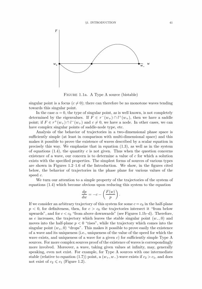
§1. INTRODUCTION 41
F
w+ w−w
Figure 1.1a. A Type A source (bistable)
singular point is a focus (c = 0); there can therefore be no monotone waves tendingtowards this singular point.
In the case α= 0, the type of singular point, as is well known, is not completelydetermined by the eigenvalues. If F ∈ r−(w+) ∩ l+(w+), then we have a saddlepoint; if F ∈ r+(w+) ∩ l−(w+) and c = 0, we have a node. In other cases, we canhave complex singular points of saddle-node type, etc.
Analysis of the behavior of trajectories in a two-dimensional phase space issufficiently simple (at least in comparison with multi-dimensional space) and thismakes it possible to prove the existence of waves described by a scalar equation inprecisely this way. We emphasize that in equation (1.3), as well as in the systemof equations (1.4), the quantity c is not given. Thus when the question concernsexistence of a wave, our concern is to determine a value of c for which a solutionexists with the specified properties. The simplest forms of sources of various typesare shown in Figures 1.2–1.6 of the Introduction. We show, in the figures citedbelow, the behavior of trajectories in the phase plane for various values of thespeed c.
We turn our attention to a simple property of the trajectories of the system ofequations (1.4) which become obvious upon reducing this system to the equation
dp
dw= −c−
(F (w)p
).
If we consider an arbitrary trajectory of this system for some c= c0 in the half-planep < 0, for definiteness, then, for c > c0 the trajectories intersect it “from belowupwards”, and for c < c0 “from above downwards” (see Figures 1.1b–d). Therefore,as c increases, the trajectory which leaves the stable singular point (w−, 0) andmoves into the half-plane p < 0 “rises”, while the trajectory which comes into thesingular point (w+, 0) “drops”. This makes it possible to prove easily the existenceof a wave and its uniqueness (i.e., uniqueness of the value of the speed for which thewave exists, and uniqueness of a wave for a given c) for sufficiently simple Type Asources. For more complex sources proof of the existence of waves is correspondinglymore involved. Moreover, a wave, taking given values at infinity, may, generallyspeaking, even not exist. For example, for Type A sources with one intermediatestable (relative to equation (1.7)) point, a (w+, w−)-wave exists if c2 > c1, and doesnot exist of c2 c1 (Figure 1.2).
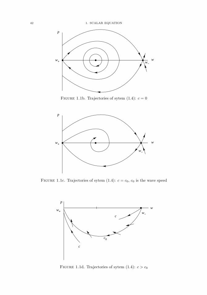
42 1. SCALAR EQUATION
p
w+ w−w
Figure 1.1b. Trajectories of sytem (1.4): c = 0
p
w+
w−
w
Figure 1.1c. Trajectories of sytem (1.4): c = c0, c0 is the wave speed
p
w+ w−
w
c
c
c0
Figure 1.1d. Trajectories of sytem (1.4): c > c0
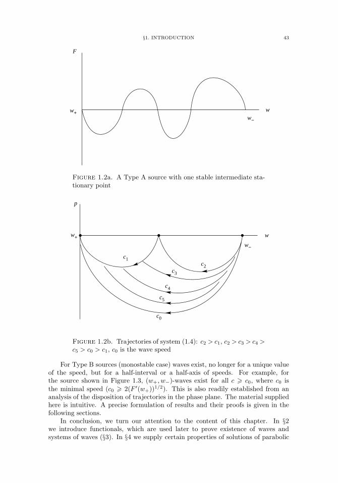
§1. INTRODUCTION 43
w+w−
F
w
Figure 1.2a. A Type A source with one stable intermediate sta-tionary point
p
w+
w−
w
c1c2
c3
c4
c5
c0
Figure 1.2b. Trajectories of system (1.4): c2 > c1, c2 > c3 > c4 >c5 > c0 > c1, c0 is the wave speed
For Type B sources (monostable case) waves exist, no longer for a unique valueof the speed, but for a half-interval or a half-axis of speeds. For example, forthe source shown in Figure 1.3, (w+, w−)-waves exist for all c c0, where c0 isthe minimal speed (c0 2(F ′(w+))1/2). This is also readily established from ananalysis of the disposition of trajectories in the phase plane. The material suppliedhere is intuitive. A precise formulation of results and their proofs is given in thefollowing sections.
In conclusion, we turn our attention to the content of this chapter. In §2we introduce functionals, which are used later to prove existence of waves andsystems of waves (§3). In §4 we supply certain properties of solutions of parabolic
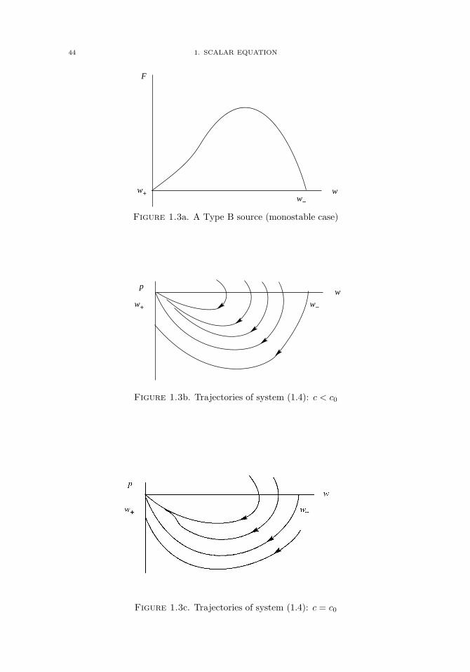
44 1. SCALAR EQUATION
F
w+w−
w
Figure 1.3a. A Type B source (monostable case)
p
w+ w−
w
Figure 1.3b. Trajectories of system (1.4): c < c0
Figure 1.3c. Trajectories of system (1.4): c = c0
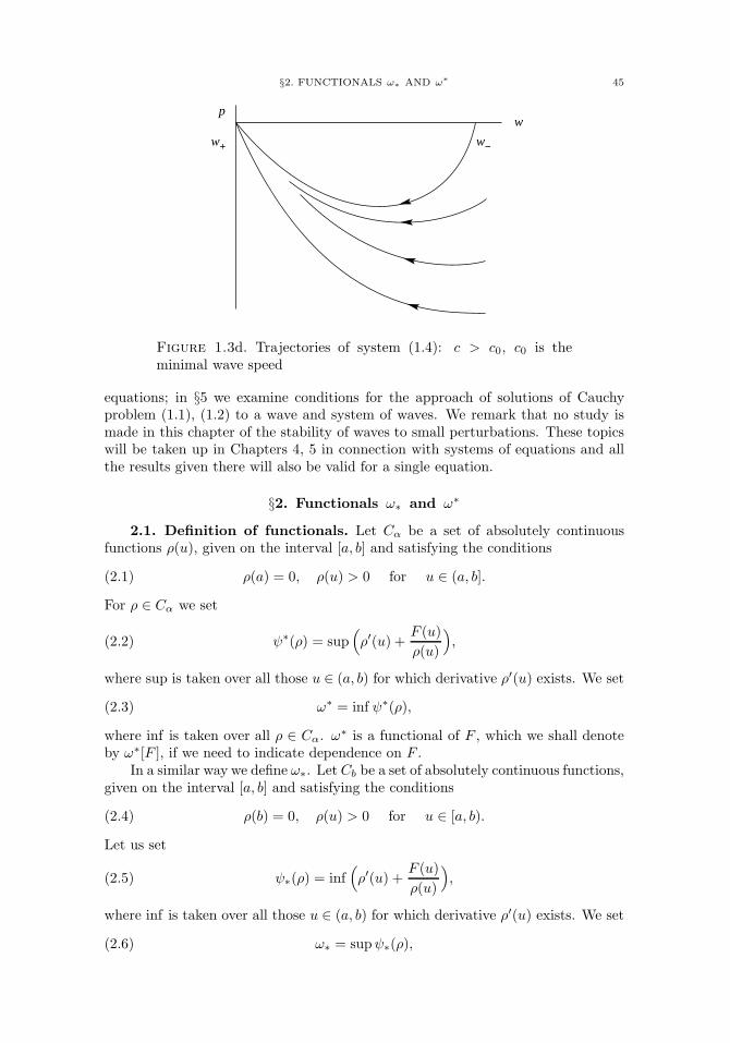
§2. FUNCTIONALS ω∗ AND ω∗ 45
p
w+ w−
w
Figure 1.3d. Trajectories of system (1.4): c > c0, c0 is theminimal wave speed
equations; in §5 we examine conditions for the approach of solutions of Cauchyproblem (1.1), (1.2) to a wave and system of waves. We remark that no study ismade in this chapter of the stability of waves to small perturbations. These topicswill be taken up in Chapters 4, 5 in connection with systems of equations and allthe results given there will also be valid for a single equation.
§2. Functionals ω∗ and ω∗
2.1. Definition of functionals. Let Cα be a set of absolutely continuousfunctions ρ(u), given on the interval [a, b] and satisfying the conditions
(2.1) ρ(a) = 0, ρ(u) > 0 for u ∈ (a, b].
For ρ ∈ Cα we set
(2.2) ψ∗(ρ) = sup(ρ′(u) +
F (u)ρ(u)
),
where sup is taken over all those u ∈ (a, b) for which derivative ρ′(u) exists. We set
(2.3) ω∗ = inf ψ∗(ρ),
where inf is taken over all ρ ∈ Cα. ω∗ is a functional of F , which we shall denoteby ω∗[F ], if we need to indicate dependence on F .
In a similar way we define ω∗. Let Cb be a set of absolutely continuous functions,given on the interval [a, b] and satisfying the conditions
(2.4) ρ(b) = 0, ρ(u) > 0 for u ∈ [a, b).
Let us set
(2.5) ψ∗(ρ) = inf(ρ′(u) +
F (u)ρ(u)
),
where inf is taken over all those u ∈ (a, b) for which derivative ρ′(u) exists. We set
(2.6) ω∗ = supψ∗(ρ),
46 1. SCALAR EQUATION
where sup is taken over all ρ ∈ Cb.
2.2. Connection with solutions of the equation p′ + F/p + c = 0.Consider the equation
(2.7) p′(u) +F (u)p(u)
+ c = 0.
As usual, we denote by C[a, b] and C1(a, b) the sets of functions continuous on [a, b]and having continuous derivatives on (a, b), respectively.
Theorem 2.1. In order for there to exist a solution p(u) of equation (2.7) onthe interval (a, b), satisfying the conditions
(2.8)p ∈ C1(a, b) ∩ C[a, b], p(a) = 0,
p(u) < 0 for u ∈ (a, b],
it is necessary that the inequality
(2.9) c ω∗
be satisfied and sufficient that the inequality
(2.10) c > ω∗
be satisfied.
Proof. Assume that a solution p of problem (2.7), (2.8) exists. Then
ρ = −p ∈ Cα.
From (2.7) we have c = ψ∗(ρ), from whence (2.9) follows. Next, assume thatinequality (2.10) is satisfied. Then there exists a function ρ ∈ Cα such that
ψ∗(ρ) < c.
Consider now a solution pν(u) of equation (2.7) with initial condition pν(α) = −ν,where ν is a sufficiently small positive number. We show that
(2.11) pν(u) < p(u) for u ∈ [a, b],
where p(u) = −ρ(u). Assume the contrary to be true. Then there exists a numberu0 ∈ (a, b] such that
(2.12) pν(u0) = p(u0), pν(u) < p(u) for u ∈ [a, u0).
We now select ε satisfying the inequalities
(2.13) 0 < ε < c− ψ∗(ρ),
and a number u1 ∈ (a, u0), such that
(2.14)1
u0 − u1
∫ u0
u1
[F (u)p(u)
− F (u)pν(u)
]du < ε.
Since pν(u) is a solution of equation (2.7), then
(2.15) pν(u0)− pν(u1) +∫ u0
u1
F (u)pν(u)
du = −c(u0 − u1).
§2. FUNCTIONALS ω∗ AND ω∗ 47
From (2.2) we have
−p′(u)− (F (u)/p(u)) ψ∗(ρ)
almost everywhere on (a, b), from whence we have
p(u0)− p(u1) +∫ u0
u1
(F (u)/p(u)) du −ψ∗(ρ)(u0 − u1).
Subtracting (2.15) from this inequality and taking (2.13) and (2.14) into ac-count, we obtain pν(u1)>p(u1), which contradicts (2.12). Thus we have establishedinequality (2.11).
We now pass to the limit as ν → 0. We obtain the solution p0(u) of equa-tion (2.7), satisfying conditions p0(a) = 0, p0(u) p(u) for u ∈ [a, b]. Thereforep0(u) satisfies conditions (2.8). This completes the proof of the theorem.
Theorem 2.2. In order that there exist a solution p(u) of equation (2.7) onthe interval (a, b), satisfying the conditions
(2.16) p ∈ C1(a, b) ∩ C[a, b], p(b) = 0, p(u) < 0 for u ∈ [a, b),
it is necessary that the inequality
(2.17) c ω∗
be satisfied and sufficient that the inequality
c < ω∗
be satisfied.
The proof of this theorem is similar to the proof of Theorem 2.1.
Corollary. Problem (2.7), (2.8) (problem (2.7), (2.16)) is solvable for at leastone c if and only if ω∗ < ∞ (ω∗ > −∞). Upon satisfaction of this condition,ω∗ = inf c (ω∗ = sup c), where inf (sup) is taken over the set of all c for which thisproblem is solvable.
The proof is obvious.
2.3. Estimates of functionals. Here we present simplest estimates of thefunctionals ω∗ and ω∗, which we shall need later on. We first prove the inequality
(2.18) ω∗ ω∗.
Assume the contrary to be true. Then there exists a number c such that
ω∗ < c < ω∗.
On the basis of Theorems 2.1 and 2.2 there exist solutions of problems (2.7), (2.8)and (2.7), (2.16). These solutions obviously take on equal values for some u ∈ (a, b),which contradicts uniqueness of a solution of the Cauchy problem for equation (2.7).
48 1. SCALAR EQUATION
We introduce the notation
(2.19) γ∗ = supu∈(a,b)
F (u)u− a , γ∗ = inf
u∈(a,b)
F (u)b − u.
Theorem 2.3. We have the following relations :
ω∗ = ω∗ = −∞ if γ∗ < 0,(2.20)
ω∗ = ω∗ =∞ if γ∗ > 0,(2.21)
−2| − γ∗|1/2 ω∗ ω∗ 2|γ∗|1/2 if γ∗ 0, γ∗ 0.(2.22)
Proof. All the inequalities may be proved in the same way, using the functionρ = k(u − a) (k > 0) for estimates of the functional ω∗, and using the functionρ = k(b − u) (k > 0) for estimates of the functional ω∗. We give, for example, theproof of the right-hand inequality in (2.22). For ρ = k(u− a) the functional ψ∗(ρ)(see (2.2)) takes the form
ψ∗(ρ) = k + (γ∗/k).
For γ∗ 0, taking inf over k, we obtain 2(γ∗)1/2. The last inequality in (2.22)follows from this.
Theorem 2.4. Let F (u) ∈ C1[a, b]. Then
(2.23) ω∗ = ω∗ =∞,
if F (b) = 0, F (u) > 0 for u ∈ [a, b), and
(2.24) ω∗ = ω∗ = −∞
if F (a) = 0, F (u) < 0 for u ∈ (a, b].
Proof. We prove equality (2.23). Set ρ(u) = kF (u) (k > 0). We haveψ∗(ρ) = k−1 − σk, where −σ = inf F ′(u) for u ∈ (a, b). It follows from this thatω∗ k−1 − σk → ∞ for k → 0. It remains to make use of inequality (2.18).Equalities (2.24) are proved in the same way.
As mentioned above, we shall write ω∗[F ] and ω∗[F ] for indicating the depen-dence of ω∗ and ω∗ on F .
Theorem 2.5. If F1(u) F2(u), then
(2.25) ω∗[F1] ω∗[F2], ω∗[F1] ω∗[F2].
If F (u) ≡ 0, then
(2.26) ω∗[F ] = ω∗[F ] = 0.
Proof. Inequality (2.25) follows directly from the definition of ω∗ and ω∗;relations (2.26) follow from (2.22). This completes the proof of the theorem.
§2. FUNCTIONALS ω∗ AND ω∗ 49
From (2.25) and (2.26) we obviously have:
ω∗[F ] 0, ω∗[F ] 0 if F (u) 0;(2.27)
ω∗[F ] 0, ω∗[F ] 0 if F (u) 0.(2.28)
Theorem 2.6. We have the inequalities
ω∗[F ] 0 if∫ b
u
F (s) ds 0,(2.29)
ω∗[F ] 0 if∫ u
a
F (s) ds 0,(2.30)
for all u ∈ [a, b].
Proof. To prove inequality (2.29) we set, for arbitrary ε > 0,
ρε(u) =[2∫ b
u
F (s) ds+ ε2(b− u)2]1/2
.
Then ψ∗(ρε) −ε, and inequality (2.29) follows. Inequality (2.30) is proved in asimilar way. This completes the proof of the theorem.
Theorem 2.7. If F ∈ l+(b) and a solution of problem (2.7), (2.16) exists, thenω∗[F ] > c.
If F ∈ r−(α) and a solution of problem (2.7), (2.8) exists, then ω∗[F ] < c.
Proof. We prove the first assertion. The second is proved similarly.On the basis of Theorem 2.2 it is sufficient to show that no solution of prob-
lem (2.7), (2.16) exists for c= ω∗. Assume the contrary: there does exist a solution.Denote it by p∗(u). Let u1< b be such that F (u)> 0 for u∈ [u1, b). By Theorem 2.4,applied to the interval [u1, b], and also Theorem 2.2, we conclude that, for arbitraryfinite c, there exists a solution p(u) of equation (2.7), satisfying conditions p(b) = 0,p(u) < 0 for u ∈ [u1, b). Let c > ω∗ and sufficiently close to ω∗. Then, taking intoaccount the behavior in a neighborhood of the singular point u = b, p = 0 (seeTheorem 3.4), we readily see that p(u) is sufficiently close to p∗(u) on the interval[a, b], and therefore satisfies conditions (2.16). But this contradicts Theorem 2.2.This completes the proof of the theorem.
Corollary. If F ∈ l+(b) and∫ b
u
F (s) ds > 0 for all u ∈ [a, b),
then ω∗[F ] > 0.If F ∈ r−(a) and ∫ u
a
F (s) ds < 0 for all u ∈ (a, b],
then ω∗[F ] < 0.
Proof. The function
p(u) = −[2∫ bu
F (s) ds]1/2
is a solution of problem (2.7), (2.16) with c = 0. The first of the assertions
50 1. SCALAR EQUATION
follows from this. The second is proved similarly. This completes the proof ofthe corollary.
2.4. Dependence on endpoints of the interval. We have defined function-als ω∗ and ω∗ on the interval [a, b]. Let us consider these functionals as functionsof a and b, denoting them by ω∗(a, b) and ω∗(a, b) to indicate dependence on theends of the interval.
Theorem 2.8. Functionals ω∗(a, u) and ω∗(u, b) are nondecreasing functionsof u for u ∈ (a, b] and u ∈ [a, b), respectively.
Proof. Consider the functional ω∗(u, b). The proof proceeds accordingly forω∗(a, u). Let u1 < u2, u1, u2 ∈ [a, b). We need to show that
(2.31) ω∗(u1, b) ω∗(u2, b).
We denote by ψ1∗(ρ) and ψ2∗(ρ) functionals, defined on intervals [u1, b] and [u2, b],just as was done in §2.1 (see (2.5)) for the interval [a, b]. By definition, for arbitraryε > 0 there exists a function ρ ∈ Cb, given on the interval [u1, b], such that
(2.32) ψ1∗(ρ) > ω∗(u1, b)− ε.
Taking the restriction of ρ on the interval [u2, b], we obtain
(2.33) ψ2∗(ρ) ψ1∗(ρ).
From this and from (2.31) and (2.32) we have
ω∗(u2, b) ψ2∗(ρ) ω∗(u1, b)− ε,
from whence, in view of the arbitrariness of ε, (2.31) follows. This completes theproof of the theorem.
Corollary. If F (u) > 0 for a u1 < u < u2 < b, then
(2.34) ω∗(u, b) = ω∗(u2, b) for u1 < u u2.
Proof. Assume that ω∗(u2, b) is finite. By virtue of monotonicity, we have
(2.35) ω∗(u, b) ω∗(u2, b)
for u u2. Let c be an arbitrary number:
(2.36) c < ω∗(u2, b).
Then, based on Theorem 2.2, there exists a solution p(u) of equation (2.7) satisfyingthe conditions
p(b) = 0, p(u) < 0 for u2 u < b.
We extend this solution for u < u2. Then p(u) < 0 for u1 < u < u2, by virtueof equation (2.7), in view of the positivity of F (u). Applying Theorem 2.2 to theinterval [u, b], we obtain c ω∗(u, b). Since c is an arbitrary number satisfyinginequality (2.36), it follows that ω∗(u2, b) ω∗(u, b). Relation (2.34) then followsfrom this and from (2.35). For infinite values of ω∗(u2, b) the proof is equally simple.This completes the proof of the theorem.
There is an analogous corollary for ω∗.
§3. WAVES AND SYSTEMS OF WAVES 51
As a result of monotonicity we have the limits
ω∗(a) = limu→a
ω∗(a, u), ω∗(b) = limu→b
ω∗(u, b).
We now find their values.
Theorem 2.9. We have the equalities
ω∗(a) = −∞ if F (u) ∈ r−(a),(2.37)
ω∗(a) = 2(F ′(a))1/2 if F (u) /∈ r−(a),(2.38)
ω∗(b) =∞ if F (u) ∈ l+(b),(2.39)
ω∗(b) = −2(F ′(b))1/2 if F (u) /∈ l+(b).(2.40)
Proof. Equality (2.37) follows from Theorem 2.4.Let F (u) /∈ r−(a). Then we have γ∗ 0 on the interval [a, b]. Therefore, by
the basis of Theorem 2.3,
ω∗(a, b) 2(γ∗)1/2 2(supF ′(u))1/2 (u ∈ (a, b)).
Passing to the limit as b→ a, we obtain
ω∗(a) 2(F ′(a))1/2.
To prove equality (2.38) we obtain the opposite inequality
(2.41) ω∗(a) 2(F ′(a))1/2.
If F ′(a) > 0 and (2.41) is not satisfied, then taking c satisfying
ω∗(a) < c < 2(F ′(a))1/2,
and b sufficiently close to a, we obtain a contradiction with Theorem 2.1, since inthis case a solution of equation (2.7) cannot be of constant sign, which follows fromknown results concerning the behavior of a solution in a neighborhood of a singularpoint.
If F ′(a) = 0, then for F (u) ∈ r+(a) we obtain (2.41) from (2.27). Let F (u) ∈r0(a) and F (bk) = 0, bk a. On the interval [a, bk] we have |γ∗| sup |F ′(u)| → 0as bk a. Inequality (2.41) follows from (2.22).
Equalities (2.39) and (2.40) are proved similarly. This completes the proof ofthe theorem.
§3. Waves and systems of waves
3.1. Properties of waves. In this section we consider waves and systems ofwaves. Recall that by an [a, b]-wave we mean a function w(x), bounded on the
52 1. SCALAR EQUATION
whole axis and twice continuously differentiable (and a constant c), satisfying theequation
(3.1) w′′ + cw′ + F (w) = 0,
and the conditions
(3.2) limx→∞
w(x) = a, limx→−∞
w(x) = b.
As has already been noted in the introduction to this chapter, it follows from thisthat
F (a) = F (b) = 0.
This assertion is readily proved and we shall not discuss it in detail. For example,it can be obtained from an analysis of the ω- and α-limiting sets of the trajec-tory on the phase plane using estimates of the derivatives w′(x) and w′′(x) (seeChapter 2, §2).
Throughout the sequel we assume that the function w(x) is not identicallyconstant.
We give some simple properties of waves. It is easy to see that if function w(x)satisfies the inequalities a w(x) b (a < b) for all x, then these inequalities arestrict. Indeed, if for some x, say, x = x0, we have w(x0) = a, then w′(x0) = 0 andw(x) ≡ a.
If for some x0 we have w′(x0) = 0, then at this point w(x) attains a maximumor a minimum and F (w(x0)) = 0. Otherwise, w′′(x0) = 0, F (w(x0)) = 0, andw(x) ≡ w(x0). It follows from this, in particular, that on each finite interval thereexists not more than a finite number of extrema of function w(x). It is not assumedhere that a w(x) b. When these inequalities are satisfied, the function w(x),as we show below, is monotone.
Theorem 3.1. Let a solution w(x) of equation (3.1) have extrema at the pointsx1 and x2, x1 < x2, and let w′(x) = 0 for x1 < x < x2.
Assume, further, that c 0 (c 0), x∗ > x2 (x∗ < x1), and w′(x) = 0 forx2 < x x∗ (x∗ x < x1). Then
miniw(xi) < w(x∗) < max
iw(xi), i = 1, 2.
Proof. Consider the case where x1 is a minimum and x2 is a maximum, i.e.,w(x1) < w(x2). Let c 0 and x∗ x2. Then, obviously, w(x∗) < w(x2). Weshow that w(x∗) > w(x1). Assume that this is not the case. We can then find anx = x, x2 < x x∗, such that w(x) = w(x1). We multiply equation (3.1) by w′ andintegrate from x1 to x (x1 < x x2):
12w′2(x) + c
∫ xx1
w′2(s) ds+∫ w(x)
w(x1)
F (s) ds = 0.
From this, when x = x2, we obtain
(3.3)∫ w(x2)
w(x1)
F (s) ds 0.
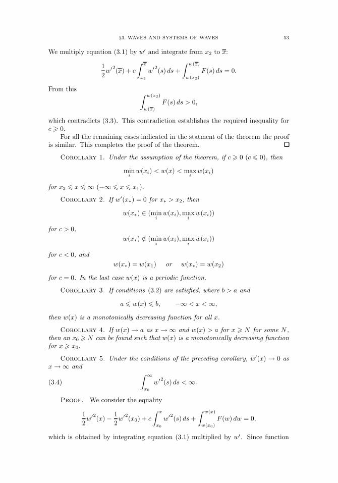
§3. WAVES AND SYSTEMS OF WAVES 53
We multiply equation (3.1) by w′ and integrate from x2 to x:
12w′2(x) + c
∫ x
x2
w′2(s) ds+∫ w(x)
w(x2)
F (s) ds = 0.
From this ∫ w(x2)
w(x)
F (s) ds > 0,
which contradicts (3.3). This contradiction establishes the required inequality forc 0.
For all the remaining cases indicated in the statment of the theorem the proofis similar. This completes the proof of the theorem.
Corollary 1. Under the assumption of the theorem, if c 0 (c 0), then
miniw(xi) < w(x) < max
iw(xi)
for x2 x ∞ (−∞ x x1).
Corollary 2. If w′(x∗) = 0 for x∗ > x2, then
w(x∗) ∈ (miniw(xi),max
iw(xi))
for c > 0,w(x∗) /∈ (min
iw(xi),max
iw(xi))
for c < 0, andw(x∗) = w(x1) or w(x∗) = w(x2)
for c = 0. In the last case w(x) is a periodic function.
Corollary 3. If conditions (3.2) are satisfied, where b > a and
a w(x) b, −∞ < x <∞,
then w(x) is a monotonically decreasing function for all x.
Corollary 4. If w(x) → a as x→∞ and w(x) > a for x N for some N ,then an x0 N can be found such that w(x) is a monotonically decreasing functionfor x x0.
Corollary 5. Under the conditions of the preceding corollary, w′(x) → 0 asx→∞ and
(3.4)∫ ∞
x0
w′2(s) ds <∞.
Proof. We consider the equality
12w′2(x)− 1
2w′2(x0) + c
∫ x
x0
w′2(s) ds+∫ w(x)
w(x0)
F (w) dw = 0,
which is obtained by integrating equation (3.1) multiplied by w′. Since function
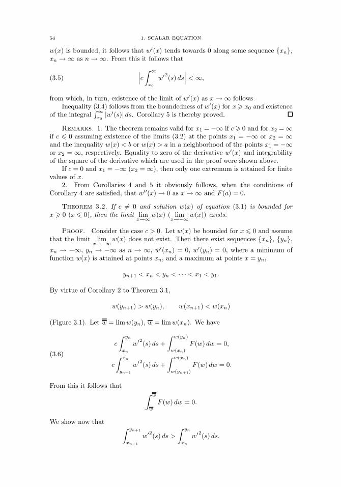
54 1. SCALAR EQUATION
w(x) is bounded, it follows that w′(x) tends towards 0 along some sequence xn,xn →∞ as n→∞. From this it follows that
(3.5)∣∣∣c ∫ ∞
x0
w′2(s) ds∣∣∣ <∞,
from which, in turn, existence of the limit of w′(x) as x→∞ follows.Inequality (3.4) follows from the boundedness of w′(x) for x x0 and existence
of the integral∫∞x0|w′(s)| ds. Corollary 5 is thereby proved.
Remarks. 1. The theorem remains valid for x1 = −∞ if c 0 and for x2 =∞if c 0 assuming existence of the limits (3.2) at the points x1 = −∞ or x2 = ∞and the inequality w(x) < b or w(x) > a in a neighborhood of the points x1 = −∞or x2 = ∞, respectively. Equality to zero of the derivative w′(x) and integrabilityof the square of the derivative which are used in the proof were shown above.
If c = 0 and x1 = −∞ (x2 =∞), then only one extremum is attained for finitevalues of x.
2. From Corollaries 4 and 5 it obviously follows, when the conditions ofCorollary 4 are satisfied, that w′′(x)→ 0 as x→∞ and F (a) = 0.
Theorem 3.2. If c = 0 and solution w(x) of equation (3.1) is bounded forx 0 (x 0), then the limit lim
x→∞w(x) ( lim
x→−∞w(x)) exists.
Proof. Consider the case c > 0. Let w(x) be bounded for x 0 and assumethat the limit lim
x→−∞w(x) does not exist. Then there exist sequences xn, yn,
xn → −∞, yn → −∞ as n → ∞, w′(xn) = 0, w′(yn) = 0, where a minimum offunction w(x) is attained at points xn, and a maximum at points x = yn,
yn+1 < xn < yn < · · · < x1 < y1.
By virtue of Corollary 2 to Theorem 3.1,
w(yn+1) > w(yn), w(xn+1) < w(xn)
(Figure 3.1). Let w = limw(yn), w = limw(xn). We have
(3.6)
c
∫ yn
xn
w′2(s) ds+∫ w(yn)
w(xn)
F (w) dw = 0,
c
∫ xn
yn+1
w′2(s) ds+∫ w(xn)
w(yn+1)
F (w) dw = 0.
From this it follows that ∫ w
w
F (w) dw = 0.
We show now that ∫ yn+1
xn+1
w′2(s) ds >∫ yn
xn
w′2(s) ds.
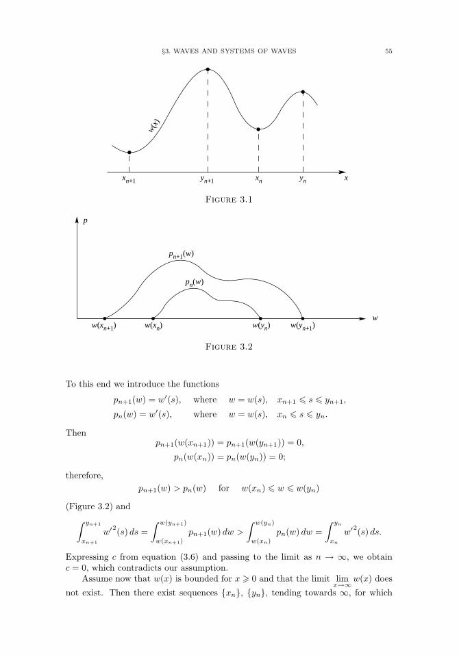
§3. WAVES AND SYSTEMS OF WAVES 55
xn+1 yn+1 xn yn
w(x
)
x
Figure 3.1
p
pn+1(w)
pn(w)
w(xn+1) w(xn) w(yn) w(yn+1)w
Figure 3.2
To this end we introduce the functions
pn+1(w) = w′(s), where w = w(s), xn+1 s yn+1,
pn(w) = w′(s), where w = w(s), xn s yn.
Thenpn+1(w(xn+1)) = pn+1(w(yn+1)) = 0,
pn(w(xn)) = pn(w(yn)) = 0;
therefore,pn+1(w) > pn(w) for w(xn) w w(yn)
(Figure 3.2) and∫ yn+1
xn+1
w′2(s) ds =∫ w(yn+1)
w(xn+1)
pn+1(w) dw >∫ w(yn)
w(xn)
pn(w) dw =∫ yn
xn
w′2(s) ds.
Expressing c from equation (3.6) and passing to the limit as n → ∞, we obtainc = 0, which contradicts our assumption.
Assume now that w(x) is bounded for x 0 and that the limit limx→∞
w(x) does
not exist. Then there exist sequences xn, yn, tending towards ∞, for which
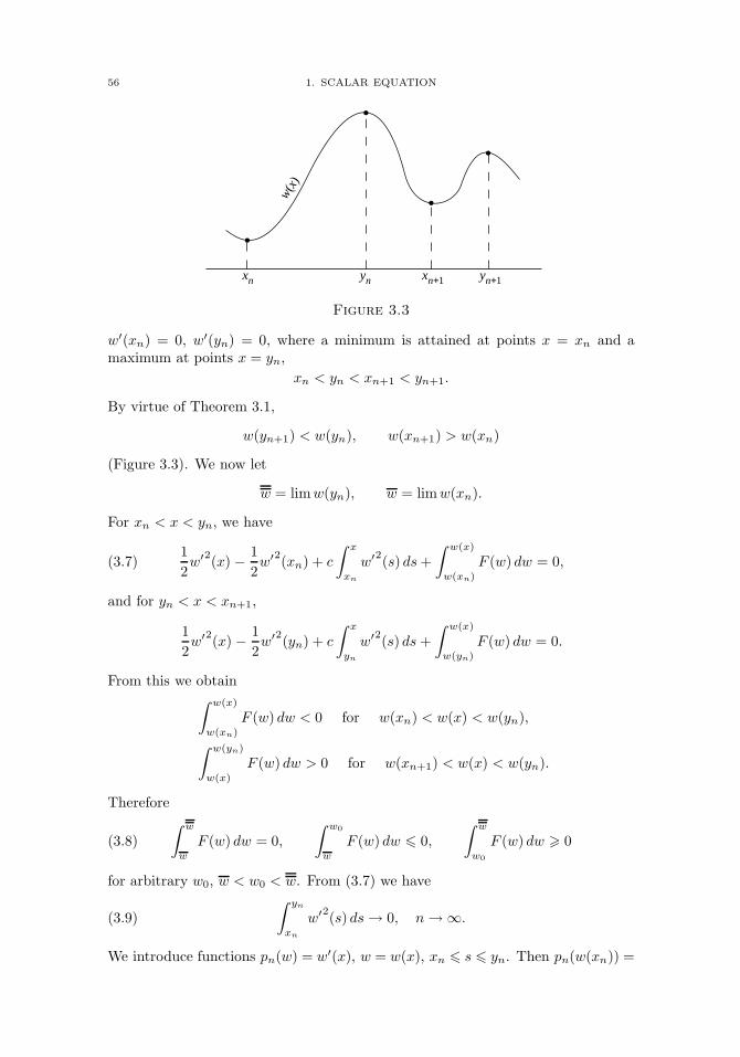
56 1. SCALAR EQUATION
xn+1 yn+1xn ynw
(x)
Figure 3.3
w′(xn) = 0, w′(yn) = 0, where a minimum is attained at points x = xn and amaximum at points x = yn,
xn < yn < xn+1 < yn+1.
By virtue of Theorem 3.1,
w(yn+1) < w(yn), w(xn+1) > w(xn)
(Figure 3.3). We now let
w = limw(yn), w = limw(xn).
For xn < x < yn, we have
(3.7)12w′2(x) − 1
2w′2(xn) + c
∫ x
xn
w′2(s) ds+∫ w(x)
w(xn)
F (w) dw = 0,
and for yn < x < xn+1,
12w′2(x) − 1
2w′2(yn) + c
∫ xyn
w′2(s) ds+∫ w(x)
w(yn)
F (w) dw = 0.
From this we obtain∫ w(x)
w(xn)
F (w) dw < 0 for w(xn) < w(x) < w(yn),∫ w(yn)
w(x)
F (w) dw > 0 for w(xn+1) < w(x) < w(yn).
Therefore
(3.8)∫ w
w
F (w) dw = 0,∫ w0
w
F (w) dw 0,∫ w
w0
F (w) dw 0
for arbitrary w0, w < w0 < w. From (3.7) we have
(3.9)∫ yn
xn
w′2(s) ds→ 0, n→∞.
We introduce functions pn(w) = w′(x), w = w(x), xn s yn. Then pn(w(xn)) =
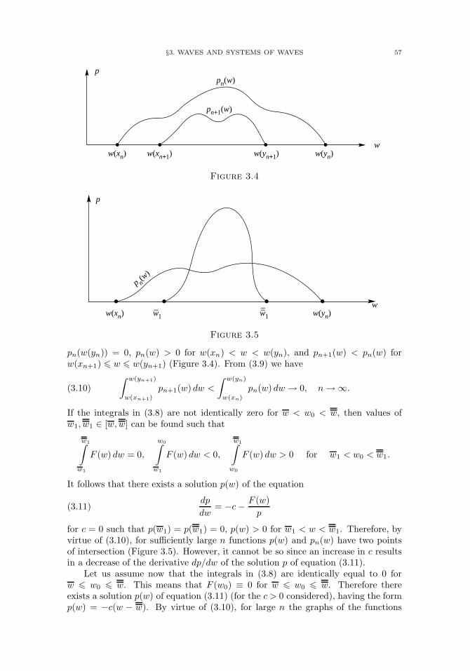
§3. WAVES AND SYSTEMS OF WAVES 57
p
w(xn) w(xn+1) w(yn+1) w(yn)w
pn(w)
pn+1(w)
Figure 3.4
w(xn) w–1 w––
1 w(yn)w
p n(w
)
p
Figure 3.5
pn(w(yn)) = 0, pn(w) > 0 for w(xn) < w < w(yn), and pn+1(w) < pn(w) forw(xn+1) w w(yn+1) (Figure 3.4). From (3.9) we have
(3.10)∫ w(yn+1)
w(xn+1)
pn+1(w) dw <∫ w(yn)
w(xn)
pn(w) dw → 0, n→∞.
If the integrals in (3.8) are not identically zero for w < w0 < w, then values ofw1, w1 ∈ [w,w] can be found such that
w1∫w1
F (w) dw = 0,
w0∫w1
F (w) dw < 0,
w1∫w0
F (w) dw > 0 for w1 < w0 < w1.
It follows that there exists a solution p(w) of the equation
(3.11)dp
dw= −c− F (w)
p
for c = 0 such that p(w1) = p(w1) = 0, p(w) > 0 for w1 < w < w1. Therefore, byvirtue of (3.10), for sufficiently large n functions p(w) and pn(w) have two pointsof intersection (Figure 3.5). However, it cannot be so since an increase in c resultsin a decrease of the derivative dp/dw of the solution p of equation (3.11).
Let us assume now that the integrals in (3.8) are identically equal to 0 forw w0 w. This means that F (w0) ≡ 0 for w w0 w. Therefore thereexists a solution p(w) of equation (3.11) (for the c > 0 considered), having the formp(w) = −c(w − w). By virtue of (3.10), for large n the graphs of the functions
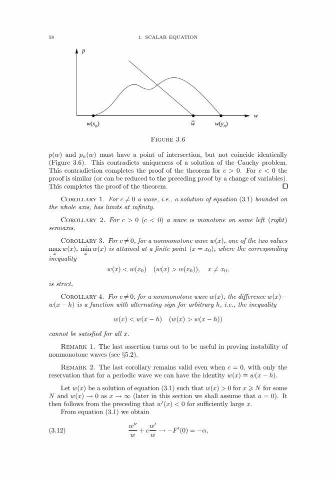
58 1. SCALAR EQUATION
p
w(xn) w––
w(yn)w
Figure 3.6
p(w) and pn(w) must have a point of intersection, but not coincide identically(Figure 3.6). This contradicts uniqueness of a solution of the Cauchy problem.This contradiction completes the proof of the theorem for c > 0. For c < 0 theproof is similar (or can be reduced to the preceding proof by a change of variables).This completes the proof of the theorem.
Corollary 1. For c = 0 a wave, i.e., a solution of equation (3.1) bounded onthe whole axis, has limits at infinity.
Corollary 2. For c > 0 (c < 0) a wave is monotone on some left (right)semiaxis.
Corollary 3. For c = 0, for a nonmonotone wave w(x), one of the two valuesmaxxw(x), min
xw(x) is attained at a finite point (x = x0), where the corresponding
inequality
w(x) < w(x0) (w(x) > w(x0)), x = x0,
is strict.
Corollary 4. For c = 0, for a nonmonotone wave w(x), the difference w(x)−w(x − h) is a function with alternating sign for arbitrary h, i.e., the inequality
w(x) < w(x − h) (w(x) > w(x − h))
cannot be satisfied for all x.
Remark 1. The last assertion turns out to be useful in proving instability ofnonmonotone waves (see §5.2).
Remark 2. The last corollary remains valid even when c = 0, with only thereservation that for a periodic wave we can have the identity w(x) ≡ w(x − h).
Let w(x) be a solution of equation (3.1) such that w(x) > 0 for x N for someN and w(x) → 0 as x → ∞ (later in this section we shall assume that a = 0). Itthen follows from the preceding that w′(x) < 0 for sufficiently large x.
From equation (3.1) we obtain
(3.12)w′′
w+ cw′
w→ −F ′(0) = −α,
§3. WAVES AND SYSTEMS OF WAVES 59
as x→∞. If we differentiate equation (3.1), we then obtain, as x→∞,
(3.13)w′′′
w′ + cw′′
w′ → −α.
We introduce the functions ϕ1(x) = w′(x)w−1(x), ϕ2(x) = w′′(x)[w′(x)]−1. Obvi-ously,
ϕ′1(x) = w
′′(x)w−1(x) − ϕ21(x), ϕ′2(x) = w
′′′(x)[w′(x)]−1 − ϕ22(x).
From (3.12), (3.13) we obtain
(3.14) ϕ′i(x) + cϕi(x) + ϕ
2i → −α (i = 1, 2)
as x→∞.
Theorem 3.3. As x→∞, ϕi(x)→ λ, where λ is a solution of the equation
(3.15) λ2 + cλ+ α = 0.
Proof. We show first that |ϕi(x)| cannot tend to infinity as x→∞. Indeed,let |ϕi(x)| → ∞. Then ψ(x) = ϕ−1
i (x) → 0 as x → ∞. Dividing (3.14) by ϕ2i (x),we obtain ψ′(x)→ 1 as x→∞, which is not possible.
We show that ϕi(x) has a finite limit as x → ∞. Let us assume the contrary.We can then select sequences xn, yn, xn → ∞, yn → ∞, ϕi(xn) → λ1,ϕi(yn) → λ2, λ1 < λ2. Let λ0 satisfy the inequality λ1 < λ0 < λ2 and not be asolution of equation (3.15). If, for example,
λ20 + cλ0 + α > 0,
then for the sequence zn, zn →∞, ϕ(zn) = λ0, ϕ′i(zn) 0, we obtain
ϕ′i(zn) + cϕi(zn) + ϕ
2i (zn) cλ0 + λ20 > −α,
which contradicts (3.14).Thus, ϕi(x)→ λ as x→∞, whence
ϕ′i(x)→ −λ2 − cλ− α.
This limit must be equal to zero in view of the boundedness of ϕi(x). This completesthe proof of the theorem.
Corollary 1. If F (w) ∈ C1[0, 1], w(x) > 0 for sufficiently large x, andw(x)→ 0 as x→∞, then as x→∞ we have one of the following relations:
w′
w→ −c/2 + (c2/4− α)1/2, w′′
w′ → −c/2 + (c2/4− α)1/2,(3.16)
w′
w→ −c/2− (c2/4− α)1/2, w′′
w′ → −c/2− (c2/4− α)1/2,(3.17)
where α = F ′(0), c2/4− α 0.
60 1. SCALAR EQUATION
Corollary 2. If, in the conditions of the preceding corollary, F (w) ∈ r0(0)(i.e., there exists a sequence wn, wn → 0, F (wn) = 0), then as x→∞,
w′
w→ −c, w′′
w′ → −c.
Proof. If sequence xn is such that xn →∞, w(xn) = wn, then
w′′(xn)w′(xn)
= −c− F (w(xn))w′(xn)
= −c.
Since the limit of w′′(x)[w′(x)]−1 as x → ∞ exists, it is then equal to −c. ByL’Hopital’s Rule, w′(x)w−1(x)→−c. This completes the proof of the corollary.
Theorem 3.4. For existence of a solution p(u) of equation (2.7) such thatp(a) = 0 and p(u) < 0 for u > a close to point a, it is necessary that the inequality
(3.18) c ω∗(a)
be satisfied and sufficient that the inequality
(3.19) c > ω∗(a)
be satisfied. If such a solution exists, we then have one of the relations
(3.20)p′(u)→ −c/2 + (c2/4− F ′(a))1/2,
p′(u)→ −c/2− (c2/4− F ′(a))1/2
for u a, where, for F ′(u) ∈ r0(a),
(3.21) p′(u)→ −c (u a).
When conditions (3.19) are satisfied, this solution is unique if F (u) /∈ r+(a) or ifF (u) ∈ r+(a) and the second of conditions (3.20) is satisfied.
Proof. Necessity of condition (3.18) and sufficiency of condition (3.19) followfrom Theorem 2.1. Relations (3.20) and (3.21) follow from Corollaries 1 and 2 ofthe preceding theorem.
Let F (u) ∈ r−(a) and assume that there exist two solutions pi(u) (i = 1, 2)of equation (2.7) satisfying the conditions p1(a) = p2(a) = 0, pi(u) < 0. We setp = p1 − p2 and assume, for definiteness, that p > 0. We obtain
dp
du= k(u)p(u), where k(u) =
F (u)p1(u)p2(u)
.
It follows that p′(u) and p(u) are of different signs for u > a, which is not possiblesince p(a) = 0.
Now let F (u) ∈ r0(a) or F (u) ∈ r+(a) and let the second of conditions (3.20)be satisfied. As above, let p = p1 − p2. We have
k(u)(u− a) = F (u)u− a
u− ap1(a)
u− ap2(a)
−−−→u→a
F ′(a)(c/2 + (c2/4− F ′(a))1/2)2
< 1.
From this we have p′(u) < p(u)(u− a)−1 for a < u < u0 for some u0; consequently,
§3. WAVES AND SYSTEMS OF WAVES 61
p(u) p(u0)(u0 − a)−1(u− a), which contradicts the fact that p(u)(u− a)−1 → 0.This completes the proof of the theorem.
Similarly, we may prove the following theorem.
Theorem 3.5. For existence of a solution p(u) of equation (2.7) such thatp(b) = 0 and p(u) < 0 for u < b close to point b, it is necessary that the inequality
(3.22) c ω∗(b)
be satisfied and sufficient that the inequality
(2.23) c < ω∗(b)
be satisfied. If such a solution exists, we then have one of the relations
(3.24)p′(u)→ −c/2 + (c2/4− F ′(b))1/2,
p′(u)→ −c/2− (c2/4− F ′(b))1/2
as u→ b, where, for F ′(u) ∈ l0(b),
(3.25) p′(u)→ −c (u→ b).
When condition (3.23) is satisfied, this solution is unique if F (u) /∈ l−(b) or ifF (u) ∈ l−(b) and the first of conditions (3.24) is satisfied.
Corollary. Let us assume that the following limit exists and is positive:
αn = limF (u)(u − a)−n (n > 1) as u a.
Then if c > 0, and if the first of relations (3.20) holds for a solution of the system
u′(x) = p(x), p′(x) = −cp(x) + F (u(x)),
then
(3.26) u(x)− a ∼ c1/(n−1)[an(n− 1)x]1/(n−1) as x→∞.
Proof. Since p′(u)→ 0 for u a, then from (2.7) we have F (u)p−1(u)→−c,and, consequently, p(u)(u − a)−n → −c−1an. From this, by L’Hopital’s Rule, asx→∞,
limx(u− a)n−1 = lim(u− a)n[(1 − n)u′(x)]−1 = (n− 1)−1ca−1n ,
and relation (3.26) follows.
3.2. Minimal system of waves. It is convenient to give a definition of asystem of waves in terms of solutions of equation (2.7):
(3.27) p′(u) +F (u)p(u)
+ c = 0.
The converse to equation (3.1) is obvious. As above, we assume that F (a) =F (b) = 0.
Definition 3.1. We shall say that we are given an [a, b]-system of waves ifon the interval [a, b] there is a single-valued continuous function R(u), satisfyingconditions:
1. R(a) = R(b) = 0, R(u) 0 for a u b;
62 1. SCALAR EQUATION
2. If R(u)< 0 for a u1 < u< u2 b, R(u1) =R(u2) = 0, then for some c thereexists a solution p(u) of equation (3.27) such that p(u) = R(u) for u1 < u < u2.
For brevity, in what follows, we shall call R(u) a system of waves.
Definition 3.2. An [a, b]-system of waves R0(u) is called minimal if for anarbitrary [a, b]-system of waves R(u) we have
R0(u) R(u), a u b.It is convenient to introduce the following notation: τc(u;u1, u2) is a solution
p(u) of equation (3.27) satisfying the conditions
p(u) < 0, u1 < u < u2, p(u1) = p(u2) = 0.
Theorem 3.6. For an arbitrary source F (u) there exists an [a, b]-minimalsystem of waves.
Proof. For each u0 ∈ [a, b] let us set
R0(u0) = infp| for some c and u1, u2 : a u1 u0 u2 b, thereexists a solution τc(u;u1, u2) such that p = τc(u0;u1, u2).
If no such solution exists, we set R0(u0) = 0.It is sufficient to show that R(u0) is a system of waves. For this purpose, we
use an estimate of |R0(u)|, which follows from the inequality
(3.28) τ2c (u;u1, u2) 2∫ ba
|F (u)| du, u ∈ [u1, u2].
To prove inequality (3.28) it is sufficient to multiply equation (3.27) by p(u) andintegrate from u1 to u for c 0 and from u to u2 for c > 0.
We note the following estimate for a solution τc(u0;u1, u2) of equation (3.27),passing through the point (u0, p), p < 0:
(3.29) |c| |p|−1max |F (u)|.
This follows from the fact that at point u∗ ∈ (u1, u2), at which function τc(u0;u1,u2) attains a minimum, we have the equality
c = −p−1(u∗)F (u∗).
It follows from the theorem concerning the continuous dependence of a solutionon parameter c, bounded by virtue of (3.29), and on the initial condition, that forsome c1 there exists a function τc1(u; a1, b1) for which
R0(u0) = τc1(u0; a1, b1), c a1 < b1 b.We show that
R0(u) = τc1(u; a1, b1), a1 u b1.Indeed, if this is not so, then for some u1 ∈ [a1, b1], for definiteness, u1 > u0, wehave the inequality
R0(u1) < τc1(u1; a1, b1).
We denote by τc2(u; a2, b2) a solution for which
R0(u1) = τc2(u1; a2, b2), a a2 < b2 b.
§3. WAVES AND SYSTEMS OF WAVES 63
Sinceτc2(u0; a2, b2) τc1(u0; a1, b1),
the equationτc2(u; a2, b2) = τc1(u; a1, b1)
then has a solution u ∈ [u1, u2], and, therefore, a2 > a1. Let c3 < c2, with c3sufficiently close to c2. Then there exists a function
τc3(u; a3, b3), b3 = b2, a3 > a1,
such that
(3.30) τc3(u; a2, b2) < τc2(u; a2, b2), a2 < u < b2.
Inequality (3.30) contradicts the definition of R0(u). This completes the proof ofthe theorem.
From the proof of the theorem we obtain the following
Corollary. R0(u) τc(u; a1, b1) for u ∈ [a1, b1] for arbitrary c and a1, b1 ∈[a, b] for which τc(u; a1, b1) exists.
Theorem 3.7. If R0(u) is the [a, b]-minimal system of waves, and R0(u0) = 0for some u0 ∈ (a, b), then F (u0) = 0.
Proof. We assume the contrary to be true and, for definiteness, let F (u0)> 0.We denote by (a1, b1) an interval such that F (u)> 0 for u∈ (a1, b1), F (a1)=F (b1) =0, and u0 ∈ (a1, b1). By Theorem 2.4, ω∗(u0, b1) = ∞, and, by Theorem 2.3,ω∗(a1, b1) < ∞. Let c > ω∗(a1, b1). From Theorem 2.2, applied to the interval[u0, b1], we conclude that a solution p(u) of equation (3.27) exists, satisfying theconditions p(u) < 0 for u ∈ [u0, b1), p(b1) = 0; and this assertion, applied to theinterval [a1, b1] leads to the equation p(a2) = 0 for some a2 a1. It follows fromthis that R0(u0) < 0, which contradicts our original assumption. If F (u0) < 0, asimilar argument can be made. This completes the proof of the theorem.
Theorem 3.8. Let τc1(u; a1, b1) belong to the [a, b]-minimal system of waves.Then
(3.31) c1 = ω∗(a1, v) = ω∗(u, b1)
for all u, v: a u a1, b1 v b.Proof. We show first that
(3.32) c1 ω∗(a1, b1).
Let c be arbitrary: c < c1. Then, by the usual method (see, for example,Theorem 2.1), it may be proved that there exists a solution p(u) of equation (3.27)such that
p(b1) = 0, p(u) τc1(u; a1, b1) for u ∈ [a1, b1],
where, for at least one point u, the inequality is strict, since c = c1. We havep(a1) < 0; otherwise, τc1(u; a1, b1) would not belong to a minimal system of waves.By virtue of Theorem 2.2 we find that c ω∗(a1, b1), whence (3.32) follows in viewof the arbitrariness of c.
64 1. SCALAR EQUATION
In exactly the same way we can show that
(3.33) c1 ω∗(a1, b1).
From this we find, using (3.32) and (2.18), that
(3.34) c1 = ω∗(a1, b1) = ω∗(a1, b1).
It is now necessary for us to show that
(3.35) ω∗(u, b1) = ω∗(a1, b1)
for all a u a1. Let us assume the contrary:
(3.36) ω∗(u1, b1) < ω∗(a1, b1)
for some u1 ∈ [a, a1). Then, taking c between the values indicated in (3.36), weobtain, by virtue of Theorem 2.2 applied to the interval [a1, b1], that there existsa solution of equation (3.27), satisfying the condition p(u) < 0 for u ∈ [a1, b1),p(b1) = 0, and, by the same proposition applied to the interval [u1, b1], we findthat a continuation of this solution must vanish on the interval [u1, a1). But thiscontradicts the fact that τc1(u; a1, b1) belongs to the minimal system of waves. Ina similar way we may prove equality (3.31) for ω∗. This completes the proof of thetheorem.
Corollary. Let τc1(u; a1, b1) and τc2(u; a2, b2) be two waves from the minimalsystem of waves. Then c1 c2 if b1 a2.
Proof. On the basis of Theorem 3.8,
c1 = ω∗(a1, b2), c2 = ω∗(a1, b2).
It remains now to apply inequality (2.18).We assume that in the system of waves considered there is a right wave and a
left wave, i.e., waves τc1(u; a1, b) and τc2(u; a, b1). It then follows from the resultspresented above that ω∗(a, b) = c1 and ω∗(a, b) = c2. Thus we have arrived at thefollowing interpretation of the functionals introduced in §2: ω∗(a, b) and ω∗(a, b)are the speeds of the left and right waves from the [a, b]-minimal system of waves.In particular, it follows that if ω∗(a, b) = ω∗(a, b), then all waves from the minimalsystem have identical speeds.
The assumption about the presence of a right wave and a left wave is essentialfrom the point of view of applications: its nonfulfillment means that either aninfinite number of waves or an interval of degenerate waves from the minimal systemabut point a or point b.
3.3. Existence of waves. We now obtain conditions for the existence ofwaves. Here, and in what follows, we discuss [a, b]-waves w(x) that satisfy thecondition a w(x) b, and, consequently, by the results of §3.1, monotonicallydecrease.
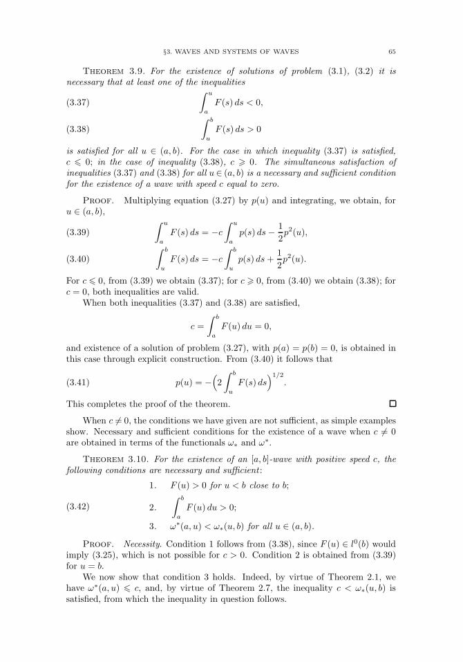
§3. WAVES AND SYSTEMS OF WAVES 65
Theorem 3.9. For the existence of solutions of problem (3.1), (3.2) it isnecessary that at least one of the inequalities∫ u
a
F (s) ds < 0,(3.37) ∫ b
u
F (s) ds > 0(3.38)
is satisfied for all u ∈ (a, b). For the case in which inequality (3.37) is satisfied,c 0; in the case of inequality (3.38), c 0. The simultaneous satisfaction ofinequalities (3.37) and (3.38) for all u∈ (a, b) is a necessary and sufficient conditionfor the existence of a wave with speed c equal to zero.
Proof. Multiplying equation (3.27) by p(u) and integrating, we obtain, foru ∈ (a, b), ∫ u
a
F (s) ds = −c∫ ua
p(s) ds− 12p2(u),(3.39) ∫ b
u
F (s) ds = −c∫ bu
p(s) ds+12p2(u).(3.40)
For c 0, from (3.39) we obtain (3.37); for c 0, from (3.40) we obtain (3.38); forc = 0, both inequalities are valid.
When both inequalities (3.37) and (3.38) are satisfied,
c =∫ b
a
F (u) du = 0,
and existence of a solution of problem (3.27), with p(a) = p(b) = 0, is obtained inthis case through explicit construction. From (3.40) it follows that
(3.41) p(u) = −(2∫ b
u
F (s) ds)1/2
.
This completes the proof of the theorem.
When c = 0, the conditions we have given are not sufficient, as simple examplesshow. Necessary and sufficient conditions for the existence of a wave when c = 0are obtained in terms of the functionals ω∗ and ω∗.
Theorem 3.10. For the existence of an [a, b]-wave with positive speed c, thefollowing conditions are necessary and sufficient :
(3.42)
1. F (u) > 0 for u < b close to b;
2.∫ b
a
F (u) du > 0;
3. ω∗(a, u) < ω∗(u, b) for all u ∈ (a, b).
Proof. Necessity. Condition 1 follows from (3.38), since F (u) ∈ l0(b) wouldimply (3.25), which is not possible for c > 0. Condition 2 is obtained from (3.39)for u = b.
We now show that condition 3 holds. Indeed, by virtue of Theorem 2.1, wehave ω∗(a, u) c, and, by virtue of Theorem 2.7, the inequality c < ω∗(u, b) issatisfied, from which the inequality in question follows.
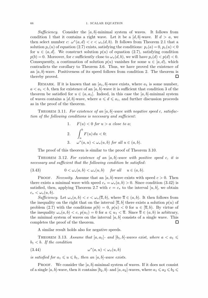
66 1. SCALAR EQUATION
Sufficiency. Consider the [a, b]-minimal system of waves. It follows fromcondition 1 that it contains a right wave. Let it be a [d, b]-wave. If d > a, wethen select number c: ω∗(a, d) < c < ω∗(d, b). It follows from Theorem 2.1 that asolution pc(u) of equation (2.7) exists, satisfying the conditions: pc(a) = 0, pc(u)< 0for u ∈ (a, d]. We construct solution p(u) of equation (2.7), satisfying conditionp(b) = 0. Moreover, for c sufficiently close to ω∗(d, b), we will have pc(d) < p(d)< 0.Consequently, a continuation of solution p(u) vanishes for some u ∈ [a, d), whichcontradicts the corollary to Theorem 3.6. Thus, we have proved the existence ofan [a, b]-wave. Positiveness of its speed follows from condition 2. The theorem isthereby proved.
Remark. If it is known that an [a1, b]-wave exists, where a1 is some number,a < a1 < b, then for existence of an [a, b]-wave it is sufficient that condition 3 of thetheorem be satisfied for u ∈ (a, a1]. Indeed, in this case the [a, b]-minimal systemof waves contains a [d, b]-wave, where a d a1, and further discussion proceedsas in the proof of the theorem.
Theorem 3.11. For existence of an [a, b]-wave with negative speed c, satisfac-tion of the following conditions is necessary and sufficient :
1. F (u) < 0 for u > a close to a;
2.∫ b
a
F (u) du < 0;
3. ω∗(a, u) < ω∗(u, b) for all u ∈ (a, b).
The proof of this theorem is similar to the proof of Theorem 3.10.
Theorem 3.12. For existence of an [a, b]-wave with positive speed c, it isnecessary and sufficient that the following condition be satisfied :
(3.43) 0 < ω∗(a, b) < ω∗(u, b) for all u ∈ (a, b).
Proof. Necessity. Assume that an [a, b]-wave exists with speed c > 0. Thenthere exists a minimal wave with speed c∗ = ω∗(a, b) > 0. Since condition (3.42) issatisfied, then, applying Theorem 2.7 with c = c∗ to the interval [u, b], we obtainc∗ < ω∗(u, b).
Sufficiency. Let ω∗(a, b) < c < ω∗(u, b), where u ∈ (a, b). It then follows fromthe inequality on the right that on the interval [u, b] there exists a solution p(u) ofproblem (2.7) with the conditions p(b) = 0, p(u) < 0 for u ∈ [u, b). By virtue ofthe inequality ω∗(a, b) < c, p(u1) = 0 for a u1 < u. Since u ∈ (a, b) is arbitrary,the minimal system of waves on the interval [a, b] consists of a single wave. Thiscompletes the proof of the theorem.
A similar result holds also for negative speeds.
Theorem 3.13. Assume that [a, a1]- and [b1, b]-waves exist, where a < a1 b1 < b. If the condition
(3.44) ω∗(a, u) < ω∗(u, b)
is satisfied for a1 u b1, then an [a, b]-wave exists.
Proof. We consider the [a, b]-minimal system of waves. If it does not consistof a single [a, b]-wave, then it contains [b2, b]- and [a, a2]-waves, where a1 a2 b2

§3. WAVES AND SYSTEMS OF WAVES 67
b1. On the basis of Theorem 3.8 and inequality (3.44) we have ω∗(b2, b)=ω∗(a2, b)>ω∗(a, a2), which contradicts the corollary to Theorem 3.8. This completes the proofof the theorem.
We have obtained conditions for the existence of waves. We now pose theproblem of classifying all existing [a, b]-waves. The following lemma shows thatnon-uniqueness of a wave is possible only at the expense of different c values.
Lemma 3.1. Equation (2.7), with c given, can have no more than one solutionp(u): p(u) < 0 for u ∈ (a, b), if c 0 and p(b) = 0, or if c 0 and p(a) = 0.
Proof. Let us assume that c 0 and that there exist two different solutionsof the type indicated, p(u) and p1(u). Then from (2.7) we have
(3.45)12[p21(u)− p2(u)] = c
∫ b
u
[p1(s)− p(s)] ds.
Since p1(u) = p(u) for all u ∈ (a, b), we obtain a contradiction in signs in (3.45).Indeed, if, for example, p1(u) > p(u), then the right-hand side in (3.45) is non-negative while the left-hand side is negative. For c 0 the proof is similar. Thiscompletes the proof of the lemma.
Letω∗(a+ 0, b) = lim
uaω∗(u, b), ω∗(a, b− 0) = lim
ubω∗(a, u).
Theorem 3.14. 1. For a source of Type A: if an [a, b]-wave exists, it is uniqueand its speed c may be calculated from the expression
(3.46) c = ω∗(a, b) = ω∗(a, b).
2. For a source of Type B: if an [a, b]-wave exists, then its speed c = 0. If pointa is unstable, we then have the inequality
(3.47) 0 < ω∗(a, b) < ω∗(a+ 0, b),
and a wave exists for those, and only those, speeds c which satisfy the inequality
(3.48) ω∗(a, b) c < ω∗(a+ 0, b).
If point b is unstable, thenω∗(a, b− 0) < ω∗(a, b) < 0,
and a wave exists for those, and only those, speeds c which satisfy the inequality
ω∗(a, b− 0) < c ω∗(a, b).
3. For a source of Type C a wave does not exist.
Proof. 1. From the existence of a wave it follows that a minimal systemof waves consists of a single wave, and, according to Theorem 3.8, its speed iscalculated from (3.46). By the preceding lemma, for a given c the wave is unique.Assume now that a wave exists with speed c1 = c. Let us assume that c1 > c.Then c1 > ω∗(a, b) and, according to Theorem 2.1, there exists a solution p(u) ofequation (2.7) with c = c1, satisfying the conditions
p(a) = 0, p(u) < 0 for u ∈ (a, b].
Thus, for c = c1 there exist two solutions of equation (2.7) with the conditions
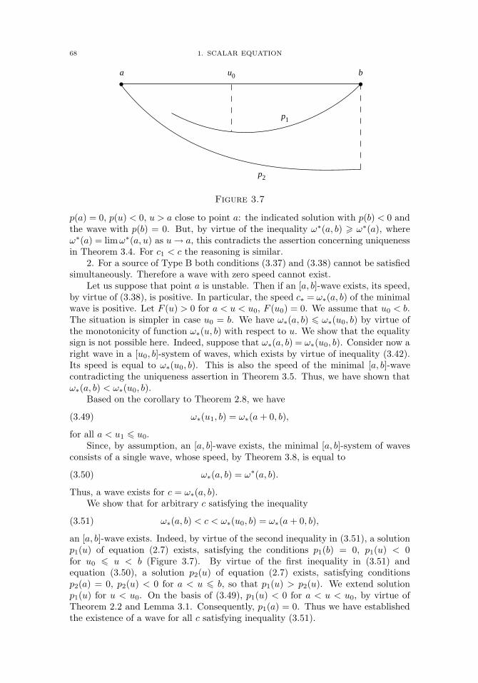
68 1. SCALAR EQUATION
a u0 b
p1
p2
Figure 3.7
p(a) = 0, p(u) < 0, u > a close to point a: the indicated solution with p(b) < 0 andthe wave with p(b) = 0. But, by virtue of the inequality ω∗(a, b) ω∗(a), whereω∗(a) = limω∗(a, u) as u→ a, this contradicts the assertion concerning uniquenessin Theorem 3.4. For c1 < c the reasoning is similar.
2. For a source of Type B both conditions (3.37) and (3.38) cannot be satisfiedsimultaneously. Therefore a wave with zero speed cannot exist.
Let us suppose that point a is unstable. Then if an [a, b]-wave exists, its speed,by virtue of (3.38), is positive. In particular, the speed c∗ = ω∗(a, b) of the minimalwave is positive. Let F (u) > 0 for a < u < u0, F (u0) = 0. We assume that u0 < b.The situation is simpler in case u0 = b. We have ω∗(a, b) ω∗(u0, b) by virtue ofthe monotonicity of function ω∗(u, b) with respect to u. We show that the equalitysign is not possible here. Indeed, suppose that ω∗(a, b) = ω∗(u0, b). Consider now aright wave in a [u0, b]-system of waves, which exists by virtue of inequality (3.42).Its speed is equal to ω∗(u0, b). This is also the speed of the minimal [a, b]-wavecontradicting the uniqueness assertion in Theorem 3.5. Thus, we have shown thatω∗(a, b) < ω∗(u0, b).
Based on the corollary to Theorem 2.8, we have
(3.49) ω∗(u1, b) = ω∗(a+ 0, b),
for all a < u1 u0.Since, by assumption, an [a, b]-wave exists, the minimal [a, b]-system of waves
consists of a single wave, whose speed, by Theorem 3.8, is equal to
(3.50) ω∗(a, b) = ω∗(a, b).
Thus, a wave exists for c = ω∗(a, b).We show that for arbitrary c satisfying the inequality
(3.51) ω∗(a, b) < c < ω∗(u0, b) = ω∗(a+ 0, b),
an [a, b]-wave exists. Indeed, by virtue of the second inequality in (3.51), a solutionp1(u) of equation (2.7) exists, satisfying the conditions p1(b) = 0, p1(u) < 0for u0 u < b (Figure 3.7). By virtue of the first inequality in (3.51) andequation (3.50), a solution p2(u) of equation (2.7) exists, satisfying conditionsp2(a) = 0, p2(u) < 0 for a < u b, so that p1(u) > p2(u). We extend solutionp1(u) for u < u0. On the basis of (3.49), p1(u) < 0 for a < u < u0, by virtue ofTheorem 2.2 and Lemma 3.1. Consequently, p1(a) = 0. Thus we have establishedthe existence of a wave for all c satisfying inequality (3.51).
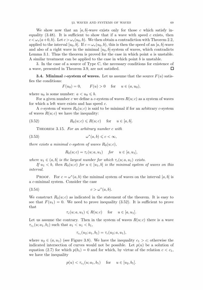
§3. WAVES AND SYSTEMS OF WAVES 69
We show now that an [a, b]-wave exists only for those c which satisfy in-equality (3.48). It is sufficient to show that if a wave with speed c exists, thenc<ω∗(a+0, b). Let c>ω∗(u0, b). We then obtain a contradiction with Theorem 2.2,applied to the interval [u0, b]. If c= ω∗(u0, b), this is then the speed of an [a, b]-waveand also of a right wave in the minimal [u0, b]-system of waves, which contradictsLemma 3.1. Thus the theorem is proved for the case in which point a is unstable.A similar treatment can be applied to the case in which point b is unstable.
3. In the case of a source of Type C, the necessary conditions for existence ofa wave, presented in Theorem 3.9, are not satisfied.
3.4. Minimal c-system of waves. Let us assume that the source F (u) satis-fies the conditions:
F (u0) = 0, F (u) > 0 for u ∈ (a, u0),
where u0 is some number: a < u0 b.For a given number c we define a c-system of waves R(u; c) as a system of waves
for which a left wave exists and has speed c.A c-system of waves R0(u; c) is said to be minimal if for an arbitrary c-system
of waves R(u; c) we have the inequality:
(3.52) R0(u; c) R(u; c) for u ∈ [a, b].
Theorem 3.15. For an arbitrary number c with
(3.53) ω∗(a, b) c <∞,
there exists a minimal c-system of waves R0(u; c),
R0(u; c) = τc(u; a, u1) for u ∈ [a, u1],
where u1 ∈ (a, b] is the largest number for which τc(u; a, u1) exists.If u1 < b, then R0(u; c) for u ∈ [u1, b] is the minimal system of waves on this
interval.
Proof. For c = ω∗(a, b) the minimal system of waves on the interval [a, b] isa c-minimal system. Consider the case
(3.54) c > ω∗(a, b).
We construct R0(u; c) as indicated in the statement of the theorem. It is easy tosee that F (u1) = 0. We need to prove inequality (3.52). It is sufficient to provethat
τc(u; a, u1) R(u; c) for u ∈ [a, u1].
Let us assume the contrary. Then in the system of waves R(u; c) there is a waveτc1(u; a1, b1) such that a1 < u1 < b1,
τc1(u2; a1, b1) = τc(u2; a, u1),
where u2 ∈ (a, u1) (see Figure 3.8). We have the inequality c1 > c; otherwise theindicated intersection of curves would not be possible. Let p(u) be a solution ofequation (2.7) for which p(b1) = 0 and for which, by virtue of the relation c < c1,we have the inequality
p(u) < τc1(u; a1, b1) for u ∈ [u2, b1].
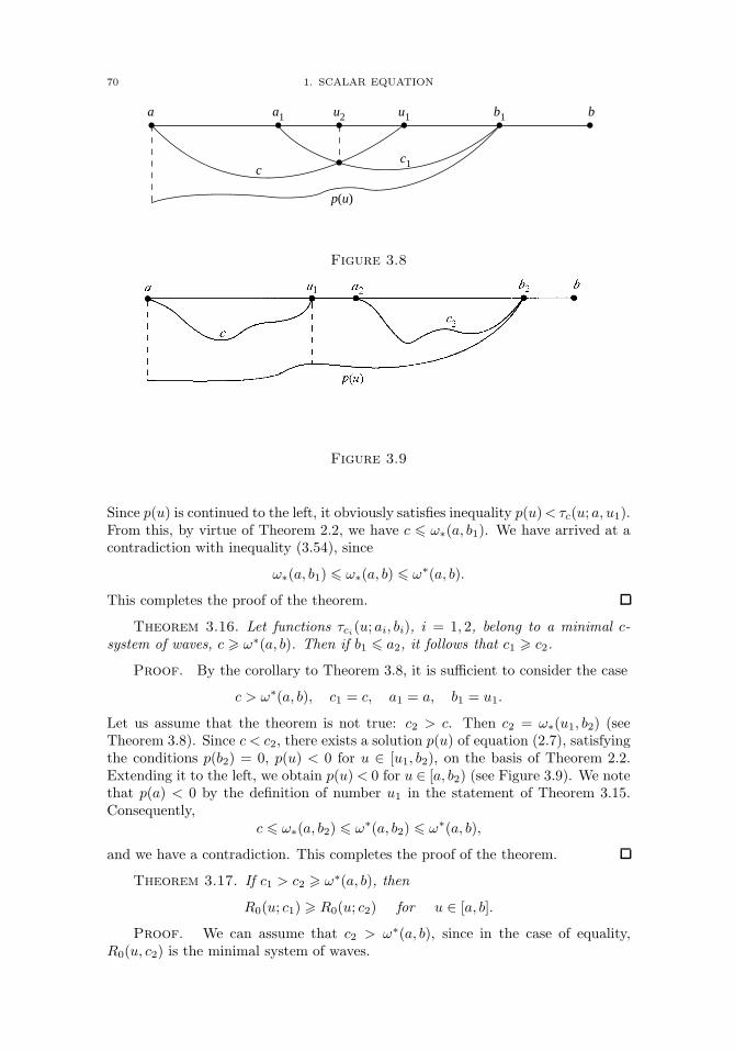
70 1. SCALAR EQUATION
a
c
a1 u2 u1 b1 b
c1
p(u)
Figure 3.8
Figure 3.9
Since p(u) is continued to the left, it obviously satisfies inequality p(u)< τc(u; a, u1).From this, by virtue of Theorem 2.2, we have c ω∗(a, b1). We have arrived at acontradiction with inequality (3.54), since
ω∗(a, b1) ω∗(a, b) ω∗(a, b).
This completes the proof of the theorem.
Theorem 3.16. Let functions τci(u; ai, bi), i = 1, 2, belong to a minimal c-system of waves, c ω∗(a, b). Then if b1 a2, it follows that c1 c2.
Proof. By the corollary to Theorem 3.8, it is sufficient to consider the case
c > ω∗(a, b), c1 = c, a1 = a, b1 = u1.
Let us assume that the theorem is not true: c2 > c. Then c2 = ω∗(u1, b2) (seeTheorem 3.8). Since c < c2, there exists a solution p(u) of equation (2.7), satisfyingthe conditions p(b2) = 0, p(u) < 0 for u ∈ [u1, b2), on the basis of Theorem 2.2.Extending it to the left, we obtain p(u)< 0 for u ∈ [a, b2) (see Figure 3.9). We notethat p(a) < 0 by the definition of number u1 in the statement of Theorem 3.15.Consequently,
c ω∗(a, b2) ω∗(a, b2) ω∗(a, b),
and we have a contradiction. This completes the proof of the theorem.
Theorem 3.17. If c1 > c2 ω∗(a, b), then
R0(u; c1) R0(u; c2) for u ∈ [a, b].
Proof. We can assume that c2 > ω∗(a, b), since in the case of equality,R0(u, c2) is the minimal system of waves.
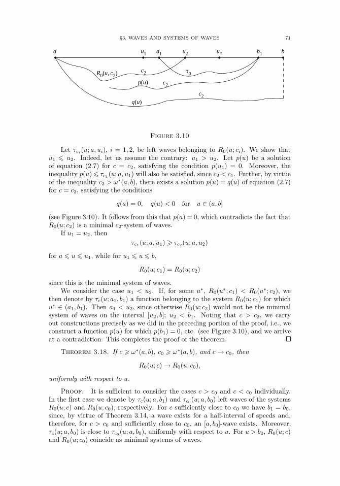
§3. WAVES AND SYSTEMS OF WAVES 71
a u1 a1 u2 u* b1
R0(u, c2) c2
c2
c2q(u)
p(u)
τ0
b
Figure 3.10
Let τci(u; a, ui), i = 1, 2, be left waves belonging to R0(u; ci). We show thatu1 u2. Indeed, let us assume the contrary: u1 > u2. Let p(u) be a solutionof equation (2.7) for c = c2, satisfying the condition p(u1) = 0. Moreover, theinequality p(u) τc1(u; a, u1) will also be satisfied, since c2 < c1. Further, by virtueof the inequality c2 > ω∗(a, b), there exists a solution p(u) = q(u) of equation (2.7)for c = c2, satisfying the conditions
q(a) = 0, q(u) < 0 for u ∈ (a, b]
(see Figure 3.10). It follows from this that p(a) = 0, which contradicts the fact thatR0(u; c2) is a minimal c2-system of waves.
If u1 = u2, thenτc1(u; a, u1) τc2(u; a, u2)
for a u u1, while for u1 u b,
R0(u; c1) = R0(u; c2)
since this is the minimal system of waves.We consider the case u1 < u2. If, for some u∗, R0(u∗; c1) < R0(u∗; c2), we
then denote by τc(u; a1, b1) a function belonging to the system R0(u; c1) for whichu∗ ∈ (a1, b1). Then a1 < u2, since otherwise R0(u; c2) would not be the minimalsystem of waves on the interval [u2, b]; u2 < b1. Noting that c > c2, we carryout constructions precisely as we did in the preceding portion of the proof, i.e., weconstruct a function p(u) for which p(b1) = 0, etc. (see Figure 3.10), and we arriveat a contradiction. This completes the proof of the theorem.
Theorem 3.18. If c ω∗(a, b), c0 ω∗(a, b), and c→ c0, then
R0(u; c)→ R0(u; c0),
uniformly with respect to u.
Proof. It is sufficient to consider the cases c > c0 and c < c0 individually.In the first case we denote by τc(u; a, b1) and τc0(u; a, b0) left waves of the systemsR0(u; c) and R0(u; c0), respectively. For c sufficiently close to c0 we have b1 = b0,since, by virtue of Theorem 3.14, a wave exists for a half-interval of speeds and,therefore, for c > c0 and sufficiently close to c0, an [a, b0]-wave exists. Moreover,τc(u; a, b0) is close to τc0(u; a, b0), uniformly with respect to u. For u > b0, R0(u; c)and R0(u; c0) coincide as minimal systems of waves.
72 1. SCALAR EQUATION
For c c0, R0(u; c) R0(u; c0) and increases with c, and therefore has a limit,which we denote by G(u). Obviously, G(u) R0(u; c0) and is a c0-system of waves.Consequently, G(u) = R0(u; c0) since R0(u; c0) is a minimal c0-system of waves.Thus the theorem is proved.
Minimal c-systems of waves were introduced above for sources of the secondtype on the interval [a, b] (monostable case) for the case in which point a is unstable.It is obvious that for the second case, where point b is unstable, all definitions andproofs are analogous.
For sources of the third type, wherein points a and b are unstable, it is necessaryto introduce somewhat more complex systems of waves, which we refer to as minimalc±-systems. They differ from minimal c-systems in that for them we are given notonly the speed of the wave abutting point a(c+), but also the speed of the waveabutting point b(c−). If we denote the speeds of these waves in the minimal systemof waves by c+0 and c−0 , then the minimal c±-systems of waves will exist for c+ c+0and c− c−0 .
§4. Properties of solutions of parabolic equations
4.1. Existence of solutions of the Cauchy problem and behavior ofsolutions as x→∞. We consider the Cauchy problem for the quasilinear equation
∂v
∂t=∂2v
∂x2+ F (x, t, v),(4.1)
v(x, 0) = f(x),(4.2)
where F (x, t, v) is a bounded continuous function, given for all real x, v, t 0,and satisfying a Lipschitz condition with respect to v and x; f(x) is a boundedpiecewise-continuous function with a finite number of points of discontinuity. Weshall assume that at each discontinuity point x0 the following limiting values exist:
f+(x0) = limxx0
f(x), f−(x0) = limxx0
f(x).
We have the following theorem concerning nonlocal existence of solutions of prob-lem (4.1), (4.2) [Kolm 1].
Theorem 4.1. There exists one and only one function v(x, t), bounded forbounded values of t, which for t > 0 satisfies equation (4.1) and, for t = 0, is equalto f(x) at all points of continuity of this function.
More general results are known concerning nonlocal existence of solutions ofthe Cauchy problem; however, this theorem is sufficient for what follows. Weremark that throughout this chapter our concern is with the existence of a classicalsolution, i.e., we assume that it has continuous derivatives with respect to x up tothe second order inclusive, and a continuous first order derivative with respect to tin an arbitrary domain, where it is defined (but not necessarily in its closure) andcontinuous up to the boundary of the domain of definition at those points where thecorresponding boundary (initial) functions are continuous. A proof of this theorem,and also a proof of Theorem 4.2, is given in Chapter 5 for systems of equations.
§4. PROPERTIES OF SOLUTIONS OF PARABOLIC EQUATIONS 73
Theorem 4.2. Let us assume that the limits
limx→±∞
f(x), limx→±∞,v→v0
F (x, t, v)
exist for arbitrary fixed values v0 and t > 0. Then the function v±(t) = limx→±∞
v(x, t)
is defined and satisfies the equation
dv±dt
= F (±∞, t, v±), v±(0) = f(±∞).
The following theorem concerns a solution of the Cauchy problem
∂u
∂t=∂2u
∂x2+ F (u),(4.3)
u(x, 0) = f(x).(4.4)
Later in this section we assume that F (u) ∈ C2[0, 1],
F (0) = F (1) = 0,
0 f(x) 1 for all x, and we shall use the notation α = F ′(0).In the following two theorems we assume that f(x)→ 0 as x→∞.
Theorem 4.3. Let k and c be given real numbers, and let λ be a real root ofthe equation λ2 − cλ + α = 0. If f(x)eλx → k as x → ∞, then for each t > 0,u(x+ ct, t)eλx → k as x→∞.
Proof. Let us set
u1(x, t) = u(x+ ct, t)eλx, u2(x, t) = u1(x− (c− 2λ)t, t).
Then function u2(x, t) satisfies the equation
∂u2∂t
=∂2u2∂x2
+(λ2 − cλ+ F (u)
u
)u2, u2(x, 0) = f(x)eλx.
According to Theorem 4.2, u2(x, t) → k as x → ∞, whence u1(x, t) → k. Thiscompletes the proof of the theorem.
Corollary 1. If f(x)eλx → k as x → ∞ for some λ, then u(x, t)eλx →ke(λ
2+α)t as x→∞.
The proof is obvious.
Corollary 2. If (ln f(x))/x → −λ as x → ∞, then (lnu(x, t))/x → −λ asx→∞.
Corollary 3. If f(x) = 0 for x x0 for some x0, then (ln u(x, t))/x→ −∞as x→∞.
A proof of the last two corollaries may be obtained from estimates of thefunction f(x) and, consequently, of the solution u(x, t) in terms of an exponentiallydecreasing function.
74 1. SCALAR EQUATION
Later in this subsection we assume that f(x) has a continuous first derivative.In this case it is easily verified that function ω(x, t) = u′(x, t) is a solution of theCauchy problem
∂ω
∂t=∂2ω
∂x2+ F ′(u)ω, ω(x, 0) = f ′(x)
(F ′(u) = dF/du, u′ = ∂u/∂x).
The proof of the following theorem is similar to that of Theorem 4.3.
Theorem 4.4. Let f ′(x)eλx → k as x → ∞, and let λ2 − cλ + α = 0. Then,for each fixed value of t, u′(x+ ct, t)eλx → k as x→∞.
Corollary 1. If f ′(x)eλx → k as x → ∞, then u′(x, t)eλx → ke(λ2+α)t as
x→∞.
Corollary 2. If f(x)eλx → k, f ′(x)/f(x) → −λ as x → ∞, then, for eachfixed value of t, u′(x, t)/u(x, t)→ −λ as x→∞.
The proof of these corollaries is obvious.Here we have considered the behavior of solutions as x → ∞ in some detail
since, in many cases, it determines the behavior of solutions as t→∞.
4.2. Positiveness and the set of zeros of solutions of a linear equation.In this subsection we consider the linear equation
(4.5) Lv = 0,
where
(4.6) Lv =∂v
∂t− ∂
2v
∂x2− a(x, t)∂v
∂x− b(x, t)v.
Equation (4.5) will be considered in a domain D of the (x, t)-plane lying in the strip0 < t < T . Functions a(x, t) and b(x, t) are assumed to be given in D, and, alongwith the derivative ∂a/∂x, are assumed to be bounded and continuous in domainD.We present some theorems on positiveness of solutions of equation (4.5), necessaryfor what follows, and we then use them to study sets of zeros of solutions of thisequation.
We denote by Γ a part of the boundary of domainD lying in the strip 0< t < T ,and by ΓT an interval belonging to the boundary of domain D and lying on theline t = T . Next, following [Fri 1], for an arbitrary point P0 = (x0, t0) ∈ D + ΓT ,we denote by S(P0) a set of points Q in D+ΓT , such that they can be joined withP0 by a simple continuous curve lying in D+ΓT along which coordinate t does notdecrease from Q to P0. As for v(x, t), we assume that it is a bounded function inD, which, together with its derivatives up to the second order with respect to xand up to the first order with respect to t, is continuous in D + ΓT .
Theorem 4.5. If v 0 (v 0) in S(P0), Lv 0 (Lv 0) in S(P0), andv(P0) = 0, then v ≡ 0 in S(P0).
A proof of this theorem is given in [Fri 1].Let Γ0 be the intersection of the closure D of domain D with the axis t= 0. As
for function v, we assume, in addition, that it is continuous in D, except possibly
§4. PROPERTIES OF SOLUTIONS OF PARABOLIC EQUATIONS 75
in a set of points on Γ0 of H-measure 0. Here H is one-dimensional Hausdorffmeasure.
Lemma 4.1. Let D be a bounded set, let Lv 0 in D, and let v(P0) > 0 atsome point P0 = (x0, t0) ∈ D. Then the set of points on Γ with t < t0, at whichfunction v is positive, has positive H-measure.
Proof. Let Γ∗ be the part of set Γ with t < t0. Let us assume that theassertion of the lemma is false: the set γ of points on Γ∗, at which function v ispositive, has H-measure zero. Let k be a number: 0 < k < v(P0). Let w = v − k,and let G be the set of points of domain D for which w > 0.
The closure G of domain G can have an intersection with Γ∗ only on a set ofpoints of discontinuity of function v, and, therefore, this intersection lies on theline t = 0. Indeed, if point P ∈ G ∩ Γ∗ is a point of continuity of function v, thenv(P ) k > 0. Consequently, v(Q) > 0 for points Q lying in some neighborhood ofpoint P in D, and, therefore, the set of points on Γ∗ at which v > 0 has positiveH-measure, which contradicts our assumption.
Consider now the intersection ∆τ of set G with line t = τ . We show that thereexists a positive number ε such that
(4.7)∫∆ε
w(x, ε) dx <∫∆t0
w(x, t0) dx.
Since w(P0) > 0, the right-hand side of (4.7) is then positive, and inequality (4.7)will be proved if we can show that the left-hand side tends towards zero as ε→ 0.Since w(x, t) is bounded in D, it is then sufficient to show that
(4.8) H(∆ε)→ 0 as ε→ 0.
We show this now. Set γ lies on line t = 0 and H(γ) = 0. We cover γ by disks, thesum of whose diameters is less than δ, where δ > 0 is an arbitrary given number.We show that ε > 0 can be specified so that
(4.9) H(∆ε) < δ.
We denote this covering of set γ by K. We show that for some ε,
(4.10) ∆ε ∈ K.
Let us assume the contrary to be true. Then there exists a sequence of values of ε,converging to zero, and a sequence of points Pε ∈ ∆ε, Pε /∈ K. For limit point P∗we have v(P∗) k; this point lies on the line t = 0, so that P∗ ∈ γ, which is notpossible since P∗ is not an interior point of set K. Thus, we have established (4.10),from which (4.9) obviously follows.
Thus we have shown that there exists a number ε > 0 such that inequality (4.7)holds. In what follows, in the course of proving the lemma, we shall assume thatε < t0 is chosen so that (4.7) is valid.
Let Gε be the part of domain G included in the strip ε < t < t0. It is obviousthat the closure Gε of domain Gε belongs to D, and, therefore, function v, togetherwith its derivatives up to the second order with respect to x and up to the firstorder with respect to t, is continuous in Gε. This is obviously also the case forfunction w, so that Lw is a continuous function in Gε.
76 1. SCALAR EQUATION
Temporarily, let us make the following assumption:
(4.11) b 0, −∂a∂x
+ b 0,
in D.From the first of these inequalities it follows that
Lw 0
in Gε. We write Lw in the form
Lw = L0w +(∂a∂x− b)w,
where
(4.12) L0w =∂w
∂t− ∂
∂x
(∂w∂x
+ aw).
From (4.11) we obtain
(4.13) L0w 0
in Gε. Further, we have
(4.14)∫∫Gε
∂w
∂tdx dt =
∫∫Πε
χ∂w
∂tdx dt =
∞∫−∞
dx
t0∫ε
χ∂w
∂tdt,
where Πε is the strip ε < t < t0, and χ is the characteristic function of set Gε.For each x function χ(x, t) is either equal to zero or is the characteristic functionof a finite or countable number of intervals. Function w(x, t) is different from zeroonly on those endpoints of intervals which are on the sets ∆t0 and ∆ε, the latterbeing sections of domain Gε by the lines t = t0 and t = ε. Therefore, from (4.14)it follows that ∫∫
Gε
∂w
∂tdx dt =
∫∆t0
w(x, t0) dx−∫∆ε
w(x, ε) dx > 0.
Here we have taken inequality (4.7) into account. From this, (4.12), and (4.13), itfollows that
(4.15)∫∫Gε
∂
∂x
(∂w∂x
+ aw)dx dt > 0.
On the other hand, calculation of this integral can be carried out directly:
(4.16)∫∫Gε
∂
∂x
(∂w
∂x+ aw
)dx dt =
∫ t0
ε
dt
∫ ∞
−∞χ∂
∂x
(∂w
∂x+ aw
)dx 0.
To prove this inequality we evaluate the inner integral; to this end we considerintervals obtained in sections of domain Gε by the lines t = const, ε < t < t0.Let (α, β) be one such interval. Function w(x, t) is nonnegative in this interval
§4. PROPERTIES OF SOLUTIONS OF PARABOLIC EQUATIONS 77
and vanishes at its endpoints. This latter property follows from the fact that theboundary of Gε has no points in common with Γ. Thus,
∫ β
α
∂
∂x
(∂w
∂x+ aw
)dx =
∂w
∂x
∣∣∣∣β
− ∂w∂x
∣∣∣∣α
0,
since, obviously,
∂w
∂x
∣∣∣∣β
0,∂w
∂x
∣∣∣∣α
0.
The contradiction in signs in (4.15) and (4.16) proves the lemma under theassumption (4.11). If inequality (4.11) does not hold, we then make the substitutionz = v exp(−kt). Obviously, z satisfies the inequality
∂z
∂t− ∂
2z
∂x2− a∂z
∂x− (b − k)z 0.
It is clear that k can be selected so large that, for the operator just obtained,conditions of the form (4.11) are satisfied. The lemma is therefore true for z.Consequently, it is also true for v. This completes the proof of the lemma.
Theorem 4.6. If Lv 0 in D, and v 0 on Γ with the possible exception ofa set of H-measure zero, then v 0 in D.
Proof. First, let us assume that domain D is bounded. Further, let usassume that the theorem is not true: v(P0) < 0 at some point P0 ∈D. For functionu = −v we conclude, on the basis of the lemma, that the intersection with Γ of theset of points where u is positive has positive H-measure, and this contradicts ourhypothesis.
It remains then to consider the case where domain D is unbounded. We changeto a new variable:
(4.17) w(x, t) = v(x, t) sechx.
Then
sechx · Lv = L1w 0 in D,
where
L1w =∂w
∂t− ∂
2w
∂x2− a∂w
∂x− bv,
a(x, t) = a(x, t) + 2 thx,
b(x, t) = 1 + a(x, t) th x+ b(x, t).
It is sufficient to prove the theorem for operator L1 and function w.
78 1. SCALAR EQUATION
We assume at first that
(4.18) b(x, t) 0
in D. We consider the function
z = w + ε, where ε > 0.
Then L1z = L1w − bε 0. From (4.17) it follows that
|w(x, t)| sup0tT
|v(x, t)| sechx −−−−→|x|→∞
0.
Therefore, for |x| = R, where R is a sufficiently large number, z(x, t) > 0. Considernow the domain DR = D ∩ |x| < R. On the boundary of this domain, functionz is positive for t < T , with the exception, possibly, of a set of H-measure zero.Therefore, from what has been proved, z(x, t) ≡ w(x, t) + ε 0 in DR. For eachfixed (x, t) ∈ D we pass to the limit as ε→ 0. We obtain w(x, t) 0.
Thus the theorem has been established under assumption (4.18). The generalcase may be reduced to the case considered, as was done in the proof of the lemma,by the substitution z = w exp(−kt) for k sufficiently large. This completes theproof of the theorem.
A simple consequence of this theorem is the following uniqueness theorem.
Theorem 4.7. If Lv = 0 in D and v = 0 on Γ, except possibly on a set ofH-measure zero, then v = 0 in D.
In our later study of quasilinear equations, the structure of the set of zeros ofsolutions of the linear equation will play a large role. We present these results fora more particular form of domain D, sufficient for what follows.
Consider functions xi(t), i=1, 2, given for t 0, and which satisfy x1(t)<x2(t).We assume that x1(t) is bounded or that x1(t) ≡ −∞; function x2(t) is boundedor x2(t) ≡ +∞. If functions xi(t) are bounded, they are assumed to be continuous.By domain D we shall mean the domain included between the curves xi(t), i= 1, 2,and the lines t = 0, t = T .
The following positiveness theorem for the domain D considered is a directconsequence of Theorems 4.5 and 4.6.
Theorem 4.8. If Lv 0 in D and v 0 on Γ, except, possibly, for a set ofH-measure zero, then v 0 in D. If, moreover, v > 0 at some point of continuity(x1, t1) ∈ Γ, then v > 0 in D + ΓT for t1 t T .
We turn now to the question concerning the structure of the set of zeros ofa solution of the equation Lv = 0. We show, under specified conditions, thatthis is a connected set in the sections ∆(t) of domain D. This will follow fromTheorems 4.9 and 4.10, presented below and clarified in greater detail. At first,we introduce classes A and A0 of functions, given on curve S, homeomorphic tothe interval (0, 1). This homeomorphism determines the ordering of points on S:P1 < P2 if for corresponding points p1 and p2 of the interval (0, 1) we have theinequality p1 p2.
Definition 4.1. Function f , given on S, belongs to class A if, for an arbitrarypoint P0 ∈ S such that f(P0) > 0, the inequality f(P ) > 0 is satisfied for all P ∈ S;
§4. PROPERTIES OF SOLUTIONS OF PARABOLIC EQUATIONS 79
P > P0, and, for an arbitrary point P0 ∈ S such that f(P0) < 0, the inequalityf(P ) < 0 is satisfied for all P ∈ S; P < P0.
Definition 4.2. Function f , given on S, belongs to class A0 if, for an arbitrarypoint P0 ∈ S such that f(P0) > 0, the inequality f(P ) 0 is satisfied for all P ∈ S;P > P0, and for an arbitrary point P0 ∈ S such that f(P0) < 0, the inequalityf(P ) 0 is satisfied for all P ∈ S; P < P0.
Thus, class A0 differs from class A only by the fact that nonstrict inequalitiesare involved. In the definition given above, orientation of S is essential. We indicatenow how curves encountered in the sequel are oriented. Recall that Γ is a part ofthe boundary of domain D for t < T . Obviously, in the case considered, Γ ishomeomorphic to the interval (0, 1). We shall assume curve Γ is oriented so that,as one moves along Γ from point P1 to point P2, P1 < P2, domain D stays to theleft.
We consider sections ∆(t0) of domain D by line t= t0 for 0< t0 <T . Obviously,∆(t0) is homeomorphic to the interval (0, 1). We shall assume that (x1, t0)< (x2, t0)if x1 x2.
Theorem 4.9. Let v be a solution of equation Lv = 0. If v ∈ A0 on Γ, thenv ∈ A in section ∆(t0) of domain D for 0 < t0 < T .
Proof. Let v(x0, t0) > 0 at some point P0 = (x0, t0) ∈ D. We denote byS+(P0) the set of all points Q ∈ D which can be joined to point P0 by a brokenline along which coordinate t does not decrease from Q to P0 and v(x, t) > 0. Wedenote by Λ the set of such broken lines, and we let Γ+ be the part of the boundaryof the set S+(P0) lying in the half-plane t < t0.
We show that if Q ∈ D ∩ Γ+, then v(Q) = 0. Let us suppose that this is notso, i.e., that there exists a point P1 ∈ D ∩ Γ+ such that v(P1) > 0. Consider therectangle
Π = (x, t) : x1 − ε < x < x1 + ε, t1 − ε < t < t1 + ε,
where ε is so small that Π ⊂ D and, in it, v > 0. Let P2 = (x2, t2) be an arbitrarypoint, belonging simultaneously to the sets Π and S+(P0), and let l be a brokenline from Λ, joining P2 and P0. Further, let P3 = (x2, t1 + ε), and let P2P3 be asegment joining points P2 and P3. Applying Theorems 4.5 and 4.6 to the domainbounded by the segment P2P3, the line t = t1 + ε, and the part of the broken linel with t < t1 + ε, we find that P3 ∈ S+(P0) and, consequently, that Π ⊂ S+(P0),which leads to a contradiction. Thus we have shown that the function v vanisheson the set D ∩ Γ+.
Function v, by virtue of Theorem 4.7, is positive on a set of positive measureon Γ+. All points of this set, according to what has been proved, must belong toΓ. Thus there exists a set M of positive H-measure, belonging to Γ+ ∩ Γ, on whichfunction v is positive. Since the set of points of discontinuity of function v hasH-measure zero, we can then select a point P∗ = (x∗, t∗) ∈ M , which is a point ofcontinuity of v and coincides with neither xi(0) nor xi(t0), i = 1, 2.
We show that point P0 can be joined to boundary Γ by a broken line l∗ belongingto domain D, except for one end of it, on which coordinate t does not decreasewhen moving towards point P and on which v > 0. With this in mind, we select aneighborhood Ω of point P∗ in D so small that v > 0 and t < t0 in this neighborhood.Since P∗ ∈ Γ+, there exist a point P1 ∈ S+(P0)∩Ω and a broken line l1 ∈ Λ, joining
80 1. SCALAR EQUATION
P1 with P0. We connect P1 with a point P ∗ ∈ Γ by a segment lying in Ω, exceptfor its endpoint. As such a segment, we take P1P∗, if t∗ = 0, or a segment parallelto the x-axis, if t∗ > 0. We obtain the desired broken line l∗.
Without loss of generality, we can assume that the broken line we have con-structed intersects line t = t0 at only one point, since, otherwise, the single pointof intersection could be attained by a small rotation of the link of the broken linelying on the line t = t0.
We now consider domain G bounded by broken line l∗, a part of curve Γ fort t0, consisting of points P >P ∗, and the part of the line t= t0 for x0 x<x2(t0).Since by a condition of the theorem v ∈ A0 on Γ and v > 0 at point P ∗, it followsthat v 0 for P > P ∗ on Γ. Applying Theorems 4.5 and 4.6 to domain G, we findthat v > 0 on line t = t0 for x0 x < x2(t0).
In exactly the same way we show that if v(P0) < 0, then v < 0 for t = t0,x1(t) < x x0. Consequently, v ∈ A on ∆(t0). This completes the proof of thetheorem.
We present yet another theorem of this kind. Here we impose an additionalrestriction on function v(x, t) if x1(t) or x2(t) is finite. Recall that function v(x, t),together with the derivatives entering into operator L, are assumed to be continuousin domain D +ΓT . Considering the function v(x, t) in the closure D of domain D,we assume the following conditions to be satisfied: 1) function v(x, t) is continuousin D, except, possibly, for a set of points of H-measure zero belonging to an openinterval lying in the intersection of D with the x-axis; 2) if xi(t), i = 1, 2, is finite,then the derivative v′(x, t) exists and is continuous (with respect to D) at eachpoint of the curve x = xi(t), 0 t T , on which v(x, t) = 0.
Remark. In applications to nonlinear equations the requirement for existenceof the derivative v′(x, t) only at points at which v(x, t) = 0 on curves x = xi(t)makes it possible to consider piecewise-continuous initial functions in the Cauchyproblem and does not require existence of the derivative (see Theorem 5.4).
Theorem 4.10. Let v be a solution of the equation Lv = 0 in domain D,satisfying the following condition: if xi(t), i = 1, 2, is finite and v(xi(t), t) = 0,then v′(xi(t), t) > 0 (0 t T ). Then if v ∈ A0 on ∆(0), then v ∈ A on ∆(t) for0 < t < T .
Proof. The case x1(t) ≡ −∞, x2(t) ≡ +∞ was considered in the precedingtheorem.
We begin with the case in which both functions x1(t) and x2(t) are finite. Weassume that for some t ∈ (0, T ) the function v does not belong to class A on ∆(t).We denote by t0 the infimum of all t for which v does not belong to class A on∆(t). Let us assume at first that t0 > 0. Let P1 = (x1(t0), t0), P2 = (x2(t0), t0) (seeFigure 4.1).
We construct neighborhoods Ω1 and Ω2 of points P1 and P2 in D, such that ineach of these neighborhoods either function v is different from zero or v′ > 0.By a condition of the theorem this is possible. Consider, next, the rectangleΠ = Q1Q2S2S1:
(4.19) x1(t0) + ε1 x x2(t0)− ε1, t0 − ε2 t t0 + ε2.
Numbers ε1 > 0 and ε2 > 0 are chosen so small that the following conditions aresatisfied:
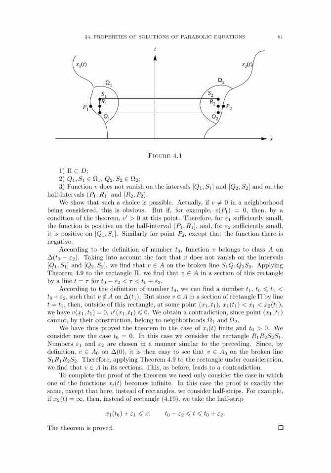
§4. PROPERTIES OF SOLUTIONS OF PARABOLIC EQUATIONS 81
t
x1(t)
P1
S1R1
x2(t)
S2
R2
Q2
Ω1Ω2
P2
x
Q1
Figure 4.1
1) Π ⊂ D;2) Q1, S1 ∈ Ω1, Q2, S2 ∈ Ω2;3) Function v does not vanish on the intervals [Q1, S1] and [Q2, S2] and on the
half-intervals (P1, R1] and [R2, P2).We show that such a choice is possible. Actually, if v = 0 in a neighborhood
being considered, this is obvious. But if, for example, v(P1) = 0, then, by acondition of the theorem, v′ > 0 at this point. Therefore, for ε1 sufficiently small,the function is positive on the half-interval (P1, R1], and, for ε2 sufficiently small,it is positive on [Q1, S1]. Similarly for point P2, except that the function there isnegative.
According to the definition of number t0, function v belongs to class A on∆(t0 − ε2). Taking into account the fact that v does not vanish on the intervals[Q1, S1] and [Q2, S2], we find that v ∈ A on the broken line S1Q1Q2S2. ApplyingTheorem 4.9 to the rectangle Π, we find that v ∈ A in a section of this rectangleby a line t = τ for t0 − ε2 < τ < t0 + ε2.
According to the definition of number t0, we can find a number t1, t0 t1 <t0+ ε2, such that v /∈A on ∆(t1). But since v ∈A in a section of rectangle Π by linet = t1, then, outside of this rectangle, at some point (x1, t1), x1(t1) < x1 < x2(t1),we have v(x1, t1) = 0, v′(x1, t1) 0. We obtain a contradiction, since point (x1, t1)cannot, by their construction, belong to neighborhoods Ω1 and Ω2.
We have thus proved the theorem in the case of xi(t) finite and t0 > 0. Weconsider now the case t0 = 0. In this case we consider the rectangle R1R2S2S1.Numbers ε1 and ε2 are chosen in a manner similar to the preceding. Since, bydefinition, v ∈ A0 on ∆(0), it is then easy to see that v ∈ A0 on the broken lineS1R1R2S2. Therefore, applying Theorem 4.9 to the rectangle under consideration,we find that v ∈ A in its sections. This, as before, leads to a contradiction.
To complete the proof of the theorem we need only consider the case in whichone of the functions xi(t) becomes infinite. In this case the proof is exactly thesame, except that here, instead of rectangles, we consider half-strips. For example,if x2(t) =∞, then, instead of rectangle (4.19), we take the half-strip
x1(t0) + ε1 x, t0 − ε2 t t0 + ε2.
The theorem is proved.
82 1. SCALAR EQUATION
Theorems 4.9 and 4.10 enable us to draw a conclusion concerning connectivityof the set of zeros of solutions of the equation Lv = 0. Indeed, if function v belongsto class A, then, obviously, the set of its zeros is connected (not excluding here theempty set of zeros). Therefore, when the conditions for Theorem 4.9 or 4.10 aresatisfied, we can conclude that the set of zeros of solutions of equation Lv = 0 isconnected in sections ∆(t) of domain D.
4.3. Comparison theorems for quasilinear equations. As a consequenceof the theorems on positiveness of solutions of linear equations, presented in thepreceding section, we obtain comparison theorems for solutions of the Cauchyproblem (4.1), (4.2) [Kolm 1].
Let us assume that functions F (x, t, v) and f(x) satisfy the conditions of§4.1, and, in addition, for simplicity, that F (x, t, v) has continuous and boundedderivatives for −∞ < x < +∞, t 0, and v bounded. Then, for t > 0 and for all x:
1. If F (x, t, v) satisfies the same conditions as F (x, t, v), if v(x, t) is a solutionof the corresponding Cauchy problem, and if F (x, t, v) F (x, t, v), thenv(x, t) v(x, t).
2. If f1(x) f2(x) and vi(x, t), i=1, 2, are solutions with the initial conditionsvi(x, 0) = fi(x), then v1(x, t) v2(x, t).
3. If f(x) 0 and F (x, t, 0) = 0, then v(x, t) 0. If f(x) 1 and F (x, t, 1) = 0,then v(x, t) 1.
4. If f(x) 0, f(x) ≡ 0, and F (x, t, 0) = 0, then v(x, t) > 0.All these properties are obviously satisfied for solutions of the Cauchy prob-
lem (4.3), (4.4). (Here and later we assume that F (u) is a continuously differentiablefunction.) For this case we present two more simple propositions.
5. If f(x) is a nonincreasing function, not identically equal to a constant, thenu(x, t) decreases monotonically with respect to x for each t > 0.
This follows from Theorem 4.8, applied to the difference u(x + h, t) − u(x, t),where for h we can take an arbitrary constant.
6. If f(x) is a twice continuously differentiable function and
f ′′ + F (f) 0,
then u(x, t) is nonincreasing with respect to t for each fixed x.This follows from Theorem 4.8, applied to ∂u/∂t. We refer to f(x) in this case
as an upper function. We define a lower function similarly.If as upper (lower) functions we have f1(x) and f2(x), then the solution u(x, t)
of the Cauchy problem (4.3), (4.4) is nonincreasing (nondecreasing) for f(x) ≡min(f1(x), f2(x)) (f(x) ≡ max(f1(x), f2(x))).
All these propositions carry over in an obvious way to the Cauchy problem
∂u
∂t=∂2u
∂x2+ c∂u
∂x+ F (u),(4.20)
u(x, 0) = f(x),(4.21)
where c is a constant.We note also that for problems (4.3), (4.4) and (4.20), (4.21), if F (0) = F (1) = 0
and 0 f(x) 1, then from estimates of the solution 0 u(x, t) 1 there followestimates of the derivatives u′(x, t), u′′(x, t), and u(x, t), independent of x, t (fort t0 > 0) and the initial condition f(x) (see Chapter 5, §5).
§4. PROPERTIES OF SOLUTIONS OF PARABOLIC EQUATIONS 83
We now turn our attention to the less traditional comparison theorems forquasilinear equations. (These are sometimes referred to as comparison theoremson the phase plane.) These theorems are conveniently formulated for functionsp(u, t), which associate to a solution u(x, t) its derivative u′(x, t). We give a precisedefinition of function p(u, t).
We consider the Cauchy problem (4.3), (4.4), and we assume that the initialcondition f(x) is a bounded piecewise-continuous, piecewise-smooth function witha finite number of points of discontinuity for the function and its derivative, forwhich, at each point, the following limits exist:
limxx0
f(x), limxx0
f(x), limxx0
f ′(x), limxx0
f ′(x).
Moreover let us assume that f(x) is a monotonically nonincreasing function, notidentically equal to a constant. Then for each t > 0, u(x, t) is a monotonicallydecreasing bounded function, continuous along with its derivative u′(x, t). Forarbitrary u, u(+∞, t)< u < u(−∞, t), we set p(u, t) = u′(x, t), where x is such thatu(x, t) = u.
We introduce some notation. If it is required to indicate the dependence on theinitial condition, we shall write u(x, t; f) and p(u, t; f). We write u±(t) or u±(t, f)to denote the function u(±∞, t; f), so that, in particular, u±(0; f) = f(±∞).In certain cases it is convenient also to use the notation fh(x) = f(x + h) andfih(x) = fi(x+ h).
Theorem 4.11. Let functions f1(x) and f2(x) satisfy the conditions givenabove (in the definition of p(u, t)) and
(4.22) 0 f2(+∞) f1(+∞), f1(−∞) f2(−∞) 1.
If f1(x+ h)− f2(x) ∈ A0 (see §4.2) for arbitrary h, then for t > 0
(4.23) p(u, t; f2) p(u, t; f1), u+(t; f1) < u < u−(t; f1).
Proof. Since functions u±(t; fi), i = 1, 2, satisfy equation du/dt = F (u)(see Theorem 4.2), it then follows from inequalities (4.22) that in the intervalI = (u+(t; f1);u−(t, f1)) the function p(u, t; f2) is defined.
For arbitrary preassigned t > 0 and u ∈ I we can select h so that
u(x, t; f1h) = u(x, t; f2) = u.
Function
v(x, t) = u(x, t; f1h)− u(x, t; f2)
satisfies the linear equation (4.5), where a = 0, coefficient b can be easily found,and v(x, 0) ∈ A0. By virtue of Theorem 4.9, v(x, t) ∈ A(t) for t > 0, whenceinequality (4.23) follows. This completes the proof of the theorem.
Before discussing the implications of this theorem, we define function p(u, t)for t = 0, limiting ourselves, for simplicity, to strictly monotonic continuous initialconditions. Let f(+∞) < u < f(−∞), and let x0 be a solution of equationf(x) = u. If the derivative f ′(x) is continuous at point x0, we then set, as before,p(u, 0) = f ′(x0). But if the derivative undergoes a discontinuity at this point, we
84 1. SCALAR EQUATION
shall then consider function p to be many-valued at this value of u and to take onall values between lim
xx0f ′(x) and lim
xx0f ′(x).
Corollary 1. Let the inequalities (4.22) be satisfied. If
(4.24) p(u, 0; f2) < p(u, 0; f1), u+(0; f1) < u < u−(0; f1),
then inequality (4.23) holds for all t > 0.
Remark. At points where the functions p(u, 0; fi) are many-valued, inequal-ity (4.24) is to be understood in the sense that all values of function p(u, 0; f1)are larger than all values of function p(u, 0; f2), although this condition can beweakened for those u for which both functions are many-valued.
Proof. It is sufficient to show that f1(x + h) − f2(x) ∈ A0 for arbitrary h.We show, for example, that inequality f1(x0 + h) > f2(x0) implies the inequality
f1(x+ h) f2(x) for x > x0.
Let us suppose that this is not so, and that for some x1 > x0, f1(x1 + h) < f2(x1).Then an x2 can be found, x0 < x2 < x1, such that f1(x2 + h) = f2(x2) and
limxx2
f ′1(x+ h) limxx2
f ′1(x),
which contradicts inequality (4.24). This establishes the corollary.
We remark that propositions of this type can be formulated also for non-strictlymonotone piecewise-continuous initial conditions (if equation f(x) = u has nosolutions for f(+∞) < u < f(−∞), we then set p(u, 0) = −∞) and also fornonmonotone initial conditions.
Corollary 2. Let χ(x) = 1 for x 0 and χ(x) = 0 for x > 0. Then for eachu, 0 < u < 1, function p(u, t;χ) is monotonically nondecreasing with respect to t.
Proof. By virtue of the theorem for an arbitrary smooth monotonicallydecreasing function f(x), 0 f(x) 1, we have the following inequality for t > 0:
p(u, t;χ) p(u, t; f), u+(t; f) < u < u−(t; f).
Setting f(x) = u(x, t0;χ) for arbitrary t0, we obtain
p(u, t;χ) p(u, t+ t0;χ), 0 < u < 1.
The corollary is thereby established.
The last proposition turns out to be essential in establishing the approach ofsolutions to a wave. Behavior of this kind for a solution with initial function χ(x)was observed in [Kolm 1] and is an important result of this paper.
Up to this point we have been concerned with solutions of the Cauchy problem(4.3), (4.4). It is obvious that all the propositions presented remain valid for theCauchy problem (4.20), (4.21). We now present one of the versions of comparisontheorems on the phase plane for the boundary value problem
∂u
∂t=∂2u
∂x2+ F (u), u(x, 0) = f1(x),(4.25)
u(xi(t), t) = ϕi(t), i = 1, 2,(4.26)
in domain D, consisting of points (x, t) for which x1(t) < x < x2(t), 0 < t < T .
§5. APPROACH TO WAVES AND SYSTEMS OF WAVES 85
Function x1(t), as in §4.2, is continuous and bounded, or x1(t) ≡ −∞; functionx2(t) is continuous and bounded, or x2(t) ≡ ∞.
Theorem 4.12. Let solution u(x, t; f1) of problem (4.25), (4.26), along withits derivative u′(x, t; f1), be continuous in D, and assume also that it decreasesmonotonically with respect to x for each t, 0 t T . Further, let u(x, t; f)be a solution of the Cauchy problem (4.3), (4.4), and assume also that it and itsderivative u′(x, t; f) are continuous and that u(x, t; f) decreases monotonically withrespect to x for 0 t T .
If the following conditions are satisfied,
u+(t; f) < ϕ2(t), ϕ1(t) < u−(t; f), t 0,(4.27)
p(u, 0; f) < p(u, 0; f1), ϕ2(0) u ϕ1(0),(4.28)
p(ϕi(t), t; f) < p(ϕi(t), t; f1), t 0, i = 1, 2,(4.29)
then, for t 0,
(4.30) p(u, t; f) p(u, t; f1), ϕ2(t) u ϕ1(t).
Proof. It is easy to see that function
v(x, t) = u(x, t; f1)− u(x, t; fh)
satisfies the conditions of Theorem 4.10 in domain D for arbitrary h. The rest ofthe proof is carried out as was done in the preceding theorem. This completes theproof of the theorem.
We remark that this theorem can be stated, omitting certain details, in aform traditional for parabolic equations: If inequality (4.30) is satisfied for t < Ton the boundary of domain D∗ of the (u, t)-plane, the latter being defined byϕ2(t) < u < ϕ1(t), 0 < t < T , then it is also satisfied throughout the interior of thedomain. The theorem remains valid if the inequalities (4.28)–(4.30) are reversed.It also admits various generalizations, which we shall not discuss here.
§5. Approach to waves and systems of waves
5.1. Concept concerning approach to a wave and a system of waves.Let w(x) be a wave propagating with speed c, i.e., a monotonically decreasing,twice continuously differentiable function, satisfying the equation
(5.1) w′′ + cw′ + F (w) = 0
and conditions at infinity:
w(−∞) = w−, w(+∞) = w+, w− > w+.
(As has already been mentioned, nonmonotone waves can also be considered. We
86 1. SCALAR EQUATION
shall show that they are unstable and, in this sense, hold no special interest.) Ifu(x, t) is a solution of the Cauchy problem
∂u
∂t=∂2u
∂x2+ F (u),(5.2)
u(x, 0) = f(x),(5.3)
then u(x+ ct, t) obviously satisfies the equation
∂u
∂t=∂2u
∂x2+ c∂u
∂x+ F (u),
and the function w(x) is a stationary solution of this equation.
Definition 5.1. We shall say that solution u(x, t) of problem (5.2), (5.3)approaches a wave uniformly if as t → ∞ we have, uniformly with respect tox ∈ (−∞,∞), the convergence
(5.4) u(x+ ct, t)→ w(x − h),
where h is some number.
We note that the wave w(x) is invariant relative to a translation in x. Thenumber h, appearing in (5.4), depends on the initial conditions (5.3). On the otherhand, it is clear that, making a translation in x in the initial condition, we obtainthe result that the solution u(x, t), as well as its limit with respect to t, is translatedby this amount. Therefore, with no loss of generality, we can fix the wave, assigningto it its value at zero:
(5.5) w(0) = w0,
where w0 is an arbitrary number between w+ and w−, assumed to be given.It turns out to be the case, which we shall show in what follows, that in studying
the convergence of solutions of the Cauchy problem to a wave it is not sufficient toconsider only the uniform approach to a wave. Presently, we shall indicate otherforms of convergence important in the study of waves.
Definition 5.2. We say that solution u(x, t) of problem (5.2), (5.3) approachesa wave in form if, for all sufficiently large t, there exists a unique solution of theequation
(5.6) u(x, t) = w0
(which we denote by x =m(t)) and if we have the following convergence, uniformlywith respect to x:
(5.7) u(x+m(t), t)→ w(x) as t→∞.
Solution u(x, t) of problem (5.2), (5.3) approaches a wave in speed if
(5.8) m′(t)→ c as t→∞.
The descriptive interpretation of these definitions is obvious. In defining the ap-proach in form we displace all curves, representing solutions of problem (5.2), (5.3),in the (x, u)-plane in such a way that for all t they pass through point (0, w0), andsuch curves converge uniformly to a wave. The meaning of convergence in speed is
§5. APPROACH TO WAVES AND SYSTEMS OF WAVES 87
that the speed of the point at which solution u(x, t) of the nonstationary equationhas a given value tends towards the speed of the wave.
The following proposition shows how these kinds of convergence are interre-lated.
Proposition 5.1. 1) Uniform approach of solution u(x, t) of problem (5.2),(5.3) to a wave implies an approach in form and the convergence
(5.9) m(t)− ct→ h as t→∞.
2) Approach to a wave in form implies an approach in speed.3) Approach to a wave in form and the convergence (5.9) implies uniform
approach to a wave.
Proof. Let
(5.10) v(x, t) = u(x+ ct+ h, t).
From (5.4) it follows that
(5.11) v(x, t)→ w(x) as t→∞
uniformly with respect to x. Let δ be an arbitrary small positive number. From (5.5)and monotonicity of the wave, it follows that
w(−δ) > w0, w(δ) < w0.
By virtue of (5.11) we have
v(−δ, t) > w0, v(δ, t) < w0
for all sufficiently large t. This implies existence of a solution x = µ(t) of theequation
(5.12) v(x, t) = w0,
satisfying the condition|µ(t)| < δ.
In view of the arbitrariness of δ, we have
(5.13) µ(t)→ 0 as t→∞.
From (5.10) we now see thatx = m(t) ≡ µ(t) + ct+ h
is a solution of equation (5.6), and we conclude from (5.13) that (5.9) is valid.To prove uniqueness of a solution of equation (5.12), we note, in view of the
monotonicity of wave w, that|w(x) − w0| ρ > 0
outside of interval |x| < 1. Therefore, by virtue of (5.11), there can be no solutionof equation (5.12) outside of this interval for sufficiently large t. Further, since thederivative u′′(x, t) is uniformly bounded (see Chapter 5, §5), the convergence (5.11)then implies the convergence v′(x, t) → w′(x) as t → ∞ and |x| < 1. In addition,w′(x) < 0 (see §3.1). Therefore, v′(x, t) < 0 for |x| < 1 and sufficiently larget. Thus v(x, t) is monotone in x for |x| < 1, and, consequently, the solution ofequation (5.12) is unique.
88 1. SCALAR EQUATION
To complete the proof of the first item of Proposition 5.1, it remains merely toverify that (5.7) holds, i.e.,
(5.14) v(x+ µ(t), t)→ w(x),
uniformly with respect to x. This follows from the fact that v(x + µ(t), t) −w(x + µ(t)) → 0, uniformly with respect to x, as t → ∞, by virtue of (5.11);and w(x + µ(t)) − w(x) → 0, uniformly with respect to x, as t → ∞, by virtueof (5.13).
We turn now to a proof of the second item of Proposition 5.1. Differentiatingequation u(m(t), t) = w0 with respect to t, we obtain
(5.15) m′(t) = −u′′(m(t), t) + F (u(m(t), t))
u′(m(t), t).
Since the convergence (5.7) and the uniform boundedness of the derivatives u′′ andu′′′ (see Chapter 5, §5) imply convergence of the derivatives
u′(m(t), t)→ w′(0), u′′(m(t), t)→ w′′(0),
the relation (5.8) then follows by virtue of (5.15).We turn now to the last item of Proposition 5.1. Let µ(t) = m(t) − ct − h.
Then from (5.9) we obtain (5.13). For function v(x, t), defined by equation (5.10),we have (5.14), by virtue of (5.7). Convergence (5.11) then follows from this andfrom (5.13). The proposition is thereby proved.
We consider two basic kinds of convergence to a wave: uniform convergence andconvergence in form and speed. As shown in [Kolm 1], for the source F (u) and theinitial condition, considered therein, we have convergence to a wave in form andspeed, but not uniform convergence. On the other hand, in later papers (referencesare supplied in the commentary to §6) it was shown that for some other kinds ofsources and initial conditions, we do have uniform approach to a wave.
It is clear from the proposition just proved that the difference between conver-gence in form and uniform convergence may be reduced to the behavior of functionm(t) as t→∞; more precisely, its relationship with ct. We turn our attention nowto the fact that m(t) and ct describe the dependence on time of the displacementof a point with a given value for a solution of the Cauchy problem and for a wave,respectively. In the case of uniform convergencem(t)− ct tends towards a constant,while in the case of convergence in form we can only assert that the derivative ofthis difference tends towards zero. For the source considered in [Kolm 1], theasymptotics of m(t) were found in later studies (see [McK 1, Uch 2]):
m(t) = h+ ct+ k ln t+ · · · ,
where k is a constant, from which the indicated difference is seen explicitly.We make yet another remark concerning the relationship between m(t) and
c. Function m′(t) describes the speed of the displacement of point x, determinedfrom equation (5.6). For this speed we have equation (5.15). For the wave speedwe obtained the minimax representation (see §3.3, Theorem 3.14) in which theexpression used is, in fact, of the same form as the right-hand side of (5.15).According to this representation, if u(x, t) is monotone in x, then the maximum ofthe right-hand side of (5.15), taken over all w0 ∈ (w+, w−) with respect to whichm(t) is determined from (5.6), gives an upper estimate of the speed, while the
§5. APPROACH TO WAVES AND SYSTEMS OF WAVES 89
minimum gives a lower estimate of the speed. (It is necessary here to specify theclass of initial conditions. For example, in case the wave is unique, f(x) can bean arbitrary monotone piecewise-continuous function with corresponding values atinfinity.) Thus, at each instant of time, the wave speed is confined between thesmallest and the largest speeds for the motion of points on a solution profile of theCauchy problem.
In studying convergence of solutions of the Cauchy problem to a wave, com-parison theorems on the phase plane introduced in §4.3 are useful. We considerthe case of monotone solutions u(x, t). Remarks concerning nonmonotone solutionsappear in the commentaries in §6. As in the formulation of comparison theorems,we make use of function p(u, t), which puts the value of the derivative u′(x, t) intocorrespondence with the value of u, where x is determined from the relationshipu(x, t) = u. We denote by p0(u) the corresponding function for a wave. As we didearlier, we set u±(t) = limu(x, t) as x→ ±∞.
We define yet another kind of approach to a wave.
Definition 5.3. We say that a solution u(x, t) of problem (5.2), (5.3) ap-proaches a wave in the phase plane if the convergence
(5.16) p(u, t)→ p0(u) as t→∞
holds for u ∈ (w+, w−), uniform on each closed subset of the interval (w+, w−), and
(5.17) u±(t)→ w± as t→∞.
We shall show below that convergence to a wave in form is equivalent toconvergence on the phase plane. Before giving this proof, we prove an auxiliarylemma.
Lemma 5.1. Let function v0(x) be twice continuously differentiable on theinterval [x1, x2], and let function v(x, t) have a continuous second derivative withrespect to x, uniformly bounded with respect to t. We assume that v′0(x) < 0,v′(x, t)< 0 for x∈ [x1, x2] and all t, and v(x0, t) = v0(x0) = v∗ for some x0 ∈ [x1, x2]and v∗.
Then in order for the convergence
(5.18) v(x, t)→ v0(x), t→∞,
to occur uniformly on an arbitrary interval [y1, y2] embedded in the interval (x1, x2),it is necessary and sufficient that for t sufficiently large the function p(u, t) be definedon an arbitrary interval [u1, u2] embedded in the interval (v0(x2), v0(x1)), and
(5.19) p(u, t)→ p0(u) as t→∞,
uniformly on an arbitrary such interval.
Remark. In the lemma it is not assumed that v(x, t) is a solution of prob-lem (5.2), (5.3) and that v(x) is a wave. Functions p(u, t) and p0(u) are defined asbefore:
p(u, t) = v′(x, t), where u = v(x, t),
p0(u) = v′0(x), where u = v0(x).
Proof. Assume that the convergence (5.18) holds. We take an arbitraryinterval [u1, u2], as described in the statement of the lemma. For t sufficiently large,
90 1. SCALAR EQUATION
function p(u, t) is defined on this interval. By virtue of the uniform boundednessof second derivatives, we have the convergence
(5.20) v′(x, t)→ v′0(x) as t→∞,
uniform on an arbitrary interval [y1, y2], embedded in the interval (x1, x2).Let u0 ∈ [u1, u2]. We show that p0(u0, t)→ p0(u0). For this purpose we denote
by ξ0 and ξ(t) solutions of the equations
v0(x) = u0 and v(x, t) = u0,
respectively. It is clear that ξ(t)→ ξ0. From this and from (5.20) we obtain
p(u0, t) = v′(ξ(t), t)→ v′0(ξ0) = p0(u0),
which is what we wished to prove.Uniform convergence for u∈ [u1, u2] will follow from the point convergence (5.19)
if we can show that the derivatives p′(u, t) are uniformly bounded for large t. Since
p′(u, t) = v′′(x, t)/v′(x, t), u = v(x, t),
boundedness of the derivatives then follows from the negativeness of v′0(x), theconvergence (5.20), and the boundedness of v′′(x, t). This establishes the necessitypart of the proof.
Let us assume the convergence (5.19) is valid. For an arbitrary interval [y1, y2],indicated in the statement of the lemma, functions p(u, t) are defined for sufficientlylarge t on the interval [v0(y2), v0(y1)]. It is easy to see that the following equalitiesare valid:
x− x0 =∫ v0(x)
v∗
du
p0(u), x− x0 =
∫ v0(x,t)
v∗
du
p(u, t), y1 x y2.
From this we obtain∫ v0(x,t)
v0(x)
du
p(u, t)= −
∫ v0(x)v∗
du
p(u, t)+∫ v0(x)
v∗
du
p0(u)
and
(5.21) |v(x, t) − v0(x)| maxu,t
|p(u, t)|∣∣∣∣ ∫ v0(x)
v∗
(1
p(u, t)− 1p0(u)
)du
∣∣∣∣.The uniform convergence (5.18) on the interval [y1, y2] follows from the uniformconvergence (5.19) on the interval [v0(y2), v0(y1)] and the boundedness of the firstfactor on the right in (5.21). This completes the proof of the lemma.
Proposition 5.2. In order for a solution u(x, t) of problem (5.2), (5.3) toapproach a wave in form, it is necessary and sufficient that it approaches a wavein the phase plane.
§5. APPROACH TO WAVES AND SYSTEMS OF WAVES 91
Proof. Letv(x, t) = u(x+m(t), t).
Assume that we have approach to a wave in form, i.e., that
(5.22) v(x, t)→ w(x), t→∞,
uniformly with respect to x, −∞ < x <∞. From this we have
v±(t) = limx→±∞
v(x, t)→ w± as t→∞
and, consequently, the convergence (5.17). Convergence (5.16) is a consequence ofthe preceding lemma.
Let the solution approach a wave in the phase plane. It follows from theconvergence (5.17) that for sufficiently large t the function p(u, t) is defined on anarbitrary interval embedding in the interval (w+, w−). It follows from the precedinglemma that the convergence (5.22) is valid on an arbitrary finite interval. It followsfrom this and from the convergence (5.17) that we have uniform convergence on thewhole axis, since wave w(x) and function v(x, t) are monotone in x. This completesthe proof of the proposition.
We turn now to the problem concerning approach to a system of waves. Recall,from Definition 3.2 in §3.2, that a system of waves was introduced in the phase planein the form of function R(u), the graph of which consists of parts of trajectoriesof waves in the phase plane. It is therefore convenient to begin the definition ofconvergence of solutions of the Cauchy problem (5.2), (5.3) to a system of waveswith convergence in the phase plane. This is completely analogous to Definition 5.3.Let us assume we are given a monotone system of waves R(u) for u ∈ [a, b], i.e.,R(u) 0. Moreover, we consider here only such systems of waves for which theequation R(u0) = 0 implies that F (u0) = 0. We remark that minimal and c-minimalsystems of waves, which will be discussed later, satisfy this condition.
Definition 5.4. We say that the solution u(x, t) of problem (5.2), (5.3) ap-proaches a system of waves in the phase plane if
(5.23) p(u, t)→ R(u) as t→∞, u ∈ (a, b),
uniformly on each closed subset of interval (a, b), and
(5.24) u+(t)→ a, u−(t)→ b as t→∞.
We can also give a definition of approach to a system of waves in form, analogousto Definition 5.2. To do this, we note that a system of waves is a finite or infiniteset of waves, i.e., solutions w of equation (5.1), satisfying the following conditionsat infinities:
(5.25) w(+∞) = u1, w(−∞) = u2,
where u1 u2, whereby, in case u1 = u2, we have a constant function w(x) = u1 = u2for all x. In addition, F (u1) = 0. We shall not include the degenerate wavesw(x)≡ aand w(x) ≡ b in the system of waves since the equations u(x, t) = a and u(x, t) = bcan have no solutions, and, correspondingly, approach to these waves, in the senseindicated above, is undefined.
We denote waves satisfying conditions (5.25) by w(x;u1, u2). As we havealready noted, these waves, represented in the phase plane, constitute the graph of
92 1. SCALAR EQUATION
function R(u). Moreover, the waves-constants are points on the p = 0 axis, wherethese points can occupy an entire interval or set of intervals. For simplicity, weconsider monotone solutions u(x, t) of equation (5.2). Nonmonotone solutions, aswell as nonmonotone waves, will be discussed in the supplement to the chapter (§6).
Definition 5.5. We say that a solution u(x, t) of problem (5.2), (5.3) ap-proaches a system of waves in form if (5.24) is satisfied, and if, for an arbitrarywave w(x;u1, u2) in the system of waves considered, we have the convergence
(5.26) u(x+m(t), t)→ w(x;u1, u2) as t→∞,
uniformly on each finite interval of the x-axis. Here m(t) is a solution x of theequation
(5.27) u(x, t) = u0,
where u0 = u1s+ u2(1− s), s is an arbitrary fixed number from the interval (0, 1).
Of course, a system of waves can consist of a single wave, and then Definition 5.5must coincide with Definition 5.2. Nevertheless, there is a formal difference in thesedefinitions. Namely, in Definition 5.2 uniform convergence is required on the wholeaxis. In Definition 5.5 the question concerns convergence on each finite interval andcondition (5.24). However, recall that we are dealing here with solutions u(x, t),monotone in x, and for approach to a wave both of these definitions are equivalent.
Proposition 5.3. If solution u(x, t) of problem (5.2), (5.3) approaches a sys-tem of waves in the phase plane, then it approaches a system of waves in form.
Proof. For nondegenerate waves w(x;u1, u2), u1 = u2, approaching a systemof waves, Proposition 5.3 follows from Lemma 5.1. Assume, now, that u1 = u2,and, as was specified in the definition of systems of waves, u1 = a, u1 = b.
It is required to show that
(5.28) u(x+m(t), t)→ u1, t→∞,
uniformly with respect to x on each finite interval, where m(t) is the solution ofequation u(x, t) = u1. We select N > 0 arbitrary and we prove uniformity of theconvergence (5.28) on the interval [−N, 0]. For the interval [0, N ] this is done inthe same way.
We consider three cases: the system of waves R(u) under consideration isnegative in some right half-neighborhood of point u1; R(u) ≡ 0 in some righthalf-neighborhood of point u1; R(u) ≡ 0 in the half-neighborhood indicated andthere exists a sequence vn, vn u1, for which R(vn) = 0.
In the first case there exists a wave w(x) from the system of waves, for whichw(+∞) = u1. We denote the solution of the equation
u(x, t) = w0,
where w(+∞) < w0 < w(−∞), by m1(t). Then if we assume that w(0) = w0, thefunction
(5.29) v1(x, t) = u(x+m1(t), t)
tends towards a wave uniformly on each finite interval. We show that this impliesthe convergence (5.28), uniformly on the interval [−N, 0].
§5. APPROACH TO WAVES AND SYSTEMS OF WAVES 93
Let ε > 0. We denote by N1 the solution of the equation
w(x) = u1 + δ/2.
For sufficiently large T we have the inequalities
(5.30) u1 < w(x) − δ v1(x, t) w(x) + δ < u1 + ε
for t > T , N1 x N1 +N , where δ = 0.5(w(N +N1)− u1). From the definitionof m(t) we have
(5.31) u(m(t), t) = u1.
We set
(5.32) x0(t) = m(t)−m1(t).
Then from (5.29), (5.31), and (5.32) we obtain
(5.33) v1(x0(t), t) = u1.
From (5.29), (5.30), and (5.32) it follows that
(5.34) u(N1 +m(t)− x0(t), t) < u1 + ε.
On the other hand, from (5.30) and (5.33) we have
N +N1 < x0(t).
From this, and from (5.34), in view of the monotonicity of u(x, t) with respect tox, we have
u(x+m(t), t) < u1 + ε for x −N, t > T.
From equation (5.31) we conclude that
u(x+m(t), t) u1 for x 0.
Thus we have established the uniform convergence (5.28) on the interval [−N, 0].Assume now that R(u) ≡ 0 for u1 u u1 + δ < b for some δ > 0. We have
−N =
u(−N+m(t),t)∫u1
du
p(u, t).
Since p(u, t)→ 0 uniformly on the interval [u1, u1 + δ], then u(−N +m(t), t)→ u1as t → ∞. As was the case above, the required convergence follows from themonotonicity of u(x, t).
We consider the third case. For arbitrary ε > 0 we can find a u0, u1 < u0 <u1 + ε, such that R(u0) < 0, and, consequently, there exists a wave w(x), from thesystem of waves considered, for which u1 < w(+∞) < u1 + ε. From this point on,the discussion proceeds similarly to what was done in the first case. This completesthe proof of the proposition.
94 1. SCALAR EQUATION
5.2. Source of the first type (bistable case). Throughout this section weconsider piecewise-continuous initial functions with a finite number of points ofdiscontinuity and, for simplicity, monotone. If waves w(x) have the limits w+ andw− as x → ±∞, then an obvious necessary condition for approach to a wave inform is, by virtue of (5.17), that the values f(±∞) must be found in the domainof attraction of points w+ and w− relative to the equation
(5.35)du
dt= F (u)
(see Theorem 4.2). We show here that this necessary condition is also sufficient forapproach to a wave in form and speed for a source of the first type.
Let q(x) be a solution of equation (5.1), monotonically decreasing for x1 < x <x2 and satisfying q′(x1) = q′(x2) = 0. Let ui = q(xi), i = 1, 2 (we assume thatw+ <ui <w−), and introduce function τ(u), given for u2 u u1, which associatesto each value of u the value q′(x), where x is determined from the equation q(x) = u.Let I(w+) and I(w−) denote the domains of attraction of points u=w+ and u=w−with respect to equation (5.35).
Lemma 5.2. For an arbitrary monotone initial condition f(x), f(+∞) ∈I(w+), f(−∞) ∈ I(w−), for sufficiently large t, we have the following inequalityfor the solution of problem (5.2), (5.3):
(5.36) p(u, t) τ(u), u2 u u1.
Proof. Let q1 denote a solution of the equation
w′′ + c1w′ + F (w) = 0,
monotonically decreasing on the interval x3 < x < x4, with derivatives equal tozero at its endpoints, q′1(x3) = q′1(x4) = 0, and q(x3) = u1. Here c1 < c and thedifference c − c1 is sufficiently small. Existence of such a solution follows from asimple analysis of trajectories on the phase plane of the system of equations
(5.37) w′ = p, p′ = −c1p− F (u)
(here we need to take into account the fact that F (u2) < 0). Moreover, if τ1(u)is defined with respect to q1(x) (in the same way that τ(u) is defined with respectto q(x)), then, obviously, τ1(u3) = 0, where u3 = q1(x4), w+ < u3 < u2, andτ1(u) τ(u) for u2 u u1.
Obviously, we can assume that f(x) is a function which is smooth and strictlydecreasing (otherwise, as a new initial condition, we would need to take functionu(x, t0) for arbitrary t0 > 0). Further, since the functions u±(t) (= lim
x→±∞u(x, t))
are defined and tend towards w+ and w−, respectively, we can assume also thatf(+∞) < u3, f(−∞) > u1.
We consider function q(x − ct + h) for x1 x − ct + h x2. It satisfiesequation (5.2) and q′(xi) = 0, i= 1, 2. If q(x+ h) = f(x) for x1 x+ h x2, then,by virtue of Theorem 4.12, if for some value of x
q(x− ct+ h) = u(x, t),
where u(x, t) is a solution of Cauchy problem (5.2), (5.3), we have the inequality
q′(x− ct+ h) u′(x, t).
§5. APPROACH TO WAVES AND SYSTEMS OF WAVES 95
There is also a similar proposition for function q1.Next, we consider a strip on the (x, u)-plane, bounded by the lines u = u1 and
u = u2. We can fill this strip with curves of the form (x, q(x + h)), x1 − h x x2 − h, varying the displacement value h from −∞ to +∞. We vary h from +∞to h0, so that the inequality q(x + h) < f(x) will be satisfied for all the values ofx and h indicated above. Similarly, we fill the half-strip u3 u u1 with curves(x, q1(x + h)), where x3 − h x x4 − h, with h varying from h1 to −∞ andq1(x+ h) > f(x).
We now consider all the constructed functions q(x+ h) and q1(x+ h) as initialconditions for equation (5.2), solutions of which are obtained from them by adisplacement. Since c1 < c, then, after a finite time, the two half-strips constructedabove will be joined and the whole strip u2 u u1 will be filled up; in this strip,based on the aforesaid, we shall have the inequality u′(x, t) max(τ(u), τ1(u)),where u = u(x, t). This completes the proof of the lemma.
Remark. The lemma remains valid if the derivatives q′(xi) are negative. Hereone must require, in addition, that the following inequalities be satisfied:
p(ui, t) < τ(ui), t 0, i = 1, 2.
The lemma just proved is readily generalized by allowing x1 to become −∞and x2 to become +∞. The resulting lemma is then somewhat weaker.
Lemma 5.3. Under the conditions of Lemma 5.2, for arbitrary ε > 0 we canfind a t(ε) such that
p(u, t) τ(u) + ε, u2 u u1,for t t(ε).
Proof. We consider a trajectory of system (5.37) for c1 = c, for which thecorresponding function τ1(u) satisfies the following conditions. It is defined foru4 u u3, τ1(u3) = τ1(u4) = 0, τ1(u) < 0 for u ∈ (u4, u3), the quantities |u1− u3|and |u2 − u4| are sufficiently small,
τ1(u) τ(u) + ε, u ∈ [u2, u1] ∩ [u4, u3].
We consider different cases depending on the values of F (ui), i = 1, 2. CaseF (ui) = 0, i = 1, 2, was considered in Lemma 5.2. Let us assume that F (u1) = 0(consequently, F (u1) > 0) and F (u2) = 0. We take c1 > c. If the difference c1− c issufficiently small, a trajectory leaving the point u = u1, p = 0 then satisfies all theconditions listed. In case F (u1) = 0, F (u2) = 0 the trajectory in question comesinto the point u = u2, p = 0 for c1 < c.
It remains to consider the case F (u1) = F (u2) = 0. If c > 0, then F (u) ∈ l+(u1)(see Theorem 3.10) and a trajectory of system (5.37), leaving the stationary pointu = u1, p = 0, satisfies the required conditions if c1 > c and the difference c1 − c issufficiently small. Analogous constructions may be carried out for the case c < 0,and also c = 0, if F (u) ∈ l+(u1) or F (u) ∈ r−(u2). If c = 0 and F (u) ∈ l−(u1) orF (u) ∈ r+(u2), then a (u2, u1)-wave cannot exist. It remains to consider the casec = 0 and F (u) ∈ l0(u1), F (u) ∈ r0(u2).
By Theorem 3.9 there exist, in this case, in an arbitrary left half-neighborhoodof point u1, points of positiveness of function F (u). We consider all possiblewaves w(x; an, bn) with zero speed for which an, bn ∈ (u2, u1) and F (u) ∈ l+(bn),and corresponding functions τ(u; an, bn). We show that for some sequence bn,
96 1. SCALAR EQUATION
converging to u1, the corresponding sequence an converges to u2. If we can showthis, then we can take function τ(u; an, bn) sufficiently close to τ(u) and carry outthe constructions indicated above for it.
Let us suppose that the stated proposition is not valid and that an → u2 forany sequence. We take an arbitrary value b ∈ (u2, u1) for which F (u) ∈ l+(b) andwe let
a = infu1>bnb
an.
Then a > u2. Indeed, if this is not the case and a= u2, there then exists a sequencean converging to u2. The corresponding sequence bn can also be consideredconvergent to some value b0. If b0 = u1, then this contradicts the supposition made;if b0 < u1, then ∫ b0
u2
F (u) du = 0,
which contradicts the existence of a (u2, u1)-wave.According to the definition of number a there exists a wave w(x; a, b) for some
b b. It is easy to see that for all bn > b we have the inequality an b. Indeed, iffor some bn > b the inequality an < b is satisfied, then∫ b
an
F (u) du < 0,
which contradicts the existence of an (a, b)-wave, since an a.Consider the integral
J =∫ u1
b
F (u) du.
From the existence of a (u2, u1)-wave it follows that J > 0. Let us denote by M
the union of all intervals [an, bn] for bn > b. Since∫ bn
an
F (u) du = 0,
then ∫M
F (u) du = 0.
Since all points at which function F (u) is positive on the interval [b, u1] belongto the set M, it then follows from the last equation that J 0. The resultingcontradiction establishes the proposition.
Thus, structure of function q1(x) has been described in all cases. Further proofis carried out similar to the proof of Lemma 5.3. We need only remark that if q1(x)is defined on a semi-axis or on an axis, then the equation f(x) = q1(x+ h) can havea solution for arbitrary h. However, for |h| sufficiently large, q1(x+ h)− f(x) ∈A0,since we can, without loss of generality, assume that f(x) is a smooth function witha negative derivative and f(+∞) < u2, u1 < f(−∞). A similar remark applies tofunction q(x). This completes the proof of the lemma.
Before stating the main theorem of this section, we give, without proof, onemore simple lemma and we prove a proposition important in the sequel.
§5. APPROACH TO WAVES AND SYSTEMS OF WAVES 97
Lemma 5.4. If solution u(x, t) of the Cauchy problem (5.2), (5.3) approachesin form a monotone function g(x), given on interval x1 x x2, i.e., as t→∞
u(x+m(t), t)→ g(x),
uniformly with respect to x, where m(t) is a solution of the equation
u(x0 +m(t), t) = g(x0), x1 < x0 < x2,
and u(x, t) has derivatives u′, u′′, u′′′, uniformly bounded with respect to x andt t0 > 0, then g(x) is a twice continuously differentiable function and it satisfiesequation (5.1) for some c.
Proposition 5.4. Let the numbers χ+ and χ− belong to the domain of at-traction of the stationary points w+ and w− of equation (5.35), and let χ+ w+,χ− w−. Assume, further, that χ(x) is equal to χ+ for x > 0 and to χ− forx 0. Then function p(u, t;χ) is nonmonotonically nondecreasing on the interval[w+, w−] and converges uniformly on this interval to a minimal system of waves.
Proof. It is easy to see that the functions u±(t;χ) converge to w± mono-tonically. Therefore, we can prove, in exactly the same way as in Corollary 2 toTheorem 4.1, that p(t, u;χ) is monotone nondecreasing. Consequently, it convergesuniformly to some function r(u) on the interval [w+, w−]. It follows from Lemma 5.1and Lemma 5.4 that r(u) is a system of waves. It remains to show that it is aminimal system of waves. Let us suppose the contrary to be so:
(5.38) R0(u0) < r(u0)
for some u0 ∈ (w+, w−) and a minimal system of waves R0(u). Let u0 ∈ (u1, u2),where R0(u1) = R0(u2) = 0, R0(u) < 0 for u ∈ (u1, u2). Then, on the basis ofcomparison theorems in the phase plane (§4), we obtain
p(t, u0;χ) R0(u0),
which, in the limit as t → ∞, contradicts (5.38). The proposition is therebyproved.
Theorem 5.1. Let f(x) be a monotone, piecewise continuous function with afinite number of points of discontinuity. Further, suppose that there exists a uniquemonotone wave w(x), satisfying the conditions at infinity w(±∞) = w±.
In order that solution u(x, t) of the Cauchy problem (5.2), (5.3) approach wavew(x) in form and speed, it is necessary and sufficient that the values f(±∞) belongto the domain of attraction of the points w± with respect to equation (5.35).
Remark. Conditions for uniqueness of a wave with given values at infinityare equivalent to the fact that w± are not points of repulsion on the intervalw+ w w−, i.e., F (u) is a source of the first kind on this interval.
In the statement of the theorem the inequality w+ f(x) w− is not requiredand nonstrict monotonicity of the initial function is allowed.
Proof. Necessity of the condition f(±∞) ∈ I(w±), as already noted at thebeginning of this section, follows from Theorem 4.2.
We now prove sufficiency of this condition. To do this, we verify the con-vergences (5.16) and (5.17). Convergence (5.17) follows, obviously, also from
98 1. SCALAR EQUATION
Theorem 4.2. To prove (5.16) it is sufficient to verify, for arbitrary positive εand δ, sufficiently small, that we can find a value of t0(ε, δ), such that
(5.39) p0(u)− ε p(u, t) p0(u) + ε, w+ + δ u w− − δ, t t0.
The inequality on the right in (5.39) follows from Lemmas 5.2 and 5.3. Functionq(x) and function τ(u), corresponding to it, which are involved in the lemmas, canbe constructed in the following way. On the phase plane of the system of equations
(5.40) w′ = p, p′ = −cp− F (w),
where c is the speed of the wave, we consider trajectories and functions p(u) corre-sponding to them. We take an arbitrary point (u0, p0(u0)+σ), where w+<u0<w−,σ is a small positive number, and we determine function τ(u) on an arc of thetrajectory passing through this point and located in the half-plane p 0. Thenp0(u) < τ(u) at the location where the last function is defined; τ(u) tends towardsp0(u) as σ decreases, uniformly with respect to u, on the interval [w+ + δ, w− − δ],where function τ(u) vanishes at the points u = ui, i = 1, 2, located inside theinterval, i.e., w+ < u2, u1 < w−. This follows from properties of sources of the firsttype on the interval [w+, w−], for which only one trajectory comes into a stationarypoint (see Theorems 3.4 and 3.5).
In proving the inequality on the left in (5.39), we make use of Proposition 5.4,in which we now need to define function χ(x) by the equation
χ(x) =χ+ for x > 0,χ− for x 0,
where χ+ =minw+, f+, χ− =maxw−, f−. Validity of the inequality on the leftin (5.39) follows, by virtue of this proposition, from the fact that a minimal systemof waves in the case considered coincides with a wave and p(t, u;χ) p(t, u; f)for u ∈ [w+ + δ, w− − δ] and sufficiently large t. This completes the proof of thetheorem.
This theorem characterizes fairly completely the behavior of solutions of theCauchy problem in the case of sources of the first type, if a wave exists. Ananalogous theorem holds for a minimal system of waves.
Theorem 5.2. Let function f(x) satisfy the condition of the preceding theorem.Further, let F (u) be a source of the first type on the interval w+ u w−.
In order that the solution u(x, t) of the Cauchy problem (5.2), (5.3) approacha minimal system of waves on this interval, it is necessary and sufficient that thevalues f(±∞) belong to the domain of attraction of points w± with respect to theequation (5.35).
Proof. We must add only one remark here to the proof of the precedingtheorem, involving the “inner” waves of the system of waves, i.e., the wavesw(x;u1, u2), w+ < u1, u2 < w−, u1 = u2. Here, in order to prove the inequality onthe right in (5.39) we can use the inequality
p(t, u; f) p(t, u; f0), u1 u u2,
§5. APPROACH TO WAVES AND SYSTEMS OF WAVES 99
where
f0(x) =
u2 for f(x) u2,f(x) for u1 < f(x) < u2,u1 for f(x) u1,
and the convergence
p(t, u; f0)→ τ(u;u1, u2), t→∞
(τ(u;u1, u2) = w′(x;u1, u2), u = w(x;u1, u2)), which is valid on the basis of thepreceding theorem. This completes the proof of the theorem.
In concluding this section we turn our attention to the question concerninginstability of nonmonotone waves (see [Hag 1]).
Theorem 5.3. A nonmonotone wave w(x) is not stable with respect to smallperturbations from C(−∞,+∞).
Proof. Consider the function
f(x) = max(w(x), w(x − h)),
where h is a sufficiently small number. Then for all x
f(x) w(x), f(x) w(x − h),
and, on the basis of Corollary 4 to Theorem 3.2,
f(x) ≡ w(x), f(x) ≡ w(x − h).
Therefore, f(x) is a lower function and the solution u(x, t) of the Cauchy problem
∂u
∂t=∂2u
∂x2+ c∂u
∂x+ F (u), u(x, 0) = f(x),
where c is the speed of wave w(x), increases monotonically with respect to t. Bythe aforementioned corollary, u(x, t) cannot tend towards w(x− τ) for any value ofτ . This completes the proof of the theorem.
Remark. If wave w(x) has more than one extremum, it is then not stable,even with respect to perturbations with finite support.
5.3. Exponent κ. Before going on to the problem concerning approach toa wave or system of waves for sources of the second and third types, we need tointroduce an exponent characterizing the behavior of the initial function at infinity.This will be done in the present section. Let f(x) be a function given on some semi-axis x x0; we assume that f(x) is positive and tends towards zero as x→∞. Itsbehavior at infinity will be characterized with the aid of function Φ(u), which weassume to be given on the semi-axis u > 0 and monotonically increasing. In thesequel we shall take specific functions for Φ(u), but for the present treatment weuse an arbitrary function Φ(u) with the indicated properties.
100 1. SCALAR EQUATION
Given function f(x) we construct, with the aid of function Φ(u), a symmetricfunction of two variables x1, x2 for x1 > x0, x2 > x0:
fΦ(x1, x2) =Φ(f(x1))− Φ(f(x2))
x1 − x2(x1 = x2).
Definition 5.6.
κ[f ] = limx1,x2→∞
fΦ(x1, x2),
κ[f ] = limx1,x2→∞
fΦ(x1, x2).
If κ[f ] = κ[f ], we say that there exists a strict exponent κ[f ], defined by theequation
κ[f ] = limx1,x2→∞
fΦ(x1, x2).
We present several propositions relating to the exponent κ, defined in this way.
Proposition 5.5. We have the following equalities :
(5.41)
κ[f ] = limx→∞,h→0
fΦ(x+ h, x),
κ[f ] = limx→∞,h→0
fΦ(x+ h, x),
κ[f ] = limx→∞,h→0
fΦ(x+ h, x).
Proof. We prove the first of the equalities (5.41). The second equation isproved in a similar way, while the third is obviously a consequence of the first two.We denote the right side of the first of equalities (5.41) by ν[f ]. It follows directlyfrom the definition that ν[f ] κ[f ]. We prove the opposite inequality. Let thefollowing sequence of numbers be given:
x0 < x1 = ξ1 < ξ2 < · · · < ξn = x2.
Obviously,
(5.42) fΦ(x1, x2) =1
x2 − x1
n−1∑k=1
fΦ(ξk, ξk+1)(ξk+1 − ξk).
From this we obtain, for x1 > N , ξk+1 − ξk < δ,
fΦ(x1, x2) supx>N,|h|<δ
fΦ(x+ h, x),
and, consequently, ν[f ] κ[f ]. The proposition is thereby proved.
From this proposition we readily obtain the following proposition.
§5. APPROACH TO WAVES AND SYSTEMS OF WAVES 101
Proposition 5.6. If f(x) is an absolutely continuous function on the semi-axis x > x0, and Φ(u) has a continuous derivative, then
(5.43)
κ[f ] = limx∈M,x→∞
dΦ(f(x))dx
,
κ[f ] = limx∈M,x→∞
dΦ(f(x))dx
,
κ[f ] = limx∈M,x→∞
dΦ(f(x))dx
,
where M is an arbitrary set of full measure on the semi-axis x > x0, contained inthe set of points on which the derivative of function f(x) exists.
Proposition 5.7. We have the following inequalities :
(5.44) limx→∞
Φ(f(x))x
κ[f ], limx→∞
Φ(f(x))x
κ[f ].
If the strict exponent κ[f ] exists, we then have the limit
(5.45) limx→∞
Φ(f(x))x
= κ[f ].
Proof. Inequalities (5.44) are obtained directly from the definitions, and thelimit (5.45) follows from them.
If, in particular, as Φ(u) we take the function lnu, then this proposition impliesa relationship between the Lyapunov exponent and κ. In particular, if the strictexponent κ exists, then the strict Lyapunov exponent exists and they are equal.
Using the exponent κ, we can compare the behavior of functions at ∞. Thusif we are given two functions f1(x) and f2(x) with the properties indicated and
(5.46) κ[f1] < κ[f2],
then, for all sufficiently large x,
(5.47) f1(x) < f2(x).
Indeed, it follows from (5.44) that
limx→∞
Φ(f1(x))x
< limx→∞
Φ(f2(x))x
,
so that, for sufficiently large x,
Φ(f1(x)) < Φ(f2(x)),
whence (5.47) follows.
The following result, more specific for exponent κ, is needed for the sequel.
Proposition 5.8. If fi(x), i = 1, 2, are two functions, given on the x-axis,positive, nonincreasing, and tending towards zero as x → ∞, and if they satisfyinequality (5.46) at +∞ and inequality f2(−∞)< f1(−∞) at −∞, then there existsa number h0 such that for each h h0 the function
(5.48) f2(x+ h)− f1(x)
belongs to class A on the x-axis.
102 1. SCALAR EQUATION
Proof. Let ε < 0.5(κ[f2]− κ[f1]). Then there exists a number N , such thatfor x1 > N , x2 > N ,
f1Φ(x1, x2) < κ[f1] + ε, f2Φ(x1, x2) > κ[f2]− ε.
It is obvious that for h > 0
f2Φ(x1 + h, x2 + h) > κ[f2]− ε.
Thus, for x1 > x2 > N and h > 0 we have
Φ(f1(x1))− Φ(f1(x2)) < Φ(f2(x1 + h))− Φ(f2(x2 + h)),
orΦ(f2(x1 + h1))− Φ(f1(x1)) > Φ(f2(x2 + h))− Φ(f1(x2)).
This means that if function (5.48) is positive for x = x2, it is then also positive forx= x1 > x2, and if function (5.48) is negative for x= x1, then it is also negative forx = x2 < x1. But, by definition, this means that function (5.48) belongs to class Aon the semi-axis x > N for all h > 0.
We now select number h0 indicated in the statement of the proposition. Let x1and x2 be numbers for which the following inequalities are satisfied: x1 < N < x2,f1(x1) > f2(−∞), f2(x2) < f1(N), and let us set h0 = x2 − x1. Then, as can easilybe verified, for h h0 function (5.48) is negative for x N , and, as was shownabove, belongs to class A for x > N . Consequently, it belongs to class A on thewhole axis. This completes the proof of the proposition.
In the sequel, we shall use exponents κ constructed with respect to two func-tions Φ: lnu and (1− n)−1u1−n (n > 1), and we denote these exponents by κn[f ],κn[f ], and κn[f ] (n 1), where, for n > 1, we assume that Φ(u) = (1− n)−1u1−n,and for n = 1, Φ(u) = lnu. Thus, on the basis of Proposition 5.6, if function f(x)has a bounded derivative, then
(5.49) κn[f ] = limx→∞
f ′(x)fn(x)
, κn[f ] = limx→∞
f ′(x)fn(x)
(n 1).
5.4. Sources of the second and third types (monostable and unstablecases). For sources of the second and third types, waves and systems of waves de-termining the behavior of solutions for large times are nonunique, and the approachof a solution to this or another wave or system of waves depend on the behavior ofthe initial function as x → ∞. This means that for each wave, for example, thereexists a class of initial functions from which a solution approaches this wave. Ifthe aim is not to include the broadest class of functions, it is then fairly simpleto describe the behavior of solutions for the case being considered. In broadeningthe class of initial conditions specific complications appear. We therefore confineourselves not to the most general classes of functions, but to classes which, however,characterize the behavior of solutions practically completely. Results obtained forthe most general classes of functions will be presented in §6.
In this section we shall consider piecewise-continuous initial functions with afinite number of points of discontinuity. As was the case above, we limit ourselveshere to monotone initial conditions. We consider first the case in which wave w(x)exists with the conditions w(±∞) = w± and the source F (u) is a source of thesecond type on interval w+ u w−. In this case waves exist for positive ornegative speeds, depending on the sign of function F (u) close to the points w+ and
§5. APPROACH TO WAVES AND SYSTEMS OF WAVES 103
w−. We shall assume, for example, that a source is positive in a half-neighborhoodof these points (the other case is obtained from this by a change of variables).Then the waves wc(x), wc(±∞) = w± exist for a half-interval (semi-axis) of speedsc0 c < c∗, where 0 < c0 < c∗ +∞ (Theorem 3.14).
We assume that source F (u) satisfies the condition
(5.50) limu→w+
F (u)(u− w+)n
= αn.
Here n 1, and αn is a positive number. Let α = F ′(w+), so that α = α1. It isobvious that for n > 1, α = 0, and, thus, we consider the case when F ′(w+) = 0.
Recall that for a wave with minimal speed c0
(5.51) limx→∞
w′c0(x)
wc0(x) − w+= −c0
2−√c204− α;
for waves with nonminimal speeds c
(5.52) limx→∞
w′c0(x)
(wc0(x) − w+)n= −λn(c),
where we have set
(5.53) λn(c) =αn
c2 +(c2
4 − α)1/2
(Theorem 3.4).We show now that solution u(x, t; f) of the Cauchy problem (5.2), (5.3) ap-
proaches a wave with speed c determined by the behavior of f(x) at +∞.It follows from (5.49) and (5.52) that for waves wc(x) with nonminimal speed
c behavior at +∞ is determined by the exponent κn:
(5.54) κn[wc − w+] = −λn(c).
We formulate a theorem relating to approach to a wave.
Theorem 5.4. Let f(x) w+ for x ∈ (−∞,+∞) and let f(−∞) lie in thedomain of attraction of point w− relative to equation (5.35). Then
1. If f(x) ≡ w+ on some semi-axis x x0 or f(x) > w+ and
(5.55) κn[f − w+] −λn(c0), n 1,
then the solution of the Cauchy problem (5.2), (5.3) approaches minimal wave wc0(x)in form and speed.
2. If f(x) > w+, the exponent κn[f − wn] is strict and
(5.56) κn[f − w+] = −λn(c), n 1,
where c0 < c < c∗, then solution u(x, t; f) approaches wave wc(x) in form and speed.
We preclude the proof of this theorem with the following lemma.
104 1. SCALAR EQUATION
Lemma 5.5. There exists a solution q = q(x) of equation
(5.57) q′′ + cq′ + F (q) = 0
for c0 < c < c∗ on semi-axis x 0, satisfying the following conditions:
w+ q(x) for x 0,(5.58)
q′(x) < 0 for x > 0,(5.59)
lim q(x) = w+ as x→∞,(5.60)
limx→∞
q′(x)(q(x) − w+)n
= −λn(c),(5.61)
q(0) = w∗, q′(0) < 0(5.62)
for arbitrary w∗ w− lying in the domain of attraction of the stationary point w−of equation (5.35), or
(5.63) q(0) = w0, q′(0) = 0
for arbitrary w0 ∈ (w+, w−), sufficiently close to w+ or w−.
Proof. We consider a solution of the system
(5.64) u′ = p, p′ + cp+ F (u) = 0
with the initial condition u = w−, p = −ν, where ν > 0 is a given sufficientlysmall number. On the phase plane the corresponding curve lies between wave pc(u)and the solution of system (5.64), coming into point (w+, 0) in a low direction.Therefore, the curve corresponding to the solution being considered comes intopoint (w+, 0) in a high direction, since only one trajectory comes in a low direction.If w∗ > w−, we then extend this trajectory for u > w− to the point w∗. Since,by hypothesis, F (u) < 0 for all these u, the trajectory so extended then does notintersect the p = 0 axis. Upon making a translation with respect to x, we obtain asolution satisfying conditions (5.58)–(5.62).
In order to construct a solution satisfying condition (5.63), we consider atrajectory of system (5.64) leaving point (w0, 0). If w0 is sufficiently close to w+,then F (w) > 0 for w+ <w w0 and, therefore, this trajectory comes into the point(w+, 0). If w0 is sufficiently close to w−, the trajectory then hits the point (w+, 0)owing to proximity to the trajectory corresponding to wave wc. This establishesthe lemma.
We denote by qc the solution (5.57) with conditions (5.58)–(5.62), by qc thesolution of this equation with conditions (5.58)–(5.61) and (5.63), and by p =τc(u) and p = τc(u) the corresponding trajectories on the phase plane (u, p) ofsystem (5.64).
§5. APPROACH TO WAVES AND SYSTEMS OF WAVES 105
Lemma 5.6. Let c1 and c2 be given numbers: c1 > c2 > c0, and let a numberh0 be found such that the initial function f(x) satisfies the conditions
qc1(x+ h)− f(x) ∈ A0 for x −h,(5.65)
qc2(x− h) > f(x) for x h,(5.66)
for h h0. If w∗ f(−∞), w0 < f(−∞), there then exists a number T (c1, c2)such that
(5.67) p(u, t; f) τ c1(u), w+ u w0,
for t > T (c1, c2) and
(5.68) u(x, t; f) < qc2(x− c2t− h) for t > 0, h h0, x > c2t+ h.
Proof. Functions
(5.69) u1h(x, t) = qc1(x+ h− c1t) and u2h(x, t) = qc2(x− h− c2t)
are solutions of equation (5.2) for t > 0 in the domains
(5.70) x+ h− c1t > 0 and x− h− c2t > 0,
correspondingly, with boundary conditions
u′1h(x, t) = 0 for x = c1t− h,
u2h(x, t) = w∗ for x = c2t+ h.
Functions
(5.71) vih(x, t) = uih(x, t)− u(x, t; f) (i = 1, 2)
are solutions of equation (4.5) for a(x, t) = 0 and b(x, t) selected accordingly. It iseasy to see that in domains (5.70) the conditions for Theorem 4.10 are satisfied forv1h and for Theorem 4.8 for v2h. It is assumed here that h h1, where h1 h0,taken so large that qc1(0) < f(−h) (see Remark before Theorem 4.10).
In accordance with these theorems we find, taking (5.65) and (5.66) intoaccount, that for each t > 0
u1h(x, t)− u(x, t; f) ∈ A (h h1),(5.72)
u2h(x, t)− u(x, t; f) > 0 (h h0),(5.73)
on the semi-axes x > c1t− h and x > c2t+ h. This establishes (5.68).Assume now that u0 is an arbitrary number from the half-open interval (w+, w0].
For each t > 0 we denote by x0 = x0(t) the solution of the equation
(5.74) u0 = u(x0, t; f).
We show that a number T can be found, independent of u0, such that for all t > Tthere exists an h = h(t) h1 for which
(5.75) u0 = u1h(x0, t).
Relation (5.67) obviously follows from this by virtue of (5.72). Thus, to completethe proof of the lemma, it only remains to prove that the choice of T is possible.
106 1. SCALAR EQUATION
We denote by x1(u) and x2(u) solutions of the equations
(5.76) qc1(x1) = u and qc2(x2) = u
for u ∈ (w+, w0]. Obviously, as solution h of equation (5.75) we have the number
(5.77) h = x1(u0)− x0 + c1t.
Since u2h(x2(u0) + h1 + c2t, t) = u0, then, by virtue of inequality (5.73), we have,for each t,
x2(u0) + h1 + c2t x0.
From this and from (5.77) we have
(5.78) h > x1(u0)− x2(u0)− h1 + (c1 − c2)t.
We note that numbers x∗ and u∗ can obviously be found such that qc2(x∗) =qc1(x∗) = u∗ and qc2(x) < qc1(x) for x > x∗. It follows from this that x2(u)− x1(u)is negative for u ∈ (w+, u∗). Therefore, x2(u) − x1(u) is bounded from above forall u ∈ (w+, w0] and, by virtue of (5.78), number T can be chosen so that h h1for t > T . This completes the proof of the lemma.
Lemma 5.7. Let c1 and c2 be given numbers, c0 < c2 < c1 < c∗, and assume thata number h0 can be found such that the initial function f(x) satisfies the conditions
f(x) > qc1(x+ h) for x −h,(5.79)
f(x)− qc2(x − h) ∈ A0 for x h, h h0.(5.80)
If w0 < f(−∞) w∗, then
(5.81) u(x, t; f) > qc1(x+ h− c1t)
for t > 0, h h0, x > c1t− h, and a number T (c1, c2) can be found such that
(5.82) p(u, t; f) τc2(u) for w+ u w0, t T (c1, c2).
Proof. As in the proof of the preceding lemma, we consider functions (5.69).Functions
vih(x, t) = u(x, t; f)− uih(x, t), i = 1, 2,
are solutions of equation (4.5).To the function v1h(x, t) we can apply the corollary to Theorem 4.8 in domain
D bounded by the lines t = 0, x + h − c1t = 0, from whence (5.81) follows. Tofunction v2h(x, t) we apply Theorem 4.9 in domain D bounded by the lines t = 0,x− h− c2t = 0. It follows from this that
(5.83) u(x, t; f)− u2h(x, t) ∈ A (h h0)
on line x > c2t+ h.Let u0 ∈ (w+, w0], x0 being determined from equation (5.74). As in the
preceding lemma, it can be proved that a number T can be found, independentof u0, such that for t > T there exists an h = h(t) h0 for which u2h(x0, t) = u0.

§5. APPROACH TO WAVES AND SYSTEMS OF WAVES 107
It follows from this and from (5.83) that (5.82) is valid. The lemma is therebyestablished.
Lemma 5.8. If f(x) ≡ w+ for x > x0 and f(x0) > w+ or f(x) > w+ and
(5.84) κn[f − w+] −λn(c) for c0 c < c∗,
then
(5.85) limt→∞
κn[u(·, t; f)− w+] −λn(c).
If f(x) > w+ andκn[f − w+] −λn(c) for c0 < c < c
∗,
then
(5.86) limt→∞
κn[u(·, t; f)− w+] −λn(c).
Proof. Consider the case in which f(x) > w+ and (5.84) holds. Let c1 >c2 > c, qc1 , qc2 are solutions of equation (5.57) indicated above. Let us applyProposition 5.8 to the functions f1(x) = f(x), f2(x) = qc1(x) for x > 0 andf2(x) ≡ qc1(0) for x < 0. We find that
qc1(x + h)− f1(x) ∈ A for x > −h, h h0.
Choosing as f2(x) the function qc2(x), we obtain, by virtue of (5.47),
qc2(x − h) > f(x), x h, h h0,
if h0 is sufficiently large. Thus we are into the conditions of Lemma 5.6, sothat (5.67) holds, or
p(u, t; f)un
τc1(u)un
.
Changing over to the variables x, we readily find from this that
κn[u(·, t; f)− w+] κn[qc1 − w+] = −λn(c1),
for t sufficiently large. Thus,
limt→∞
κn[u(·, t; f)− w+] −λn(c1).
As c1 → c, we obtain (5.85).If f(x)≡w+ for x > x0 and f(x0) =w+, then, similarly, we can use Lemma 5.6.
To prove (5.86) we employ Lemma 5.7 in exactly the same way. This completes theproof of the lemma.
Proof of Theorem 5.4. We establish approach to a wave in the phase plane.A consequence of this, as shown in §5.1, is approach to a wave in form and speed.
Let c ∈ [c0, c∗). Consider the case in which either f(x) ≡ w+ for x > x0 andf(x0) > 0, or f(x) > w+ and
κn[f − w+] −λn(c).
We obtain an upper estimate to the solution of the Cauchy problem (5.2), (5.3)
108 1. SCALAR EQUATION
in the phase plane. Namely, we prove that for arbitrary small numbers ε > 0 andδ > 0, there exists a number T = T (ε, δ), such that
(5.87) p(u, t; f) pc(u) + εfor w+ u w− − δ, t > T (ε, δ). We assume that δ is chosen so small thatF (w− − δ) > 0. Through point (w− − δ, p) we draw trajectory τ c1(u), c1 > c, soclose to pc(u) that
(5.88) τ c1(u) pc(u) + ε, w+ u w− − δ.
This trajectory comes into the points (w+, 0) and (w0, 0), where w0 ∈ (w−− δ, w−).We choose number t1 so large that u−(t)>w0 for t t1. Further, we select numbert2 such that
κn[u(·, t; f)− w+] < −λn(c1)
for t t2. This is possible by virtue of Lemma 5.8. We set t0 = max(t1, t2) andwe take f0(x) = u(x, t0; f) as the new initial condition. Applying Proposition 5.8to functions f1(x) = f0(x) and f2(x) = qc1(x) for x > 0, f2(x) ≡ qc1(0) for x < 0,we find that
qc1(x+ h)− f0(x) ∈ A for x −h
for h h0. Further, let c2 ∈ (c, c1). Then, by virtue of the property expressed byinequality (5.47), we obtain
qc2(x − h) > f0(x) for x > h h0,if h0 is sufficiently large. Thus, the conditions of Lemma 5.6 are satisfied, so thatp(u, t; f) = p(u, t − t0; f0) τ c1(u) for w+ u w0 and t − t0 > T (c1, c2).Relation (5.87) then follows from this and from (5.88). Upper estimates have thusbeen obtained.
For c ∈ (c0, c∗) the estimate
(5.89) p(u, t; f) pc(u)− εfor u ∈ [w+, w− − δ], t > T1(ε, δ) is obtained in exactly the same way throughuse of Lemma 5.7. The estimate (5.89), together with the estimate (5.87), yieldsconvergence of the solution of the Cauchy problem to a wave with nonminimal speedc, c0 < c < c∗. In the case of minimal speed c0 we have the upper bound (5.87). Alower bound follows from Proposition 5.4 and Theorem 4.11.
To complete the proof of the theorem we need only consider the case f(x)≡w+
for x x0, f(x) > w+ for x < x0 and x0 is a point of continuity of function f(x).We introduce function fh(x) equal to f(x) for x x0 − h and equal to zero forx > x0 − h. By virtue of what was proved above, for each h > 0 the solution ofthe Cauchy problem (5.2), (5.3) with initial condition fh(x) converges in form to awave. This means that if we denote by mh(t) the solution of the equation
(5.90) u(mh(t), t; fh) = (w+ + w−)/2,
we then have the following equality, uniformly with respect to x on the whole axis:
(5.91) limt→∞
u(x+mh(t), t; fh) = wc0(x).
To obtain a similar result for the original function, we note that
fh(x) f(x) fh(x− h),
§5. APPROACH TO WAVES AND SYSTEMS OF WAVES 109
from which it follows that
(5.92) u(x, t; fh) u(x, t; f) u(x− h, t; fh).
If we denote by m(t) the solution of the equation
u(m(t), t; f) = (w+ + w−)/2,
then from (5.92) and (5.90) we obtain
(5.93) mh(t) m(t) mh(t) + h.
From this inequality, (5.92), and the monotonicity of u with respect to x it followsthat
(5.94)u(x+ h+mh(t), t; fh) u(x+m(t), t; fh) u(x+m(t), t; f)
u(x− h+m(t), t; fh) u(x− h+mh(t), t; fh).
Taking into account the uniform convergence (5.91), and also the convergencewc0(x+h)→ wc0(x) as h→ 0, uniformly with respect to x, we conclude from (5.94)that
limt→∞
u(x+m(t), t; f) = wc(x),
uniformly with respect to x. This completes the proof of the theorem.
We proceed to a theorem on approach to a system of waves.
Theorem 5.5. Let f(x) be a nonincreasing function, f(x) w+ for x ∈(−∞,∞), and let f(−∞) lie in the domain of attraction of point w− relative toequation (5.35). Let c0 be the maximal wave speed on the integral [w+, w−].
Then:1. If f(x) ≡ w+ on some semi-axis x x0 or f(x) > w+ and
κn[f − w+] −λn(c0), n 1,
then the solution u(x, t; f) of the Cauchy problem (5.2), (5.3) approaches the mini-mal system of waves in form and speed.
2. If f(x) > w+, the exponent κn[f − wn] is strict, and
κn[f − w+] = −λn(c), n 1,
where c is an arbitrary number, c > c0, then the solution u(x, t; f) approaches ac-minimal system of waves in form and speed.
Proof. Let w(x; a, b) be an arbitrary wave entering the system of wavesR0(u)under consideration, and let τ(u; a, b) be its representation in the phase plane. Weintroduce function f0(x) which coincides with f(x) for a f(x) b, is equal to a forf(x)<a, and is equal to b for f(x)> b. Then, for arbitrary h, f0(x+h)−f(x) ∈A0,from which it follows by Theorem 4.11 that for t 0
(5.95) p(u, t; f) p(u, t; f0), a u min(b, u−(t)).
We note, from an estimate of the derivatives of solutions of equation (3.27), thatfor an arbitrary given ε only a finite number of waves τ(u; a, b) entering into thegiven system of waves can fail to satisfy the condition τ(u; a, b) > −ε for a u b.
110 1. SCALAR EQUATION
Therefore, it follows from the convergence of p(u, t; f0) to τ(u; a, b) and from (5.95)that for arbitrary ε and δ a number T (ε, δ) can be found such that for t > T (ε, δ)
p(u, t; f) R0(u) + ε, w+ u w− − δ.
An estimate from below of function p(u, t; f) for a minimal system of waves followsfrom Proposition 5.4 and Theorem 4.11.
If we consider a c-minimal system of waves for c > c0, then, as in the proofof the preceding theorem, we introduce functions q(x) and q(x), defined for x 0,satisfying the inequality w+ q, q w−, tending towards w+ as x → +∞,q(0) = w−, q′(0) = 0,
q′(x)(q(x) − w+)n
→ −λn(c1), x→∞,
while q(x) satisfies the same type of relation with c2, where c0 < c1 < c2 < c andc− c1 can be arbitrarily small. For sufficiently large t we obtain
(5.96) p(u, t; f) τ(u), w+ u q(0),where the inequality can be strict, choosing, for necessity, the “lower” trajectoryfrom the bundle of trajectories coming into point (w+, 0) of plane (u, p). Herefunction τ(u) corresponds to q(x) and the indicated trajectory. It follows from thelast inequality and the Remarks to Lemma 5.2 that (5.96) is valid for w+ u u−(t)for sufficiently large t.
If we define function q(x) for x < 0 so that on this semi-axis it is equal tow−, then as is readily verified, function p(u, t; q) will increase monotonically withrespect to t for each u, w+ < u < w−, and will tend towards function R1(u)corresponding to a c1-minimal system of waves. Since p(u, t; f) p(u, t− t0; q) fort t0, w+ u u−(t) for t0 sufficiently large, and R1(u) tends towards R(u) asc1 → c, we have the inequality
p(u, t; f) R(u)− ε, w+ u u−(t),where ε→ 0 as t→∞. This completes the proof of the theorem.
The theorem just proved makes it possible to give a general picture of theasymptotic behavior of solutions of the Cauchy problem (5.2), (5.3) for sources ofthe second type (monostable case). We assume that the initial function f(x) isnonincreasing, that f(+∞) = w+, and that f(−∞) lies in the domain of attractionof point w−. If f(x) =w+ on some semi-axis, then, as the theorem implies, solutionsof the Cauchy problem (5.2), (5.3) as t → ∞ converge to the minimal system ofwaves. Consider now the case where f(x) > w+. Since f(x) is a nonincreasingfunction, then κn[f − w+] 0, which follows directly from the definition of theexponent κ (see §5.3). Let κn[f − w+] < 0. Then if κn[f − w+] −λn(c0),where c0 is the maximal wave speed in the minimal system of waves, then thesolution of problem (5.2), (5.3) converges to a minimal system of waves. But ifκn[f − w+] > −λn(c0), then, obviously, we can find exactly one number c > c0,such that κn[f −w+] = −λn(c), and the solution of the Cauchy problem convergesto a c-minimal system of waves. Recall that, according to Theorem 3.15, such asystem of waves exists for arbitrary c c0.
In this way, we see that under the assumptions made relative to f(x) theasymptotic behavior of solutions of the Cauchy problem (5.2), (5.3), in the case ofsources of the second type, may be described by systems of waves. In fact, this
§6. SUPPLEMENT (ADDITIONS AND BIBLIOGRAPHIC COMMENTARIES) 111
is true even under lesser restrictions on the initial function (see §6). There is ananalogous result for sources of the first type, a consequence of Theorem 5.2.
In this section we go into detail on sources of the second type. Sources of thethird type, where both points w+ and w− are unstable, may be studied in exactlythe same way; therefore we limit the discussion to brief remarks only. We note firstthat there are no waves for such sources (see §3). We can therefore discuss only anapproach to a systems of waves. Here we need to require fulfillment of the conditionf(+∞)=w+, f(−∞)=w−. Along with the exponent κ characterizing the behaviorof function f(x) at +∞, it is necessary also to introduce an analogous exponentdescribing the behavior of f(x) at −∞. One must also define analogous c±-minimalsystems of waves. (For such wave systems c+ is the speed of an (a, ·)-wave, c− isthe speed of a (·, b)-wave.) Then, depending on the values of the exponents κ of thefunctions f −w+ and w− − f at +∞ and −∞, respectively, we obtain an approachto the corresponding systems of waves.
§6. Supplement (Additions and bibliographic commentaries)
Wave solutions described by scalar parabolic equations
(6.1)∂u
∂t=∂2u
∂x2+ F (u)
were first considered in papers by Fisher [Fis 1] and by Kolmogorov, Petrovskiy, andPiskunov [Kolm 1] in connection with biological problems concerning propagationof a dominant gene. In [Kolm 1] for a positive source (F (u) > 0, for 0 < u < 1,F (0) = F (1) = 0) with the additional condition
(6.2) F ′(u) F ′(0) for 0 u 1,
the existence of waves was proved for all speeds c c0. The minimal speed of awave in the given case was calculated explicitly and was found equal to 2(F ′(0))1/2.For an initial condition of a particular form
(6.3) u(x, 0) = f(x),
where f(x) = 1 for x 0, f(x) = 0 for x > 0, approach of a solution of theCauchy problem (6.1), (6.3) to a wave with minimal speed, and in form andspeed the absence of a uniform approach was proved. Zel′dovich and Frank-Kamenetsky [Zel 2] showed that equation (6.1) can describe propagation of a waveof combustion of gases (see source in Figure 1.3) and they presented a method of de-termining approximately the speed of the wave for problems of combustion (narrowreaction zone method). In [Baren 2] stability of a wave to small perturbations wasestablished and the concept of stability with shift (see Chapter 5) was introduced.In [Kan 1, 3] studies were made of the problem of the stability of a wave and ofthe approach to a wave for sufficiently general initial conditions in the case of apositive source and for a source satisfying the conditions
F (u) 0 for 0 < u < u0 < 1,
F (u) > 0 for u0 < u < 1,∫ 1
0
F (u) du 0.
112 1. SCALAR EQUATION
In [Il 2, 3] the equation∂u
∂t=∂2u
∂x2+∂ϕ(u)∂x
was considered. Existence of a wave solution was established and also the approachto it, uniformly on the whole axis, from initial conditions of a fairly general form.
Later on, a large number of papers appeared in which wave solutions of scalarparabolic equations were considered. In these papers the studies involved moregeneral sources and initial conditions, multi-dimensional equations, and equationsof other types.
The existence of waves was studied in [Aro 1, Fife 7, Kolm 1, Ter 1, Vol 3],and was also considered in the majority of the papers devoted to the study of waves.A minimax representation for the speed was obtained in [Had 2] and was applied tothe study of waves (see §2) in [Vol 3]. Conditions under which the minimal speedof a wave is equal to 2(F ′(0))1/2 (without satisfying condition (6.2)) was examinedin [Khu 1].
Problems relating to the approach to a wave under various assumptions on theform of the source and initial conditions were studied in papers (besides thoseindicated above) [Aro 1, Bra 1, Fife 6–8, Kam 1, Lua 1, Lar 2, McK 1,Moe 1, Rot 1, 2, Sto 1, 2, Uch 1, 2, Vol 14–16, 18, 19]. Systems of waveswere considered in [Fife 6–8] under certain assumptions on the type of source, andin [Vol 15, 16, 18, 19] for a source of a general form.
Stability of waves was investigated in [Baren 2, Hag 1, Kan 3, Sat 1, 2,Vol 11].
There are a number of papers in which the nonlinear equation
∂u
∂t= F
(∂2u
∂x2,∂u
∂x, u
)is considered with a condition of parabolicity or various special cases of this equation([Atk 1, Chu 1, Eng 1, Erm 2, Grin 2, Hag 1, Her 1, Oth 1, Pim 1, Zhi 1]).There also exists a wide literature devoted to the study of equation (6.1) in semi-bounded and bounded domains (see [Aro 1, Dik 1, Vel 1, 2]). In [Gard 6] a studyis made of wave solutions of scalar equations of higher order.
In §§1–5 a fairly detailed presentation is given of the theory of waves describedby a scalar parabolic equation. We decided, however, to carry over certain problemsto this supplement in order not to complicate the exposition. Included amongthese problems are, in particular, the uniform approach to a wave, nonmonotoneinitial conditions, threshold effects, and multi-dimensional equations. All the papersmentioned above are close in their methods and results to what we have presentedin the preceding sections of this chapter or to what follows later in this section.
We shall dwell briefly on some other questions. There is, first of all, the problemof the explicit construction of wave solutions for various specific forms of the sourceF (u). Methods for the construction of exact solutions of semi-linear parabolicequations are presented in the book by Maslov, Danilov, and Volosov [Mas 1], inwhich, in particular, waves are also considered (see also [Sle 1]).
Another topic, which we shall not touch upon here, is the study of equationswith small parameter in the coefficients, the asymptotics of which can lead, forexample, to solutions of the equations considered in the present monograph. Inparticular, this leads to the possibility of studying nonhomogeneous media. Ap-proaches in this direction are developed in the aforementioned book [Mas 1] and
§6. SUPPLEMENT (ADDITIONS AND BIBLIOGRAPHIC COMMENTARIES) 113
also in [Dan 1, Pap 1] and [Fife 15]. In [Volos 1] a general quasilinear equationwith a small parameter is considered and localized waves described by it are studied.
And, finally, one last item. As we have already noted, waves and systems ofwaves arise naturally as a result of the asymptotics, as t → ∞, in solutions ofthe Cauchy problem. There is, however, a range of problems, having importantapplications, connected with solutions of quasilinear parabolic equations growingwithout bound after a finite time, so called blow-up solutions (see [Beb 1, Berg 1,Gig 1, Sam 1] and references therein).
6.1. More general initial conditions. We consider first the monostablecase, assuming, for definiteness, that u = 0 is an unstable point with respect to theequation
(6.4)du
dt= F (u),
i.e., F (u) > 0 in some right half-neighborhood of the origin. In §5 it was shownthat approach to a wave and to a system of waves is determined in this case by thebehavior of the initial function f(x) as x→∞. In particular, if
(6.5) F ′(0) > 0,
then the behavior of solutions of the Cauchy problem at large times depends on thequantity
(6.6) κ[f ] = limx→+∞
f ′(x)f(x)
.
Omitting the details, we can say that a solution approaches wave wc if
(6.7) κ[f ] = κ[wc],
for a wave with nonminimal speed, and
(6.8) κ[f ] limcc0
κ[wc],
for a wave with minimal speed (in fact, a somewhat broader class of functions isconsidered; see Theorem 5.4). In a similar way, we define approach to systems ofwaves, except that, in this case, in the conditions (6.7), (6.8), as wc we mean awave, entering into a system of waves, for which wc(+∞) = 0.
We consider functions f(x) having a strict Lyapunov exponent:
(6.9) κ1[f ] = limx→+∞
ln f(x)x
.
As was shown in §5.3, if the limit (6.6) exists, then the limit (6.9) also exists, andthey are equal to one another. Thus we have a class of functions broader thanthe class considered above. It turns out to be the case that for a source of thesecond type the conditions (6.7), (6.8) for the approach to waves and minimal c-systems of waves remain valid for this class of functions when the inequality (6.5)is satisfied [Vol 16, 19] (we need to substitute κ1[f ] for κ[f ] in (6.7), (6.8)). Here,as earlier, we consider monotone initial conditions for which f(−∞) belongs to thedomain of attraction of point u = 1 with respect to equation (6.4). For a positive
114 1. SCALAR EQUATION
source we can waive the monotonicity conditions. We require, moreover, that theinequality
limx→−∞
f(x) > 0
be satisfied (although this condition can be weakened).Assume now that the following limit exists for some h > 0:
κ2[f ] = limx→+∞
1xln∫ x(1+h)
x
f(ξ) dξ.
This involves an even broader class of functions, and, for a positive source, it hasbeen shown, with fulfillment of the additional condition (6.2), that even in thiscase we have approach to a wave in form and speed [Bra 1, Lua 1]. As before, theconditions (6.7), (6.8) (with κ replaced by κ2) determine which wave the solutionsof the Cauchy problem approach.
For sources of the third type, if
F ′(0) > 0, F ′(1) > 0,
the approach of solutions of the Cauchy problem to systems of waves is also deter-mined by Lyapunov exponents of function f(x) at +∞ and of function (1− f(x))at −∞ [Vol 16].
All the results concerning approach to waves and systems of waves are set forthin §5 for monotone conditions. In a number of cases this restriction can be waived.For a positive source, nonmonotone initial conditions were considered in [Kan 1,Kam 1, Moe 1, Rot 1, Uch 2, Vol 14, 2]. In [Fife 7], for the bistable case, withfulfillment of the additional conditions
F ′(0) < 0, F ′(1) < 0,
monotonicity is also not required. Moreover, if
(6.10)F (u) < 0 for 0 < u < a0,
F (u) > 0 for a1 < u < 1,
where 0 < a0 a1 < 1, and if a [0, 1]-wave exists, then the solution approaches ituniformly if 0 f(x) 1 for all x and
(6.11) limx→+∞
f(x) < a0, limx→−∞
f(x) > a1.
It follows from this, in particular, that under the assumptions stated (withoutconditions (6.11)) the solution u(x, t; f) of the Cauchy problem approaches a waveas t→∞ iff the following conditions are satisfied:
limx→+∞
u(x, t; f)→ 0, limx→−∞
u(x, t; f)→ 1.
At the end of this section we present, without proof, two theorems concerningapproach to a wave in the case of nonmonotone initial conditions. We considerfirst the monostable case, assuming that u = 0 is an unstable point with respect toequation (6.4) and F (u)/un→ an, where n 1, an > 0. We shall assume that there
§6. SUPPLEMENT (ADDITIONS AND BIBLIOGRAPHIC COMMENTARIES) 115
exist [0, 1]-waves with speeds c ∈ [c0, c1). Then F (u) > 0 for a1 < u < 1 for somea1, 0 < a1 < 1. For simplicity, we limit the discussion to smooth initial functions.
Theorem 6.1. Let 0 f(x) 1 for all x and limx→−∞
f(x) > a1. If
limx→∞
f ′(x)fn(x)
= − anc/2 + (c2/4− α)1/2
for c∈ (c0, c1), then solution u(x, t; f) of the Cauchy problem (6.1), (6.3) approachesthe wave wc(x) in form and speed. If
limx→∞
f ′(x)fn(x)
− anc0/2 + (c20/4− α)1/2
,
then the solution approaches wave wc0 with minimal speed. (Here α = F ′(0).)
The proof of this theorem repeats, almost literally, the proof of the correspond-ing assertions of Theorem 5.4. The difference is that, instead of functions q(x)defined for x 0 and satisfying conditions
(6.12)q′(0) = 0, q′(x) < 0 for x > 0, 0 < q(x) < 1 for x 0,
limx→∞
q′(x)qn(x)
= − anc/2 + (c2/4− α)1/2 ,
we consider an arbitrary smooth monotonically decreasing function g(x), given onthe whole axis, for which
a1 < g(−∞) < limx→−∞
f(x)
and limit (6.12) exists. Here we need to account for the fact that, in view of theresult of §5, the solution u(x, t; g) approaches a wave in form and in speed.
Theorem 6.2. Let us assume the following: conditions (6.10) are satisfied, a[0, 1]-wave w(x) exists, f(x) is a piecewise-continuous function with a finite numberof points of discontinuity, 0 f(x) 1 for all x, and the following limits exist :
(6.13) limx→+∞
f(x) = 0, limx→−∞
f(x) = 1.
Then the solution of the Cauchy problem (6.1), (6.3) approaches the wave w(x) inform and in speed.
In proving this theorem we first show that the solution becomes monotone forε(t) u 1 − ε(t), where ε(t) → 0 as t → ∞. After this, we follow the sameprocedures as in the proof of Theorem 5.1.
We note, in comparison with the results presented above from [Fife 7], thathere we allow the derivatives F ′(0) and F ′(1) to be zero; there is, however, theadditional condition (6.13).
6.2. Nonmonotone systems of waves. Up until now we have consideredsystems of waves consisting of decreasing waves. Along with this, there existsystems of waves in which decreasing as well as increasing waves appear. Suchsystems of waves can also describe the behavior of solutions of the Cauchy problemfor large times.
The most detailed studies of nonmonotone systems for a positive source appearin [Vol 14] and [Uch 2]. In the given case the system of waves consists of two
116 1. SCALAR EQUATION
waves, moving in opposite directions, each with its own speed. If F ′(0) > 0 andf(x) → 0 as x → ±∞ (0 f(x) 1, f(x) ≡ 0), then the solution of the Cauchyproblem approaches a system of waves of this kind. The waves of the system inquestion are determined by Lyapunov exponents of the initial condition as x→+∞and as x→ −∞ [Vol 14].
Results are also available concerning approach to nonmonotone systems ofwaves for sources with alternating signs [Fife 7, Rot 1].
6.3. Uniform approach to a wave. In §5 uniform approach to a wave andapproach in form and speed were defined; however, in all the theorems concerningapproach to waves and systems of waves, only the second case was considered.This is connected with the fact that uniform approach to a wave will be discussedin Chapter 5 for monotone systems, a particular case of which is the scalar equation.There we shall consider the stability of waves to small perturbations (with shift,without shift, with weight). However, uniform approach to a wave for a scalarequation is studied in more detail, certain problems relating to which we pause toconsider here briefly.
A solution can approach uniformly not only a wave [Kan 1, Fife 7, Moe 1,Rot 1, Rot 2], but also a system of waves [Fife 7], including also the case ofnonmonotone initial conditions (monotone solutions are considered in Chapter 5).For a scalar equation, studies have been made, in the monostable case, of uniformapproach to a wave with nonminimal speeds c > c0, and to a wave with minimalspeed c0 in the case c0 = c∗ (c∗ = 2(F ′(0))1/2) [Moe 1, Uch 2], which so far hasnot been done for systems of equations.
We recall that for c > c∗
(6.14) w0(x)eλx → a, x→ +∞,
and, for uniform approach to a wave in the case of a positive source, we requirethat the initial function has analogous behavior also [Uch 2]:
f(x)eλx → a1, x→∞.
Here a, a1 are positive constants, λ = c/2 − (c2/4 − α)1/2 for c > c0, and λ >c0/2− (c20/4− a)1/2 for c = c0.
For c = c∗ we can have either (6.14) or
w0(x)1xeλx → a2, x→ +∞.
In this case, for uniform approach to a wave, the initial function must behave inthe same way [Uch 2].
Without the restrictions indicated, there can be no uniform approach. We havealready referred to the result, given in [Kolm 1], concerning the fact that for theinitial condition f(x) = 1 for x 0 and f(x) = 0 for x > 0 there can be approachto a wave in form and in speed, but with the uniform approach lacking.
6.4. Threshold effect. For a positive source, in the case F ′(0) > 0, and foran arbitrary initial condition f(x) not identically equal to zero, solution u(x, t; f)of the Cauchy problem tends towards 1 as t → ∞ on each finite interval. Hereapproach to a wave or to a system of waves is possible. However, if F ′(0) = 0, thisis possible only for initial conditions sufficiently large in some sense; in the contrarycase the solution can tend towards 0. This is referred to as the threshold effect. A
§6. SUPPLEMENT (ADDITIONS AND BIBLIOGRAPHIC COMMENTARIES) 117
precise result for the multi-dimensional case may be formulated as follows [Aro 2](see also [Kalan 1, Uch 2]):
Iflimu→0
u−(1+2/n)F (u) > 0,
then all perturbations increase;if
F (u) kuβ, β > 1 + 2/n,
then there are decaying perturbations. Here n is the dimension of the space.The threshold effect was also studied for sources with alternating signs [Aro 1,
Hag 1].
6.5. Methods of analysis. Existence and properties of waves and systems ofwaves are studied mainly on the basis of an analysis of the behavior of trajectoriesof the first order systems of equations
w′ = p, p′ = −cp− F (w).
The method of functionals (see §§2, 3), connected with a minimax representation ofthe speed, was studied in [Vol 3] and [Had 2]. Methods for proving the existenceof waves in the multi-dimensional case for systems of equations are discussed in §6.6and in Chapter 3.
We can, apparently, identify four basic methods for investigating the approachof solutions of the Cauchy problem to waves and systems of waves.
The first method is based on application of comparison theorems on the phaseplane. It was first used in [Kolm 1]. Subsequently, it evolved and was applied ina large number of papers (see, for example, [Vol 14, Fife 8, Uch 2]), making itpossible to obtain rather general results. This approach is described in detail in §4and all the results in §5 are obtained in precisely this way.
A second method, presented in [Fife 7], is based on the construction of afunctional decreasing on solutions. We describe the essence of this method briefly,omitting various details.
If u(x, t) is a solution of the equation
(6.15)∂u
∂t=∂2u
∂x2+ c∂u
∂x+ F (u),
then the functional
V (u) =∫ ∞
−∞ecx[12
(∂u
∂x
)2
− Φ(u)]dx,
where
Φ(u) =∫ u
0
F (τ) dτ
decreases along the solution. Indeed,
dV
dt=∫ ∞
−∞ecx[∂u
∂x
∂2u
∂x∂t− F (u)∂u
∂t
]dx = −
∫ ∞
−∞
(∂u
∂t
)2
dx.
(It is necessary here to concern ourselves with convergence of the integrals and toshow, after an integration by parts, that the integrated terms are equal to 0.) If we
118 1. SCALAR EQUATION
show that V (u) is bounded from below, then, as t → ∞, the solution u(x, t) willtend towards the stationary solution of equation (6.15), i.e., to a wave.
The method for establishing approach of solutions to a wave with applicationof the Lyapunov functional was also used in [Rot 1] and [Uch 2].
Our next method for investigating the asymptotic behavior of solutions at largetimes is connected with an analysis of the stability of a wave to small perturbations.It will be considered in detail in Chapter 5. We merely note here that stability ofa wave is determined by the location of the spectrum of the linearized equation.The problem here is made complex due to the presence of a continuous spectrum,points of which can be in the right half-plane, and a zero eigenvalue. For the scalarequation, as was already pointed out above, stability of waves to small perturbationswas studied in [Baren 2, Vol 11, Sat 1, 2].
And, finally, there are papers in which waves are investigated by probabilisticmethods [Bra 1, McK 1]. Some of the results obtained in these works wereobtained somewhat simpler using other methods (compare [Bra 1] and [Lua 1]).
We note that a principal peculiarity of the scalar equation (in contrast tosystems of equations) is the applicability to it of positiveness theorems in the linearcase and of comparison theorems in the nonlinear case (see §4). These are theoremswhich, in one form or another, are used in the study of waves. In particular,they make it possible to establish in an elementary way stability (not asymptoticstability) of a monotone wave to small perturbations. Indeed, if w(x) is a stationarysolution of equation (6.15), and the initial function f(x) satisfies the inequalities
w(x + h) f(x) w(x − h), −∞ < x < +∞,
then analogous inequalities hold also for a solution of the Cauchy problem. Instabil-ity of nonmonotone waves is also simply established (see Theorem 5.3 and [Hag 1]).
In conclusion, we give yet another simple method for proving the approach ofsolutions to a wave for a positive source when condition (6.2) is satisfied. We notethat the difference of two solutions u1 and u2 of equation (6.1), in absolute value,is majorized by a solution v of the problem
∂v
∂t=∂2v
∂x2+ αv, v(x, 0) = |u1(x, 0)− u2(x, 0)|
(α = F ′(0)). Introducing a new function
z(ξ, t) = e−c2 ξv(ξ, t), ξ = x+ ct,
we obtain∂z
∂t=∂2z
∂x2+(c2
4− α)z, z(ξ, 0) = e−
c2 ξv(ξ, 0).
Taking into account the positiveness of the coefficient of z (c2/4 α), and theestimate
|ϕ(x, t)| 1(4πt)1/2p
‖ϕ(x, 0)‖Lp
of the solution of the equation∂ϕ
∂t=∂2ϕ
∂x2
§6. SUPPLEMENT (ADDITIONS AND BIBLIOGRAPHIC COMMENTARIES) 119
for all x and t > 0, we obtain, for arbitrary h,
(6.16)
|u(x+ ct, t; f)− w0(x + h)|e−c2 ξ
e−( c24 −α)t
(4πt)1/2p
(∫ ∞
−∞e−p
c2 ξ|f(ξ)− w0(ξ + h)|p dξ
)1/p
.
The uniform approach to a wave on an arbitrary right semi-axis as t →∞ followsfrom this.
Estimates of this kind were obtained in [Moe 1].We remark that inequality (6.16), as well as the methods based on use of the
Lyapunov functional and stability analysis, makes it possible to estimate the rate ofconvergence of a solution to a wave. It is interesting to observe that if for c2/4 > αthe convergence is exponential, then for c2/4 = α it is of power-law type.
6.6. Multi-dimensional equation. The multi-dimensional scalar equationhas been studied in less detail than the one-dimensional equation. In [Aro 2]a study is made of the rate of propagation of perturbations, and in [Jon 1, 2]approach to a one-dimensional wave is proved on one-dimensional sections of spaceRn. Stability of waves with respect to small perturbation as well as global stabilityare studied in [Beres 6, Roq 1–3, Lev 1, Xin 1, 2].
Recently, a large number of papers have appeared in which existence of multi-dimensional waves is established in cylindrical domains. In [Beres 1–3, 5, 7]equations of the form
∆u− cα(y) ∂u∂x1
+ f(y, u) = 0
and
∆u− (c+ α(y))∂u
∂x1+ f(y, u) = 0
are considered, where x1 is a variable along the cylinder axis, and y = (x2, . . . , xn)is a variable in a cylinder cross-section, with boundary conditions
∂u
∂ν
∣∣∣∣x∈S
= 0, u∣∣x1=±∞ = u±.
Here S is the surface of the cylinder, ∂u/∂ν is a normal derivative, u± are constants,α(y) and f(y, u) are given functions, and c is the wave speed.
In these papers, to prove existence of waves, the existence of solutions is firstproved in bounded domains using the theory of rotation of vector fields; this isfollowed by a passage to the limit. We remark that a similar approach is appliedin [Beres 4, Bon 1, Hei 1] for systems of equations in the one-dimensional case(see Chapter 3). In both cases boundedness of the domain makes it possible to dealwith completely continuous vector fields, i.e., to make use of the classical theory.However, to justify passage to the limit in this approach it is necessary to usethe specific character of the nonlinear source. Construction of a rotation of vectorfields for operators acting in the space of functions given on the whole axis is carriedout in Chapter 2. Remarks relating to the multi-dimensional case also appear inChapter 2.
120 1. SCALAR EQUATION
In [Gard 3] a proof is given for existence of wave solutions for the equation
(6.17)∂u
∂t= ∆u+ f(u),
considered in the strip x ∈ R1, 0 y L, with boundary conditions
u∣∣y=0,y=L
= 0, u∣∣x=−∞ = u0, u
∣∣x=+∞ = u1(y),
where u0 is a constant and u1(y) is a solution of the problem
d2u
dy2+ f(u) = 0, u(0) = u(L) = 0.
The method of proof is based on reducing equation (6.17) to a difference equationwith respect to variable y:
(6.18)∂ui∂t
=∂2ui∂x2
+ui+1 − 2ui + ui−1
h2+ f(ui).
In fact, this is a system of equations in the one-dimensional functions u1(x), . . . ,un(x). Existence of waves for this system is proved by the method of isolatedinvariant sets [Con 1] (see Chapter 3); this is followed by a passage to the limitwith h→ 0.
We note that the system of equations (6.18) is monotone in the sense of adefinition given in Chapter 3 and results concerning existence of waves, obtainedin that chapter, are therefore applicable to it.
Equation (6.17) in the n-dimensional case is considered in [Hei 2]. To proveexistence of waves the functional
V (u) =∫D
ecx[12|∇u|2 − Φ(u)
]dx dy, Φ(u) =
∫ u
0
f(ξ) dξ,
decreasing along solutions, is employed (compare with the functional V (u) in §6.5).In [Uch 3] asymptotic behavior of solutions of equations with variable coef-
ficients is studied. These equations arise, in particular, in studies of sphericallysymmetric multi-dimensional equations.
Papers have also appeared [Ami 1, Kir 1] in which the existence of waves inthe multi-dimensional case is established by the method of bifurcations.
Estimates of solutions of parabolic equations in a cylindrical domain with theaid of sub- and super-solutions of traveling wave type are derived in [Bel 4]. Studiesdevoted to various other problems connected with multi-dimensional waves appearin [Ger 1, 2, Fre 1].
Asymptotic methods have been developed for the problems in question in[Barles 1, Bron 1, 2, Fre 2, 3, Hil 2, Mot 1–6, Scha 1].
CHAPTER 2
Leray-Schauder Degree
§1. Introduction. Formulation of results
The study of scalar parabolic equations, in a number of cases, can be made, as isevident from the preceding chapter, using a rather simple mathematical technique.In the transition to systems of equations this technique turns out to be, as arule, insufficient and other methods of investigation must be chosen. What seemspromising, from this point of view, is the introduction of operators describing wavesolutions of parabolic systems of equations and the application to them of resultsobtained for specific classes of nonlinear operators. In this chapter we attempt torealize this approach. The operators in question will be defined here and estimateswill be obtained for them, making it possible to establish the Fredholm propertyof the operators and to construct a rotation of the vector field (Leray-Schauderdegree). Rotation of the vector field, in turn, allows us to apply the Leray-Schaudermethod to prove the existence of waves, to study nonlocal bifurcations, etc. InChapter 3 we apply the Leray-Schauder method to a class of parabolic systems forwhich the obtaining of a priori estimates of solutions becomes possible. The resultspresented in this chapter were obtained in [Vol 5, 6, 8 , 42].
We consider the parabolic system of equations
(1.1)∂u
∂t= a
∂2u
∂x2+ F (u),
where a is a positive definite symmetric square matrix of order n, and F (u) isa vector-valued function, defined and continuously differentiable for u ∈ Rn. Asolution of system (1.1) is called a solution of traveling wave type if
(1.2) u(x, t) = w(x − ct),
where w(x) is a twice continuously differentiable vector-valued function, boundedfor all real x, and c is a constant, the speed of the wave. If we substitute (1.2)into (1.1), we obtain the system of equations
(1.3) aw′′ + cw′ + F (w) = 0,
in which the unknowns are the function w and the constant c. We limit thediscussion to traveling waves w(x) having limits as x→ ±∞:
(1.4) limx→±∞
w(x) = w±,
where w+ = w− and
(1.5) F (w+) = F (w−) = 0.
121
122 2. LERAY-SCHAUDER DEGREE
Thus, the study of wave solutions leads to a problem over the whole axis, andthis proves to be essential from the point of view of defining rotation of the vectorfield.
It is well known (see [Lad 1], for example) that if equation (1.3) is consideredin a bounded domain, then the corresponding vector field can be reduced to acompletely continuous one. Indeed, let us denote by A the operator correspondingto the left-hand side of (1.3) and acting in the space Cα with domain of definitionC2+α. By virtue of the compactness of the embedding of C2+α in Cα, it can bewritten in the form
A = L+B = L(I + L−1B),
where L has a completely continuous inverse, and from equation Lu = 0 it followsthat u = 0, and B is a bounded operator. Thus, we can consider the completelycontinuous vector field I +L−1B and use the degree in its classical version [Ler 1].If the domain considered is unbounded, the embedding of C2+α in Cα is not acompact operator, and this approach cannot be used.
Nevertheless, in some cases the vector field can be reduced to a compact one inthe case of unbounded domains. In [Esc 1] weighted Sobolev spaces are consideredwith a strong weight, for example, exp(x2). The representation of operator A,presented above, can also be obtained in this case. Of essence here is the factthat the weight functions should grow faster than exponentially. This means thatfunctions of exponential decay do not belong to these spaces, and this is a stronglimitation on application of this approach. In particular, it cannot be used for thestudy of wave solutions to parabolic systems of equations of type (1.1).
In constructing a rotation of the vector field we shall follow the method ofI. V. Skrypnik [Skr 1]. Estimates of operators play an essential role here; obtainingthese estimates determines the possibility of applying the method indicated. Alsoof importance here is the choice of functional spaces. For example, for space C it iseasy to construct, using results of the preceding chapter, an example of homotopicoperators, for one of which a wave exists and for another it does not, though, a prioriestimates are preserved during homotopy. This means that the degree with usualproperties, including homotopy invariance, cannot be introduced for an arbitraryspace.
We note that, along with this approach, which we apply here, other approachesto the construction of a rotation of the vector field and to the application of theLeray-Schauder method are possible. More detail concerning this is given in thesupplement to Chapter 3.
We now state a condition on system (1.1) under which our investigations willbe carried out.
We introduce the notation
b+ = F ′(w+), b− = F ′(w−),
where F ′(u) is the matrix of first partial derivatives. In proceeding, we assume thefollowing condition is satisfied:
Condition 1.1. The eigenvalues of the matrices b± − aξ2 lie in the left half-plane for all real ξ.
We note that this condition is connected with the location of the continuousspectrum of an operator (see Chapter 4). We show now how to make the transition
§1. INTRODUCTION. FORMULATION OF RESULTS 123
from problem (1.3), (1.4) to the corresponding operator. For this purpose, itis convenient to introduce the boundary conditions (1.4) into the coefficients ofequation (1.3), so that the unknown function vanishes at the infinities. With thisin mind, we set
(1.6)w(x) = u(x) + ψ(x),
ψ(x) = w−ω(x) + w+(1− ω(x)),
where ω(x) is a monotone smooth function, equal to zero for x 1 and equal toone for x −1. Then u(x) satisfies the system
(1.7) a(u′′ + ψ′′) + c(u′ + ψ′) + F (u+ ψ) = 0.
We note that, along with w(x) as a solution of system (1.3), we also have thefunction w(x + h), where h is an arbitrary number. Therefore, to each solutionu(x) of equation (1.7) there corresponds a one-parameter family of solutions
(1.8) uh(x) = u(x+ h) + ψ(x+ h)− ψ(x).
The nonisolatedness of the solutions complicates further investigations. An-other complication is the fact that, along with the unknown function u, the constantc is also unknown. We can rid ourselves of these two complications through themethod of functionalization of a parameter (see [Kra 2]), which, in the case underconsideration, may be realized in the following way. Instead of equation (1.7) weconsider the equation
(1.9) a(u′′ + ψ′′) + c(u)(u′ + ψ′) + F (u+ ψ) = 0,
where c(u) is a functional. Processing, we assume that u(x) is an element of somefunctional space E (see below). We need to construct functional c(u) so that it isdefined on the whole space E and satisfies the following conditions:
1. For each u ∈ E, the function c(uh), where uh is defined by equation (1.8),is monotone in h;
2. c(uh)→ ±∞ as h→ ∓∞.We note that, in contrast to constant c in equation (1.7), the functional c(u)
in equation (1.9) is assumed to be given and only function u is unknown.When conditions 1 and 2 are satisfied, equation (1.9) is equivalent to equa-
tion (1.7) in the following sense. Let constant c = c0 and family uh(x) (−∞ < h <+∞) constitute a solution of equation (1.7). We select h = h0 from the conditionc(uh) = c0. By virtue of conditions 1 and 2, such an h exists for arbitrary c0and may be determined uniquely. It is obvious that the function u(x) = uh0(x) is asolution of equation (1.9). Conversely, let u(x) be a solution of equation (1.9). Thenthe constant c = c(u) and the family uh(x), defined by equation (1.8), constitute asolution of equation (1.7).
In what follows we introduce space E and construct the functional c(u), satis-fying conditions 1 and 2. We consider operator A(u), acting from space E into theconjugate space E∗, defined by the left-hand side of equation (1.9).
For convenience, we give some results from [Skr 1], necessary for the sequel.Let D be a bounded domain in a real separable reflexive Banach space E with
124 2. LERAY-SCHAUDER DEGREE
boundary Γ. We assume that operator A : Γ → E∗ is demi-continuous (for thesequel it is sufficient to consider A(u) continuous), bounded,
A(u) = 0 for u ∈ Γ,
and satisfies the conditionα) for an arbitrary sequence un ∈ Γ, weakly converging to u0, the relation
limn→∞
〈A(un), un − u0〉 0
implies the strong convergence of un to u0.Here 〈f, y〉 indicates the action of functional f ∈ E∗ on an element u ∈ E.Under the assumptions indicated in [Skr 1] a rotation of field A(u) is deter-
mined on Γ with the aid of corresponding finite-dimensional fields. It possessesthe properties known for the degree for completely continuous vector fields. Inparticular, rotations of homotopic fields are the same. We introduce the definition ofhomotopic fields given in [Skr 1]. Let A1, A2 : Γ→E∗ be bounded demi-continuousoperators satisfying condition α), and assume that the fields A1(u) and A2(u) donot vanish on Γ. Fields A1(u) and A2(u) are said to be homotopic on Γ if thereexists a bounded operator A : Γ × [0, 1] → E∗ such that A(u, t) satisfies conditionα′), is demi-continuous, does not vanish on Γ× [0, 1], and, for u ∈ Γ:
A(u, 0) = A1(u), A(u, 1) = A2(u).
Condition α′) is formulated as follows: for an arbitrary convergent sequence tn,tn ∈ [0, 1], and for an arbitrary sequence un, un ∈ Γ, converging weakly to u0, theinequality
limn→∞
〈A(un, tn), un − u0〉 0
implies the strong convergence of un to u0.In what follows we formulate the main results of this chapter.We begin by introducing the functional space E. As space E we take a weighted
Sobolev space *W 12,µ of vector-valued functions, given on the real axis, with the
inner product *
(1.10) [u, v]µ =∫ ∞
−∞(u′(x), v′(x)) + (u(x), v(x))µ(x) dx,
where u, v : R1 → Rn. We denote the norm in this space by ‖ · ‖µ.We assume the following restrictions on the weight function µ(x):1. µ(x) 1, µ(x)→ +∞ as |x| → ∞;2. µ(x) has derivatives to the second order and the functions µ′(x)/µ(x),µ′′(x)/µ(x) are bounded and square integrable. It follows from this thatµ(x) µ(0) exp(k|x|1/2), where k is the norm of µ′/µ in L2.
We show now how a functional c(u) possessing the properties indicated abovecan be constructed in this space. Let σ(x) be a monotonically increasing functionsuch that σ(x)→ 0 as x→ −∞, σ(x)→ 1 as x→ +∞,∫ 0
−∞σ(x) dx <∞.
§1. INTRODUCTION. FORMULATION OF RESULTS 125
We set
(1.11) ρ(u) =(∫ ∞
−∞|u(x) + ψ(x) − w+|2σ(x) dx
)1/2
,
where ψ(x) is defined by equation (1.7), and
(1.12) c(u) = ln ρ(u).
Proposition 1.1. The functional c(u) defined on space E by equations (1.11)and (1.12) satisfies a Lipschitz condition on each bounded set of space E andpossesses the following properties : c(uh) is a monotonically decreasing functionof h, c(uh)→ +∞ as h→−∞, and c(uh)→−∞ as h→ +∞. Here uh is definedby equation (1.8), u ∈ E.
We proceed now to the construction of the operator A(u) mentioned above. Forarbitrary u ∈ E, operator A(u), acting from E into E∗, is defined by the equality
(1.13)〈A(u), v〉 =
∫ ∞
−∞(au′, (vµ)′) dx
−∫ ∞
−∞(aψ′′ + c(u)(u′ + ψ′) + F (u + ψ), v)µ(x) dx,
where v ∈ E. Recall that 〈A(u), v〉 denotes the action of functional A(u) ∈ E∗ onelement v ∈ E. Note also that for twice continuously differentiable functions u andfunctions v ∈ E with a finite support, equation (1.13) has the form
〈A(u), v〉 = −∫ ∞
−∞(a(u′′ + ψ′′) + c(u)(u′ + ψ′) + F (u+ ψ), v)µ(x) dx.
From this the relationship of operator A(u) to the left-hand side of equation (1.9)is evident. It is easy to see that each solution u ∈ E of equation
(1.14) A(u) = 0
has a continuous second derivative and satisfies equation (1.9), and, conversely, eachsolution u of equation (1.9), having continuous second derivatives and belonging tospace E, is a solution of equation (1.14).
Proposition 1.2. Operator A(u) satisfies a Lipschitz condition on each boun-ded set of space E.
Theorem 1.1. Let Condition 1.1 be satisfied. Then there exists a boundedsymmetric positive definite operator S, acting in space E, such that for arbitraryu, u0 ∈ E, the estimate
(1.15) 〈A(u)−A(u0), S(u− u0)〉 ‖u− u0‖2µ + ϕ(u, u0)
holds, where ϕ(u, u0)→ 0, if u converges to u0 weakly.
It follows from this theorem that the following condition, analogous to condi-tion α) of I. V. Skrypnik, holds:
For an arbitrary sequence un ∈ E converging weakly to u0 ∈ E, the relation
limn→∞
〈A(un), S(un − u0)〉 0
implies the strong convergence of un to u0.
126 2. LERAY-SCHAUDER DEGREE
We conclude from this that on the boundary Γ of an arbitrary bounded setD inspace E a rotation of the vector field γ(A,D) can be constructed for operator A(u)exactly as was done in [Skr 1]. The degree constructed in this way is independent ofarbitrariness in the choice of operator S, satisfying the conditions of Theorem 1.1.
We have the following Principle of nonzero rotation: If γ(A,D) = 0, thenequation (1.14) is solvable in D.
We define the concept of homotopy for the operators considered. Let us assumethat a deformation of matrix a and of function F (u), appearing on the left side ofequation (1.3), is made, i.e., we consider a family of matrices aτ and functions Fτ (u)(τ ∈ [0, 1]). We assume that the following conditions are satisfied:
1) aτ , τ ∈ [0, 1], are symmetric positive definite matrices, continuous withrespect to τ ;
2) Fτ (u) are continuous with respect to τ ∈ [0, 1] for each u ∈ Rn;3) F ′
τ (u) are continuous matrices with respect to the set of variables τ ∈ [0, 1],u ∈ R
n;4) there exist vector-valued functions w+(τ) =w−(τ), continuous with respect
to τ ∈ [0, 1], for which F (w±(τ)) = 0;5) for each τ ∈ [0, 1] the eigenvalues of the matrices
F ′τ (w±(τ)) − aτξ2
lie in the left half-plane for all real ξ.We now construct the operators Aτ (u) corresponding to the deformations
indicated. We note first that w+(τ) and w−(τ) are limiting values of the solutions ofequation (1.3) for a= aτ , F =Fτ , i.e., we have the equations (1.4) with w+ =w+(τ),w− = w−(τ). According to this, function ψ has the form (see (1.6)):
ψτ (x) = w−(τ)ω(x) + w+(τ)(1 − ω(x)),
and functionals ρ and c are:
ρτ (u) =(∫ ∞
−∞|u(x) + ψτ (x)− w+(τ)|2σ(x) dx
)1/2
,
cτ = ln ρτ (u).
Operator Aτ (u) : E → E∗ is given by the equation
〈Aτ (u), v〉 =∫ ∞
−∞(aτu′, (vµ)′) dx
−∫ ∞
−∞(aτψ′′
τ + cτ (u)(u′ + ψ′
τ ) + Fτ (u+ ψτ ), v)µ(x) dx (u, v ∈ E).
Theorem 1.2. Let D be a bounded domain in space E with boundary Γ, andlet Aτ (u) = 0 for u ∈ Γ, τ ∈ [0, 1]. Then if conditions 1)–5) are satisfied, it followsthat
γ(A0, D) = γ(A1, D).
Let u0 ∈ E be an isolated stationary point of operator A(u), i.e.,
A(u0) = 0
and A(u) = 0 for u = u0 in some neighborhood of point u0. Then we define, in theusual way, the index of stationary point u0 as the rotation of field A(u) on a spherewith center at point u0 and of sufficiently small radius.
§1. INTRODUCTION. FORMULATION OF RESULTS 127
We linearize operator A(u) at the stationary point u0. The linearized operatorA′(u0) : E → E∗ is defined in the following way (u, v ∈ E):
(1.16)
〈A′(u0)u, v〉 =∫ ∞
−∞(au′, (vµ)′) dx
−∫ ∞
−∞[c′(u)(u′0 + ψ
′, v) + (c(u0)u′ + F ′(u0 + ψ)u, v)]µ(x) dx,
where
c′(u) = −∫∞−∞(u0(x) + ψ(x)− w+, u(x))σ(x) dx∫∞
−∞ |u0(x) + ψ(x) − w+|2σ(x) dx.
Theorem 1.3. Let Condition 1.1 be satisfied. Then there exists a symmetricbounded positive definite linear operator S, acting in space E, such that for arbitraryu ∈ E
〈A′(u0)u, Su〉 ‖u‖2µ + ϑ(u),
where ϑ(u) is a functional defined on E and satisfying the condition ϑ(un)→ 0 asun → 0 weakly in E.
It follows from this theorem, in particular, that the operators indicated inTheorem 1.4 have the Fredholm property.
We introduce operator J : E → E∗ by the equation
〈Ju, v〉 =∫ ∞
−∞(u, v)µ(x) dx.
We have the following theorem.
Theorem 1.4. Let Condition 1.1 be satisfied. Then for all λ 0 the operatorA′(u0) + λJ is a Fredholm operator. For all values of λ 0, except, possibly, for afinite number, it has a bounded inverse, defined on the whole space E∗.
This theorem is used to study the isolatedness of a stationary point and tocalculate its index.
Theorem 1.5. Let u0 be a stationary point of operator A(u), and let us assumethat the equation
A′(u0)u = 0 (u ∈ E)
has no solutions different from zero. Then the stationary point u0 is isolated andits index is equal to 1 in absolute value.
We show that the sign of the index may be expressed in terms of the multiplicityof the corresponding eigenvalues, similarly to what is the case for completelycontinuous vector fields (see, for example, [Kra 2]). With this in mind, we mapspace E into space E∗ with the aid of operator J , and we let E∗
0 = JE. Weconsider operator A∗ = A′(u0)J−1, acting in space E∗ with domain of definitionE∗0 . It follows from Theorem 1.4 that operator A∗ has no more than a finite number
128 2. LERAY-SCHAUDER DEGREE
of negative eigenvalues, while the remaining negative numbers are its regular points.We note that real eigenvalues λ of operator A∗ satisfy the equality
(1.17) 〈A′(u0)u, v〉 = λ∫ ∞
−∞(u, v)µdx
for some u = 0, u ∈ E, and all v ∈ E. Here Ju is an eigenfunction of operator Acorresponding to eigenvalue λ. Actually, this is the usual definition of eigenfunctionsfor differential operators in the class of generalized solutions from W 1
2,µ.
Theorem 1.6. If the conditions of Theorem 1.5 are fulfilled, the index ofstationary point u0 is equal to (−1)ν , where ν is the sum of the multiplicities of thenegative eigenvalues of operator A∗.
§2. Estimate of linear operators from below
In this section we obtain estimates, first, for linear differential operators withconstant coefficients, then for operators with variable coefficients. These estimateswill be used in §3 in proving Theorem 1.1; however, they are presented indepen-dently since, apparently, they have significance in their own right.
2.1. Constant coefficients. We consider here the operator L : W 12 → (W 1
2 )∗,
given by
(2.1) 〈Lu, v〉 =∫ ∞
−∞[(au′, v′)− (bu, v)] dx (u, v ∈W 1
2 ),
where a is a symmetric positive definite matrix, and a and b are constant matrices.We shall assume that a condition analogous to Condition 1.1 is satisfied.
Condition 2.1. All eigenvalues of the matrix b− aξ2 lie in the left half-planefor all real ξ.
Theorem 2.1. There exists a symmetric bounded positive definite linear oper-ator T , acting in space W 1
2 , such that for arbitrary u ∈W 12
(2.2) 〈Lu, Tu〉 = ‖u‖2,
where ‖ ‖ is the norm in W 12 .
Proof. We seek operator T with the aid of the Fourier transform. Equa-tion (2.2) takes the form
(2.3)∫ ∞
−∞((aξ2 − b)u, T u) dξ =
∫ ∞
−∞((1 + ξ2)u, u) dξ,
where “ ˜ ” indicates the image in the transform space.We set
(2.4) T u = R(ξ)u(ξ),
where R(ξ) is a symmetric matrix which should be constructed. To construct it weconsider the equation
(2.5) ((aξ2 − b)p,R(ξ)p) = ((1 + ξ2)p, p),
where p is an arbitrary vector.
§2. ESTIMATE OF LINEAR OPERATORS FROM BELOW 129
Letc(ξ) =
11 + ξ2
(−aξ2 + b),
so that
(2.6) (c(ξ)p,R(ξ)p) = −(p, p).
As R(ξ) we take the matrix
(2.7) R(ξ) = 2∫ ∞
0
ec∗(ξ)sec(ξ)s ds,
where c∗(ξ) is the matrix conjugate to c(ξ). It is easy to see that the integralin (2.7) exists. Indeed, by virtue of Condition 2.1, there exists a contour Γ suchthat the spectrum of matrix c(ξ) lies inside this contour for all real ξ, and is alsoin the half-plane Reλ < −ω, where ω is a positive number.
We haveec(ξ)s =
12πi
∫Γ
esλ(λI − c(ξ))−1 dλ,
from which we obtain an inequality for the norm of the matrix:
‖ec(ξ)s‖ Me−ωs,where M is a constant.
Similarly,‖ec∗(ξ)s‖ Me−ωs.
It follows that the integral in (2.7) exists and R(ξ) is a symmetric continuousand bounded matrix. Since
Rc+ c∗R = 2∫ ∞
0
d
ds[ec
∗(ξ)sec(ξ)s] ds = −2I,
then (2.6) holds and, consequently, so does (2.5). We define operator T on vector-valued functions u ∈ W 1
2 by means of equation (2.4). Then, by virtue of (2.5),relation (2.3) is valid, and, consequently, so is (2.2). Obviously, the operator definedby equation (2.4) satisfies all conditions of the theorem.
2.2. Variable coefficients. Here we consider operator L : W 12 → (W 1
2 )∗,
given by the equality
〈Lu, v〉 =∫ +∞
−∞[(au′, v′)− (b(x)u, v)] dx (u, v ∈W 1
2 ),
where a is a constant symmetric positive definite matrix and b(x) is a continuoussquare matrix with limits at the infinities:
b1 = limx→−∞
b(x), b2 = limx→∞
b(x).
Theorem 2.2. Let matrices b1 and b2 satisfy Condition 2.1. Then there existsa symmetric bounded positive definite operator S0, acting in the space W 1
2 , suchthat for arbitrary u ∈W 1
2
(2.8) 〈Lu, S0u〉 ‖u‖2 + θ(u),
where θ(u) is a functional defined on W 12 and satisfying the condition θ(un) → 0
as un → 0 weakly.
130 2. LERAY-SCHAUDER DEGREE
Proof. We first consider the case
b(x) = b0(x),
whereb0(x) = ϕ1(x)b1 + ϕ2(x)b2,
ϕi(x) (i = 1, 2) are smooth functions, 0 ϕi(x) 1, ϕ1(x) = 0 for x > 1, ϕ2(x) = 0for x < −1, ϕ1(x) + ϕ2(x) = 1.
Let
(2.9) T0 =2∑i=1
ϕi(x)Tiϕi(x),
where Ti is an operator defined for matrix bi exactly as was done for matrix b inthe preceding section. It is easy to verify that∫ +∞
−∞(au′, (T0u)′) dx =
∑i
∫ +∞
−∞(a(ϕiu)′, (Tiϕiu)′) dx+ θ(u)
by virtue of the fact that ϕ′1 has compact support.
Here, and in what follows, θ(u) denotes functionals satisfying the conditionθ(un)→ 0 as un → 0 weakly. Similarly,∫ ∞
−∞(bu, T0u) dx =
∑i
∫ ∞
−∞(biϕiu, Tiϕiu) dx+ θ(u).
Thus
(2.10)
〈Lu, T0u〉 =∑i
∫ ∞
−∞((a(ϕiu)′, (Tiϕiu)′)− (biϕiu, Tiϕiu)) dx+ θ(u)
=∑i
‖ϕiu‖2 + θ(u) 12‖u‖2 + θ(u)
on the basis of results of the preceding section, since
(Tiϕiu)′ = Ti(ϕiu)′.
Now let b(x) be an arbitrary matrix satisfying the condition of the theorem.Then, obviously, ∫ ∞
−∞[(b − b0)u, u] dx = θ(x)
and from (2.10) it follows that
〈Lu, T0u〉 12‖u‖2 + θ(u),
in the case considered.To prove the theorem it remains to show that
(2.11) T0 =12S0 +K,
where S0 is a positive definite symmetric operator andK is a completely continuousoperator in W 1
2 .
§2. ESTIMATE OF LINEAR OPERATORS FROM BELOW 131
Let
[u, v] =∫ ∞
−∞[(u′, v′) + (u, v)] dx.
Obviously,
[T0u, v]− [u, T0v] =2∑i=1
∫ ∞
−∞[(ϕ′
iTiϕiu+ ϕiTiϕ′iu, v
′)
− (u′, ϕ′iTiϕiv + ϕiTiϕ
′iv)] dx.
We denote the right-hand side of this equation by Φ(u, v). It is clear thatΦ(u, v) is a bounded bilinear functional in W 1
2 and, therefore,
Φ(u, v) = [u,K0v] (u, v ∈W 12 ),
where K0 is a linear bounded operator.We show that K0 is completely continuous. Let vn → 0 weakly in W 1
2 . Letyn = K0vn. Then
‖yn‖2 = [yn,K0vn] = Φ(yn, vn).
It follows from Lemma 2.1 below that Φ(yn, vn)→ 0, from which it follows thatoperator K0 is completely continuous. Thus we have shown that
(2.12) T ∗0 − T0 = K0
is a completely continuous operator.Next, we have
[T0u, v] + [u, T0v] = Φ1(u, v) + Φ2(u, v),
where
Φ1(u, v) =2∑i=1
∫ ∞
−∞[((Tiϕiu)′, (ϕiv′)) + ((ϕiu)′, (Tiϕiv)′)
+ 2(Tiϕiu, ϕiv)] dx,
Φ2(u, v) =2∑i=1
∫ ∞
−∞[(ϕ′
iTiϕiu, v′)− ((Tiϕiu)′, ϕ′
iv)
+ (u′, ϕ′iTiϕiv)− (ϕ′
iu, (Tiϕiv)′)] dx.
Since Φ1 and Φ2 are bilinear bounded functionals in W 12 , we have
Φ1(u, v) = [S0u, v], Φ2(u, v) = [Bu, v],
where S0 and B are bounded linear operators. Operator S0 is symmetric sincethe functional Φ1(u, v) is symmetric and positive definite by virtue of the positivedefiniteness of operators Ti. As was the case above, it follows from Lemma 2.1 thatoperator B is completely continuous. The equality T0 + T ∗
0 = S0 + B and (2.12)imply (2.11), whereK = 1/2(B−K0). This completes the proof of the theorem.
Use was made of the following lemma whose proof we shall not present becauseof its simplicity.
132 2. LERAY-SCHAUDER DEGREE
Lemma 2.1. Let two sequences fn, gn of vector-valued functions be given, wherefn ∈ L2 and is bounded, gn ∈ W 1
2 and converges weakly to zero in W 12 . Assume,
further, that ψ ∈ L2. Then∫ ∞
−∞ψ(x)(fn, gn) dx −−−→
n→∞0.
2.3. Weighted norms. In this section we obtain estimates in the weightedspaces W 1
2,µ.We consider the operator L : W 1
2,µ → (W 12,µ)
∗, given by the equation
(2.13) 〈Lu, v〉 =∫ ∞
−∞[(au′, v)− (b(x)u, v)]µ(x) dx (u, v ∈W 1
2,µ),
where a and b have the same meaning as in §2.2.
Theorem 2.3. Let matrices b1 and b2 satisfy Condition 2.1. Then there existsa symmetric bounded positive definite operator S, acting in the space W 1
2,µ, suchthat for arbitrary u ∈W 1
2,µ
(2.14) 〈Lu, Su〉 ‖u‖2µ + θµ(u),
where ‖ ‖µ is the norm in W 12,µ, and θµ(u) is a functional defined on W 1
2,µ andsatisfying the condition θµ(un)→ 0 as un → 0 weakly.
Proof. Let
(2.15) T = ω−1T0ω,
where ω =√µ and T0 is given by (2.9). Introducing the notation
w = ωu,
we obtain
〈Lu, Tu〉 =∫ ∞
−∞[(aw′, (T0w)′)− (bw, T0w)] dx
+∫ ∞
−∞[(aω(ω−1)′w, (T0w)′) + (aw′, ω(ω−1)′T0w)(2.16)
+ (aω(ω−1)′w, ω(ω−1)′T0w)] dx.
The following proposition is easily verified: the operation of multiplication byω is a bounded operator from W 1
2,µ into W 12 , and the operation of multiplication
by ω−1 is a bounded operator from W 12 into W 1
2,µ.It follows from this that w ∈W 1
2 , and, by virtue of inequality (2.10), we have∫ ∞
−∞[(aw′, (T0w)′)− (bw, T0w)] dx 1
2‖w‖2 + θ(w) c‖u‖2µ + θµ(u),
where c is a positive constant determined by the norm of the operator of multipli-cation ω−1 : W 1
2 →W 12,µ.
It is easy to verify that the second integral on the right in (2.16) tends towardszero when w → 0 weakly in W 1
2 .
§2. ESTIMATE OF LINEAR OPERATORS FROM BELOW 133
Thus we have established the inequality
〈Lu, Tu〉 c‖u‖2µ + θµ(u).
For a full proof of the theorem it is sufficient to show that
(2.17) T = cS +K,
where S is a symmetric positive definite operator and K is a completely continuousoperator in W 1
2,µ.With this in mind, we construct operators in W 1
2,µ with respect to operatorsgiven in W 1
2 in the following way. To each linear bounded operator A acting in W 12 ,
we associate a linear operator Aµ, acting in W 12,µ according to the following rule:
(2.18) [u,Aµv]µ = [ωu,Aωv] (u, v ∈W 12,µ),
where, as above, [ ]µ and [ ] are inner products in the spaces W 12,µ and W 1
2 ,respectively.
Proceeding, according to this rule, into equation (2.11) to operators in the spaceW 1
2,µ, we obtain
T0µ =12S0µ +Kµ,
where, based on Lemma 2.2 presented below, S0µ is a bounded symmetric positivedefinite operator, and Kµ is a completely continuous operator in W 1
2,µ.By virtue of this lemma and the equality
T = ω−1T0ω,
we obtain
T0µ = T +B,
where B is a completely continuous operator. Relation (2.17) follows from this with
S =12cS0µ, K = Kµ −B.
This completes the proof of the theorem.
Lemma 2.2. Let operator Aµ acting in the space W 12,µ be defined by equa-
tion (2.18) from operator A acting in the space W 12 . Then:
1. Aµ is a linear bounded operator ;2. Aµ is a completely continuous operator in the space W 1
2,µ if A is a com-pletely continuous operator in W 1
2 ;3. Aµ is a symmetric positive definite operator in W 1
2,µ if A is a symmetricpositive definite operator in W 1
2 ;4. We have
Aµ = ω−1Aω +B,
where B is a completely continuous operator acting in the space W 12,µ.
134 2. LERAY-SCHAUDER DEGREE
Proof. Assertions 1–3 may be verified directly. We prove assertion 4. LetA=ω−1Aω. This is a bounded operator in the spaceW 1
2,µ. We have, for u, v ∈W 12,µ,
[u, Av]µ =∫ ∞
−∞[(u′, (Av)′) + (u, Av)]µdx.
Let y = ωu, z = ωv. Then
(2.19) [u, Av]µ = [y,Az] + Φ(y, z),
where
Φ(y, z) =∫ ∞
−∞[((ω−1)′ωy, (Az)′) + (y′, (ω−1)′ωAz)
+ ((ω−1)′ωy, (ω−1)′ωAz)] dx.
Φ(y, z) is a bilinear bounded functional in the space W 1. Therefore,
(2.20) Φ(y, z) = [y,Kz],
where K is a bounded operator in W 12 . As was the case above, using Lemma 2.1
we prove that K is a completely continuous operator. It follows from assertion 2that Kµ is a completely continuous operator in W 1
2,µ. From (2.19) and (2.20) weobtain
[u, Av]µ = [u,Aµv]µ + [u,Kµv]µ,
i.e.,A = Aµ +Kµ.
This completes the proof of the lemma.
§3. Functional c(u) and operator A(u)
Here we prove the assertions formulated in §1 relating to the functional c(u)and the operator A(u).
Proof of Proposition 1.1. For arbitrary u1, u2 ∈ E from (1.11) we have
|ρ(u1)− ρ(u2)| (∫ ∞
−∞|u1 − u2|2σ(x) dx
)1/2
,
whence
(3.1) |ρ(u1)− ρ(u2)| ‖u1 − u2‖µ.
We now estimate the functional ρ(u) from below. For arbitrary N > 1 we have
ρ(u) (∫ −1
−N|u(x) + ψ(x)− w+|2σ(x) dx
)1/2
.
From this, by virtue of (1.6) and the monotonicity of σ(x), we obtain
ρ(u) (∫ −1
−N|u(x) + w− − w+|2 dx
)1/2√σ(−N)
(|w− − w+|√N − 1− ‖u‖µ)
√σ(−N).
§3. FUNCTIONAL c(u) AND OPERATOR A(u) 135
Let u lie in the ball ‖u‖µ R. Then, selecting N so that
|w− − w+|√N − 1−R > 1,
we obtain
ρ(u) >√σ(−N).
It follows from this and (3.1) that the functional c(u) satisfies a Lipschitz conditionon each bounded set.
Let uh(x) = u(x+ h) + ψ(x+ h)− ψ(x). We have
(3.2) ρ(uh) =(∫ ∞
−∞|u(x) + ψ − w+|2σ(x− h) dx
)1/2
.
For h1 > h2 we have σ(x − h1) < σ(x − h2) and, consequently, ρ(uh1) < ρ(uh2).Thus, c(uh) is a decreasing function of h. Using the monotonicity of σ and thewell-known theorems concerning passage to the limit under the integral sign, wefind that ρ(uh) → 0 as h → +∞, and ρ(uh) → ∞ as h → −∞. Proposition 1.1 isthereby established.
We turn now to the operator A(u). We note first that the integrals appearingin definition (1.13) exist. We need only verify existence of the integral
I =∫ ∞
−∞(f(u+ ψ), v)µ(x) dx.
We note that the estimate
(3.3) |u(x)| (1 + κ)1/2
(µ(x))1/2‖u‖µ
holds, where
κ = supx
|µ′(x)|µ(x)
.
We have
f(u+ ψ)− f(ψ) = b(x)u,
where
b(x) =∫ 1
0
f ′(tu(x) + ψ(x)) dt
and is a bounded function of x by virtue of (3.3). Further,
I =∫ ∞
−∞(b(x)u, v)µ(x) dx +
∫ ∞
−∞(f(ψ), v)µ(x) dx.
Existence of the first of the integrals follows from the boundedness of b(x), andexistence of the second follows from the fact that f(ψ(x)) = 0 for |x| > 1.
136 2. LERAY-SCHAUDER DEGREE
Proof of Proposition 1.2. Let u1, u2 ∈ E, ‖u1‖µ R, ‖u2‖µ R, whereR is a positive number. For v ∈ E we have
〈A(u1)−A(u2), v〉
=∫ ∞
−∞[(a(u′1 − u′2), v) + (a(u′1 − u′2), νv)− (c(u1)(u′1 + ψ
′)
− c(u2)(u′2 + ψ′) + f(u1 + ψ)− f(u2 + ψ), v)]µ(x) dx,
where ν = µ′/µ. Estimating each term in the usual way, and taking into accountthe fact that c(u) satisfies a Lipschitz condition, we have
|〈A(u1)− A(u2), v〉| K‖u1 − u2‖µ‖v‖µ.
The proposition is thereby proved.
Proof of Theorem 1.1. We take the operator S constructed in the proofof Theorem 2.3 as the operator S appearing in the condition of the theorem. Letvn = un − u0, where un → u0 weakly.
We have
(3.4)〈A(un), Svn〉 =
∞∫−∞
[(au′n, (Svn)′) + (au′n, νSvn)
− (aψ′′ + c(un)(u′n + ψ′) + f(un + ψ), Svn)]µ(x) dx.
We consider first the first term on the right,
(3.5)∫ ∞
−∞(au′n, (Svn)
′)µ(x) dx =∫ ∞
−∞(av′n, (Svn)
′)µ(x) dx + ϕ(vn),
where
ϕ(v) =∫ ∞
−∞(au′0, (Sv)
′)µdx.
Obviously, ϕ ∈ (W 12,µ)
∗; therefore, ϕ(vn)→ 0 as n→∞.Consider now the second term in (3.4). We have
(3.6)∣∣∣ ∫ ∞
−∞(au′n, νSvn)µdx
∣∣∣ (∫ ∞
−∞|au′n|2µdx
)1/2(∫ ∞
−∞|yn|2ν2 dx
)1/2,
where we have set yn =õSvn.
The first factor on the right-hand side of inequality (3.6) is bounded by aconstant independent of n, since un is a bounded sequence in W 1
2,µ. The secondfactor in (3.6) tends towards zero. Indeed, since Svn converges weakly to zero inW 1
2,µ, then yn converges weakly to zero in W 12 , and, therefore, functions yn(x) con-
verge uniformly to zero on each finite interval and the sequence yn(x) is uniformlybounded on the whole axis. Thus, since ν2 is summable, we can then pass to thelimit as n→∞ in the integral considered.
§3. FUNCTIONAL c(u) AND OPERATOR A(u) 137
Further, obviously,
(3.7)∫ ∞
−∞(aψ′′ + c(un)ψ′, Svn)µdx→ 0.
We show that
(3.8)∫ ∞
−∞(u′n, Svn)µdx→ 0.
For this it is sufficient to show that
(3.9) In ≡∫ ∞
−∞(v′n, T vn)µ(x) dx→ 0,
since u′n = v′n + u′0 and in equation (2.17) K is a completely continuous operator.Taking note of equation (2.15) and setting wn = ωvn, we obtain
(3.10) In ≡∫ ∞
−∞(w′n, T0wn) dx−
∫ ∞
−∞(ω′vn, T0wn) dx.
The second interval on the right-hand side of (3.10) tends towards zero sinceω′vn = νwn, ν2 is summable, and the wn(x) are uniformly bounded on the axisand tend towards zero on each finite interval by virtue of the weak convergencewn → 0 in W 1
2 . The first integral on the right-hand side of (3.10) can, by virtue ofequation (2.9), be written in the form
(3.11)∑i
∫ ∞
−∞((ϕiwn)′, Tiϕiwn) dx −
∑i
∫ ∞
−∞(ϕ′iwn, Tiϕiwn) dx.
Taking the Fourier transform of the first term and using the definition of operatorTi (see §2.1), we find that the first term is equal to zero. The second term in (3.11)tends towards zero, since ϕ′
i(x) = 0 for |x| > 1. Thus we have established (3.8).It remains to consider the last term on the right-hand side of equality (3.4).
We show that
(3.12)∫ ∞
−∞(f(un + ψ), Svn)µ(x) dx =
∫ ∞
−∞(b(x)vn, Svn)µ(x) dx + εn,
where εn → 0 and
(3.13) b(x) = f ′(u0 + ψ).
With this in mind, we note that
(3.14) f(un + ψ) = f(u0 + ψ) + bn(x)vn,
where
bn(x) =∫ 1
0
f ′(tvn(x) + u0(x) + ψ(x)) dt.
Since vn → 0 weakly in W 12,µ, then ‖vn‖µ is bounded, vn(x)→ 0 uniformly on each
finite interval, and, from (3.3), in view of the condition µ(x) → ∞ as |x| → ∞, itfollows that vn(x)→ 0 uniformly on the whole axis. Thus, bn(x)→ b(x) uniformlyon the whole axis. Moreover, f(u0+ψ) ∈ L2 with weight µ. Noting this and (3.14),we readily obtain equation (3.12).
138 2. LERAY-SCHAUDER DEGREE
Thus, we have established the equation
(3.15) 〈A(un), Svn〉 =∫ ∞
−∞[(av′n, (Svn)
′)− b(x)vn, Svn]µ(x) dx + εn,
where εn → 0.It follows from equation (3.13) that
limx→∞
b(x) = f ′(w+), limx→−∞
b(x) = f ′(w−),
since u0(x) → 0 as |x| → ∞, by virtue, for example, of estimate (3.3) applied tou0(x).
Recall that it was assumed that matrices f ′(w+) and f ′(w−) satisfy Condi-tion 1.1. Therefore the conditions for Theorem 2.3 are satisfied and in equa-tion (3.15) we can use the estimate (2.14). This completes the proof of thetheorem.
§4. Leray-Schauder degree
In this section we prove the results presented in §1 relating to the Leray-Schauder degree. To determine the degree we consider the operator S∗A(u), whereS is the operator indicated in Theorem 1.1 and S∗ is the operator acting in E∗,adjoint to S:
〈S∗f, u〉 = 〈f, Su〉 (u ∈ E, f ∈ E∗).
From the positive definiteness of operator S we conclude that S∗f = 0 if and onlyif f = 0.
It follows from Theorem 1.1 that operator S∗A(u) satisfies condition α) [Skr 1]:for an arbitrary sequence un converging weakly to u0, the relation
limn→∞
〈S∗A(un), un − u0〉 0
implies the strong convergence of un to u0.Let D be a bounded domain in space E with boundary Γ, and let
(4.1) A(u) = 0 (u ∈ Γ).
Then S∗A(u) = 0 for u ∈ Γ and the degree γ(A,D) is defined for operator S∗A(u)(see [Skr 1]). We note that this does not depend on arbitrariness in the choice ofoperator S satisfying the conditions of Theorem 1.1. Actually, we have the followingproposition.
Proposition 4.1. Let Si, i = 0, 1, be bounded symmetric positive definiteoperators in space E, and suppose that condition α) is satisfied for operator S∗
i A(u).Then when condition (4.1) is satisfied, rotation of the fields S∗
0A(u) and S∗1A(u)
coincide on Γ.
§4. LERAY-SCHAUDER DEGREE 139
Proof. We consider the operators
St = S0(1− t) + S1t, t ∈ [0, 1].
We show that operator S∗tA(u) satisfies condition α
′) [Skr 1], i.e., the convergencestn → t0, un → u0, weakly in E, and the relation
(4.2) limn→∞
〈S∗tnA(un), un − u0〉 0
imply that un → u0, strongly in E.Indeed, we write (4.2) in the form
(4.3) limn→∞
[(1− tn)〈S∗0 (un), un − u0〉+ tn〈S∗
1A(un), un − u0〉] 0.
Let us suppose that ‖un − u0‖µ does not tend towards zero, so that for somesubsequence nk, ‖unk
− u0‖µ δ > 0.We can assume that the subsequence is chosen so that each term in (4.3) has
a limit. Then the limit of at least one of the terms is less than or equal to zero,and, therefore, unk
→ u0. The resulting contradiction shows that operator S∗tA(u)
satisfies condition α′). Moreover, since St is positive definite for t ∈ [0, 1], it thenfollows from (4.2) that S∗
tA(u) = 0 for u ∈ Γ. Thus (see [Skr 1]) rotation of thefields S∗
0A(u) and S∗1A(u) coincide. The proposition is thereby proved.
We shall refer to γ(A,D) as the Leray-Schauder degree or the rotation of thefield of operator A(u) on boundary Γ of domain D. We now derive the propertiesof the degree presented in §1.
The principle of nonzero rotation is a direct consequence of the following: ifA(u) = 0 for u ∈ D + Γ, then γ(A,D) = 0. To prove this it is sufficient to applythe results given in [Skr 1] to operator S∗A(u).
Proof of Theorem 1.2. It may be verified directly that the following in-equality holds when conditions 1)–4) are satisfied:
(4.4) |〈Aτ1(u1)−Aτ1(u2)−Aτ2(u1) +Aτ2(u2), v〉| kR(τ1, τ2)‖u‖µ‖v‖µ
for u1, u2 ∈ E: ‖u1‖µ R, ‖u2‖µ R, where R is an arbitrary given positivenumber.
Here kR(τ1, τ2) is a function of the variables τ1, τ2 ∈ [0, 1], is bounded, andsatisfies the condition
limτ1→τ2
kR(τ1, τ2) = 0.
For each τ ∈ [0, 1] there exists, on the basis of Theorem 1.1, a boundedsymmetric positive definite operator Sτ in space E such that
(4.5) 〈Aτ (un), Sτ (un − u0)〉 ‖un − u0‖2µ + ετn ,
where un is an arbitrary sequence in E, converging weakly to u0, ετn → 0.
140 2. LERAY-SCHAUDER DEGREE
Let τ0 be an arbitrary number from the interval [0, 1]. We show that in someneighborhood ∆ of point τ0 the estimate
〈Aτ (un), Sτ0(un − u0)〉 12‖un − u0‖2µ + ετn
holds, where ετn → 0 as n→∞, uniformly for τ ∈ ∆. Let
ϕτ (u) = 〈Aτ (u0), Sτ0(u− u0)〉.
We have
〈Aτ (un), Sτ0(un − u0)〉 =〈Aτ (un)−Aτ (u0)−Aτ0(un) +Aτ0(u0), Sτ0(un − u0)〉
+ ϕτ (un) + 〈Aτ0(un), Sτ0(un − u0)〉 − ϕτ0(un).
For ∆ sufficiently small, we now obtain from (4.4) and (4.5) for τ = τ0
(4.6) 〈Aτ (un), Sτ0(un − u0)〉 12‖un − u0‖2µ + ετ0 + ϕτ (un)− ϕτ0(un).
We show that ϕτn(un)→ 0 uniformly with respect to τ as un → u0 weakly. Let usassume the contrary to be true. Then there exists a positive number ε, a sequenceunk
, and a sequence τk, which we can assume convergent to some number τ∗, suchthat
(4.7) |ϕτk(unk
)| > ε.
We have
(4.8)ϕτk
(unk) =〈Aτk
(u0)−Aτ∗(u0)−Aτk(0) +Aτ∗(0), Sτ0(unk
− u0)〉+ 〈Aτk
(0)−Aτ∗(0), Sτ0(unk− u0)〉+ ϕτ∗(unk
).
It follows from inequality (4.4) that the first term tends towards zero as k →∞. Convergence of the remaining terms to zero is easily verified directly. Thus,ϕτk
(unk)→ 0, which contradicts (4.7).
We show that γ(Aτ , D) is independent of τ for τ ∈ ∆. Since the quantityγ(Aτ , D) does not depend on arbitrariness in the choice of operator Sτ satisfyingthe conditions of Theorem 1.1, we can take 2Sτ0 as a possible such operator(see (4.6)). Operator 2S∗Aτ (u) satisfies condition α′) on interval ∆, i.e., for anarbitrary sequence τn→ τ∗ and an arbitrary sequence un→ u0 weakly, the relation
limn→∞
〈2S∗τ0Aτn(un), un − u0〉 0
implies that un → u0 strongly. This follows directly from (4.6) and the uniformconvergence of ϕτ (un) to zero.
In addition, it may be verified directly that operator Aτ (u) is continuous withrespect to the set of variables τ ∈ [0, 1], u∈E. Thus, operator 2S∗
τ0Aτ (u) establishesa homotopy in the sense of I. V. Skrypnik (see [Skr 1]) and, consequently, γ(Aτ , D)is independent of τ on interval ∆.
Selecting a corresponding interval ∆ as a neighborhood of each point τ0 ∈ [0, 1],and then a finite covering, we obtain the result that γ(A0, D) = γ(A1, D). Thiscompletes the proof of the theorem.
§5. LINEARIZED OPERATOR 141
§5. Linearized operator
In this section we prove theorems about the linearized operator A′(u0) thatwere presented in §1.
Proof of Theorem 1.3. Let b(x) = f ′(u0(x) + ψ(x)). Let L be an operatorfrom E to E∗ defined by equation (2.13). Then
(5.1) A′(u0) = L+K,
where K is defined by
(5.2) 〈Ku, v〉 =∫ ∞
−∞(au′, v)µ′ dx−
∫ ∞
−∞(c′(u)(u′0 + ψ
′) + c(u0)u′, v)µdx.
We consider the first term on the right side of (5.2):
(5.3)∫ ∞
−∞(au′, v)µ′ dx = −
∫ ∞
−∞(au, v′)µ′ dx−
∫ ∞
−∞(au, v)µ′′ dx.
Let un → 0 weakly in E. We then have
(5.4)∣∣∣∣ ∫ ∞
−∞(aun, v′)µ′ dx
∣∣∣∣ (∫ ∞
−∞ν2|aun|2µdx
)1/2
‖v‖µ.
Since un → 0, then |un(x)|2µ(x) is uniformly bounded and converges to zero foreach x. Further, ν2 is summable. Therefore the integral appearing on the right-hand side of (5.4) tends towards zero. In exactly the same way, we may consider thesecond term on the right-hand side of (5.3). Precisely as in the proof of Theorem 1.1(see (3.8)), we show that ∫ +∞
−∞(u′n, Sun)µdx→ 0.
Taking into account the fact that c′(u) is a linear bounded functional in E, we findthat 〈Kun, Sun〉 → 0 if un → 0 weakly.
We obtain the conclusion of the theorem from (5.1) and Theorem 2.3. Thiscompletes the proof of the theorem.
Lemma 5.1. Let A : E→E∗ be a bounded linear operator, and assume we havethe estimate
(5.5) 〈Au, Su〉 ‖u‖2µ + θ(u),
where θ(un)→ 0 if un → 0 weakly and S is a bounded linear operator, acting in Eand having a bounded inverse defined on all of E. Then operator A has the Fredholmproperty, i.e., its image is closed, the kernel and cokernel are finite-dimensional,and their dimensions are equal to one another.
Proof. We show that the subspace N of solutions of equation
(5.6) Au = 0 (u ∈ E)
is finite-dimensional. To do this it is sufficient to prove compactness of the unitsphere. Let un be an infinite sequence of elements from N , |un| = 1. By
142 2. LERAY-SCHAUDER DEGREE
virtue of the weak compactness of the unit sphere, there exists a weakly convergingsubsequence unk
, unk→ u0 weakly. According to (5.5)
〈Aunk−Au0, S(unk
− u0)〉 ‖unk− u0‖2µ + θ(unk
− u0).
Since unk∈N , then ‖unk
− u0‖2µ→ 0. This proves compactness of the unit sphere.We show, next, that the image R(A) of operator A is closed in E∗. Let
ϕn ∈ R(A), ϕn → ϕ. We need to show that ϕ ∈ R(A). We have
Aun = ϕn (un ∈ E).
We represent space E in the form of a direct sum
E = E0+N,
where E0 is a subspace in E. We have
un = wn + zn, Awn = ϕn (wn ∈ E0, zn ∈ N).
We show that the sequence wn is bounded. Let us assume the contrary: ‖wnk‖µ→
∞. We let
(5.7) ynk=
wnk
‖wnk‖µ,
so that
(5.8) ‖ynk‖µ = 1.
We have
(5.9) Aynk=
ϕnk
‖wnk‖µ→ 0.
With no loss of generality, we can assume that ynkconverges weakly. We denote
the weak limit by y0. From inequality (5.5) we have
〈Aynk−Ay0, ynk
− y0〉 ‖ynk− y0‖2µ + θ(ynk
− y0).
It follows from this that‖ynk
− y0‖µ → 0.
By virtue of (5.8), ‖y0‖µ = 1. From (5.7) it follows that y0 ∈ E0. On the otherhand, from (5.9) we find that Ay0 = 0, which leads to a contradiction. Thuswe have shown that the sequence wn is bounded. Going over to subsequencesand keeping the same notation, we can assume that wn converges weakly to someelement w0 ∈ E. From (5.5) we have
(5.10) 〈Awn −Aw0, S(wn − w0)〉 ‖wn − w0‖2µ + θ(wn − w0).
Since Awn converges strongly to ϕ, we then find from (5.10) that
‖wn − w0‖2µ → 0.
Thus, Aw0 = ϕ, i.e., ϕ ∈ R(A).
§5. LINEARIZED OPERATOR 143
We now prove the finite-dimensionality of the cokernel of operator A. Takingreflexivity of space E into account, it is sufficient to establish finite-dimensionalityof the subspace E1 of those v ∈ E for which
〈Au, v〉 = 0
for all u ∈ E. We now prove compactness of the unit sphere in E1. Let vn be aninfinite sequence, vn ∈ E1, ‖vn‖µ = 1. Let
wn = S−1vn.
Then
(5.11) 〈Au, Swn〉 = 0
for all u ∈ E.In view of the boundedness of sequence wn, there exists a weakly convergent
subsequence wnk. We denote its limit by w0. From (5.5) it follows that
〈Awnk−Aw0, S(wnk
− w0)〉 ‖wnk− w0‖2µ + θ(wnk
− w0).
From (5.11) it follows that the left-hand side tends towards zero. Therefore wnk
converges strongly to w0. This establishes compactness of the unit sphere in E1.To complete the proof of the theorem it remains only to show that the index
of operator A, i.e., the difference between dimensions of the kernel and cokernel, isequal to zero. To do this we consider an operator B, acting from E into E∗, anddefined by the equation
〈Bu, v〉 = [u, v]µ.
Obviously, it has a bounded inverse, defined on all of E∗. We consider the operator
A(λ) = S∗A+ λB,
where S∗ is the operator adjoint to S and λ is a nonnegative number. We have, byvirtue of (5.5),
〈A(λ)u, u〉 (1 + λ)‖u‖2µ + θ(u).
Operator A(λ) satisfies the condition of the lemma being proved. Therefore,according to what has been proved, it has a closed image and a finite kernel andcokernel. Consequently (see [Gokh 1]), its index does not depend on λ. It followsfrom the invertibility of B and the boundedness of operator S∗A that for sufficientlylarge λ the operator A(λ) has a bounded inverse defined over all of E∗. Hence, forall λ 0 the index of operator A(λ) is equal to zero. In particular, operatorS∗A = A(0) has zero index. Since operator S∗ is bounded and has a boundedinverse defined on all of E∗, the index of operator A is then equal to zero. Thiscompletes the proof of the lemma.
We note that the lemma remains valid for an arbitrary reflexive Banach spaceE provided that operator B : E→E∗ exists, is a linear bounded operator, and suchthat 〈Bu, u〉 ‖u‖2, where ‖ ‖ is the norm in E.
Proof of Theorem 1.4. It follows from Lemma 5.1 and Theorem 1.3 thatoperator A′(u0) + λJ has the Fredholm property for all λ 0.
144 2. LERAY-SCHAUDER DEGREE
It may be verified directly that
〈A′(u0)u, u〉 ∫ ∞
−∞(au′, u′)µdx− k
∫ ∞
−∞|u|2µdx,
where k is some number.It follows from this that there exists a positive number λ0 such that for λ λ0
the following inequality holds:
〈A′(u0)u+ λJu, u〉 ρ‖u‖2µ,
where ρ is a positive number.Thus, operator A′(u0) + λJ has an inverse for λ λ0.Consider the interval [0, λ0]. For each point λ∗ of this interval a number ε can
be found such that for all λ satisfying the inequality 0 < |λ− λ∗| < ε the equation
(5.12) A′(u0)u+ λJu = 0
has the same number of linearly independent solutions. We cover interval [0, λ0]by the indicated intervals and select a finite covering. A nonzero solution ofequation (5.12) is possible only at the centers of the intervals constituting thisfinite covering . This completes the proof of the theorem.
§6. Index of a stationary point
In this section we prove theorems introduced in §1 referring to the index of astationary point.
Proof of Theorem 1.5. Let
(6.1) Φ(u) = A(u)−A′(u0)(u − u0).
It is easy to obtain directly the estimate
(6.2) |〈Φ(u), v〉| M(u0, u)‖u− u0‖µ ‖v‖µ,
whereM(u0, u)→ 0 as ‖u− u0‖µ→ 0, i.e., the Frechet differential of operator A(u)exists.
By virtue of a condition of Theorem 1.5 and the assertion of Theorem 1.4 of §1,operator A′(u0) has a bounded inverse defined on all of E∗.
Let us assume that u0 is not an isolated point, i.e., there exists a sequenceun → u0, un ∈ E, A(un) = 0.
From (6.1) we have
A′(u0)(un − u0) = −Φ(un),
whence‖A′−1(u0)Φ(un)‖µ
‖un − u0‖µ 1,
which, by virtue of (6.2), leads to a contradiction.Thus we have shown that u0 is an isolated point.
§6. INDEX OF A STATIONARY POINT 145
We consider the operators
(6.3)B(u) = A′(u0)(u− u0),
tA(u) + (1− t)B(u) = A′(u0)(u− u0) + tΦ(u).
Let
(6.4) ‖u− u0‖ = r,
where r is so small that
(6.5) ‖A′−1(u0)Φ(u)‖µ < ‖u− u0‖µ
on the sphere (6.4). It follows from (6.5) that operator (6.3) does not vanish on thesphere (6.4) for all t.
By virtue of Theorem 1.3, operator S∗A′(u0)(u − u0) satisfies Skrypnik’s con-dition α). Therefore, operator (6.3) satisfies condition α′) and the rotations offields A(u) and B(u) on sphere (6.4) coincide. The index of the stationary point ofoperator B(u) is equal to ±1, which follows from the definition of a rotation of thevector field and corresponding results for finite-dimensional fields. This completesthe proof of the theorem.
To prove Theorem 1.6 we prove three lemmas.By virtue of Theorem 1.5 there exists a positive number κ such that operator
A′(u0) + λJ has a bounded inverse defined on the whole space E∗ for all λ κ.We consider operator C = A′(u0)B−1, acting in space E∗, where B = A′(u0) +κJ .
Lemma 6.1. Operator C has a finite number of negative eigenvalues; theremaining nonpositive numbers are its regular points. The sum of the multiplicitiesof all the negative eigenvalues of operator C is equal to ν.
Proof. Let µ be a negative eigenvalue of operator C, and let f be thecorresponding eigenvector:
(6.6) Cf = µf (f ∈ E∗).
Let B∗ = BJ−1. Then C = A∗B−1∗ . Further, we set g = B−1
∗ f . Then
A∗g = λg,
where
(6.7) λ =κµ
1− µ.
Hence, λ is a (negative) eigenvalue of operator A∗. Conversely, if λ is a negativeeigenvalue of operator A∗, then λ ∈ (−κ, 0) and the number defined by equa-tion (6.7) is an eigenvalue of operator C.
146 2. LERAY-SCHAUDER DEGREE
We show that the multiplicities of these eigenvalues coincide. We have
(6.8) C − µI = (1 − µ)(A∗ − λI)B−1∗ .
If f is the associated vector of operator C,
(6.9) (C − µI)sf = 0, (C − µI)s−1f = 0 (s > 1),
it then follows from (6.8) that
(1− µ)s(A∗ − λI)sB−s∗ f = 0,
since A∗ and B−1∗ are commutative. Setting g = B−s
∗ f , we obtain
(6.10) (A∗ − λI)sg = 0.
Similarly,
(6.11) (A∗ − λI)s−1g = 0.
In exactly the same way, we obtain (6.9) from (6.10) and (6.11). This proves thecoincidence of the multiplicities of the eigenvalues.
It also follows from equation (6.8) that if λ ∈ (−κ, 0) is a regular point ofoperator A∗, then the number µ defined by equation (6.7) is a regular point ofoperator C. This establishes the lemma.
By F0 we denote a subspace of space E∗, which is the union of all root subspacescorresponding to the negative eigenvalues of operator C. The dimension of F0 isequal to ν. Let P0 be an operator of projection of E∗ onto F0 such that F0 andF1 = P1E∗ are invariant subspaces of operator C. Here P1 = I − P .
We consider the operator K = B−1(P0 − CP0)B, acting in space E.
Lemma 6.2. The sum of the multiplicities of all the negative eigenvalues ofoperator I −K is equal to ν.
Proof. Let λ be a negative eigenvalue of operator I −K of multiplicity s 1,u is the associated vector:
(6.12) (I −K − Iλ)su = 0, (I −K − Iλ)s−1u = 0 (u ∈ E).
Then
(6.13) (P1 + CP0 − Iλ)sf = 0, (P1 + CP0 − λI)s−1f = g,
where we have put f = Bu, g = 0.Taking into account that P0 and P1 are commutative with C, and multiplying
equations (6.13) on the left by P0 and P1, we obtain
(6.14)(C − Iλ)sP0f = 0, (C − Iλ)s−1P0f = P0g,
P1(1− λ)sf = 0, P1(1− λ)s−1f = P1g.
It follows from this that P1f = 0, P1g = 0, i.e., P0f = f , P0g = g. Also from (6.14)we have
(C − Iλ)sf = 0, (C − Iλ)s−1f = g = 0.
Thus λ is an eigenvalue of operator C of multiplicity s.It remains to show that an arbitrary negative eigenvalue λ of operator C is also
an eigenvalue of operator I −K.
§6. INDEX OF A STATIONARY POINT 147
LetCf = λf.
Then P0f = f , P1f = 0. Therefore
(P1 + CP0)f = λf.
Setting u = B−1f , we obtain from this the result
(I −K)u = λu.
This completes the proof of the lemma.
We introduce operator J1 : E → E∗ by the equation 〈J1u, v〉 = [u, v]µ (see(1.10)).
Lemma 6.3. Operators S∗A′(u0) and J1(I −K) are homotopic.
Proof. We introduce the deformation
Ct = CP1(1 − t) + P1t+ CP0, 0 t 1.
It is easy to see that the equation
(6.15) Ctf = 0 (f ∈ E∗)
has for all t ∈ [0, 1] only the zero solution.Further, we consider the deformation
(6.16) Lt = S∗CtB, 0 t 1.
We show that Lt satisfies condition α′). We have
Lt = S∗A′(u0)(1 − t) + S∗Bt+ S∗[−CP0(1 − t)− P0t+ CP0]B.
Since the last term is a finite-dimensional operator and S∗A′(u0) satisfies condi-tion α), it is then sufficient to show that S∗B satisfies condition α). We have
S∗B = S∗A′(u0) + κS∗J.
Let un → 0 weakly in E andlimn→∞
〈S∗Bun, un〉 0,
i.e.,
(6.17) limn→∞
(〈A′(u0)un, Sun〉+ κ〈Jun, Sun〉) 0.
It follows from the construction of operator S (see Theorem 2.3) that
〈Jun, Sun〉 〈Jun,K0un〉,
where K0 is a completely continuous operator in E.From this and from (6.17) we obtain
limn→∞
〈A′(un)un, Sun〉 0
and, therefore, (see Theorem 1.3) un → 0 strongly.
148 2. LERAY-SCHAUDER DEGREE
Since equation (6.15) has no solutions different from zero, then the same canbe said also concerning the equation Ltu = 0 (u ∈ E). Thus the operator (6.16)effects a homotopy between the operators
L0 = S∗A′(u0) and L1 = S∗B(I −K).
To construct further homotopy, we note first that there exists a positive number µsuch that the equation
(tB + (1− t)J1 + µJ)u = 0 (u ∈ E)
has for all t ∈ [0, 1] only the zero solution. This may be proved as was done in §5.Further, we note that if there are two operatorsA0 and A1 from E into E∗ satisfyingcondition α), and if
(6.18) A0t+A1(1− t)
does not vanish on nonzero elements of E, then (6.18) is a homotopy. We refer toit as a linear homotopy. To complete the proof of the lemma it is sufficient to notethat the following operators are linearly homotopic (in the sequence in which theyare written):
S∗B(I −K), S∗(B + µJ)(I −K),
S∗(J1 + µJ)(I −K), (J1 + µJ)(I −K), J1(I −K).
This completes the proof of the lemma.
Proof of Theorem 1.6. According to Lemma 6.3 the indices of the station-ary point u = 0 of the operators S∗A′(u0) and J1(I −K) coincide. Therefore thetheorem will be proved if we can show that rotation of the vector field J1(I −K)uon the unit sphere ‖u‖µ = 1 is equal to (−1)ν . To do this, it is sufficient to show,on the basis of Lemma 6.2, that the indicated rotation of the field J1(I −K)u inthe Skrypnik sense coincides with the rotation in the Leray-Schauder sense of thefinite-dimensional field (I −K)u on the unit sphere of space E, since the latter isequal to (−1)ν (see [Kra 2]).
Let E0 be the space generated by all the associated vectors of operator I −K,and let
(6.19) v1, . . . , vm
be its orthonormalized basis. We extend (6.19) to a complete orthonormalizedsystem in E : vk. Let N m be a number so large that rotation of the fieldJ1(I −K) is equal to rotation of the finite-dimensional field Mu:
Mu =N∑i=1
〈J1(I −K)u, vi〉vi
on the sphere Γ ∩ FN , where Γ is given by the equation ‖v‖µ = 1 and FN is thespace spanned by the vectors v1, . . . , vN . Obviously,
Mu =N∑i=1
[(I −K)u, vi]µvi.
§7. SUPPLEMENT. LERAY-SCHAUDER DEGREE IN THE MULTIDIMENSIONAL CASE 149
We now consider the field (I −K)u in space E and find its rotation on sphereΓ in the sense of Leray-Schauder (see [Kra 2]). We note that
KE0 ⊂ E0 ⊂ FN .
Therefore rotation of field (I − K)u in E on Γ is equal to rotation of the fieldu−Ku (u ∈ Γ ∩ FN ) in the space FN . Since u ∈ FN and Ku ∈ FN , then
u−Ku =N∑i=1
[u−Ku, vi]µvi =Mu.
This completes the proof of the theorem.
§7. Supplement. Leray-Schauder degree in the multidimensional case
The theory presented above allows various generalizations. In this section wediscuss briefly a generalization to the multi-dimensional case.
We consider the quasilinear elliptic system of equations
(7.1) a∆w + (r(x′) + c)∂w
∂x1+ F (w, x) = 0
in an infinite cylinder Ω ⊂ Rm with a boundary condition
∂w
∂n
∣∣∣∣∂Ω
= 0
and conditions at infinity
limx1→±∞
w(x) = w±, w+ = w−.
Here Ω = D×R1, D is a bounded domain in Rm−1 with a smooth boundary, x1 isthe coordinate along the axis of the cylinder, x′ = (x2, . . . , xm), w = (w1, . . . , wn),F = (F1, . . . , Fn), a is a constant symmetric positive matrix, r(x′) is a scalarfunction, and w+ and w− are constant vectors. Function F can depend on x1explicitly. In this case the constant c can be considered as given. If F does notdepend on x or depends on x′ only, as in the case of wave solutions, c is unknown.
As above, we consider the weighted Sobolev space W 12,µ(Ω) of vector-valued
functions, defined in Ω, which have zero normal derivative on the boundary of thecylinder. The inner product in this space has the form:
[u, v]µ =∫Ω
( m∑k=1
(∂u
∂xk,∂v
∂xk
)+ (u, v)
)µdx.
The weight function µ depends on x1 only and satisfies the conditions:1. µ(x1) 1, µ(x1)→∞ as |x1| → ∞,2. µ′/µ and µ′′/µ are continuous functions which tend to zero as |x1| → ∞.
150 2. LERAY-SCHAUDER DEGREE
The operator A(u) : W 12,µ(Ω)→ (W 1
2,µ(Ω))∗ which corresponds to the left-handside of (7.1) is given by the equality:
〈A(u), v〉 =∫Ω
( m∑k=1
(a∂u
∂xk,∂(vµ)∂xk
))dx
−∫Ω
(a∂2ψ
∂x21+ (r + c)
∂
∂x1(u + ψ) + F (u + ψ, x), v
)µdx.
The function ψ(x1) is defined here as in the one-dimensional case. We assume thatr(x′) is a bounded function, F (w, x) satisfies the conditions:
1. F (ψ, x) ∈ W 12,µ(Ω).
In particular, if F does not depend on x and
F (w+) = F (w−) = 0,
then, obviously, this condition is satisfied.2. The function F (w, x) and the matrices F ′(w, x) and F ′′
i (w, x), i= 1, . . . , n,are uniformly bounded for all w ∈ Rn and x ∈ Ω.
3. There exist limits
b± = limx→±∞
F ′(w±, x),
uniformly in x′ ∈ D.If the constant c is unknown then the functionalization of the parameter should
be done similar to that in §1.If the conditions above and Condition 1.1 are satisfied, then Theorem 1.1
concerning the estimates of the operators is valid. Hence we can conclude thata rotation of a vector field with the usual properties can be constructed.
We consider now the parameter dependent operator Aτ (u):
〈Aτ (u), v〉 =∫Ω
( m∑k=1
(aτ∂u
∂xk,∂(vµ)∂xk
))dx
−∫Ω
(aτψ
′′τ + (rτ + cτ )
(∂u
∂x1+ ψ′
τ
)+ Fτ (u + ψτ , x), v
)µdx.
We assume that the following conditions are satisfied:1. The matrices aτ are symmetric positive definite and continuous in τ .2. The functions Fτ (ψτ , x) are continuous in τ in the norm W 1
2,µ(Ω).3. The matrices F ′
τ (w, x) and F′′ui,τ (w, x), i= 1, . . . , n, are uniformly bounded
for all w ∈ Rn, x ∈ Ω, τ ∈ [0, 1]. The matrix F ′τ (w, x) satisfies a Lipshitz
condition in w ∈ Rn, τ ∈ [0, 1] uniformly in x ∈ Ω.
4. For each τ ∈ [0, 1] there exist limits
b±(τ) = limx1→±∞
F ′(w±(τ), x),
uniformly in x′ ∈ D.5. The functions rτ (x′) are bounded and continuous in τ uniformly with
respect to x′ ∈ D. If cτ is given, then it is continuous in τ .
§7. SUPPLEMENT. LERAY-SCHAUDER DEGREE IN THE MULTIDIMENSIONAL CASE 151
The vectors w+(τ) and w−(τ) are given and continuous in τ ,
ψτ (x1) = w−(τ)ω(x1) + w+(τ)(1 − ω(x1)).
If cτ is a functional, then it is given by
cτ (u) = ln ρτ (u),
ρτ (u) =(∫
Ω
|u+ ψτ − w+(τ)|2σ(x1) dx)1/2
.
If the eigenvalues of the matrices
F ′τ (w±(τ)) − aτ ξ2
lie in the left half-plane for all τ ∈ [0, 1] and ξ real, then the assertion of Theorem 1.2is valid.
In the multi-dimensional case the theorems concerning the linearized operatorand the index of a stationary point are also valid (see §1).
CHAPTER 3
Existence of Waves
§1. Introduction. Formulation of results
Various approaches exist for proving the existence of wave solutions of parabolicequations (see the supplement to this chapter). From among them two basicapproaches can be mentioned: study of the phase space of the corresponding firstorder system of ordinary differential equations, and the Leray-Schauder method,application of which becomes possible after constructing a rotation of the vectorfield. We can apply, within the scope of the first approach, various topologicalmethods like the Theorem of Waszewski and the Conley Index, or we can try adirect proof of the existence of trajectories joining stationary points (if the questionconcerns waves having limits at the infinities). For systems of equations witha multi-dimensional phase space, this approach leads, in one way or another, totheoretical difficulties, which, in certain cases, are surmountable. In the transitionto multi-dimensional problems such methods cannot be applied directly.
Use of the Leray-Schauder method can also involve certain difficulties. Recallthat this method consists in the construction of a continuous deformation (homo-topy) of the initial system to a model system, the existence of solutions for whichand their properties are known or can be studied. We assume that in the homotopyprocess there are a priori estimates of solutions, i.e., we can assert that the solutionsare found inside some fixed ball in functional space. Then, on the boundary of thisball, the vector field does not vanish and on it we can determine a rotation (Leray-Schauder degree) which by virtue of the properties of this invariant does not changein the homotopy process. Therefore, if the model system is chosen so that for itthe degree is different from zero, then the same will also be true for the initialsystem. Existence of solutions for the initial system follows from this by virtue ofthe principle of nonzero rotation.
Thus, application of the Leray-Schauder method has two limitations. First,we cannot go beyond the limits of the conditions under which the rotation of thevector field is defined, and, second, obtaining a priori estimates is associated, as arule, with essential difficulties. However, it should be noted that the rotation of thevector field was defined in Chapter 2 for a fairly broad class of systems and can begeneralized, apparently, to other cases, in particular, the multi-dimensional case.As for the second limitation, while earlier restrictions were actually imposed onlyon the matrices F ′(w±), the possibility of obtaining a priori estimates determinesthe conditions on the nonlinear source F (w) throughout the domain. One of thebasic results of this chapter is the isolation of a class of systems for which it ispossible to obtain a priori estimates of solutions, and, furthermore, to prove theexistence of waves. As will be shown in Part III, this class of systems includes alarge number of the various models from physics, chemistry, and biology.
153
154 3. EXISTENCE OF WAVES
Recall that rotation of the vector field was defined for the case in which thematrices F ′(w±) have all their eigenvalues in the left half-plane. This is an essentialcondition connected with the Fredholm property of operators. A question arisesconcerning the existence of waves if one or both of the matrices F ′(w±) haveeigenvalues in the right half-plane. For the class of systems considered this problemcan also be solved.
We now present the main results of this chapter. As in the preceding chapter,we consider the system
(1.1)∂u
∂t= a
∂2u
∂x2+ F (u)
and its wave solution
(1.2) u(x, t) = w(x − ct),
which satisfies the system
(1.3) aw′′ + cw′ + F (w) = 0
and the conditions at the infinities
(1.4) limx→±∞
w(x) = w±,
where
(1.5) F (w+) = F (w−) = 0.
We assume that the conditions stated in §1 of Chapter 2 are satisfied.We begin by defining the class of systems to be considered. We note that by
means of a linear transformation system (1.1) can be reduced to a system with adiagonal matrix for the second derivatives. Therefore, in what follows, we assumethat a is a diagonal matrix with positive diagonal elements.
We formulate conditions on the vector-valued function F (u). We say thatthe vector-valued function F (u) = (F1(u), . . . , Fn(u)) satisfies a condition of localmonotonicity in a domain G ⊂ Rn if for any i = 1, . . . , n the equation
Fi(u) = 0 (u ∈ G)
implies that
(1.6)∂Fi∂uk
> 0 for k = 1, . . . , n, k = i.
Further, we say that F (u) satisfies a condition of monotonicity in domain G if (1.6)holds for all u ∈ G, i = k.
Remark. The assumption that inequality (1.6) is strict was made for simplic-ity. In what follows we rid ourselves of this assumption and replace it with weakerrestrictions.
Definition 1.1. System (1.1) with diagonal matrix a is said to be locallymonotone if F (u) satisfies the condition of local monotonicity in Rn, and monotoneif F (u) satisfies the condition of monotonicity in Rn.
We denote by P the class of matrices having positive off-diagonal elements. Itis clear that if F (u) satisfies the condition of local monotonicity and F (u) = 0, thenF ′(u) ∈ P .
§1. INTRODUCTION. FORMULATION OF RESULTS 155
In this chapter we prove the existence of monotone traveling waves, i.e., solu-tions w(x) of system (1.3) with conditions (1.4), such that w′(x) < 0 (similarly, wecould consider the case w′(x) > 0). Here, and in the sequel, an inequality betweenvectors is to be understood as an inequality between the corresponding elements.It is obvious that for monotone waves to exist it is necessary for the inequalityw+ < w− to be satisfied. Replacement of the function u = Tv + w+, where T is adiagonal matrix, with elements of the vector (w−−w+) on the diagonal, can reduceproblem (1.3), (1.4) to an analogous problem in which
(1.7) w+ = 0, w− = p,
where p = (1, . . . , 1). With such a replacement of variables local monotonicity isnot violated. Later on in this section we assume that (1.7) holds.
We note, owing to the possibility of variation of the linear transformationreducing matrix a to a diagonal matrix, that the class of locally monotone systemscan be formally extended. (For example, some of the inequalities (1.6) can bereplaced by opposite inequalities; this corresponds to a change in the direction ofmonotonicity in some components of the vector-valued function w(x).)
Proof of the existence of monotone traveling waves for locally monotone sys-tems (1.1) is carried out by the Leray-Schauder method. As we have alreadyremarked, in applying this method it is necessary to construct a homotopy ofsystem (1.3) to some system with a nonzero rotation of the corresponding vectorfield and to obtain a priori estimates of all solutions.
The system to which the homotopy is carried out has the form
(1.8) w′′ + cw′ + g(w) = 0,
where g(w) = (g1(w), . . . , gn(w)) is a smooth vector-valued function, given in Rn,and satisfying the conditions
gi(w1, w2, . . . , wi−1, wi, wi+1, . . . , wn)
= g1(wi, w2, . . . , wi−1, w1, wi+1, . . . , wn), i = 2, . . . , n,
∂g1(w)∂w1
−k, ∂g1(w)∂wi
k, i = 2, . . . , n, w ∈ Rn, k > 0,
n∑i=1
∂g1(w±)∂wi
< 0,
and the function g1(w1, . . . , w1) has a single zero on the interval (0, 1).As we shall show, the system constructed may be reduced to a single equation,
making it possible to prove the following proposition.
Proposition 1.1. Problem (1.8), (1.4) has a unique monotone solution w(x).Function u(x) = w(x) − ψ(x) is a stationary point of the corresponding operatorA(u) and the index of this stationary point is equal to 1.
We now present the main result concerning the existence of monotone waves.
Theorem 1.1. Let us assume that system (1.1) is locally monotone and thatequalities (1.5) are satisfied, where w+ < w−. Suppose, further, that the vector-valued function F (u) vanishes at a finite number of points uk, w+ uk w−(k = 1, . . . ,m). We assume that all the eigenvalues of the matrices F ′(w±) lie inthe left half-plane, and that the matrices F ′(uk) (k = 1, . . . ,m) have at least one
156 3. EXISTENCE OF WAVES
eigenvalue in the right half-plane. Then there exists a monotone traveling wave, i.e.,a constant c and a twice continuously differentiable monotone vector-valued functionw(x), satisfying system (1.3) and the conditions (1.4). Moreover, if system (1.1) ismonotone, then there exists a unique monotone wave.
There exists a set Ω ⊂ W 12,µ, being the union of a finite number of balls such
that wM − ψ ∈ Ω, wN − ψ /∈ Ω, where wM and wN are arbitrary monotone andnon-monotone waves, respectively. Rotation of the field of operator A(u) over theboundary of set Ω is equal to 1.
A generalization of the theorem for the existence of waves in the bistable caseis given in §3. In this theorem we consider the case where in the interval (w+, w−)there are only unstable zeros of the vector-valued function F (u). (Here we denoteby (w+, w−) the set of points w ∈ Rn, such that w+ < w < w−.) We assumenow that in the interval (w+, w−) there are, in addition, stable zeros p1, . . . , ps,i.e., F (pk) = 0 and the matrix F ′(pk) has all its eigenvalues in the left half-plane(k = 1, . . . , s). It is easy to see that from the points p1, . . . , ps we can select pointspi1 , . . . , pir , such that
(1.9) w+ < pi1 < · · · < pir < w−
and such that the points p1, . . . , ps are not contained in the intervals (w+, pi1), . . . ,(pir , w−).
By an [a, b]-wave we shall mean a solution w(x) of system (1.3) satisfying theconditions
limx→+∞
w(x) = a, limx→−∞
w(x) = b.
In contrast to the case considered in the theorem, here we have not a wave, but asystem of waves, joining the points w+ and w−, i.e., a system consisting of [w+, pi1 ]-, . . . ,[pir , w−]-waves. We note that there can be several such systems of waves andthat through each of the points p1, . . . , ps there passes at least one of them.
Proof of Theorem 1.1 is based on the following proposition.
Proposition 1.2. Let the conditions of Theorem 1.1 be satisfied. Then thereexists a homotopy satisfying conditions 1)–5) (see Chapter 2, §1) and connectingsystem (1.3) with system (1.8):
(1.10) aτw′′ + cw′ + Fτ (w) = 0 (τ ∈ [0, 1])
such that1) for some R > 0 we have the a priori estimate
(1.11) ‖wM − ψ‖µ R
of all the monotone solutions wM (x) of system (1.10), satisfying conditions (1.4);2) for some r > 0 we have the estimate
‖wM − wN‖µ r,
where wM and wN are, respectively, an arbitrary monotone and a nonmonotonesolution of system (1.10) with the conditions (1.4).
The proof of this proposition is the subject matter of §2. Here we limit ourselvesto explaining the basic idea of obtaining a priori estimates of monotone solutionsof system (1.10). In neighborhoods of the points w+ and w− the solutions admit
§1. INTRODUCTION. FORMULATION OF RESULTS 157
a uniform exponential estimate. The assumption concerning monotonicity of asolution yields an estimate for it in C(−∞,+∞) and, as we shall show, also inC1(−∞,+∞). Therefore, to obtain a priori estimates in W 1
2,µ it is sufficient toshow that the interval of values of x, on which the solution is found outside ofneighborhoods of the points w+ and w−, is uniformly bounded. By monotonicityof the solutions, the assumption concerning the absence of uniform boundednessof this interval leads to the fact that for some τ ∈ [0, 1] there exist nonconstantsolutions w1(x) and w2(x) of system (1.10), tending towards some intermediatesingular points w1
0 and w20 , respectively, as x→ +∞ and x→ −∞, where
w1(x) > w10 , w2(x) < w2
0 , −∞ < x < +∞.
In the case of a locally monotone system (τ ∈ [0, 1/3) or τ ∈ (2/3, 1]), w10 = w2
0 ,from which there follows the existence of positive vectors q1 and q2, for which
(aλ2i + cλi + F′(w1
0))qi = 0,
where λ1 < 0 < λ2. This cannot be so if the matrix F ′(w10) has eigenvalues in the
right half-plane. For a degenerate system (τ ∈ [1/3, 2/3]) solution w1(x) can existonly for c > 0, while solution w2(x) can exist only for c < 0, which also leads to acontradiction.
The discussions mentioned use a priori estimates for the speed of the wave(§ 2.2).
After a priori estimates of monotone solutions have been obtained, to apply theLeray-Schauder method it is sufficient to show that rotation of the vector field canbe constructed over boundaries of domains containing only monotone solutions.With this as our aim, we carry out a separation of monotone and nonmonotonesolutions. Here we make essential use of the local monotonicity of the system. Weremark that the idea of separating monotone and nonmonotone solutions was firstproposed by Gardner for a system he considered in [Gard 2].
If system (1.3) is monotone, then the index of the stationary point of opera-tor A(u) corresponding to a monotone wave is equal to 1. This, by virtue of theproperties of the degree, leads to uniqueness of a monotone wave. Calculation ofthe index in the case indicated is based on Proposition 1.3, presented below (whichis proved in Chapter 4 in a more general form).
We consider the linear differential operator
(1.12) Lu = au′′ + cu′ +B(x)u,
where a is a diagonal matrix with positive diagonal elements, c is a constant, andB(x) is a smooth matrix with positive off-diagonal elements, for which the limitsB± exist as x → ±∞, where all the eigenvalues of matrices B± lie in the lefthalf-plane.
Proposition 1.3. Let us assume that a positive solution w(x) exists for theequation
(1.13) Lw = 0, w(±∞) = 0.
Then
158 3. EXISTENCE OF WAVES
1) The equation
(1.14) Lu = λu, u(±∞) = 0
has no solutions different from zero for Reλ 0, λ = 0.2) Every solution of equation (1.14) has for λ = 0 the form u(x) = kw(x),
where k is a constant.3) The adjoint equation
(1.15) L∗v = 0, v(±∞) = 0
has a positive solution. This solution is unique to within a constant factor.
It follows from this proposition that the linear differential operator obtainedby linearization of system (1.3) on a monotone wave has 0 as a simple eigenvalue,and all the remaining eigenvalues have negative real parts. As we shall show in §3,representation of the speed in the form of a functional in the linearization of operator−A(u) moves the zero eigenvalue into the left half-plane, making it possible to applyTheorems 1.5 and 1.6 of Chapter 2.
It also follows from Proposition 1.3 that monotone waves, described by themonotone system (1.1), possess the property of asymptotic stability with shift(see Chapter 5). Introduction of the functional makes them asymptotically stablewithout shift.
Thus, in the bistable case, i.e., when all the eigenvalues of the matrices F ′(w±)lie in the left half-plane, a monotone wave exists for a monotone system and isunique. For it we also have the following minimax representation of the speed.
Let K denote the class of vector-valued functions ρ(x) ∈ C2(−∞,+∞), de-creasing monotonically and satisfying the conditions lim
x→±∞ρ(x) = w±. Further,
let
(1.16) ψi(ρ(x)) =aiρ
′′i (x) + Fi(ρ(x))−ρ′i(x)
,
where ai are the diagonal elements of matrix a, and Fi and ρi are the elements ofthe vector-valued functions F and ρ. Let
ω∗ = supρ∈K
infx,iψi(ρ(x)),(1.17)
ω∗ = infρ∈K
supx,iψi(ρ(x)).(1.18)
For the speed c of a wave we then have
(1.19) c = ω∗ = ω∗.
A proof of this result is given in Chapter 5. It is obvious that this formulation willyield two-sided estimates of the speed (see Chapter 10).
We consider now the case where one of the matrices F ′(w±) has an eigenvaluein the right half-plane (the monostable case). For definiteness, let the matrix inquestion be F ′(w+). We then have the following theorem.
Theorem 1.2. We assume that in the interval [w+, w−] (i.e., for w+ w w−) the vector-valued function f(u) vanishes only at the points w+ and w−. Thenfor all c ω∗, where ω∗ is given by equation (1.18), there exists a monotonically
§2. A PRIORI ESTIMATES 159
decreasing solution of system (1.3), satisfying conditions (1.4). For c < ω∗ suchsolutions do not exist.
The proof of this theorem is based on properties of monotone systems and usesneither the Leray-Schauder method nor an analysis of trajectories in phase space.We present this theorem here in a somewhat simplified version. More general resultswill be given in §4, where we also prove that if each of the matrices F ′(w+) andF ′(w−) has at least one eigenvalue in the right half-plane, then no monotone wavesexist.
§2. A priori estimates
2.1. Homotopy. In this section we describe a homotopy of system (1.3) tosystem (1.8), a topic discussed in Proposition 1.2.
In constructing the vector-valued function Fτ (w) we introduce a smooth func-tion η(s) of the real variable s:
η(s) =
1 for |s| δ/2,0 for |s| δ,
where η(s) > 0 for |s| < δ. The number δ > 0 is chosen so that the matrices F ′(w)and g′(w) have positive off-diagonal elements for |w| δ, |w − p| δ. We set
(2.1) ω(w) =
η(|w|) for |w| δ,η(|w − p|) for |w − p| δ,0 for |w| δ, |w − p| δ,
and ωτ (w) = 1 − 3τ + 3ω(w)τ , 0 τ 1/3. Further, we introduce an arbitraryconstant matrix H with positive off-diagonal elements, satisfying the inequalities
(2.2) H < F ′(0), F ′(p), g′(0), g′(p).
(Each of the inequalities between matrices in (2.2) is to be understood as aninequality between corresponding elements of the matrices.)
The homotopy of system (1.3) to system (1.8) is given by the equality
(2.3) aτ =
(1 − 3τ)a+ 3τE for 0 τ 1/3,E for 1/3 τ 1,
where E is the unit matrix
(2.4)Fτ (w) =
F (w)ωτ (w), 0 τ 1/3;3(1− 2τ)F (w)ω(w) + 2(3τ − 1)h(w), 1/3 τ 1/2;3(2τ − 1)g(w)ω(w) + 2(2− 3τ)h(w), 1/2 τ 2/3;g(w)ω1−τ (w), 2/3 τ 1;
h(w) = η(|w|)Hw + η(|w − p|)H(w − p).
Thus, in the first stage of the homotopy (τ ∈ [0, 1/3]) the matrix of the secondderivatives is reduced to the unit matrix, and the vector-valued function Fτ (w)does not change inside (δ/2)-neighborhoods of the points 0 and p, and becomesidentically equal to 0 outside of δ-neighborhoods of these points.
160 3. EXISTENCE OF WAVES
In the second stage of the homotopy (τ ∈ [1/3, 2/3]) inside δ-neighborhoods ofthe points 0 and p the vector-valued function F (w) is homotopied to the vector-valued function g(w). Owing to the choice of matrix H , all the eigenvalues of thematrices F ′
τ (0) and F ′τ (p) have negative real parts.
In the third stage of homotopy (τ ∈ [2/3, 1]) the vector-valued function Fτ (w)becomes equal to g(w) for all w ∈ Rn.
We note that with the homotopy (2.3), (2.4) the conditions 1)–5) of §1, Chap-ter 2, are satisfied. The vector-valued function Fτ (w) satisfies the condition of localmonotonicity for all τ in δ-neighborhoods of points 0 and p, and also for all w ∈ Rn
if 0 τ < 1/3 or 2/3 < τ 1. This follows from the fact that the condition of localmonotonicity is preserved under multiplication by a positive function.
In §§2.2–2.5 of Chapter 4 we obtain a priori estimates of monotone solutionsfor the homotopy (2.3), (2.4).
2.2. Estimates of derivatives. In this section we obtain estimates of thederivatives w′(x) and w′′(x) in C(−∞,∞) of solutions w(x) of the system ofequations (1.10). Moreover, monotonicity of the solutions is not assumed.
Lemma 2.1. Let solution w(x) of system (1.10) satisfy inequality |w(x)| Rfor all x. Then the derivatives w′(x) and w′′(x) may be estimated in the C(−∞,∞)norm by a constant, depending only on R, the norm of the matrix a−1
τ , andmax|w|R
|Fτ (w)|.
Proof. Assume first that |c| 1. If for some x = x0 an extremum of functionw′i(x) is attained, then, obviously, w
′′i (x0) = 0 and, from the ith equation in (1.10),
we have
(2.5) |w′i(x0)| max
|w|R|Fτ (w)|.
By virtue of the boundedness of function wi(x), the maximum of |w′i(x)| for
−∞ < x < ∞ is attained at extremum points of the derivative; consequently,the estimate (2.5) holds for all x and i = 1, . . . , n.
Assume now that |c| < 1 and let Mi be the set of those values of x for which|w′i(x)| > 1 (i = 1, . . . , n). Obviously, it is sufficient to consider only the case in
whichMi is nonempty and to obtain an estimate of the derivative w′i(x) for x ∈Mi.
Let (α, β) be an arbitrary interval inMi, |w′i(α)|= |w′
i(β)|= 1. Then, for α< x< β,we obtain, upon integrating the ith equation of system (1.10),
aτi [w′i(x)− w′
i(α)] + c[wi(x) − wi(α)] +∫ x
α
Fτi(w(s)) ds = 0.
From this we obtain
|w′i(x)| 1 +
1aτi
[|c|(|wi(x)|+ |wi(α)|) + max|w|R
|Fτ |(β − α)]
1 +2Raτi
[1 + max|w|R
|Fτ (w)|],
since β − α |wi(β)− wi(α)| 2R.
§2. A PRIORI ESTIMATES 161
Thus, for c arbitrary, we have obtained the following estimate:
|w′i(x)| (1 + 2R‖a−1
τ ‖)(1 + max|w|R
|Fτ (w)|), −∞ < x <∞, i = 1, . . . , n.
We now obtain an estimate of the derivative w′′i (x). From the ith equation
in (1.10) we have
(2.6) |w′′i (x)|
1aτi
(|cw′i(x)| + |Fτi(w(x))|).
If an extremum of function w′i(x) is attained at x = x0, then, as above,
|cw′i(x0)| max
|w|R|Fτ (w)|
and, from (2.6),
|w′′i (x)| 2‖a−1
τ ‖ max|w|R
|Fτ (w)|, −∞ < x <∞, i = 1, . . . , n.
This completes the proof of the lemma.
2.3. A priori estimates of the speed. In this section we obtain a prioriestimates of the speed c of monotone waves, described by the system (1.10), withthe condition (1.4).
Theorem 2.1. For an arbitrary solution (c, w) of system (1.10) with the con-dition (1.4), where w(x) is a monotonically decreasing vector-valued function, thereis an estimate for the constant c, i.e., the wave speed, that is independent of τ .
We now prove some auxiliary propositions.
Lemma 2.2. Let the vector-valued function F (w) satisfy a condition of localmonotonicity in Rn.
If Fi(w0) 0 for some i, then Fi(w) > 0 for wi = w0i , wk w0
k, k = 1, . . . , n,w = w0.
If Fi(w0) 0 for some i, then Fi(w) < 0 for wi = w0i , wk w0
k, k = 1, . . . , n,w = w0.
Proof. We prove the first statement of the lemma. The second is proved in asimilar way.
Consider the function
ϕ(t) = Fi(w0(1− t) + wt), 0 t 1.
Owing to the local monotonicity of the vector-valued function F (w), the functionϕ(t) has a positive derivative at those points where it vanishes. Since ϕ(0) 0,then ϕ(1) > 0. This completes the proof of the lemma.
Lemma 2.3. Let the vector-valued function F (w) satisfy a condition of localmonotonicity in Rn, let F (0) = 0, and assume that a positive vector q and a constantt0 > 0 can be found such that
(2.7) F (tq) < 0 for 0 < t t0.
Then at each point w ∈ [0, t0q] (i.e., 0 w qt0), w = 0, at least one of thefunctions Fi(w) is negative.
162 3. EXISTENCE OF WAVES
Proof. Let u0 = 0 be an arbitrary point on the boundary of the interval[0, t0q]. We consider the solution u(x) of the Cauchy problem
(2.8)du
dx= F (u), u(0) = u0.
By the preceding lemma, u(x) ∈ (0, qt0) for small positive x. Since the point u0is chosen arbitrarily, this means that the trajectories intersect the boundary ofthe interval [0, t0q] for u = 0 from the outside inwards, and no solution u(x) ofproblem (2.8) for u0 ∈ [0, t0q] can be found outside of this interval. We show,moreover, that u(x)→ 0 as x→∞. Indeed, if this is not so, then the ω-limit set oftrajectory u(x) contains points different from 0. Hence, we can find t1, 0 < t1 t0,such that this ω-limit set is embedded in the interval [0, t1q] touching its boundaries.The latter contradicts Lemma 2.2.
We assume now that F (w) > 0 for some w ∈ [0, t0q]. By the preceding lemma,w < t0q and no solution of (2.8) for u0 ∈ [w, t0q] can go outside of this interval. Thiscontradicts the fact that for arbitrary u0 ∈ [0, t0q] the solution u(x) of problem (2.8)tends towards 0. If F (w) 0, we can then find a positive component of vector F (w).For definiteness, let F1(w) > 0. By virtue of the local monotonicity condition wecan select ε > 0 so small that w= (w1+ ε, w1, . . . , wn)∈ [0, t0q] and F (w)> 0, whichleads to the case considered above. This completes the proof of the lemma.
Proof of Theorem 2.1. We obtain an upper estimate to the speed. Forarbitrary τ0 ∈ [0, 1] all the eigenvalues of the matrix F ′
τ0(0) have negative real parts.Since the off-diagonal elements of this matrix are positive, the matrix has a realnegative eigenvalue, which corresponds to the positive eigenvector qτ0 . Therefore,for some tτ0
Fτ0(tqτ0) < 0 for 0 < t tτ0 .The inequality
Fτ (tqτ0) < 0 for 0 < t tτ0remains valid for all τ from some neighborhood ∆(τ0) of point τ0. It follows fromthe preceding lemma that at each point w ∈ [0, tτ0qτ0 ], w = 0, at least one of thefunctions Fτi(w) is negative, τ ∈ ∆(τ0). It follows from this that we can selectinterval [0, q], q > 0, so that for all τ ∈ [0, 1] and all w ∈ [0, q], w = 0, at least oneof the functions Fτi(w) is negative. And, finally, it is easy to verify that an ε > 0can be found, independent of τ , such that in an ε-neighborhood of each point ofthe set Γ = w ∈ Rn | 0 w q, ∃i : wi = qi at least one of the functions Fτi isnegative, τ ∈ [0, 1].
We now proceed directly to an estimate of the speed c. Let us assume, for someτ , that w(x) is a monotone solution of problem (1.10), (1.4). Then for some x= x0,we have w(x0) ∈ Γ. From what has been proved, one of the functions Fτi(w) isnegative in an ε-neighborhood of the point w(x0). Assume, for example, that i= 1.We select x1 such that w1(x0)−w1(x1) = ε (w1(x0)− ε > 0), and we integrate thefirst equation in (1.10) from x0 to x1:
(2.9) aτ1 [w′1(x1)− w′
1(x0)] + c[w1(x1)− w1(x0)] +∫ x1
x0
Fτ1(w(x)) dx = 0.
We show that
(2.10) Fτ1(w(x)) < 0 for x0 x x1.
§2. A PRIORI ESTIMATES 163
Indeed, since Fτ1(u) < 0 for w1(x0)− ε u1 w1(x0), uk = wk(x0) (k = 2, . . . , n),this is then also true by virtue of local monotonicity for w1(x0)− ε u1 w1(x0),uk wk(x0) (k = 2, . . . , n). Relation (2.10) then follows from this and from themonotone decrease of w(x). From (2.9) we obtain with the aid of (2.10),
aτ1 [w′1(x1)− w′
1(x0)] > c[w1(x1)− w1(x0)] = cε,
whence c < (‖aτ‖/ε)|w′1(x0)|. This, together with Lemma 2.1, yields a uniform
estimate of the speed, since for arbitrary monotone solutions we can set R = n1/2.An estimate of the speed from below may be obtained similarly. Analogous
constructions are carried out in a neighborhood of point p. This completes theproof of the theorem.
2.4. Behavior at infinity. In this section we consider the behavior of solu-tions of system (1.10) as x→ ±∞. The subscript τ will be omitted.
Lemma 2.4. Let F (u0) = 0 and F ′(u0) ∈ P . If there exists a solution w(x) ofsystem (1.10) tending towards u0 as x → ∞ (x → −∞) and such that w(x) > u0for all sufficiently large x (−x), then there exist a number λ 0 (λ 0) and apositive vector q, such that
[aλ2 + cλ+ F ′(u0)]q = 0.
Proof. We limit the discussion to the case x → ∞. The case x → −∞ ishandled similarly.
We consider first the linear system (1.10), where
F (u) = B(u− u0);
B is a square matrix with constant coefficients. Solution w(x) has in this case theform
(2.11) w(x) = (qxs + ϕ(x)xm)eαx + v(x) + u0,
where the factor of the exponential term is not identically 0; s and m are nonneg-ative integers, a 0,
(2.12) (aα2 + cα+B)q = 0;
ϕ(x) is a linear combination of the functions cosβjx and sinβjx, where βj are theimaginary parts of the roots of the equation
det(aλ2 + cλ+B) = 0
with real part α; v(x) contains the lower terms.We show first that q = 0. Indeed, in the contrary case,
(2.13) (w(x) − u0)e−αxx−m = ϕ(x) + v(x)e−αxx−m.
Since ϕ(x) is an almost periodic function with mean value equal to 0, and thesecond term on the right-hand side of (2.13) tends towards zero, the right-hand sideof (2.13) takes on negative values on some sequence xk →∞, which contradicts thecondition w(x) > u0. Similarly, we may verify that s m.
We show next that q > 0. Indeed, let us assume first that vector q has negativecomponents. Assume, for example, that q1 < 0. It then follows from (2.11) thatw1(x) − u01 takes on negative values on some sequence xk → ∞ (when s = m
164 3. EXISTENCE OF WAVES
we need to take into account properties of function ϕ(x)). Thus, q 0. Since(aα2 + cα+B) ∈ P , it then follows from (2.12) that q > 0.
Thus, the lemma is proved in the linear case. Consider now the general case.Let Bε be the matrix obtained from F ′(u0) by subtracting the number ε > 0 fromall of its elements. We consider ε so small that Bε ∈ P . It is obvious that a δ > 0exists such that
F (u) > Bε(u− u0) for |u− u0| δ, u > u0.
We select x0 such that for x x0 we have |w(x) − u0| < δ. Then for x x0
(2.14) aw′′ + cw′ +Bε(w − u0) = g(x),
where g(x) = Bε(w(x) − u0)− F (w(x)). Considering the boundary problem
∂u
∂t= a
∂2u
∂x2+ c∂u
∂x+Bε(u− u0),
u(x0, t) = w(x0), u(x, 0) = w(x)
and taking note of (2.14), we readily show that there exists a vector-valued functionv(x) such that v(x) > u0 for x > x0, v(x)→ u0 as x→∞, and
av′′ + cv′ +Bε(v − u0) = 0.
As has already been shown, it follows from this that a number λε 0 and a vectorqε > 0 exist such that
(aλ2ε + cλε +Bε)qε = 0,
where we can assume that |qε| = 1. We now let ε tend towards 0. We can assumethat λε converges to some λ and qε converges to some vector q. It is obvious thatλ 0 and q 0. As was the case above, it follows from this that q > 0. Thiscompletes the proof of the lemma.
Remark. If the maximum eigenvalue of matrix F ′(u0) is not equal to 0, then,obviously, λ = 0.
Lemma 2.5. Let us assume that F (u0) = 0, F ′(u0) ∈ P , and that at least oneeigenvalue of this matrix is in the right half-plane. Then there cannot simultane-ously exist two solutions w1(x) and w2(x) of system (1.10) such that w1(x) → u0as x → ∞ and w1(x) > u0 for sufficiently large x, w2(x) → u0 as x → −∞ andw2(x) < u0 for sufficiently large −x.
Proof. It follows from the preceding lemma that there exist numbers λ1 < 0,λ2 < 0 and positive vectors qi, i = 1, 2, such that T (λi)qi = 0, i = 1, 2, whereT (λ) = aλ2 + cλ + F ′(u0). This means that when λ = λi the eigenvalue withmaximum real part of matrix T (λ) is equal to 0. Since the maximum eigenvalue ofmatrix T (0) is positive and, for c 0, increases as λ increases, it follows that theequation T (λ2)q2 = 0 cannot hold. Similarly, when c 0 the equation T (λ1)q1 = 0cannot hold. This completes the proof of the lemma.
§2. A PRIORI ESTIMATES 165
Lemma 2.6. Let w(x) be a bounded solution of system (1.10), having limits asx → ±∞. Further, let w′
i(x) = 0 for all x for some i, 1 i n. Then for the iconsidered, the functions w′
i(x) and [w′i(x)]
2 are summable, and, for all x, either
(2.15) I+i (x) ≡∫ ∞
x
Fi(w)w′i(x) dx > 0,
or
(2.16) I−i (x) ≡∫ x
−∞Fi(w)w′
i(x) dx < 0,
and we also have the equality
(2.17)∫ ∞
−∞Fi(w)w′
i(x) dx = −c∫ ∞
−∞[w′i(x)]
2 dx.
Proof. Summability of the functions w′i(x) and [w′
i(x)]2 follows directly from
the monotonicity and boundedness of wi(x). The remaining assertions may beobtained by multiplying the ith equation of system (1.10) by w′
i(x) and integrating.This completes the proof of the lemma.
Lemma 2.7. Let F (w) satisfy a condition of local monotonicity in some domainG ∈ Rn, and let w(x) be a solution of system (1.10), not identically equal to aconstant. If for all values of x for which w(x) ∈ G we have w′(x) 0, thenw′(x) < 0 for these x.
In what follows, a more general result is required, of which Lemma 2.7 is aspecial case (see §2.7).
Lemma 2.8. Let h(w) be a smooth vector-valued function, given for w ∈ Rn,h(0) = h(p) = 0, where the matrices h′(0) and h′(p) belong to class P and have alltheir eigenvalues in the left half-plane. Further, let F (w) = h(w)ω(w), where ω(w)is defined by equation (2.1) and δ > 0 is sufficiently small.
Then if there exists a monotonically decreasing solution w(1)(x) of system (1.10)satisfying the conditions
limx→∞
w(1)(x) = 0, limx→−∞
w(1)(x) = w(1)0 ,
then c < 0. If there exists a monotonically decreasing solution w(2)(x) of sys-tem (1.10) satisfying the conditions
limx→∞
w(2)(x) = p, limx→−∞
w(2)(x) = w(2)0 ,
then c > 0. Here w(i)0 is an arbitrary point, different from 0 and p, at which
F (w(i)0 ) = 0, i = 1, 2.
Proof. We prove the first part of the lemma. The second is proved similarly.Based on Lemma 2.3, we can select δ > 0 so that for each w, |w| = δ, w 0,
at least one of the functions hi(w) is negative. Assume, first, that |w(1)0 | = δ and,
for definiteness, that h1(w(1)0 ) < 0. By the preceding lemma, w(1)′
1 (x) < 0, andwe can use Lemma 2.6 for i = 1. Since condition (2.16) is not satisfied, then, forsome x = x0, I−1 (x0) 0 and, for all x, I+1 (x) > 0. It follows from this thatI+1 (x0) + I−1 (x0) > 0 and that, by virtue of (2.17), c < 0.
166 3. EXISTENCE OF WAVES
Assume now that |w(1)0 | > δ. For those values of x for which |w(1)| δ,
the solution w(1)(x) can be found explicitly since F (w(x)) = 0 for these x. Itfollows from the explicit form of the solution that for some i we have w(1)′
i (x) = 0outside of a δ-neighborhood of the point 0. Inside the δ-neighborhood we have,from Lemma 2.7, w(1)′
i (x) < 0. Thus, Lemma 2.6 is applicable also in this case,whence, as above, it follows that c < 0. This completes the proof of the lemma.
2.5. A priori estimates of solutions. We proceed now to obtaining directlya priori estimates of monotone solutions of system (1.10) with conditions (1.4).
Lemma 2.9. There exists a number ε, 0<ε< δ, such that we have the followingestimates of monotone solutions wτ of problem (1.10), (1.4):
|wτ (x)| Ke−αx, |w′τ (x)| Ke−αx
for those values of x for which |wτ (x)| ε, and
|wτ (x) − p| Keβx, |wτ (x)| Keβx
for those values of x for which |wτ (x) − p| ε. Moreover, the constants K > 0,α > 0, β > 0 are independent of τ and of solution wτ (x).
Proof. Since F ′τ (w±) ∈ P and the eigenvalues of these matrices have negative
real parts, Condition 1.1 (see §1 of Chapter 2) is then satisfied with b± = F ′τ (w±).
It follows from this that the roots of the equation
det(aτλ2 + cλ+ F ′τ (w±)) = 0
are separated from the imaginary axis for all τ ∈ [0, 1]. The assertion of the lemmais a consequence of the Lyapunov-Perron theorem (see, for example, [Pli 1]). Thiscompletes the proof of the lemma.
Lemma 2.10. Let the conditions of Theorem 1.1 be satisfied. Then there existsa constant κ > 0 such that outside of the ε-neighborhoods of the points 0 and p wehave the estimate |w′
τi(x)| κ (i = 1, . . . , n) for an arbitrary monotone solution
wτ (x) of problem (1.10), (1.4). Here κ is independent of τ and of solution wτ (x);constant ε was defined in Lemma 2.9.
Proof. Let us assume that the assertion of the lemma does not hold. Thenthere exist sequences τk, wkτk
, xk such that coordinate ik of vector w′τk(xk)
tends towards zero and the points wkτk(xk) do not belong to ε-neighborhoods of
points 0 and p. With no loss of generality, we can assume that ik = 1, τk → τ0, andck → c0, where τ0 ∈ [0, 1], c0 is a constant, and ck is the speed of the wave wτk
(x).Since solutions of system (1.10) are invariant relative to translation with respect tox, we can assume that |wτk
(0) − p| = ε. We can also assume that the sequenceswkτk
(0) and wk′τk(0) are convergent with limits y and z, respectively. We denote
by v(1)(x) the solution of system (1.10) for c = c0, τ = τ0 with initial conditionsv(1)(0) = y, v′(1)(0) = z. It is clear that v(1)1(x)→ p as x→ −∞.
We consider first the case where v(1)1(x)→ 0 as x→∞. Then, outside of theε-neighborhoods of the singular points, function v(1)(x) exists on a finite intervalwith respect to x. Since the solutions wkτk
(x) converge to v(1)(x), then, for somex= x0, the vector v(1)′(x0) has zero components, and the point v(1)(x0) lies outsidethe ε-neighborhoods of points 0 and p.
§2. A PRIORI ESTIMATES 167
If τ0 ∈ [0, 1/3] or τ0 ∈ [2/3, 1], then the system is locally monotone and, sincethe derivative vanishes, we obtain a contradiction with Lemma 2.7, by virtue of thefact that v(1)′ 0 for all x.
If τ0 ∈ [1/3, 2/3], then in a domain where the source is identically equal to zero,v(x) may be found explicitly and determines a line in Rn along which v(1)i (x) ≡v(1)i (x0), where i is the number of a component of vector v(1)′(x0) that is equalto zero. Since this line cannot intersect simultaneously both ε-neighborhoods ofpoints 0 and p (for ε < 1/2), we arrive at a contradiction.
Thus v(1)(x) is a monotone (not necessarily strict) vector-valued function, nottending towards 0, and embedded in the interval [0, p]. We denote by w(1) thelimit of v(1)(x) as x → ∞. In a similar way we may prove existence of functionv(2)(x) having limit w(2) = p as x → −∞ and tending towards zero as x → ∞.It is clear that Fτ0(w(1)) = Fτ0(w(2)) = 0. If τ0 ∈ [1/3, 2/3], then this leads to acontradiction with Lemma 2.8. If τ0 does not belong to this interval, the systemis then locally monotone. For the case where w(1) = w(2), this leads directly to acontradiction with Lemma 2.5. If w(1) = w(2), then for the stationary point w(1),for example, we follow similar reasoning: we denote by u(k) and u(k) the valuesof the vector-valued functions wkτk
(x) on the boundary of a small ε1-neighborhoodof point w(1), and by ω(k) and ω(k) the corresponding values of their derivatives.Here u(k) > w(1), u(k) < w(1). We can assume that the sequences u(k) and ω(k) areconvergent, with their limits being denoted by y and z, respectively. We denoteby v(x) the solution of system (1.10) for c = c0, τ = τ0, satisfying the conditionsv(0) = y, v′(0) = z. Function v(x) is monotonically decreasing for all x and tendstowards w(1) as x→−∞. Presence of the monotonically decreasing solutions v(x)and v(x) leads to a contradiction with Lemma 2.5, since the matrix F ′(w(1)) haseigenvalues in the right half-plane.
Lemma 2.11. Let Mr (r 0) be the set of all monotone solutions w(x) ofproblem (1.10), (1.4) for all τ ∈ [0, 1], such that the equality
w1(x0) = 1/2
holds for |x0| r, where w1(x) is the first component of the vector-valued functionw(x). Then there exists a constant Mr such that for arbitrary w ∈Mr
(2.18) ‖w − ψ‖µ Mr.
Proof. Let w ∈Mr. Let x1 and x2 be points determined by the equation
|w(x2)| = ε, |p− w(x1)| = ε,
where the constant ε > 0 was defined in Lemma 2.9. We assume that ε < 1/2, sothat
(2.19) x1 < x0 < x2, |x0| r.
Further, let κ be the constant in the estimation of w′(x) in Lemma 2.10. Then,obviously,
(2.20) 0 < x2 − x1 < 1/κ,
168 3. EXISTENCE OF WAVES
where we consider that κ < 1. We have
(2.21)
(∫ 1/κ+r
−1/κ−r|w − ψ|2µdx
)1/2
(n
∫ 1/κ+r
−1/κ−rµdx
)1/2
+(∫ 1/κ+r
−1/κ−r|ψ|2µdx
)1/2
.
Further, it follows from (2.19), (2.20) that 1/κ+ r x2, 1/κ + r −x1. Therefore,by virtue of the monotonicity of w(x), we obtain |w(x)−ψ(x)| ε for x 1/κ + rand for x −1/κ − r. From Lemma 2.9, inequality (2.21), and from the factthat growth of the function µ(x) is slower than exponential at infinity, we have theinequality (∫ ∞
−∞|w − ψ|2µ(x) dx
)1/2
K0
with constant K0 being unique for the whole set Mr. In a similar way we establishthe inequality (∫ ∞
−∞|w′ − ψ′|2µ(x) dx
)1/2
K1,
whereK1 can also be chosen uniquely for all the functions from Mr. This completesthe proof of the lemma.
Proof of the first part of Proposition 1.2. Up to this point, we haveconsidered speed c in system (1.10) as a constant. We now assume the speed tobe a functional c(u), where u(x) = w(x) − ψ(x) and w(x) is a monotone solutionof system (1.10) with the conditions (1.4). We denote the solution of equationw1(x) = 1/2 by x0 and we prove that there exists an r > 0, such that |x0| < rfor all monotone solutions of system (1.10) for all τ ∈ [0, 1]. Let us assume thecontrary. Then there exists a sequence xk, |xk| →∞, and a sequence of solutionswk(x) of system (1.10) in which c = c(uk), uk(x) = wk(x) − ψ(x) are such thatwk1 (xk) = 1/2.
Letvk(x) = wk(x+ xk)− ψ(x),
so that vk + ψ ∈M0 (see Lemma 2.11), and, thus, we have the estimate
(2.22) ‖vk‖µ M0.
Further, we have (see (1.11) of Chapter 2)
(2.23) ρ(uk) =(∫ ∞
−∞|vk(x) + ψ(x)|2σ(x+ xk) dx
)1/2
.
We show that c(uk) (= ln ρ(uk)) is unbounded, which leads to a contradiction withthe a priori estimate of the speed obtained in §2.3. Actually, it follows from (2.22)that ρ(uk)→∞ as xk →∞. It also follows from (2.22) that |vk(x)| N(µ(x))−1/2
with constant N independent of k. Therefore, on the basis of Lemma 2.9, thereexists a square-summable function y(x) such that |vk(x)| y(x). It follows fromthis and from (2.23) that ρ(uk)→ 0 as xk → −∞.
§2. A PRIORI ESTIMATES 169
Thus we have shown that all monotone solutions of system (1.10) in whichc = c(u), with the conditions (1.4), belong to the set Mr for some r > 0. Validityof the first part of Proposition 1.2 follows from Lemma 2.11.
Let Aτ (u) be the operator introduced in §1 of Chapter 2 and corresponding tothe problem (1.10), (1.4). Proposition 1.2 means that for all solutions u(x) of theequation
(2.24) Aτ (u) = 0 (u ∈W 12,µ, τ ∈ [0, 1]),
for which u+ ψ are monotone functions,
‖u‖µ R,
where constant R is independent of the solution.Henceforth, we shall use the notation
uM = wM − ψ, uN = wN − ψ,
where wM is a strictly monotone solution of problem (1.10), (1.4); wN does nothave this property.
In applying the Leray-Schauder method to proving the existence of solutionsuM of equation (2.24), we need to show that all the functions uM and uN areuniformly separated in the space W 1
2,µ and that we can determine a rotation of thefield of operator Aτ (u) along boundaries of domains containing all solutions uMand not containing uN . These questions will be discussed in the following section.
2.6. Separation of monotone solutions.
Proof of the second part of Proposition 1.2. Let us assume that theproposition is not true. We can then find sequences of solutions of equation (2.24):u(k)M,tk and u(k)N,tk, for which
(2.25) ‖u(k)M,tk − u(k)N,tk
‖µ −−−→k→∞
0.
The vector-valued functions w(k)M,tk
and w(k)N,tk
are solutions of problem (1.10) and(1.4).
Since all the functions u(k)M,tk are in a ball of radius R of the spaceW 12,µ, we can
then assume that the sequence u(k)M,tk converges weakly to some u(0)M . We assumealso that tk → t0. Then (see §4, Chapter 2)
〈Atk(u(k)M,tk
), St0(u(k)M,tk
− u(0)M )〉 ‖u(k)M,tk − u(0)M ‖µ + εk,
where εk → 0 as k →∞. From this we have the strong convergence
‖u(k)M,tk − u(0)M ‖µ −−−→
k→∞0
and the equality At0(u(0)M ) = 0. We let w0 = u
(0)M + ψ. Then w0 is a solution of
problem (1.10), (1.4) for τ = t0, c = c(u(0)M ) and
(2.26) ‖w(k)M,tk
− w0‖µ → 0 as k →∞.
170 3. EXISTENCE OF WAVES
From (2.25) and (2.26) we have
(2.27) ‖w(k)N,tk
− w0‖µ → 0 as k →∞.
From (2.26), (2.27) we have convergence in C(−∞,∞) and, from the uniformboundedness of the functionsw(k)
M,tkand w(k)
N,tk(see §2.2), convergence in C1(−∞,∞):
supx|w(k)M,tk
− w0(x)| + supx|(w(k)
M,tk(x))′ − w′
0(x)| → 0,(2.28)
supx|w(k)N,tk
− w0(x)|+ supx|(w(k)
N,tk(x))′ − w′
0(x)| → 0(2.29)
as k →∞.We show first that the vector-valued function w0 is strictly monotone. Rela-
tion (2.28) implies nonstrict monotonicity, i.e., w′0(x) 0 for −∞ < x < ∞. Let
us assume that for some x = x0 at least one of the components of vector w′0(x0)
vanishes. If t0 ∈ [0, 1/3) or t0 ∈ (2/3, 1], then the vector-valued function Ft0(w)is locally monotone for w ∈ Rn and, by virtue of Lemma 2.7, w0(x) ≡ w0(x0),which contradicts (1.4). Now assume that t0 ∈ [1/3, 2/3]. If w0(x) belongs to aδ-neighborhood of point 0 or p, we obtain a contradiction as in the case above, sincein these neighborhoods the vector-valued function Ft0(w) is locally monotone. Letus assume that w0(x0) lies on the boundary or outside of these neighborhoods.Since Ft0(w) ≡ 0 for |w| δ, |p − w| δ, then outside of these neighborhoodsw0(x) is a solution of the Cauchy problem
w′′ + c(u(0)M )w′ = 0, w(x0) = w0(x0), w′(x0) = w′0(x0)
and can be readily found explicitly. From the explicit form of function w0(x)for |w0(x)| δ, |p − w0(x)| δ, we readily see that it determines a line in Rn,passing through the point w0(x0). Since vector w′
0(x0) has zero components, then,along this line, at least one coordinate stays constant, and it cannot intersect a δ-neighborhood of both points 0 and p, i.e., w0(x) cannot satisfy the conditions (1.4).The resulting contradiction shows that w′
0(x) < 0 for all x.We now show that this leads to a contradiction with (2.29). Since the vector-
valued functions w(k)N,τk
are not strictly monotone, a point xk can then be found
at which the vector (w(k)N,τk
(x))′ has zero components. In the remaining part of
the proof, for brevity, we write w(k) = w(k)N,τk
. We can assume that w′(k)1 (xk) = 0
and that τk → τ0. If the sequence xk is bounded, then, selecting a convergentsubsequence, we find, for some x = x, that w′
01(x) = 0, which contradicts what was
proved above. We consider now the case in which this sequence is not bounded.We limit ourselves to the case xk →∞.
Since F ′τ0(0) ∈ P , then F ′
τ0(0)q = λq, where q is a positive eigenvector and λ < 0is the principal eigenvalue. We can therefore select κ > 0 so small that for |w| κ,we have F ′
τ0(w) ∈ P and F ′τ0(w)q < 0, and we can select k0 so large that
(2.30) F ′τk(w) ∈ P, F ′
τk(w)q < 0 for k k0, |w| κ.
We select x∗ so that |w0(x)| < κ for x x∗, and k1 k0 so that
|w(k1)(x)| < κ for x x∗, w(k1)′(x∗) < 0 and xk1 > x∗.
§2. A PRIORI ESTIMATES 171
The vector-valued function w(k1)′(x) is a solution of the boundary problem
(2.31)aτk1
v′′ + cv′ + F ′τk1
(w(k1)(x))v = 0,
v(x∗) = w′k1(x∗), v(∞) = 0.
We show that its solution for x∗ x < ∞ is strictly negative, which leads to acontradiction with the assumption w(k1)′(xk1 ) = 0, and concludes our proof of theproposition. Let us assume that the solution v(x) of problem (2.31) is not negativefor all x x∗. Consider the vector-valued function vs(x) = v(x)− qs. We can selects = s0 so that s0 0 and
vs0(x) 0 for x∗ x <∞,
and, for some x, x∗ x < ∞, the vector vs0(x) has zero components. Fordefiniteness, let vs01 (x) = 0. Then v1(x) q1s0 for x∗ x < ∞, v1(x) = q1s0.From this we have v′1(x) = 0, v′′1 (x) 0. Let s0 > 0. We show that
(2.32)n∑i=1
∂Fτk1,1(w(k1)(x))
∂wivi(x) < 0.
To do this, we consider the function
ϕ(ξ) =n∑i=1
∂Fτk1,1(w(k1)(x))
∂wi(qis0ξ + vi(x)(1− ξ)).
If qs0 = v(x), then (2.32) follows from (2.30). If qs0 = v(x), then ϕ′(ξ)> 0, ϕ(1)< 0;consequently, ϕ(0) < 0. This establishes inequality (2.32). It contradicts the firstequation of the system (2.31). Let s0 = 0. If v(x) = 0, then, as above, we obtaina contradiction with (2.31). If v(x) = 0, then v′(x) = 0, whence v(x) ≡ 0, whichcontradicts the boundary condition in (2.31). Thus, negativity of the solution ofproblem (2.31) has been proved. This completes the proof of the proposition.
We consider a ball ‖u‖µ R of space W 12,µ in which all solutions uM of
equation (2.24) are contained. We set R1 = R + 1 and we select r, 0 < r < 1,such that for all solutions of equation (2.24) in the ball ‖u‖µ R1 we have theinequality ‖uM,τ1 − uN,τ2‖µ > r, τ1, τ2 ∈ [0, 1]. We fix a value of parameter τand construct the ball Kτ (uM,τ ) of radius r and center at the point uM,τ . Byvirtue of compactness of the set of solutions uM,τ , we can select from a coveringof this set by balls Kτ a finite subcovering. We denote by Gk(τ), k = 1, . . . , N(τ),the set of domains formed by the union of the balls from this subcovering; Γk(τ),k = 1, . . . , N(τ), are the boundaries of these domains.
It is obvious that for arbitrary τ = τ0, uN,τ0 /∈⋃N(τ0)k=1 [Gk(τ0) + Γk(τ0)] and
all solutions uM,τ0 belong to⋃N(τ0)k=1 Gk(τ0). We show that for all τ from some
neighborhood ∆(τ0) of the point τ0
uM,τ ∈N(τ0)⋃k=1
Gk(τ0) ∀uM,τ ,(2.33)
uN,τ /∈N(τ0)⋃k=1
[Gk(τ0) + Γk(τ0)].(2.34)
Actually, if (2.33) does not hold, we can then find sequences τj, τj → τ0, and
172 3. EXISTENCE OF WAVES
u(j)M,τj, such that u(j)M,τ /∈
⋃N(τ0)k=1 Gk(τ0). We can assume that u(j)M,τj
convergesweakly to some u0. From the inequality
〈Aτj (u(j)M,τj
), St0(u(j)M,τj
− u(0)M )〉 ‖u(j)M,τj− u0‖µ + εj ,
where εj → 0, we have the strong convergence ‖u(j)M,τj− u0‖µ → 0. It follows
from this that Aτ0(u0) = 0, u0 /∈⋃N(τ0)k=1 Gk(τ0), and u0 + ψ is a strict monotone
solution of problem (1.10), (1.4). The resulting contradiction establishes (2.33).We prove (2.34) similarly.
Theorem 2.2. Let
γ(τ) =N(τ)∑k=1
γ(Aτ ,Γk(τ)), τ ∈ [0, 1],
where γ(Aτ ,Γk(τ)) is a rotation of the field of operator Ak along the boundaryΓk(τ). Then γ(0) = γ(1).
Proof. According to the construction of domains Gk(τ) given above, the de-gree γ(Aτ0 ,Γk(τ0)) is defined for arbitrary τ0 ∈ [0, 1]. From what was proved earlier,the degree γ(Aτ1 ,Γk(τ0)) is also defined for arbitrary τ1 ∈ ∆(τ0), a neighborhoodof point τ0. Therefore,
(2.35)N(τ0)∑k=1
γ(Aτ1 ,Γk(τ0)) =N(τ0)∑k=1
γ(Aτ0 ,Γk(τ0)).
On the other hand, for arbitrary solutions of equation (2.24), for τ = τ1 we have
uM,τ1 ∈(N(τ0)⋃k=1
Gk(τ0))∩(N(τ1)⋃k=1
Gk(τ1)),
uN,τ1 /∈(N(τ0)⋃k=1
[Gk(τ0) + Γk(τ0)])∪(N(τ1)⋃k=1
[Gk(τ1) + Γk(τ1)]),
whenceN(τ0)∑k=1
γ(Aτ1 ,Γk(τ0)) =N(τ1)∑k=1
γ(Aτ1 ,Γk(τ1)), ∀τ1 ∈ ∆(τ0).
It follows from this equation and (2.35) that γ(τ0) = γ(τ1) for arbitrary τ1 ∈∆(τ0).The assertion of the theorem readily follows from this. This completes the proof ofthe theorem.
2.7. Lemma concerning monotonicity of solutions. We consider thesystem
(2.36) au′′ + cu′ + F (u) = 0,
where a and c are diagonal matrices of order n, matrix a has positive diagonalelements, and the vector-valued function F (F = (F1, . . . , Fn)) satisfies the followingconditions generalizing the condition of local monotonicity:
§3. EXISTENCE OF MONOTONE WAVES 173
For each u0 belonging to the domain of definition of function F and satisfyingcondition Fi(u0) = 0, there exists a constant k such that
(2.37)Fi(u) k(u0i − ui) for u u0,Fi(u) k(u0i − ui) for u u0
in some neighborhood of the point u0 (i = 1, . . . , n).Let u(x) = (u1(x), . . . , un(x)) be a nonincreasing solution of system (2.36) over
the whole x-axis, belonging to the domain of definition of function F for all x. Thenui(x), i = 1, . . . , n, is either identically a constant or has a negative derivative forall x.
Proof. Suppose ui(x) is not identically equal to a constant and u′i(x0) = 0 atsome point x0. Then u′′i (x0) = 0 and, at an arbitrary sufficiently small right (left)half-neighborhood of point x0, the function ui(x) is not identically a constant. Itfollows from (2.36) that
(2.38) aiu′′i + ciu
′i + Fi(u) = 0,
where ai and ci are diagonal elements of the corresponding matrices and Fi(u(x0)) =0. Let u0 = u(x0). For definiteness we consider the case of a right half-neigh-borhood. Equation (2.38) can be written in the form
aiu′′i + cu
′i + k(u
0i − ui) = g(x),
where g(x) = k(u0i − ui(x)) − Fi(u(x)) 0 in some neighborhood of point x0 forx > x0, by virtue of condition (2.37). We set v(x) = ui(x)− ui(x0). We obtain
(2.39) aiv′′ + civ′ − kv = g(x), v(x0) = 0, v′(x0) = 0.
Let x1 > x0 and x1 − x0 be sufficiently small. Let w(x) = (x − x1)2. Then,multiplying equation (2.39) by w(x) and integrating from x0 to x1, we obtain, afteran integration by parts,
(2.40)∫ x1
x0
[2ai − 2ci(x − xi)− k(x− x1)2]v(x) dx =∫ x1
x0
g(x)w(x) dx.
We take x1 so small that the expression in square brackets is positive. Then,since v(x) 0 and is not identically equal to zero on the interval [x0, x1], weobtain a contradiction in signs in equation (2.40). This completes the proof of thelemma.
§3. Existence of monotone waves
3.1. Index of a stationary point. To determine the index of a stationarypoint we need the following lemma, a consequence of Proposition 1.3.
174 3. EXISTENCE OF WAVES
Lemma 3.1. Let the operator
(3.1) L1u = Lu+ ϕ(u)w
be given, where operator L and the vector-valued function w are as defined inProposition 1.3, and
ϕ(u) =∫ ∞
−∞(u(x), g(x)) dx,
g(x) is a real continuous vector-valued function from L2(−∞,∞), ϕ(w) < 0. Thenthe equation
(3.2) L1u = λu, u(±∞) = 0
has no solutions different from zero with Reλ 0.
Proof. Suppose that there exists a nonzero solution of equation (3.1) withReλ 0. Since the matrices B± − ξa2 − λE have eigenvalues in the left half-planefor all real ξ and Reλ 0, the operator L1 − λE has the Fredholm property inL2(−∞,∞) (see [Vol 10, 12] and Chapter 4). Therefore there exists a nonzerosolution v of the adjoint equation
(3.3) L∗v + gϕ1(v) = λv,
where
ϕ1(v) =∫ ∞
−∞(v, w) dx.
Taking the inner product of (3.3) with w, we obtain ϕ(w)ϕ1(v) = λϕ1(v). Sinceϕ(w) < 0, then ϕ1(v) = 0 and, by virtue of (3.3), λ is an eigenvalue of operator L.On the basis of the condition of the lemma, λ = 0. Therefore v is an eigenfunctionof operator L∗ corresponding to a zero eigenvalue. By virtue of the positivenessof w and v (to within a factor), this contradicts the equation ϕ1(v) = 0. Thiscompletes the proof of the lemma.
Theorem 3.1. Let system (1.3) be monotone and let u0 be a stationary pointof the corresponding operator A(u). Then if the vector-valued function w0(x) =u0(x) + ψ(x) is monotone, the equation
A′(u0)u = 0 (u ∈ E)
has no solutions different from zero and the index of the stationary point u0 is equalto 1.
Proof. By virtue of the properties of smoothness of generalized solutions,the function w0(x) is a solution of equation (1.3). Differentiating (1.3), we obtainthe result that w(x) = −w′
0(x) is a positive solution of equation (1.13), whereB(x) = F ′(w0(x)), and satisfies the conditions of §1. Let λ 0 and let u be asolution of equation (1.14). Then the function u(x) is a solution of the equation
L1u = −λu,
where L1 is the operator (3.1), in which, by virtue of the representation for c′(u0),we have g(x) = −ρ−2w0(x)σ(x) (c′ and ρ are defined in §1 of Chapter 2). It may beverified directly that ϕ(w) < 0. We therefore conclude from Lemma 3.1 that u = 0.Hence, values of λ 0 cannot be eigenvalues of operator A∗. The theorem then
§3. EXISTENCE OF MONOTONE WAVES 175
follows from this and from Theorem 1.5 of Chapter 2. This completes the proof ofthe theorem.
3.2. Model system. In §1 a model system was presented. We now establishthe required properties for this system.
Lemma 3.2. To each solution v(x) of the equation
(3.4) v′′ + cv′ + g1(v, . . . , v) = 0, v(−∞) = 1, v(∞) = 0,
there corresponds a solution
(3.5) w(x) = (v(x), . . . , v(x))
of problem (1.8), (1.4), and each solution of this problem has the form (3.5), wherefunction v(x) satisfies equation (3.4).
Proof. If function v(x) satisfies (3.4), then, obviously, the vector-valued func-tion (3.5) satisfies (1.8), (1.4). Conversely, let the vector-valued function w(x)satisfy (1.8), (1.4). We show that wi(x) ≡ w1(x), i = 2, . . . , n. Indeed, let us setz(x) = w1(x) − wi(x) and subtract the ith equation of system (1.8) from the first.Then
z′′ + cz′ + (a1(x)− a2(x))z = 0, z(±∞) = 0,
where
a1(x) = [g1(w1, w2, . . . , wi−1, w1, wi+1, . . . , wn)
− g1(wi, w2, . . . , wi−1, w1, wi+1, . . . , wn)]/(w1 − wi),a2(x) = [g1(w1, w2, . . . , wi−1, w1, wi+1, . . . , wn)
− g1(w1, w2, . . . , wi−1, wi, wi+1, . . . , wn)]/(w1 − wi).
It is easy to see that a1(x) < 0, a2(x) > 0 for all x. Hence it follows that z(x) ≡ 0.Thus, an arbitrary solution of system (1.8) with the conditions (1.4) has the
form (3.5), where v(x) ≡ w1(x). Function v(x) satisfies (3.4). This completes theproof of the lemma.
It is known that under the assumptions made in §1 on the function g1(w1, . . . ,w1) the equation (3.4) has exactly one monotone solution [Fife 7, Kan 3]. There-fore, it follows from Lemma 3.2 that a monotone solutionw(x) of problem (1.8), (1.4)exists and is unique. The vector-valued function u(x) = w(x)−ψ(x) is a stationarypoint of operator A(u) corresponding to this problem. By Theorem 3.1, the indexof this stationary point is equal to 1.
3.3. Existence of waves. We prove the existence of monotone solutions forlocally monotone systems and their uniqueness in the case of monotone systems.
Proof of Theorem 1.1. With no loss of generality, we can assume that w+ =0, w− = p. Consider the homotopy (2.3), (2.4). By virtue of the a priori estimatesof §2, we can use Theorem 2.2. As shown in §3.2, rotation of the field of operatorAτ (u), corresponding to system (1.10), is equal to 1 for τ = 1. Consequently,rotation of the field of operator A0(u), corresponding to the initial system, is alsoequal to 1, whence existence of a solution follows.
176 3. EXISTENCE OF WAVES
If system (1.3) is monotone, then uniqueness of a monotone wave follows fromTheorem 3.1. The theorem is thereby proved.
In conclusion we dwell briefly on the question concerning the existence ofsystems of waves when there are stable zeros p1, . . . , ps of the vector-valued functionF (u) in the interval (w+, w−). As was mentioned in §1, we can select pointspi1 , . . . , pir satisfying (1.9). Indeed, we select point pj1 arbitrarily from p1, . . . , ps.If there are points p1, . . . , ps in the interval (w+, pj1) (none of them can be on theboundary of the interval by virtue of Lemma 2.2), we then select one of them,pj2 , arbitrarily and consider the intervals (w+, pj1) and (pj2 , pj1). Continuingthis process, we obtain a set of points pj1 , . . . , pj2 , which, after renumbering,satisfy (1.9); moreover, the intervals (w+, pi1), . . . , (pir , w−) will not contain thepoints p1, . . . , ps. Since in these constructions the first point is selected arbitrarily,then for an arbitrary point from p1, . . . , ps we can find a set of points satisfying (1.9)and, consequently, a system of waves corresponding to this set.
Remark. The existence of waves was proved assuming inequality (1.6) to bestrict. However, in some applications, for example, in chemical kinetics, theseinequalities turn out to be nonstrict. We now present a theorem for existence of awave assuming inequality (1.6) to be nonstrict in some neighborhood.
Theorem 3.2. Let the vector-valued function F (w) vanish at a finite numberof points in the interval [w+, w−] : w+, w−, w1, . . . , wm. We assume that all theeigenvalues of the matrices F ′(w+) and F ′(w−) lie in the left half-plane and thatthere exist vectors pk 0 such that pkF ′(wk)> 0, k = 1, . . . ,m. Then there exists amonotone traveling wave, i.e., a constant c and a twice continuously differentiablevector-valued function w(x), monotonically decreasing, satisfying system (1.3) andthe conditions (1.4).
The proof of this theorem is obtained from an already studied case by passingto a limit. Moreover, in the analysis in a neighborhood of the points wk, use ismade of a lemma concerned with signs of the speed, which we present in §4.
We remark that from a condition of the theorem it follows that the matrixF ′(wk) has at least one eigenvalue in the right half-plane. If this matrix isirreducible, then, as is well known, the converse statement is valid: if the principaleigenvalue is found in the right half-plane, then the indicated vector pk exists.
§4. Monotone systems
In the preceding section monotone systems were considered as a special caseof locally monotone systems. However, more complete results can be obtained formonotone systems. Several of the latter will be discussed in this section (see alsoChapters 4, 5).
Results related to the existence of waves depend on the character of thestationary points w+ and w− of the system
(4.1)du
dt= F (u).
Obviously, only the following cases are possible:I. Both of the stationary points w+ and w− of system (4.1) are stable (bistable
case);II. One of the points w+ or w− is stable, the other unstable (monostable case);
§4. MONOTONE SYSTEMS 177
III. Both of the points w+ and w− are unstable (unstable case).The bistable case was studied in the preceding section. Here we consider two
other cases.
4.1. Unstable case. In this section we shall not assume that the system (1.1)is monotone. We consider the problem concerning the sign of the speed c and, asa consequence, we find that in Case III waves do not exist (a precise statement isgiven below).
We begin with the following definitions. We say that vector-valued functionF (u) satisfies a condition of positiveness in a positive neighborhood of point u0 ifa vector p 0 exists such that
(p, F (u)− F (u0)) > 0
for all u u0, u = u0 in some neighborhood of point u0. Similarly, the vector-valuedfunction F (u) satisfies a condition of negativeness in a negative neighborhood ofpoint u0 if there exists a vector p 0 such that
(p, F (u)− F (u0)) < 0
for all u u0, u = u0 in some neighborhood of point u0. It is obvious that ifa vector p 0 exists such that pF ′(u0) > 0, then the function F (u) satisfies thecondition of positiveness in a positive neighborhood of point u0 and the conditionof negativeness in a negative neighborhood of point u0.
Lemma 4.1. Let us assume that a monotonically decreasing solution of sys-tem (1.3) exists and that the conditions (1.4) and (1.5) are satisfied. Then if F (u)satisfies a condition of positiveness in a positive neighborhood of point w+, it followsthat c > 0. If F (u) satisfies a condition of negativeness in a negative neighborhoodof point w−, then c < 0.
Proof. We prove the assertion for point w+. For w− the proof is similar. Lety(x) = w(x) − w+. Then y(x) 0, y′(x) 0,
(4.2) ay′′ + cy′ + F (w) = 0.
Let p be a vector appearing in the definition of the condition of positiveness offunction F (u) in a positive neighborhood of point w+. Then, obviously,
pF (w(x)) > 0
for x > x0 providing x0 is sufficiently large. We multiply (4.2) by p and integratefrom x0 to x1 (x1 > x0):
(4.3) pay′(x1)− pay′(x0) + cpy(x1)− cpy(x0) +∫ x1
x0
pF (w(x)) dx = 0.
In view of the boundedness of y(x) and y′(x), we conclude that there exists a finitelimit of the integral as x1 →∞. Since the limit of y(x) as x→∞ exists, it follows
178 3. EXISTENCE OF WAVES
from (4.3) that the limit of pay′(x) as x → ∞ exists; this limit is obviously equalto zero. Letting x1 →∞ in (4.3), we obtain
−pay′(x0)− cpy(x0) +∫ ∞
x0
pF (w(x)) dx = 0.
Since the integral is positive, and y(x0) 0, y′(x0) 0, then c > 0. This completesthe proof of the lemma.
An immediate consequence of this lemma is the following theorem.
Theorem 4.1. If the vector-valued function F (u) satisfies the condition ofpositiveness in a positive neighborhood of point w+ and the condition of negativenessin a negative neighborhood of point w−, then a monotone wave solution does notexist, i.e., there is no solution of system (1.3) with the condition (1.4).
Proof. If a solution did exist, there would be a contradiction in signs of thespeed. The theorem is thereby proved.
We note, in particular, that if there exist vectors p 0 and q 0 such thatpF ′(w+) > 0 and qF ′(w−) > 0, then the conditions of the theorem are satisfiedand, consequently, a monotone wave does not exist.
In proceeding, we shall be interested in the case where matrices F ′(w+) andF ′(w−) have nonnegative off-diagonal elements. Then if their principal eigenvaluesare positive and the matrices are irreducible, the indicated vectors p and q exist. Assuch vectors we can take the corresponding eigenvectors. However, the conditionof irreducibility of a matrix can be a condition that is too restricting in certainapplications. Such conditions can be weakened. For example, for a reducible matrixin its block-triangle representation we can assume that all the diagonal blocks havepositive eigenvalues.
4.2. Monostable case. Here, and in what follows, we assume that sys-tem (1.1) is monotone.
To formulate a theorem for existence of a wave we need to introduce a functionalω∗; with the aid of this functional we may calculate the minimum speed of awave. Let K be the class of vector-valued functions ρ(x) ∈ C2(−∞,∞), decreasingmonotonically and satisfying conditions at ±∞:
limx→±∞
ρ(x) = w±.
We set
ψ∗(ρ) = supx,k
akρ′′k(x) + Fk(ρ(x))−ρ′k(x)
,(4.4)
ω∗ = infρ∈K
ψ∗(ρ).(4.5)
Here ak and Fk are the diagonal elements of matrix a and the elements of vectorF appearing in system (1.1).
Theorem 4.2. Assume that vector p 0, p = 0, exists such that
(4.6) F (w+ + sp) 0 for 0 < s s0,where s0 is a positive number. Assume further that in the interval [w+, w−] (i.e.,for w+ w w−) the vector-valued function F (w) vanishes only at the points w+
§4. MONOTONE SYSTEMS 179
and w−. Then for all c ω∗ there exists a monotonically decreasing solution ofsystem (1.3) satisfying the conditions (1.4). When c < ω∗, such solutions do notexist.
Proof. We assume first that c > ω∗. Then ρ(x) ∈K exists such that ψ∗(ρ)< c.On the basis of (4.4) this means that
(4.7) aρ′′(x) + cρ′(x) + F (ρ(x)) < 0
for all x.Let b > 0 be some number. We select number s, 0 < s < s0, such that
(4.8) sp < ρ(b)− w+.
This is possible since ρ(b) > w+.Consider now a boundary problem for system (1.3) on semi-axis x < b with the
condition
(4.9) w(b) = sp+ w+.
We show that there exists a monotonically increasing solution of this problem. Todo this, we consider the problem
(4.10)∂u
∂t= a
∂2u
∂x2+ c∂u
∂x+ F (u), t > 0, x < b,
u(b, t) = w(b), u(x, 0) = w(b).
On the basis of (4.6) and (4.9), we have F (w(b)) 0. Therefore, the function-constant u = w(b) is a lower function for system (4.10). Consequently, a solutionof this system is monotonically increasing with respect to t.
On the other hand, it follows from (4.9) and (4.8) that ρ(b) > w(b). Therefore,on the basis of (4.7) we can conclude that ρ(x) is an upper function for prob-lem (4.10), so that u(x, t) ρ(x) for x < b, t > 0. Thus the limit of u(x, t) as t→∞exists; we denote it by w(x), where, obviously,
(4.11) w(x) ρ(x).
It is easy to see that w(x) is a solution of system (1.3) for x < b, satisfyingcondition (4.9). Indeed, based on a priori estimates of solutions of problem (4.10),we conclude, by virtue of the boundedness of u(x, t), that the derivatives u′x(x, t)are bounded. Therefore the convergence u(x, t)→ w(x) is uniform on each boundedinterval of the form [x0, b], so that w(x) is a continuous function and condition (4.9)is satisfied. In order to show that w(x) is a solution of system (1.3) for an arbitraryfunction ϕ(x) with support on the semi-axis x < b, we set
u(t) =∫u(x, t)ϕ(x) dx,
f(t) =∫[aϕ′′(x)u(x, t)− cϕ′(x)u(x, t) + ϕ(x)F (u(x, t))] dx
(integration is taken over the whole axis). Then
u′(x) = f(t)
180 3. EXISTENCE OF WAVES
and
u(t+ 1)− u(t) =∫ 1
0
f(s+ t) ds.
As t→∞, we obtain∫[aϕ′′(x)w(x) − cϕ′(x)w(x) + ϕ(x)F (w(x))] dx = 0.
Thus, w(x) is a generalized solution of equation (1.3) and therefore an ordinarysolution.
We show that w(x) is monotonically nonincreasing. To do this, we return toproblem (4.10) and let y(x, t) = u′x(x, t). We have
(4.12)∂y
∂t= a
∂2y
∂x2+ c∂y
∂x+ F ′(u(x, t))y,
y|t=0 = 0, y|x=b 0.
The last inequality follows from the fact that u(x, t) w(b) for x < b, u(b, t) =w(b).Consequently, y(x, t) 0. Thus we have shown that u(x, t) is monotonicallynonincreasing with respect to x. It is obvious that w(x) also possesses this property.
We now estimate w′(x). Let β be an arbitrary number, β b, α = β − 1. Weset yk(x) = wk(α)(β − x) + wk(β)(x − α), k = 1, . . . , n, where w = (w1, . . . , wn),vk = wk − yk. Then from (1.3) we have
(4.13) akv′′k (x) + cw
′k(x) + Fk(w(x)) = 0.
Since vk(α) = vk(β) = 0, then v′k(xk) = 0 at some point xk ∈ (α, β). Integrat-ing (4.13), we obtain, for x ∈ [α, β],
akv′k(x) + cwk(x) − cwk(xk) +
∫ x
xk
Fk(w(s)) ds = 0.
Hence
ak|v′k(x)| 2|c| sup |wk(x)| + sup |Fk(w(x))|,
where sup is taken over x ∈ [α, β]. Further,
|w′k(x)| |v′k(x)|+ |y′k(x)| |v′k(x)|+ |wk(α)|+ |wk(β)|,
whence
ak|w′k(x)| 2(|c|+ ak) sup |wk(x)| + sup |Fk(w(x))|.
Noting that w ∈ [w+, w−], we obtain
(4.14) ak|w′k(x)| 2(|c|+ ak) supw−k
+ supw∈[w+,w−]
|Fk(w(x))|,
where w−k is the kth element of vector w−. It is clear that the estimate holds forall x b and, moreover, does not depend on b, a fact which we shall use in whatfollows.
§4. MONOTONE SYSTEMS 181
Let w = limx→−∞
w(x). We show that
(4.15) F (w) = 0.
Indeed, letting
(4.16) p(x) = w′(x),
from (1.3) we obtain
(4.17) ap′ + cp+ F (w) = 0,
and we consider system (4.16), (4.17) with respect to (w, p). The α-limit set ofsolution (w(x), p(x)) is also a solution of this system, which we denote by (w, p(x)),where w is a constant, so that p ≡ 0, and we obtain (4.15) from (4.17).
Since w =w+, it then follows from the assumptions of the theorem that w=w−.Thus we have shown that
limw(x) = w− as x→ −∞.
It follows from (4.11) that w1(0) ρ1(0) (subscript 1 indicates the first element ofa vector). We select number x0 such that
w1(x0) = ρ1(x0).
Obviously, x0 0. We consider the shifted function wb = w(x+ x0). This functionpossesses the following properties: it is a solution of system (1.3) on the semi-axisx < b, wb(x) ∈ [w+, w−], it is monotonically nonincreasing,
limwb(x) = w− as x→ −∞,
andwb1(0) = ρ1(0).
It follows from the estimate (4.14) that wb′(x) is uniformly bounded with respectto x b and b. We shall consider that b → ∞ along some sequence, for example,b = n (n = 1, 2, . . . ).
Let N > 0 be an arbitrary number. We consider an interval [−N,N ] and selectfrom the functions wn(x) (for n>N) a convergent subsequence. Such a subsequenceexists in view of the uniform boundedness of wn(x) and its derivatives. We denotethe limit of this sequence by w(x). Function w(x) is monotonically nonincreasingand is a solution of system (1.3). It satisfies the condition
(4.18) w1(0) = ρ1(0).
We increase N and repeat the preceding construction, except that, as the sequenceto be considered, we select a subsequence of the previous subsequence. The result-ing function w(x) will then be an extension of the one constructed. Continuingfurther in this manner, we obtain a function w(x), defined over the whole axis,monotonically nonincreasing, satisfying system (1.3) and the condition (4.18). Itslimits at ±∞ are solutions of the system F (w) = 0 (this may be proved as wasdone above) and therefore equal to w±. Boundedness of the derivatives followsfrom (4.14).
We show that function w(x) is a strictly decreasing function. To do this,we consider system (4.12), where, in place of u(x, t), we have w(x), with initial
182 3. EXISTENCE OF WAVES
condition y(x, 0) = −w′(x). Obviously, solutions of this system do not depend ont. We can write this system in the form:
∂yk∂t
= ak∂2yk∂x2
+ c∂yk∂x
+∂Fk∂uk
yk +∑l =k
∂Fk∂ul
yl (k = 1, . . . , n).
The last term on the right-hand side in nonnegative. Therefore, from the theoremconcerning strict positiveness of solutions of parabolic equations (see Chapter 1),we conclude that yk(x) is either strictly positive or identically zero. However, thelatter is excluded since it would mean that wk(x) = const, which contradicts theinequality w− > w+. Thus we have shown that w′(x) < 0. Thus the theorem hasbeen proved for c > ω∗.
Now assume that c = ω∗. Consider the sequence cn c and the sequenceof solutions w(n)(x) corresponding to it. As was done above, we obtain for thesesolutions a uniform estimate of the derivatives. Repeating the preceding reasoning,we obtain a solution of system (1.3) satisfying conditions (1.4). Strict monotonicitymay be proved, as was done above.
Finally, we consider the case c < ω∗. Suppose that there exists a monotonicallydecreasing solution of system (1.3), satisfying conditions (1.4). We denote thissolution by ρ(x). It then follows from (4.4) that ψ∗(ρ) = c. But, by virtueof (4.5), ψ∗(ρ) ω∗, which leads to a contradiction. This completes the proofof the theorem.
Remark. Instead of the requirement in the statement of the theorem thatthere be only two points w+ and w− in the interval [w+, w−] where F (w) vanishes,we could assume that function F (w) vanishes at a finite number of points in theinterval [w+, w−]: w+, w−, w1, . . . , wm, where wk ∈ (w+, w−) and vectors pk 0exist such that
(4.19) F ′(wk)pk > 0 (k = 1, . . . ,m).
Similarly, a theorem concerning existence of waves in the bistable case is formulated(see §3), and a theorem similar to that proved just now could also be formulatedfor the monostable case. However, in contrast to the bistable case, this would beonly a formal generalization since the indicated intermediate points cannot exist atleast if the inequality in (4.6) is strict. Let us prove this. Suppose, for definiteness,that w1 is a point such that there are no other points in the interval (w+, w1) atwhich F (w) = 0. By virtue of condition (4.19) we have F (w1 − sp1) < 0 for ssufficiently small. For some such s we let w(1) = w1 + sp1, so that F (w(1)) < 0and w(1) ∈ [w+, w−]. Further, we consider s so small that F (w(0)) > 0, wherew(0) =w++sp. We consider the interval [w(0), w(1)] and show that on the boundaryof this interval the vector field F (w) is directed towards its interior. Indeed, on thepart of the boundary belonging to the plane wk = w(0)
k , we have
Fk(w) = Fk(w(0)) +∑l =k
∫∂
∂wlFk(w(0) + s(w − w(0))) ds(wl − w(0)
l ) > 0,
k = 1, . . . , n. Similarly, on the part of the boundary belonging to the planewk = w
(1)k , k = 1, . . . , n, we have Fk(w) < 0. Thus on the boundary of the
interval considered the vector field F (w) is directed towards the interior, and,
§5. SUPPLEMENT AND BIBLIOGRAPHIC COMMENTARIES 183
therefore, there must be a point inside of it at which function F (w) vanishes,thereby contradicting our assumption.
§5. Supplement and bibliographic commentaries
The results of §§1–4 concerning the existence of waves and obtained by theLeray-Schauder method were published in [Vol 6, 7, 22, 44]. We discuss now brieflysome other approaches to the Leray-Schauder method.
In [Beres 4, Bon 1, Hei 1] the Leray-Schauder method was applied to provingthe existence of solutions on a finite interval, after which the length of the intervalwas extended to infinity. As remarked above, certain difficulties associated withpassing to the limit can arise here. The models considered arise in chemical kinetics.We discuss these problems in Part III. Although there is some difference in theapproach, leading to some difference in the results, in general, they are close toours.
In [Gard 2] a monotone system is considered, consisting of two equations,arising in certain problems from biology. Here, in applying the Leray-Schaudermethod, use is made not of a rotation of the vector field, but of the index of astationary point, which can be determined by virtue of the Fredholm propertyof the corresponding operators (see Chapter 2). In this connection, the authorconcentrates on one individual solution and shows that in the homotopy processthere can be no other solutions in some small neighborhood of it. Validity of thisassertion follows from the following consideration. The index of a stationary point,corresponding to a monotone wave, is equal to 1 for a monotone system. Thereforetwo monotone waves cannot come together. Monotone and nonmonotone wavesare uniformly isolated from one another (in the functional sense) and therefore anonmonotone wave also cannot fall into a small neighborhood of a monotone wave.
This approach with the separation of monotone and nonmonotone solutionsmay be generalized to arbitrary monotone systems, and, in addition, to locallymonotone systems, as presented above. This makes it possible, in applying theLeray-Schauder method, to obtain a priori estimates, not for all, but only formonotone solutions. Moreover, the domain along whose boundary a rotation of thevector field is defined may be constructed so that it does not contain nonmonotonesolutions, and this domain also changes in the homotopy process.
The results for monotone systems presented in §4 were obtained in [Vol 7, 44].In connection with topological methods for proving the existence of waves,
there is also the method of isolated invariant sets, developed by Conley [Con 1];this method has received various applications in the study of waves [Car 2, 3,Con 1, 2, 4–6, Gard 3–5]. We shall not go into detail on this, referring the readerinstead to the aforementioned papers and the book [Smo 1].
Through a study of the trajectories in phase space for the first order system
(5.1) w′ = p, ap′ = −cp− F (w),
resulting from (1.3), a proof has also been given for the existence of wave fronts invarious other models encountered in physics, chemistry, and biology: the systemof equations of combustion [Kan 4], the Belousov-Zhabotinsky reaction [Fie 1,Gib 1, Troy 2], the Fisher model [Tan 1], the process of polymerization withcrystallization [Vol 33], the model for the propagation of epidemics [Kalen 1], themodel for detonation [Gard 1], and the Lotka-Volterra equations [Dun 1].
184 3. EXISTENCE OF WAVES
Investigations are also carried out in the phase plane to prove the existence ofpulses : for this purpose it is sufficient to establish the existence of trajectories ofsystem (5.1) departing and arriving at a stationary point. One of the approachesconsists in applying methods of bifurcation theory. In [Kuz 1] birth of a loop ofa separatrix from a stationary point is shown. More precisely, the following resultwas obtained: if system (5.1) depends on two parameters and if, for some of theirvalues, there is a stationary point with two zero eigenvalues, then there exist forsystem (1.3), for close values of the parameters, pulses of small amplitude. It waspossible to establish the existence of pulses without requiring smallness of amplitudeonly for certain systems of a particular form (see [Bri 1, Has 2, Kee 1, Rin 4]).There is also a series of papers in which existence of solutions is established for theequation for the propagation of nerve impulses, these solutions having the form ofa sequence of individual pulses (see [Eva 5, Fer 3, Has 4]). A characteristic formis shown in Figure 1.8 of the Introduction.
Existence of waves periodic in space may be proved with the aid of a smallparameter. In this way, waves of small amplitude may be shown to exist, arisingfrom a stationary point, and also waves close to periodic solutions of the system offirst order ordinary equations
(5.2)du
dt= F (u).
An assumption is made here for this system concerning the existence of limit cycles.The first results in this direction were obtained in [Kop 3]. The existence of wavesof large speed has been shown under the assumption indicated. The gist of thematter consists in the fact that with the substitution x = −cξ in system (1.3) weobtain a system
1c2ad2w
dx2=dw
dx+ F (w) = 0
with a small parameter as coefficient of the highest derivative if the speed c is large.The resulting truncated system (as c → ∞) coincides with (5.2). A similar resultconcerning the existence of waves of large speed was obtained in [Con 3] using themethod of isolated invariant sets.
For multi-dimensional stationary waves there are results for scalar equations.These were pointed out in §6 of Chapter 1. In the case of systems of equations re-sults were obtained for the corresponding differential-difference equations ([Vol 27]compare with [Gard 3] for scalar equations). That is, a change-over was made fromthe differential terms with respect to the transverse (orthogonal to the cylinderaxis) variables to difference terms. Three cases, A, B, and C, were considered inconnection with the operator equation (1.16) (see the Introduction), and in each ofthem questions relating to the existence of waves were investigated. Here use wasmade of the results presented in §4 for monotone systems. It was assumed, for thesystem (0.1) (see the Introduction), that the monotonicity condition ∂Fi/∂uj 0(i = j) is satisfied, and then the differential-difference system, indicated above, beingconsidered as one-dimensional (i.e., both the difference terms and nonlinearity wereconsidered as a source), also turns out to be monotone.
As we have already noted, for periodic waves, one-dimensional and multi-dimen-sional, basic results concerning existence were obtained using methods of bifurcationtheory (see Part II).
§5. SUPPLEMENT AND BIBLIOGRAPHIC COMMENTARIES 185
In addition to the works mentioned above there are also some other worksdevoted to the study of pulses and the periodic waves for various systems ofequations describing the propagation of nerve impulse (see [Bel 3, Erm 3, Ito 1,Mag 2, Sle 2, Ter 2, Wan 1]). In [Dun 2] the existence of periodic waves isproved for the “prey-predator” model. A study of the existence of periodic wavesfor the diffusion-kinetic system is carried out in [Yan 2].
Under some assumptions it appears to be possible to prove the existence ofwaves for the gradient systems:
∂ui∂t
=∂2ui∂x2
+∂Φ∂ui
(i = 1, . . . , n),
where Φ(u1, . . . , un) is a given function (see [Rein 1, Ter 3, 4]).There are also other works devoted to the problem of wave existence [Cag 1,
Deng 1, Doc 2, Esq 1, Frai 1, Ike 1, Li 1, Oli 1, Zhan 1].
CHAPTER 4
Structure of the Spectrum
In various problems of physical interest a question arises concerning structureof the spectrum of linear elliptic operators. In the present chapter we examine thequalitative location of the spectrum of elliptic operators acting on functions givenin an unbounded cylinder under general boundary conditions. The need for such astudy arises, for example, in the investigation of stability in a linear approximationof stationary solutions (both homogeneous as well as nonhomogeneous solutions inspace) and solutions in the form of traveling waves.
Considering, for example, small perturbations u of a wave w(x− ct), travelingwith speed c (see (1.1), Chapter 2), we arrive at linear systems of the form
∂u
∂t= A
∂2u
∂x2+ c∂u
∂x+ Cu,
where cij are elements of the matrix C, cij = ∂Fi/∂uj|u=w, and the system iswritten in coordinates connected with the front of the traveling wave.
In the case of more complex nonlinear systems and many spatial variables wehave to deal with more involved linear problems, and, therefore, in what follows,we examine the spectrum of general elliptic operators in both one-dimensional andmulti-dimensional cases.
We present the basic results of the chapter first for the case of one spatialvariable and then for the case of many spatial variables.
The linear systems considered here with one spatial variable have the form
∂u
∂t= A(x)
∂2u
∂x2+B(x)
∂u
∂x+ C(x)u,
where A(x), B(x), C(x) are m × m matrices, u(t, x) is a vector-valued function,and x is a spatial variable, −∞ < x < +∞. As for the matrices A(x), B(x), andC(x), we assume that they have limits as x→±∞ and that the ellipticity conditionwith a parameter is satisfied (see below) for the operator A(x,D) − λ (see (0.1)).
The problem concerning location of the spectrum of the operator
(0.1) A(x,D) ≡ A(x)∂2u
∂x2+B(x)
∂u
∂x+ C(x)u
is solved completely for the case in which coefficients of the operator are independentof x (such operators are encountered, for example, in studying the stability of astationary solution, homogeneous with respect to space). We describe a method
187
188 4. STRUCTURE OF THE SPECTRUM
for obtaining the spectrum in case A(x), B(x), and C(x) are independent of x and,consequently, in place of A(x,D) we can write A(D). In the equation
∂u
∂t= A(D)u
in place of u we substitute the function exp(λt+ iξx). We obtain
exp(λt+ iξx)(−Aξ2 + iξB + C − λI) = 0.
It turns out that the spectrum of operator A(D) consists of curves λ = λ(ξ)(−∞ < ξ < +∞) in the complex plane, given by the equation
det(−Aξ2 + iξB + C − λI) = 0.
A more complex problem concerning the spectrum of operator (0.1) arises whenthe coefficients of the operator depend on x. In this case we can indicate thosepoints λ which are points of the continuous spectrum. We consider “operators atthe infinities”, A+(D) and A−(D), which are obtained from operator A(x,D) byletting x tend towards +∞ and −∞, respectively, in the coefficients. The operatorsA+(D) and A−(D) have constant coefficients and we can apply to them the above-described method of determining the spectrum. It turns out that the continuousspectrum of operator A(x,D) is determined by the “spectra of the operators atthe infinities”, A+(D) and A−(D). Besides a continuous spectrum the operatorA(x,D) can also have discrete eigenvalues, the qualitative location of which weshall also study in this chapter.
In the case of many spatial variables x = (x1, . . . , xn), −∞ < xn < +∞,(x1, . . . , xn−1) ∈ G, where G is a bounded domain in Rn−1, operator A(x,D) hasthe form
A(x,D)u =n∑
k,l=1
Akl(x)∂2u
∂xk∂x1+
n∑k=1
Ak(x)∂u
∂xk+A0(x)u, x ∈ Ω = G× R
1;
on the boundary Γ of the cylinder Ω there is given the boundary operator
B(x,D)u =n∑k=1
Bk(x)∂u
∂xk+B0(x)u, x ∈ ∂Ω = Γ.
Here the coefficients of operators A(x,D) and B(x,D) are m×m matrices, havinglimits as xn→±∞; u is a vector-valued function, u= (u1, . . . , um). We assume thatthe operator A(x,D)− λ and the boundary operator B(x,D) satisfy the conditionof ellipticity with a parameter (see below).
For such operators, as in the one-dimensional problem, there exists the simplercase in which coefficients of the operators A(x,D) and B(x,D) do not depend onxn. The problem concerning the structure of the spectrum is solved in a mannersimilar to the one-dimensional case. In the equations
∂u
∂t= A(x,D)u, B(x,D)u|Γ = 0
in place of u, we substitute the vector-valued function
exp(λt+ iξnxn)v(x1, . . . , xn−1, ξn)
(where ξn is a real parameter). For the vector-valued function v(x1, . . . , xn−1, ξn)

§1. ELLIPTIC PROBLEMS WITH A PARAMETER 189
we have a problem with parameter ξn in the bounded domain G. This is the so-called problem in a cross-section. The eigenvalues λk (k = 1, 2, . . . ) of the problemin cross-section are functions of the parameter ξn (−∞ < ξn < +∞). It proves tobe the case that the spectrum of the problem being considered coincides with thefamily of curves λ = λk(ξn) (k = 1, 2, . . . ) in the complex λ-plane.
In the general case, when the coefficients of the operators depend on xn, weshall refer to “problems at the infinities” (the replacement of the coefficients inoperators A(x,D) and B(x,D) by their limits as xn → ±∞). In these problemsthe coefficients no longer depend on xn; the structure of the spectrum in thiscase is described above. The spectrum of “problems at the infinities” determinesthe continuous spectrum of operator A(x,D), subject to the boundary operatorB(x,D).
In our study of the spectrum of operators elliptic with a parameter we haveemployed a technique similar to that used in [Agranov 1], and we have also appliedthe general results relating to Φ-operators (see [Gokh 1]).
This chapter consists of five sections. In §1 we give some definitions and propo-sitions; in §2 we examine the spectrum of operators with coefficients independentof xn; in §3 we consider the general case; in §4 the results obtained are illustratedby means of examples and some of their applications are pointed out. In §§2 and3, for brevity of exposition, we confine the discussion to dimensionality n greaterthan one of the spatial variables. In case n = 1 the boundary conditions are absentand the discussion is simplified. All the results remain valid (see also [Hen 1]). §5treats the spectrum for the case of monotone systems.
The main results of this chapter have appeared in [Vol 6, 7, 10, 12, 43, 45].
§1. Elliptic problems with a parameter
We present here some well-known definitions and facts needed for the sequel.By the space H l(Rn) (l 0) we mean the closure of the space C∞
0 (Rn) ofinfinitely-smooth finite functions, given in the space Rn, according to the norm
‖u‖l = ‖u‖Hl(Rn) =(∫
Rn
(1 + |ξ|2l)|Fx→ξu|2 dξ)1/2
,
where
Fx→ξu =∫
Rn
u(x) exp(−i(x, ξ)) dx
is the Fourier transform of function u(x). For integral l this norm is equivalent to
( ∑|α|l
∫Rn
|Dαu|2 dx)1/2
,
where α is a multi-index, α = (α1, . . . , αn), |α| = α1 + · · ·+ αn, Dα = Dα11 × · · · ×
Dαnn , and Dj is the operator of differentiation with respect to the jth variable xj .We denote by R
n+ the half-space in R
n, defined by the inequality xn 0. LetΩ be a domain in Rn. Then for integral l 0 the spaces H l(Rn+) (correspondingly,
190 4. STRUCTURE OF THE SPECTRUM
H l(Ω)) are defined as the completion of the space of restrictions on Rn+ (corre-spondingly, on Ω) of functions from C∞
0 (Rn) according to the norm
‖u‖l =( ∑
|α|l
∫|Dαu|2 dx
)1/2
,
where the integral is taken over Rn+ (correspondingly, over Ω).For functions u ∈ H l(Rn+), l 1, the boundary value (trace) of function u is
defined on the hyperplane xn = 0 and
(1.1) ‖u‖′l−1/2 c‖u‖l,
where ‖u‖l is the norm of the space H l(Rn+) and the prime indicates that the norm‖u‖′l−1/2 is taken over the hyperplane xn = 0. The concept of the trace of functionu(x) ∈ H l(Ω), l 1, integral, is defined with the aid of a local rectification ofboundary ∂Ω, and we have the inequality (1.1), where the norms are taken over Ωand ∂Ω.
For the spaces H l(Rn), H l(Rn+), Hl(Ω) we introduce yet another norm con-
nected with the complex vector parameter q (see [Agranov 1]):
‖u‖l,q = (‖u‖2l + |q|2l‖u‖20)1/2,
where |q| is the norm of vector q. Then for the trace of function u we have theinequality
(1.2) ‖u‖′l−1/2,q c‖u‖l,q.
We have the interpolational inequality
(1.3) ‖u‖2l,q l∑k=0
|q|2k‖u‖2l−k c‖u‖2l,q.
In domain Ω ⊂ Rn let us assume there is given a differential operator A of the
second order, and on the boundary ∂Ω, a differential operator B of the first order(∂Ω is assumed sufficiently smooth):
Au ≡ A(x,D, λ)u =n∑
k,l=1
Akl(x)∂2u
∂xk∂xl+
n∑k=1
Ak(x)∂u
∂xk+ A0(x)u − λu,
Bu ≡ B(x,D)u =n∑k=1
Bk(x)∂u
∂xk+B0(x)u, x ∈ ∂Ω.
The coefficients of operators A and B are sufficiently smooth m×m matrices. (Weshall assume, for simplicity, that they are given over all of Rn.)
We define, following [Agranov 1], the concept of ellipticity with a parameterλ for a pair of operators A and B, λ ∈ K, where K is a closed cone in the complexplane. (In processing, we shall write (A,B), having in mind that we are givenoperator A, acting on functions defined in a domain, and a boundary operator B.)
A pair of operators (A,B) is said to be elliptic with a parameter λ ∈ K if thefollowing Conditions I and II are satisfied.
§1. ELLIPTIC PROBLEMS WITH A PARAMETER 191
Condition I.
det( n∑k,l=1
Akl(x)ξkξl + λI)= 0
for arbitraryξ = (ξ1, . . . , ξn) ∈ R
n, λ ∈ K, x ∈ Ω
such that|ξ|+ |λ| = 0.
Let the boundary ∂Ω of domain Ω be covered by a number of balls Si in sucha way that in each ball Si there is given a smooth transformation of coordinatesy = y(x), effecting a local diffeomorphism Si ∩ Ω in Rn+ (yn 0), where Si ∩ ∂Ωgoes over into the hyperplane yn = 0. Condition II is formulated at each point x0 ofthe boundary ∂Ω. Suppose for definiteness that x0 lies in the ball Si. We considerthe pair of operators (A0, B0):
A0u ≡ A0(x,D, λ)u =n∑
k,l=1
Akl(x)∂2u
∂xk∂xl− λu,
B0u ≡ B0(x,D)u =n∑k=1
Bk(x)∂u
∂xk.
We shall assume that the pair of operators (A0, B0), described in local coordi-nates y, has the form
(A0, B0) = (A0(y,D, λ), B0(y,D)).
On the half-plane yn > 0 we consider the problem
A0(y(x0), iξ′, d/dyn, λ)v = 0,(1.4)
B0(y(x0), iξ′, d/dyn)v|yn=0 = h,(1.5)
the operators in which are obtained from (A0, B0) by a Fourier transformation withrespect to y′ ∈ Rn−1, y′ → ξ′, with constant coefficients taken at the point y(x0).
Condition II. For arbitrary λ ∈ K, ξ′ ∈ Rn−1, such that |λ| + |ξ′| = 0,problem (1.4), (1.5) has one and only one solution in the space of stable solutionsof equation (1.4) for arbitrary right-hand sides h.
In what follows we shall also use the concept of ellipticity with respect to severalparameters, a concept which is defined similarly.
We recall the definition of a Φ-operator (see [Gokh 1]). Operator L : E1 → E2
(E1 and E2 are Banach spaces) is called a Φ-operator if it is closed, normally solved,and has finite d-characteristics (i.e., a finite-dimensional kernel and cokernel).
Let operator L depend on a complex parameter λ, L = L(λ). Then λ0 is saidto be a Φ-point of operator L(λ) if operator L(λ0) is a Φ-operator.
We have the following theorem.
Theorem 1.1. The set of Φ-points of operator L(λ) is open and, consequently,is the union of a finite or countable number of connected components. Inside eachconnected component the index of operator L(λ) maintains a constant value. Thedimensionality αL(λ) of the kernel of operator L(λ) also maintains a constant value
192 4. STRUCTURE OF THE SPECTRUM
α, with the possible exception of a set of isolated points λj, where αL(λj) > α(see [Gokh 1]).
§2. Continuous spectrum
In this section we consider problems of a special type in the cylinder Ω=G×R1,where G is a bounded domain in Rn−1, in which the coefficients of the operatorsdo not depend on xn. (For x ∈ Ω we use the notation x = (x′, xn), where x′ ∈ G,xn ∈ R1.)
We consider the problem
Au = f, x ∈ Ω,(2.1)
Bu|Γ = g, x ∈ Γ = ∂Ω,(2.2)
where
Au ≡ A(x′, D, λ)u
=n∑
k,l=1
Akl(x′)∂2u
∂xk∂xl+
n∑k=1
Ak(x′)∂u
∂xk+A0(x′)u − λu,
(2.3)
Bu ≡ B(x′, D)u =n∑k=1
Bk(x′)∂u
∂xk+B0(x′)u,(2.4)
f ∈ H l−2(Ω), g ∈ H l−3/2(Γ), and we seek u from H l(Ω) (l is an integer, l 2).Coefficients of the operators are sufficiently smooth m×m matrices, u is a vector-valued function, u = (u1, . . . , um).
Problem (2.1), (2.2) is assumed to be elliptic with parameter λ ∈ K (K isa closed cone in the complex plane C). Along with the problem (2.1), (2.2) weconsider a problem in domain G, which is obtained by means of a formal Fouriertransform with respect to xn, xn → ξn, of the operators (2.3), (2.4),
Av(x′, ξn) = 0, x′ ∈ G,(2.5)
Bv(x′, ξn) = 0, x′ ∈ ∂G,(2.6)
where
Av ≡ A(x′, iξn, D′, λ)v
=n−1∑k,l=1
Akl(x′)∂2v
∂xk∂xl+n−1∑k=1
Ak(x′, ξn)∂v
∂xk+A0(x′, ξn)v − λv,
Ak(x′, ξn) = 2Akn(x′)iξn +Ak(x′),
A0(x′, ξn) = −Ann(x′)ξ2n +An(x′)iξn +A0(x′),
Bv ≡ B(x′, iξn, D′)v =n−1∑k=1
Bk(x′)∂v
∂xk+B0(x′, ξn)v,
B0(x′, ξn) = Bn(x′)iξn +B0(x′).
We assume that the local coordinates for rectification of the boundary ofcylinder Ω are chosen so that yn is directed along the axis of the cylinder. We then
§2. CONTINUOUS SPECTRUM 193
have the following propositions from the condition of ellipticity with parameter λof problem (2.1), (2.2).
Proposition A. Problem (2.5), (2.6) is elliptic with parameter ξn ∈ R1 forarbitrary fixed λ ∈ C.
This means that Conditions I and II are satisfied for operators (A0, B0), where
A0v =n−1∑k,l=1
Akl(x′)∂2v
∂xk∂xl−Ann(x′)ξ2nv,
B0v =n−1∑k=1
Bk(x′)∂v
∂xk+Bn(x′)iξnv.
Proposition B. Problem (2.5), (2.6) is elliptic with parameter (λ, ξn) forλ ∈ K, ξ ∈ R1, i.e., as (A0, B0) we take
A0v =n−1∑k,l=1
Akl(x′)∂2v
∂xk∂xl−Ann(x′)ξ2nv − λv,
B0v =n−1∑k=1
Bk(x′)∂v
∂xk+Bn(x′)iξnv.
Theorem 2.1. Assume that for some λ ∈ C and for all ξn ∈ R1 problem (2.5),(2.6) has only the zero solution. Then
1) for this λ problem (2.1), (2.2) is uniquely solvable for arbitrary f ∈H l−2(Ω),g ∈ H l−3/2(Γ);
2) if λ ∈ K and |λ| is sufficiently large, then we have the following a prioriestimate for solution u of problem (2.1), (2.2):
‖u‖l,λ c(‖f‖l−2,λ + ‖g‖′l−3/2,λ)
(in contrast to the definition given in §1, here and in the sequel for λ ∈ K,h ∈ H l, ‖h‖l,λ = ‖h‖l + |λ|1/2‖h‖0).
Proof. We consider the problem
Av(x′, ξn) = f(x′, ξn), x′ ∈ G,(2.7)
Bv(x′, ξn) = g(x′, ξn), x′ ∈ ∂G,(2.8)
where f(x′, ξn) and g(x′, ξn) are the Fourier transforms of the right-hand sidesf(x′, xn) and g(x′, xn) of problem (2.1), (2.2) with respect to xn, xn→ ξn. Functionsf(x′, ξn) and g(x′, ξn) belong to the spaces H l−2(G) and H l−3/2(∂G), respectively,for almost all ξn ∈ R1. Problem (2.7), (2.8) will be considered specifically for thesevalues of ξn. By virtue of Proposition A the index of problem (2.5), (2.6) is equal tozero, and the unique solvability of problem (2.7), (2.8) follows from the conditionsof the theorem.
194 4. STRUCTURE OF THE SPECTRUM
We show that for almost all x′ ∈ G the inverse Fourier transform exists forfunction v(x′, ξn), the solution of problem (2.7), (2.8). For |ξn| > M , and Msufficiently large, we have, in view of Proposition A, the estimate (see [Agranov 1])
|ξ|2l‖v‖20 c(‖f‖2l−2,ξn + ‖g‖′2l−3/2,ξn),
where the norms are taken over G and ∂G. From this we have∫|ξn|>M
|ξn|2l‖v‖20 dξn < +∞,∫|ξn|>M
∫G
|ξn|2l|v(x′, ξn)|2 dx′ dξn < +∞.
Consequently, for almost all x′ ∈ G,
∫|ξn|>M
|ξn|2l|v(x′, ξn)|2 dξn < +∞.
In addition, as is readily seen,
∫ M
−M|ξn|2l|v(x′, ξn)|2 dξn < +∞
for almost all x′ ∈ G. Therefore∫ ∞
−∞|ξn|2l|v(x′, ξn)|2 dξn < +∞
and for almost all x′ ∈ G there exists u(x′, xn) = F−1ξn→xn
v(x′, ξn).We show that u so determined belongs to H l(Ω). Indeed,
‖u‖2l =∫
G×R1
∑|α|l
|Dαu|2 dx =∫G
dx′∫R1
∑|α|l
|Dαu|2 dxn
=∫G
dx′∫R1
∑|β|+kl
|Dβx′ξknv(x′, ξn)|2 dxn
=∫R1
dξn∑
|β|+kl|ξn|2k
∫G
|Dβx′v(x′, ξn)|2 dx′
=∫R1
∑kl|ξn|2k‖v(x′, ξn)‖2l−k dξn c
∫R1
‖v‖2l,ξn dξn < +∞.
Thus u ∈ H l(Ω) and by a simple substitution we verify that u(x′, xn) is asolution of problem (2.1), (2.2).
§2. CONTINUOUS SPECTRUM 195
We now prove the second assertion of the theorem. Using the a priori estimatefor large |λ|, λ ∈ K, and almost all ξn ∈ R1,
‖v‖l,(ξn,λ) c(‖f‖2l−2,(ξn,λ)+ ‖g‖2l−3/2,(ξn,λ)
),
which follows from Proposition B (see [Agranov 1]) (the norms are taken over Gand ∂G), we have
‖u‖2l,λ 2(‖u‖2l + |λ|l‖u‖20) = 2∫
G×R1
( ∑|α|l
|Dαu|2 + |λ|l|u|2)dx
= 2∫G
dx′∫R1
( ∑|α|l
|Fxn→ξnDαu|2 + |λ|l|Fxn→ξnu|2
)dξn
= 2∫R1
dξn
( ∑|β|+kl
|ξn|2k∫G
|Dβx′v(x′, ξn)|2 dx′ + |λ|l∫G
|v(x′, ξn)|2 dx′)
c1∫R1
‖v‖2l,(ξn,λ)dξn c2∫R1
(‖f‖2l−2,(ξn,λ)+ ‖g‖′l−3/2,(ξn,λ)
) dξn
c(‖f‖2l−2,λ + ‖g‖′2l−3/2,λ).
Thus we have proved the assertions of Theorem 1.
We introduce set Λ, the set of eigenvalues of problem (2.5), (2.6) for all possibleξn ∈ R
1:
Λ = λ ∈ C, λ = λ(ξn),−∞ < ξn < +∞.
It follows from Theorem 2.1 that points λ of the complex plane not belongingto Λ are regular points of problem (2.1), (2.2).
We show that an arbitrary point λ, belonging to Λ, is not a regular point ofproblem (2.1), (2.2) (moreover, it is not a Φ-point).
Lemma 2.1. Let the point λ be an eigenvalue of problem (2.5), (2.6) for someξn. Then there exists a function ω(x′) ∈ H l−2(G), ω ≡ 0, and a functionalϕ ∈ (H l−3/2(∂G))∗, such that for an arbitrary function v(x′) ∈ H l(G), we havethe equality ∫
G
(ω(x′), A(x′, iξn, D′, λ)v) dx′ + ϕ(B(x′, iξn, D′)v) = 0.
Proof. The pair of operators (A, B), considered as an operator acting fromH l(G) into H l−2(G) × H l−3/2(∂G), is a normally solvable operator and has zeroindex. Therefore there exists a functional ψ ∈ (H l−2(G)×H l−3/2(∂G))∗ such thatψ(A, B)v = 0 for all v ∈H l(G). It is easy to see that ψ has the form ψ = ω, ϕ,where ω ∈ H l−2(G) and ϕ ∈ (H l−3/2(∂G))∗, and ψ(f, g) =
∫G(ω, f) dx′ + ϕ(g),
where f = Av, g = Bv.
196 4. STRUCTURE OF THE SPECTRUM
Lemma 2.2. Let ω and ϕ be the same as in the preceding lemma. Then for anarbitrary function u ∈ H l(Ω), with a finite support (equal to zero for |xn| > R), wehave the equality∫
Ω
(ω(x′) exp(iξnxn), A(x′, D, λ)u) dx+∫
R
exp(−iξnxn)ϕ(B(x′, D)u) dxn = 0.
Proof. Let ∆(x) = B(x′, D)u(x). We show that the function ϕ(∆(x)) iscontinuous with respect to xn for smooth u(x) satisfying the condition of the lemma.
We have (‖ϕ‖ is the norm of ϕ in the space (H l−3/2(∂G))∗)
|ϕ(∆(·, xn))− ϕ(∆(·, xn))| ‖ϕ‖‖∆(·, xn)−∆(·, xn)‖′l−3/2
c‖∆(·, xn)−∆(·, xn)‖l−1 → 0 as xn → xn,
since the coefficients of operator B are assumed to be sufficiently smooth.For smooth u we have∫Ω
(ω(x′) exp(iξnxn), A(x′, D, λ)u) dx =∫Ω
(ω(x′), A(x′, iξn, D′, λ)v) dx′,
where
v(x′, ξn) =∫R1
exp(−iξnxn)u(x′, xn) dxn.
Since function ∆(x) can be integrated with respect to xn, then∫R1
exp(−iξnxn)ϕ(B(x′, D)u) dxn
= ϕ(∫
R1
exp(−iξnxn)B(x′, D)u dxn
)= ϕ(B(x′, iξn, D′)v),
from which we conclude that the lemma is valid in the case of smooth functions u.For nonsmooth u ∈H l(Ω) the lemma may be proved by a passage to the limit.
Theorem 2.2. Let λ be an eigenvalue of problem (2.5), (2.6). Then there existsa function ω(x′) ∈ H l−2(G), ω ≡ 0, such that for solvability of the problem
A(x′, D, λ)u = f,(2.9)
B(x′, D)u|∂Ω = 0(2.10)
in the space H l(Ω) (u ∈ H l(Ω)), where the right-hand sides f are summable,f ∈ L1(Ω), it is necessary that
(2.11)∫Ω
(ω(x′) exp(iξnxn), f(x)) dx = 0.
Proof. Let u ∈ H l(Ω) be a solution of problem (2.9), (2.10). We introducefunction ωR(xn) (R > 0) possessing the following properties: ωR(xn) ∈ C∞
0 (R1),ωR(xn) = 1 for |xn| < R, ωR(xn) = 0 for |xn| > R+1, 0 ωR(xn) 1 for arbitraryxn ∈ R1.
§2. CONTINUOUS SPECTRUM 197
Let uR(x) = u(x)ωR(xn). Then by virtue of the preceding lemma
(2.12)
∫Ω
(ω(x′) exp(iξnxn), A(x′, D, λ)uR(x)) dx
+∫
R1exp(−iξnxn)ϕ(B(x′, D)uR(x′, xn)) dxn = 0.
In this equation we let R→ +∞.Let
ΩR = Ω ∩ x : |xn| R and GR = Ω ∩ x : R < |xn| < R + 1.
ThenI(Ω) ≡
∫Ω
(ω(x′) exp(iξnxn), A(x′, D, λ)uR(x)) dx = I(ΩR) + I(GR),
where I(ΩR) and I(GR) are integrals of the same integrand as I(Ω), but taken overthe sets ΩR and GR, respectively. We have
I(ΩR) =∫ΩR
(ω(x′) exp(iξnxn), f(x)) dx; I(GR) −−−−→R→∞
0.
ThereforeI(ΩR) −−−−→
R→∞
∫Ω
(ω(x′) exp(iξnxn), f(x)) dx.
Further, it follows from (2.10) that B(x′, D)uR = 0 for |xn| < R. Therefore∣∣∣∣ ∫R1
exp(−iξnxn)ϕ(B(x′, D)uR(x′, xn)) dxn
∣∣∣∣=∣∣∣∣ ∫R|xn|R+1
exp(−iξnxn)ϕ(B(x′, D)uR(x′, xn)) dxn
∣∣∣∣ ‖ϕ‖
∫R|xn|R+1
‖B(x′, D)uR(x′, xn)‖′Hl−3/2(∂G)dxn
c∫
R|xn|R+1
‖B(x′, D)uR(x′, xn)‖l−1dxn −−−−→R→∞
0.
Thus, compelling the passage to the limit in (2.12), we obtain (2.11).
Corollary 1. If point λ is an eigenvalue of problem (2.5), (2.6) for some ξn,then λ is a point of the spectrum of problem (2.1), (2.2).
Proof. It is sufficient to show that there exists a function f(x) ∈ L1(Ω) ∩H l−2(Ω) such that (2.11) is not satisfied. Indeed if (2.11) were to be satisfied for allsmooth functions f having compact support (and they belong to L1(Ω)∩H l−2(Ω)),we would then have ω(x′) ≡ 0, which contradicts the condition of Theorem 2.2.
Corollary 2. If point λ is an eigenvalue of problem (2.5), (2.6) for some ξn,then λ is not a Φ-point of the pair of operators (2.3), (2.4).
Proof. Suppose the assertion of the corollary is not true and λ is a Φ-pointof the pair of operators (2.3), (2.4). Then there exists a finite number p of linearlyindependent functions v1, . . . , vp, belonging toH l−2(Ω) and such that for solvability
198 4. STRUCTURE OF THE SPECTRUM
of problem (2.1), (2.2) with right-hand side f and zero boundary conditions it isnecessary and sufficient that (f, vi)Hl−2(Ω) = 0 (i = 1, . . . , p). We arrive at acontradiction upon constructing f ∈ L1(Ω) ∩ H l−2(Ω) such that it is orthogonalto all the vi (i = 1, . . . , p), but with (2.11) not satisfied. Indeed, we can selectan interval [−R,R] such that the functions vi (i = 1, . . . , p), considered on the setG× [−R,R], are linearly independent and ω(x′) exp(iξnxn) cannot be representedon G× [−R,R] as a linear combination of them. Therefore there exists a functionf ∈ H l−2(G× [−R,R]) such that
(f, vi)Hl−2(G×[−R,R]) = 0 (i = 1, . . . , p);
but ∫G×[−R,R]
(ω(x′) exp(iξnxn), f) dx = 0.
Moreover, f can be selected to have a finite support G× [−R,R]. Continuing f byzero onto the whole cylinder Ω, we obtain a function f orthogonal to vi, i= 1, . . . , p,but for which (2.11) is not satisfied. The resulting contradiction establishes thecorollary.
Theorem 2.3. The spectrum of problem (2.1), (2.2) is the set of the eigenvaluesof problem (2.5), (2.6) for all possible ξn ∈ R1. Points λ ∈ Λ are not Φ-points ofthe operator (2.3), (2.4).
§3. Structure of the spectrum
In this section we study the spectrum of operator θ=(A,B), acting on functionsu(x), given in the cylinder Ω = G× R1,
θ : H l(Ω)→ H l−2(Ω)×H l−3/2(∂Ω).
Here A is a second order differential operator with matrix coefficients
(3.1)Au ≡ A(x,D, λ)u =
n∑k,l=1
Akl(x)∂2u
∂xk∂xl+
n∑k=1
Ak(x)∂u
∂xk+A0(x)u − λu,
x ∈ Ω, u(x) ∈ H l(Ω), A : H l(Ω)→ H l−2(Ω),
and B is a boundary differential operator with matrix coefficients
(3.2)Bu ≡ B(x,D)u =
n∑k=1
Bk(x)∂u
∂xk+B0(x)u,
x ∈ ∂Ω = Γ, B : H l(Ω)→ H l−3/2(∂Ω).
Coefficients of the operators are sufficiently smooth m × m matrices havinglimits as xn → ±∞. We denote these limits by the signs “+” (limit as xn → +∞)and “−” (limit as xn → −∞), placed above. For example,
A+kl(x
′) = limxn→+∞
Akl(x); A−kl(x
′) = limxn→−∞
Akl(x).
We denote by θ+ and θ− the operators obtained by replacement of the coefficients
§3. STRUCTURE OF THE SPECTRUM 199
in θ by their limits as xn → +∞ and xn → −∞, respectively. For example,θ+ = (A+, B+), where
A+u ≡ A+(x′, D, λ)u
=n∑
k,l=1
A+kl(x
′)∂2u
∂xk∂xl+
n∑k=1
A+k (x
′)∂u
∂xk+A+
0 (x′)u− λu,(3.3)
B+u ≡ B+(x′, D)u =n∑k=1
B+k (x
′)∂u
∂xk+B+
0 (x′)u.(3.4)
We assume that the coefficients of operators A and B and their derivatives toorder l− 2 converge to their limits as xn →±∞, uniformly with respect to x′ ∈ G.
We require that operators θ, θ+, and θ− be elliptic with parameter λ ∈K ⊂ C,where K is a closed cone in C.
To study the spectrum of operator θ we need the following lemmas.
Lemma 3.1. In the space H l(Rn) we consider the operator K of multiplicationby function k(x) (k(x) has a compact support and has continuous derivatives toorder l+α inclusive; α is an arbitrary integer greater than n/2). Then K = E+T ,where T is completely continuous and E is bounded,
||E||Hl(Rn)→Hl(Rn) C supx∈Rn
|k(x)|,
where C does not depend on k(x).
Proof. Let v(x) = k(x)u(x). Then
v(ξ) =∫k(ξ − η)u(η)dη,
where “ ˜ ” denotes Fourier transform, and the integral is taken over Rn. We have
(1 + |ξ|l)v(ξ) =∫(1 + |η|l)k(ξ − η)u(η)dη
+∫(|ξ|l − |η|l)k(ξ − η)u(η)dη, v(x) = E1u+ T1u,
where
E1u = F−1ξ→x
(1
(1 + |ξ|l)
∫(1 + |η|l)k(ξ − η)u(η)dη
),
T1u = F−1ξ→x
(1
(1 + |ξ|l)
∫(|ξ|l − |η|l)k(ξ − η)u(η)dη
).
We estimate the norm of E1 in H l(Rn). Let
ω = F−1[(1 + |η|l)u(η)].
200 4. STRUCTURE OF THE SPECTRUM
We have
‖E1u‖2l =∫(1 + |ξ|2l)|FE1u|2dξ
=∫
1 + |ξ|2l(1 + |ξ|l)2 |
∫(1 + |η|l)k(ξ − η)u(η)dη|2dξ
∫dξ|∫k(ξ − η)ω(η)dη|2 =
∫|ωk|2dx
supx∈Rn
|k(x)|2∫(1 + |η|l)2|u(η)|2dη sup
x∈Rn
2|k(x)|2‖u‖2l .
From this it follows that
‖E1‖Hl(Rn)→Hl(Rn) √2 supx∈Rn
|k(x)|.
We show that ‖T1u‖l c‖u‖l−1:
‖T1u‖2l =∫
1 + |ξ|2l(1 + |ξ|l)2
∣∣∣∣ ∫ (|ξ|l − |η|l)k(ξ − η)u(η)dη∣∣∣∣2dξ
∫ ∣∣∣∣ ∫ (|ξ|l − |η|l)k(ξ − η)u(η)dη
∣∣∣∣2dξ=∫ ∣∣∣∣ ∫ (|ξ|l − |ξ − τ |l)k(τ)u(ξ − τ)dτ
∣∣∣∣2dξ=∫ ∣∣∣∣ ∫ 1
1 + |τ |α (1 + |τ |α)(|ξ|l − |ξ − τ |l)k(τ)u(ξ − τ)dτ
∣∣∣∣2dξ∫
dτ
(1 + |τ |α)2∫dξ
∫(1 + |τ |α)2||ξ|l − |ξ − τ |l|2|k(τ)|2|u(ξ − τ)|2dτ
c1∫∫
(1 + |τ |α)2||ξ|l − |ξ − τ |l|2|k(τ)|2|u(ξ − τ)|2dξdτ
c1∫∫
(1 + |τ |α)2||η + τ |l − |η|l|2|k(τ)|2|u(η)|2dηdτ
c2∫∫
(1 + |η|2l−2)|u(η)|2(1 + |τ |2α+2l)|k(τ)|2dηdτ
= c2‖k‖2l+α‖u‖2l−1 = c2‖u‖2l−1.
Let S be an operator of multiplication in H l(Rn) on a smooth function s(x)with a compact support, equal to 1 in a neighborhood of the support of functionk(x). Then K = KS = E + T , where E = E1S, T = T1S.
We show that the operators E and T satisfy the conditions of the lemma.Indeed,
‖E‖ = ‖E1S‖ c1‖E1‖ c supx∈Rn
|k(x)|.
Assume now that um,m = 1, 2, . . . , is bounded in H l(Rn). Then Sum isalso bounded in H l(Rn) and RSum is bounded in H l(Ω) (R is an operator ofrestriction, R : H l(Rn) → H l(Ω), where Ω is a bounded domain containing thesupport of s(x)). Hence ther exists a subsequence uk of the sequence umsuch that RSuk converges in the space H l−1(Ω); consequently, LRSuk convergesin H l−1(Rn) (here L is an operator of continuation, L : H l(Ω) → H l(Rn), such
§3. STRUCTURE OF THE SPECTRUM 201
that for function ϕ(x), suppϕ ⊂ supp s, we have LRϕ = ϕ). Then T1LRSukconverges in H l(Rn), but T1LRSuk = Tuk. Thus, for an arbitrary sequence um,bounded in H l(Rn), we can select a subsequence uk, such that Tuk convergesin H l(Rn); consequently, T is completely continuous. This completes the proof ofthe lemma.
Lemma 3.2. In the space H l(Rn+) we consider the operator K of multiplicationby function k(x) (k(x) has a compact support and has continuous derivatives toorder l+α inclusive; α is an arbitrary integer greater than n/2). Then K = E+T ,where T is completely continuous and E is bounded,
‖E‖Hl(Rn+)→Hl(Rn
+) c sup
x∈Rn+
|k(x)|.
Proof. Let L be an operator of continuation of functions from H l(Rn+) intofunctions from H l(Rn). Let K1 be the operator of multiplication by functionk1(x) = Lk(x), acting in H l(Rn). It follows from the form of operator L thatk1(x) satisfies the conditions of Lemma 3.1 and
supx∈Rn
|k1(x)| = supx∈R
n+
|k(x)|.
Therefore, by virtue of the preceding lemma, K1Lu=ELu+TLu, where operatorsE and T were defined in Lemma 3.1. We have RK1Lu=RELu+RTLu, where R isan operator of restriction, R : H l(Rn)→H l(Rn+); but RK1Lu =Ku; consequently,Ku = Eu + Tu, where E = REL and T = RTL satisfy the conditions of thelemma.
We proceed now to a study of the spectrum of operator θ. We denote thespectrum of operator θ+ by Λ+ and of θ− by Λ−. (Structure of the sets Λ+ and Λ−are described in the preceding section.) Let Λ = Λ+ ∪Λ−, and let us denote by K,as we did above, the cone appearing in the definition of ellipticity with parameterλ of operator θ+. We then have the following theorem.
Theorem 3.1. Operator θ is a Φ-operator for λ ∈ K/Λ.
Proof. We cover cylinder Ω by a system of domains Ων (ν = 1, . . . , N) suchthat Ω1 = G × (−∞,−M),ΩN = G × (M,+∞) (M is a sufficiently large positivenumber). The domains Ων , ν = 2, . . . , N − 1, are balls, they cover G × [−M,M ],and are sufficiently small (the precise meaning of smallness of Ων , ν = 2, . . . , N − 1,and of the size of M will be given below). In addition, we require that if Ων ∩ Γ =0 (ν = 2, . . . , N − 1), then Ων will lie entirely in some Si and the center of Ωνwill lie on Γ (Si is a system of balls, covering the boundary Γ, in which locallydiffeomorphic coordinate transformations y = y(Sl, x), rectifying the boundary, aregiven (see §1)).
In cylinder Ω we construct an infinitely smooth partition of unity ϕν, ν =1, . . . , N,
∑nν=1 ϕν(x) = 1 for x∈Ω, subject to the covering Ων. Also we introduce
functions ψν(x), x ∈ Ω, such that ψν(x) = 1 for x lying in a neighborhood of Ων ,and ψν(x) = 0 outside of some larger neighborhood. Then Dα(ϕνψν) = Dαϕν and
(3.5) θu =N∑ν=1
ϕνθ(ψνu).
202 4. STRUCTURE OF THE SPECTRUM
This sum consists of terms of three types: terms with ν = 1 or ν = N , termssuch that Ων ∩ Γ = 0, and terms for which Ων ∩ Γ = 0. In the terms of the secondtype we go over to local coordinates, rectifying the boundary in the limits of Si.In terms of the third type we identify θ with A(x,D, λ) (since Bψνu|r = 0) andby means of the local coordinates we designate the initial coordinates x. In termsof the first type we also designate the initial coordinates x by means of the localcoordinates. (In what follows, we assume that the right-hand side of (3.5) is writtenin local coordinates, denoted, for simplicity, throughout by x.)
We now construct the operators θν . Coefficients of these operators coincidewith coefficients of operator θ in some neighborhood of the support of function ψν(undertstood as a set in Rn,Rn+, or the cylinder, depending on the type of term)and are constant outside of some larger neighborhood:
(3.6) θν = αν(x)θ + [1− αν(x)]θ(xν ).
Here for ν = 2, . . . , N − 1 the function αν(x) is smooth, with compact support, andequal to one in a neighborhood of the support of function ψν ; θ(xν) is an operator,which is obtained from θ by taking its coefficients at the point xν (xν belongs to thesupport of function ϕν(x) and is taken on the image of Γ ∩ Si, if this intersectionis not empty). Thus, depending on the typed of term, θν : H l(Rn)→ H l−2(Rn) orθν : H l(Rn+) → H l−2(Rn+) ×H l−3/2(Rn−1). For ν = 1 or N the function αν(x) isgiven in cylinder Ω, is equal to one in a neighborhood of the support of ψν(x), andis equal to zero outside of some larger neighborhood. By θ(xν) we mean θ+ (forν = N) or θ− (for ν = 1). Thus θν(Ω)→ H l−2(Ω)×H l−3/2(Γ).
By virtue of the definition of operators θν we have the equality
(3.7) ϕνθ(ψνu) = ϕνθν(ψνu).
We denote by θν0 the principal part of operator θν : for ν = 1 or N, θν0 = θν ; forν = 2, . . . , N − 1 the principal part θν0 consists of the sum of those terms of operatorθν , which contain the highest derivatives (second derivatives in the operator actingin Rn or Rn+, and first derivatives in the boundary operator) and the parameterλ.
Lemma 3.3. For arbitrary λ ∈ K/Λ the number M in the covering Ων (ν =1, . . . , N) can be chosen so large, and the balls Ων (ν = 2, . . . , N − 1) so smallthat the operators θν0 (ν = 1, . . . , N) have left and right regularizers.
Proof. Let ν = 1. Then
Rνθν0 = Rναν(x)[θν0 − θ−] + I = Eν + I,
where Rν is inverse to θ− (existing, since λ /∈ Λ−). Number M can be chosen solarge that operator Eν is small. Consequently, operator θ10 is uniquely invertible.Invertibility of operator θN0 may be proved in a similar way.
Let ν = 2, . . . , N − 1 and let Rν be the left inverse to operator θν0 (xν) (existingby virtue of ellipticity with parameter of operator θ, see [Agranov 1]). We canthen construct a left regularizer for θν0 . Indeed,
Rνθν0 = Rναν(x)[θν0 − θν0 (xν)] + I = Eν + Tν + I,
where Tν is completely continuous by virtue of lemmas concerning multiplicationby a function with a compact support, and, for Ων sufficiently small, ‖Eν‖ < 1/2.Similarly, we can establish the presence of a right regularizer for the operator θν0 .
§3. STRUCTURE OF THE SPECTRUM 203
A method for constructing the covering Ων (ν = 1, . . . , N) follows from thislemma. It is constructed so that the operators θν0 have regularizers.
Let us continue the proof of the theorem. By (3.5) and (3.7) we have
θu =N∑ν=1
ϕνθν(ψνu).
Now let Rµ be the right regularizer for operator θµ0 .We then define the operator
R(f, g) =N∑µ=1
ψµRµ(ϕµf, ϕµg).
R is a bounded operator from H l−2(Ω)×H l−3/2(Γ) into H l(Ω). We show that Ris a right regularizer for θ. Indeed,
θR(f, g) = (I + T )(f, g),(3.8)
T (f, g) =N∑
ν,µ=1
ϕν [θµψµψν − ψµψνθµ]uµ
+N∑
ν,µ=1
ϕνψµψν [θµ − θµ0 ]uµ + T1(f, g),(3.9)
where uµ =Rµ(ϕµf, ϕµg) and operator T1 is completely continuous (if the operatorsRµ were inverse to θµ0 rather than regularizers, then T1 = 0).
We show that T is completely continuous. For µ= 1 or N we have θµ− θµ0 = 0,and for µ = 2, . . . , N − 1 the operator θµ − θµ0 does not contain higher derivatives,and therefore the operator ϕνψµψν [θµ − θµ0 ] is completely continuous. In a similarway we establish the complete continuity of operator ϕν [θµψµψν −ψµψνθµ]. Thus,T is completely continuous; consequently, R is a right regularizer for θ. Similarly, wemay show that θ has a left regularizer. Therefore θ is a Φ-operator for λ∈K \Λ.
Theorem 3.2. The problem θu = (f, g) is uniquely solvable for sufficientlylarge |λ|, λ ∈ K \ Λ.
Proof. Let us prove solvability (see [Agranov 1]). For sufficiently large |λ|,λ ∈ K \ Λ, we have the equality (see Theorem 3.1) θR(f, g) = (I + T )(f, g) forarbitrary f ∈ H l−2(Ω), g ∈ H l−3/2(Γ),
T (f, g) =N∑
ν,µ=1
ϕν [θµψµψν − ψµψνθµ]uµ +N∑
ν,µ=1
ϕνψµψν [θµ − θµ0 ]uµ.
Here the term T1(f, g) is absent (compare (3.9)) since for sufficiently large |λ|,λ ∈ K \ Λ, the operators θµ0 are invertible (see §2) and as Rµ we take the inversesto θµ0 .
For the functions f ∈ H l−2(Rn+), g ∈ H l−3/2(Rn−1) and f ∈ H l−2(Ω), g ∈H l−3/2(Γ) we define ‖|(f, g)|‖l = ‖f‖l−2,λ + ‖g‖′l−3/2,λ.
204 4. STRUCTURE OF THE SPECTRUM
We then have (the norms are taken, in accordance with the type of terms, withrespect to Rn+ and Rn−1, Ω and Γ, or Rn):
‖|ϕν [θµψµψν − ψµψνθµ]uµ|‖l = ‖|ϕν [θψµψν − ψµψνθ]uµ|‖l
= ‖ϕν [Aψµψν − ψµψνA]uµ‖l−2,λ + ‖ϕν [Bψµψν − ψµψνB]uµ‖′l−3/2,λ
c1‖(Aψµψν − ψµψνA)uµ‖l−2,λ + ‖(Bψµψν − ψµψνB)uµ‖′l−3/2,λ
c2‖(Aψµψν − ψµψνA)uµ‖l−2,λ + ‖(Bψµψν − ψµψνB)uµ‖l−1,λ
c3‖|uµ|‖l−1.
Here we have made use of the boundedness of the operator of multiplicationby ϕν , the inequality (1.2), and the absence of higher derivatives in the operatorsAψµψν − ψµψνA and Bψµψν − ψµψνB.
In view of the interpolational inequality and the boundedness of operator Rµ,we have
‖uµ‖l−1,λ c1√|λ|‖uµ‖l,λ c1√
|λ|‖|(f, g)|‖l.
Thus,
‖|ϕν [θµψµψν − ψµψνθµ]uµ|‖l c′√|λ|‖|(f, g)|‖l.
Similarly, we may show that
‖|ϕνψµψν [θµ − θµ0 ]uµ|‖l c′′√|λ|‖|(f, g)|‖l.
From this we obtain
‖|T (f, g)|‖l c√|λ|‖|(f, g)|‖l.
Choosing |λ| sufficiently large, we have
‖|T (f, g)|‖l 12‖|(f, g)|‖l.
Consequently, operator I+T is invertible and problem θu=(f, g) has a solutionu = R(I + T )−1(f, g).
In order to prove uniqueness of a solution of problem θu = (f, g) for large |λ|,λ ∈ K \ Λ, it is sufficient to establish the a priori estimate
(3.10) ‖u‖l,λ c(‖Au‖l−2,λ + ‖Bu‖′l−3/2,λ).
We cover cylinder Ω by a system of domains Ωk (k = 1, . . . , N), described inTheorem 3.1 (possibly with a different N). We construct a smooth partition of
§3. STRUCTURE OF THE SPECTRUM 205
unity ϕk (k = 1, . . . , N), subject to the covering Ωk. Then for an arbitraryfunction u ∈ H l(Ω)
‖u‖l,λ =∥∥∥∥ N∑k=1
ϕku
∥∥∥∥l,λ
N∑k=1
‖ϕku‖l,λ.
We estimate ‖ϕ1u‖l,λ, denoting ϕ1u = v. By virtue of an a priori estimate(Theorem 2.1), we have
‖v‖l,λ c1(‖A−v‖l−2,λ + ‖B−v‖′l−3/2,λ)
c1(‖(A−A−)v‖l−2,λ + ‖(B −B−)v‖′l−3/2,λ + ‖Av‖l−2,λ + ‖Bv‖′l−3/2,λ).
Let c2 be a constant in the inequality
‖(B −B−)v‖′l−3/2,λ c2‖(B −B−)v‖l−1,λ.
We choose ε so small (ε > 0) that c1ε(1 + c2) < 1/3. We can select M = M(ε) solarge that
‖(A−A−)v‖l−2,λ ε‖v‖l,λ + c3(ε)‖v‖l−1,λ,
‖(B −B−)v‖l−2,λ ε‖v‖l,λ + c3(ε)‖v‖l−1,λ.
Constants c1, c2, and c3 are independent of λ for sufficiently large |λ|, λ ∈ K \ Λ.Thus,
‖v‖l,λ c1(‖Av‖l−2,λ + ‖Bv‖′l−3/2,λ) + c1ε(1 + c2)‖v‖l,λ+ c3(ε)c1(1 + c2)‖v‖l−1,λ
c1(‖Av‖l−2,λ + ‖Bv‖′l−3/2,λ) + 2/3‖v‖l,λ
for √|λ| > 3c4c3(ε)c1(1 + c2),
where c4 is a constant in the inequality
‖v‖l−1,λ c4√|λ|‖v‖l,λ.
From this we obtain‖v‖l,λ c(1)(‖Av‖l−2,λ + ‖Bv‖′l−3/2,λ),
where c(1) = 3c1.In a similar way we obtain the following estimate for ϕNu:
‖ϕNu‖l,λ c(N)(‖AϕNu‖l−2,λ + ‖BϕNu‖′l−3/2,λ).
Estimates for ϕku, k = 2, . . . , N − 1 (see [Agranov 1]), are
‖ϕku‖l,λ c(k)(‖Aϕku‖l−2,λ + ‖Bϕku‖′l−3/2,λ).
Thus,
‖u‖l,λ cN∑k=1
(‖Aϕku‖l−2,λ + ‖Bϕku‖′l−3/2,λ),
where c = max1iN
c(i).
206 4. STRUCTURE OF THE SPECTRUM
We have
‖Aϕku‖l−2,λ ‖ϕkAu‖l−2,λ + c5‖u‖l−1,λ c6(‖Au‖l−2,λ +
1√|λ|‖u‖l,λ
).
Similarly,
‖Bϕku‖′l−3/2,λ c7(‖Bu‖′l−3/2,λ +
1√|λ|‖u‖l,λ
).
Choosing |λ| sufficiently large, we obtain the a priori estimate (3.10). This com-pletes the proof of the theorem.
Corollary 1. Let K0 be an unbounded component of connectivity of the setK \Λ. Then there exists a number R, such that points λ, belonging to K0 and suchthat |λ| > R, are regular points of operator θ. For arbitrary ε, ε > 0, in the domaindescribed by the conditions λ ∈K0, dist(λ,Λ)> ε, there can only be a finite numberof eigenvalues of operator θ, the remaining points λ are regular points.
This corollary is proved by applying Theorems 3.1, 3.2, and 1.1.
Corollary 2. Assume that we are given operator θ, elliptic with parameter λ,λ ∈K, and cone K of the complex λ-plane containing the right half-plane Reλ > 0.We assume that problems in cross-sections for operators θ+ and θ− have eigenvaluesonly in the left half-plane for arbitrary ξn ∈ R1. Then the continuous spectrum ofoperator θ lies in the left half-plane.
It follows from Theorem 3.1 that all points λ of the complex plane, such thatλ ∈ K \ Λ, are Φ-points of operator θ. We show that λ ∈ Λ are not Φ-points ofoperator θ. We carry out the proof for λ ∈ Λ+; the proof for λ ∈ Λ− is similar.
Lemma 3.4. Let λ ∈ Λ+, i.e., λ is an eigenvalue of a problem in the cross-section for operator (A+, B+) for some ξn. We consider an arbitrary functionu(x) ∈ H l(Ω), B+u|Γ = 0. Then for arbitrary numbers N0 and N we have theequality
(3.11)∫G
N∫N0
(ω(x′) exp(iξnxn), A+u) dx = I1(N)− I1(N0) + I2(N)− I2(N0),
where
I1(a) = ϕ(B+n (x
′)u(x′, a) exp(−iξnxn)),
I2(a) =∫G
(ω(x′), 2
n−1∑k=1
A+kn(x
′)∂u(x′, a)∂xk
+A+nn(x
′)∂u(x′, xn)∂xn
∣∣∣∣xn=a
+ (A+kniξn +A
+n (x
′))u(x′, a))dx′ exp(iξna).
(Function ω(x′) and functional ϕ were introduced in Lemma 2.1.)
§3. STRUCTURE OF THE SPECTRUM 207
Proof. Using the form of operator A+ and integrating by parts, we obtain∫G
N∫N0
(ω(x′) exp(iξnxn), A+u) dx =∫G
(ω(x′), A+v) dx′ + I2(N)− I2(N0),
A+ is the operator in the cross-section for operator A+,
v(x′, ξn) =
N∫N0
u(x′, xn) exp(−iξnxn) dxn.
Further, in view of the fact that B+u|Γ = 0, we have
B+v = −B+n (x
′)u(x′, N) exp(−iξnN) +B+n (x
′)u(x′, N0) exp(−iξnN0)
(B+ is the operator in the cross-section for operator B+). Equation (3.11) followsfrom this by virtue of Lemma 2.1.
Theorem 3.3. Let λ ∈ Λ+. Then λ is not a Φ-point of operator θ.
Proof. Let λ ∈ Λ+ and be a Φ-point of operator θ. Then for N1 sufficientlylarge, λ will be a Φ-point also of operator θN1 , having the form
θN1 = h1(xn)θ + h2(xn)θ+,
where (h1(xn), h2(xn)) is a smooth partition of unity subject to covering of the lineby two domains (−∞, N1) and (N1 − 1,+∞). Indeed, we have ‖θ − θN1‖ ε(N1)(by ‖ ‖ we mean the norm of the operator acting from H l(Ω) into H l−2(Ω) ×H l−3/2(Γ)), where ε(N1) → 0 as N1 → +∞. Therefore (see [Gokh 1]), point λis a Φ-point of operator θN1 . But then there exists a finite number of functionsv1, . . . , vp, belonging to H l−2(Ω), such that for solvability of the problem θN1u =(f, 0) for f ∈ H l−2(Ω) it is necessary and sufficient that f be orthogonal to allvi (i = 1, . . . , p) in the space H l−2(Ω). On the other hand, if for right-hand sidef the problem θN1u = (f, 0) is solvable, then, since for xn > N1 the coefficients ofoperators θN1 and θ+ coincide, we have, by virtue of (3.11), the following equality(for arbitrary N > N0 > N1):
(3.12)∫G
N∫N0
(ω(x′) exp(iξnxn), f) dx = I1(N)− I1(N0) + I2(N)− I2(N0).
We arrive at a contradiction, which proves the theorem, if we construct afunction f ∈ H l−2(Ω), which is orthogonal to all the vi (i = 1, . . . , p), but forwhich (3.12) does not hold. There exists a function
f ∈ H l−2(Ω ∩ xn > N0)
such that ∫G
N∫N0
(ω(x′) exp(iξnxn), f) dx→ +∞
as N → +∞. It can be extended onto the whole cylinder Ω, such that
f ∈ H l−2(Ω) and (f, vi)Hl−2(Ω) = 0 (i = 1, . . . , p)
208 4. STRUCTURE OF THE SPECTRUM
(f is a continuation of function f onto the whole cylinder Ω). For this it may benecessary to select a larger N0. Consequently, we can select a sequence of numbersNk, Nk → +∞, as k → +∞, such that the right-hand side of equation (3.12),where in place of N we have Nk, has a finite limit as k → +∞. But the left-handside of equation (3.12) tends towards infinity as k → +∞, i.e., (3.12) cannot besatisfied, and the theorem is thereby proved.
Corollary 1. The spectrum of operator θ has the following structure.All points λ of the complex plane, belonging to Λ, are points of the spectrum;
moreover, they are not Φ-points of operator θ.All points λ, λ ∈ C \ Λ, are Φ-points of operator θ.There exists a number R such that the points λ, λ ∈ K, |λ| > R, are regular
points of operator θ.In an unbounded component of connectivity K0 of cone K (see Corollary 1 to
Theorem 3.2), among the points not belonging to Λ, there can be only an isolatedset of eigenvalues of finite multiplicity, which can be concentrated only towards Λ.The remaining points are regular points.
Corollary 2. Assume we are given operator θ, elliptic with parameter λ,λ∈K, and a cone K of the complex λ-plane containing the right half-plane Reλ> 0.The continuous spectrum of operator θ lies in the left half-plane if and only if theproblems in cross-sections for operators θ+ and θ− have eigenvalues only in the lefthalf-plane for arbitrary ξn ∈ R1.
Remark 1. The results of this chapter can be carried over to the case ofdomains more general than a cylinder. As such domains we have those domains Mfor which, for R sufficiently large, the domain M ∩ |x| > R is diffeomorphic to afinite number of semi-cylinders.
A qualitative study can be made of the structure of the spectrum of an ellipticoperator, acting on functions specified on the surface Π of an unbounded cylinder Ω.Here the boundary operator B is not present and the condition of ellipticity withparameter reduces to just Condition I. The results are similar to those obtainedabove.
§4. Examples
We consider some examples illustrating the results obtained. We shall notgive precise statements as to the type of ellipticity with parameter condition, theconvergence of the coefficients, the form of the space, since they can be readilysupplied from the material presented above.
1. Let the equation
(4.1)∂v
∂t= d∆v + f(v), y ∈ Ω = G× R
1
with boundary conditions
(4.2) h1∂v
∂ν+ h2(v − v0)|Γ = 0, y ∈ Γ = ∂Ω
have a solution in the form of a wave v(t, y) = v(y′, yn − ct), traveling with speedc along axis yn. Here ∆ is the Laplace operator with respect to the variablesy1, . . . , yn; d, h1, h2 are positive constants; v0 = v0(y). As is well known, such
§4. EXAMPLES 209
problems are model problems in questions relating to the propagation of a flame, anerve impulse, etc. Linearization on the traveling wave v for problem (4.1), (4.2) inthe coordinates (t, x′, xn) = (t, y′, yn − ct), attached to the front of the wave, yieldsthe result
∂u
∂t= d∆u+ f ′(v)u− c ∂u
∂xn≡ Lu,(4.3)
h1∂u
∂ν+ h2u|Γ = 0.(4.4)
Let us find the continuous spectrum Λ of elliptic operator L, subject to theboundary conditions (4.4), corresponding to the problem (4.3), (4.4). We assumethat v(x′, xn) has limits as xn → ±∞:
v±(x′) = limxn→±∞
v(x′, xn).
In (4.3) we pass to the limit as xn → ±∞ and we consider the correspondingproblems in cross-section, letting a±(x′) = f ′(v±(x′))
d∆u+ a±(x′)u− µu = 0, x ∈ G,(4.5)
h1∂u
∂ν+ h2u|Γ = 0,(4.6)
where ∆ is the Laplace operator with respect to x′, u= u(x′, ξn), µ= dξ2+ ciξ+λ.Let µ = µ±k (k = 1, 2, . . . ) be the eigenvalues for problem (4.5), (4.6). Then,
according to the results in §3, the structure of spectrum of elliptic operator L,with the boundary conditions (4.4), is the following. All points λ of the parabolasλ = µ±k − dξ2 − ciξ, k = 1, 2, . . . , −∞ < ξ < +∞, are points of the continuousspectrum (are not Φ-points) of operator L with the boundary conditions (4.4); allpoints λ of the complex plane, not lying on these parabolas and the negative half-axis, are Φ-points. The parabola λ = µ0 − dξ2 − ciξ (µ0 = maxµ±k , k = 1, 2, . . . )divides the complex plane into two connected components. Those points of thecomplex plane that lie in the component containing the half-line λ > µ0 and whichare at a distance of at least ε from the parabola λ = µ0 − dξ2 − ciξ (for arbitrarypositive ε), are regular points for operator L with the boundary conditions (4.4),with the exception of not more than a finite number of points, the latter beingeigenvalues.
2. We consider the system
(4.7)∂v
∂t= D
∂2v
∂y2+ f(v), −∞ < y < +∞,
where v and f(v) are vector-valued functions, v = (v1, . . . , vm), f(v) = (f(v1), . . . ,f(vm)), and D is a diagonal matrix with positive elements di (i = 1, 2, . . . ,m).
Systems of the form (4.7) describe processes of chemical kinetics with diffusionand heat conduction.
Assume that a vector v0 exists such that f(v0) = 0. Then v0 is a stationarysolution, homogeneous with respect to space, of system (4.7) and the problem,linearized on it, has the form
∂u
∂t= D
∂2u
∂y2+ Cu ≡ Lu,
where C is a matrix with the elements ∂fi/∂vj |v=v0 .
210 4. STRUCTURE OF THE SPECTRUM
We find the spectrum Λ of operator L. By the results obtained in §2, the setΛ consists of the curves λ = λ(ξ) (−∞ < ξ < +∞) determined from the equation
det(−Dξ2 + C − λI) = 0.
For example, if D is a scalar matrix, D = dI, then Λ is the union of the half-lines λ(ξ) = λi − dξ2 (−∞ < ξ <+∞), where λi are the eigenvalues of matrix C. Itfollows from this that for Λ to lie in the left half-plane, it is necessary and sufficientthat all the eigenvalues of matrix C lie in the left half-plane. In case D is not ascalar matrix, the condition for stability of matrix C is no longer sufficient for Λ tolie in the left half-plane. However, if there exists a diagonal matrix T , with positiveelements on the diagonal, such that CT + TC′ (the prime indicates transpose)is negative-definite, then Λ lies in the left half-plane. In many problems of theform (4.7), where the source f is defined by chemical kinetics, this case is oftenencountered. For example, this is the situation when all reactions are reversibleand conditions for a detailed equilibrium are satisfied.
Let us assume that equation (4.7) has a solution in the form of a traveling wavev(t, y) = v(y + ct). This case is of interest since it describes the propagation of awave of combustion with complex kinetics. In coordinates connected with the frontof the traveling wave, the problem linearized on it has the form
∂u
∂t= D
∂2u
∂x2− c∂u∂x
+ C(x)u ≡ L1u,
where C is the matrix with elements ∂fi/∂vj |v=v.We consider the structure of the spectrum of operator L1. Assume that the
traveling wave v(x) joins two stationary states v+ and v−, i.e., v(x)→ v± as x→±∞and f(v±) = 0. Let C± = ∂fi/∂vj |v=v± . Then points of the curves λ= λ±l (ξ), −∞<ξ <+∞, l=1, . . . ,m, determined from the equation det(−Dξ2+ciξ+C±−λI) = 0,are points of the continuous spectrum of operator L1. We denote the set of thesecurves by Λ. Then in an arbitrary connected domain K1 of the set C \Λ, containingsufficiently distant points of the positive semi-axis and at a positive distance fromΛ, there can be no more than a finite number of eigenvalues of operator L1. Theremaining points of domain K1 are regular points. If K1 is sufficiently far fromΛ, then all of its points are regular points of operator L1. It follows from this, inparticular, that the right-hand boundary of the continuous spectrum of operatorL1 coincides with the maximum of the right-hand boundaries of the spectra ofproblem (4.7), linearized on v+ and v−.
3. In the cylinder Ω we consider the problem
(4.8)∂θ
∂t= ∆θ + cf(θ),
∂c
∂t= L∆c− γcf(θ)
with boundary conditions
(4.9)∂θ
∂ν
∣∣∣∣∂Ω
= 0,∂c
∂ν
∣∣∣∣∂Ω
= 0.
Here ∆ is the Laplace operator with respect to y = (y1, y2, y3) ∈ Ω, L > 0, γ > 0.Function f(θ) is nonnegative, where f(θ) = 0 for 0 θ θ0, and f(θ) > 0 forθ0 < θ 1.
Problem (4.8), (4.9) can serve as the model of a combustion process with asingle overall reaction of the first order, disregarding reaction at low temperatures.
§4. EXAMPLES 211
Assume that problem (4.8), (4.9) has a solution in the form of a traveling waveθ(t, y) = θ(y3 + ωt), c(t, y) = c(y3 + ωt), where θ(x3)→ 1, c(x3)→ 0 as x3 → +∞and θ(x3)→ 0, c(x3)→ 1 as x3 → −∞.
We consider problem (4.8), (4.9), linearized on (θ, c), in coordinates x, con-nected with the front of the traveling wave. It has the form
(4.10)
∂u
∂t= ∆u+ cf ′(θ)u+ f(θ)v − ω ∂u
∂x3,
∂v
∂t= L∆v − γcf ′(θ)u− γf(θ)v − ω ∂v
∂x3,
with the boundary conditions
(4.11)∂u
∂ν
∣∣∣∣∂Ω
= 0,∂v
∂ν
∣∣∣∣∂Ω
= 0.
It follows from the results of this chapter that the operator appearing onthe right-hand side of (4.10), with boundary conditions (4.11), does not have acontinuous spectrum in the right half-plane.
Indeed, by virtue of §3, it is sufficient to show that operators in cross-sectionsfor problems at the infinities do not have eigenvalues in the right half-plane, a factwhich may be verified directly.
Similar results can be obtained for problems describing combustion processes,which are more general than problems (4.8), (4.9).
4. Consider the operator
(4.12) D∆u− ω ∂u∂xn
+A(x)u,
acting on functions u, given in the n-dimensional cylinder Ω = G×R1, u ∈ H l(Ω),
with the boundary conditions
(4.13)∂u
∂ν+ hu
∣∣∣∣∂Ω
= 0, h > 0.
Here D is an m ×m diagonal matrix with positive elements on the diagonal, andA(x) is a sufficiently smooth m×m matrix with limits A±(x′) as xn → ±∞.
For an arbitrary vector ξ ∈ Rn and arbitrary x′ ∈ G, let the following conditionbe satisfied:
(4.14) (ξ, A±(x′)ξ) 0.
Then the continuous spectrum of operator (4.12) lies in the left half-plane. Indeed,as a consequence of the results obtained in §3, it is sufficient to show that theeigenvalues of the problem
−Dξ2v +D∆′v − ωiξv +A±(x′)v − λv = 0 x′ ∈ G;(4.15)
∂v
∂ν+ hv
∣∣∣∣∂Ω
= 0,(4.16)
where ∆′ is the Laplace operator with respect to x′ = (x1, . . . , xn−1) ∈ G, lie in the
212 4. STRUCTURE OF THE SPECTRUM
left half-plane. Taking the inner product of (4.15) with v integrating over G, wehave
λ
∫|v|2 dx′ =− ξ2
∫(v,Dv) dx′ +
∫(v,D∆′v) dx′
− ωiξ∫|v|2 dx′ +
∫(v,A±(x′)v) dx′.
Transforming∫(v,D∆′v) dx′ in accordance with Green’s formula, with use of the
boundary condition (4.16), we obtain
Reλ∫|v|2 dx′ < Re
∫(v,A±(x′)v) dx′.
By virtue of condition (4.14) we have Reλ < 0, which is what we wished to prove.
§5. Spectrum of monotone systems
In this section, for monotone systems, we consider a linear operator obtainedby linearization on a monotone wave:
Lu = A(x)u′′ + C(x)u′ +B(x)u,
where A(x), B(x), C(x) are smooth matrices; A and C are diagonal matrices; Ahas positive diagonal elements; and B has nonnegative off-diagonal elements. Weassume that matrices A, B, and C have limits as x→ ±∞ and that the matrices
B± = limx→±∞
B(x)
have negative principal eigenvalues. We assume also that matrix B(x) is irreduciblein the functional sense. This means that if in place of the elements of this matrixwe substitute zeros when the elements are identically equal to zero, and substituteones in the contrary case, we then obtain an irreducible matrix. We denote thediagonal elements of matrices A(x) and C(x) by ak(x) and ck(x), k = 1, . . . , n,respectively; and we denote the elements of matrix B(x) by bkl(x).
The fundamental theorem concerning distribution of the eigenvalues of operatorL is the following:
Theorem 5.1. Suppose that a positive solution exists for the equation
Lw = 0.
Then if
(5.1) limx→±∞
w(x) = 0,
the following assertions are valid :1. The equation
(5.2) Lu = λu, u(±∞) = 0
has no solutions different from zero for Reλ 0, λ = 0.2. Each solution of equation (5.2) for λ= 0 has the form u(x) = kw(x), wherek is a constant.
§5. SPECTRUM OF MONOTONE SYSTEMS 213
3. The adjoint equation
(5.3) L∗v = 0, v(±∞) = 0
has a positive solution. It is unique to within a constant factor.If condition (5.1) is not satisfied, then equation (5.2) has no solutions different
from zero for Reλ 0.
To prove this theorem we need some auxiliary propositions.
Lemma 5.1. Suppose matrix T has nonnegative off-diagonal elements and anegative principal eigenvalue. Then there exists a vector p > 0 such that Tp < 0.
Proof. Let τ > 0, and let p be a solution of the equation Tp = −τ . Thenp = −T−1τ > 0, since −T−1 0.
Lemma 5.2. If u(x) 0 is a nonzero solution of the equation
(5.4) Lu = 0,
then u(x) > 0.
Proof. Let u(x) 0 be a nonzero solution of equation (5.4). We assumethat u(x) is not strictly positive. We denote the elements of vector u(x) by uk(x),k = 1, . . . , n. Obviously, uk(x) satisfies the inequality
aku′′k + cku
′k + bkkuk 0,
and, therefore, based on the theorem concerning strict positiveness of solutions(see Chapter 1), uk(x) is either strictly positive or identically equal to zero. Weintroduce a transformation of the elements of vector u such that all zero elementsappear in the first positions, i.e., the new vector has the form (0, u), where u(x)> 0is a vector of k elements, 0 < k < n. If, in addition, we make a correspondingrearrangement of the equations in the system (5.4), the resulting system will thenhave the same form as the initial system. This means that if we retain this notationfor the new system, matrices A and C are then diagonal matrices and B hasnonnegative off-diagonal elements. Thus we arrive at the equation B(x)u(x) ≡ 0,where B(x) is the matrix appearing at the intersection of the first n− k rows andthe last k columns of matrix B(x). Since B(x) 0, u(x) > 0, then B(x) ≡ 0, whichcontradicts the functional irreducibility of matrix B(x). This contradiction provesthe lemma.
Lemma 5.3. Let q± > 0 be vectors such that B±q± < 0. Let a number rbe chosen so that B(x)q+ < 0 for x > r, B(x)q− < 0 for x < −r. Then if thevector-valued function u(x) satisfies the inequality
Lu αu (α 0)
for |x| r and the conditions u(±r) > 0, limu(x) 0 for x→±∞, then u(x) 0for |x| r.
Proof. We limit ourselves to the case x r. For x−r the proof is analogous.We assume that for x > r the vector-valued function u(x) is not nonnegative.
Consider the vector-valued function v(x) = u(x) + τq+. We can select τ > 0, suchthat v(x) 0, but not strictly positive. This follows from the fact that functionuk(x), k = 1, . . . , n, if it takes on negative values, attains its smallest value at a
214 4. STRUCTURE OF THE SPECTRUM
finite point. For example, let v1(x0) = 0 for x0 > r. Function v1(x) satisfies theinequality
a1(x)v′′1 + c1(x)v′1 +∑k
b1kvk(x) < αv1(x).
When x = x0 we obtain a contradiction in signs.
Lemma 5.4. Under the conditions of Lemma 5.3 a bounded solution u of theproblem
Lu = αu, u(r) = 0 (u(−r) = 0)
for x > r (x < −r) is identically equal to zero.
Proof. We consider the case x > r. For x < −r the proof is similar. Assumeat first that u(∞) = 0. Then, applying Lemma 5.3 to the functions u(x) and −u(x),we find that u(x) ≡ 0 for x > r.
In the general case, we consider the function u(x) = u(x) exp(−εx), ε > 0.Then u(x) is a solution of the problem
(5.5) Lu = αu, u(r) = 0, u(+∞) = 0,
where Lu = Au′′ + Cu′ + Bu, B = Aε2 +Cε+B, C = 2Aε+C. It is obvious thatfor ε sufficiently small, B(x)q+ < 0 for x > r.
Applying to problem (5.5) the result obtained above, we have u(x) ≡ 0.
Proof of Theorem 1.1. 1. We consider first the case when, in equation (5.2),λ = α + iβ, α 0, β = 0. Suppose that a solution u(x) = u1(x) + iu2(x) of thisequation, different from zero, exists. We consider the Cauchy problem
∂v
∂t= Lv − αv, v(x, 0) = u1(x).
The functionv(x, t) = u1(x) cos βt− u2(x) sin βt
is a solution of this problem. We let u(x) = (|u1(x)|, . . . , |un(x)|), where (u1, . . . ,un) = u, and we select number r > 0 as indicated in Lemma 5.3. This can be doneon the basis of Lemma 5.1. Further, we select τ > 0 so that
(5.6) u(x) τw(x) for |x| r,
where for at least one k and one |x0| r we have the equality
(5.7) |uk(x0)| = τwk(x0).
On semi-axis x r we consider the problem
∂y
∂t= Ly − αy, y(r, t) = u(r), y(∞, t) = 0,(5.8)
y(x, 0) = u(x),(5.9)
and the stationary problem corresponding to it,
(5.10) Ly − αy = 0, y(r) = u(r), y(∞) = 0.
On the basis of Lemma 5.4 the corresponding homogeneous problem has only thezero solution. By virtue of the conditions on matrix B+, the operator L considered
§5. SPECTRUM OF MONOTONE SYSTEMS 215
in the space C0(r,∞), has the Fredholm property (see [Hen 1]). Therefore, asolution y(x) ∈ C0(r,∞) of problem (5.10) exists.
We show that the solution of problem (5.8), (5.9) converges to y(x) as t→∞.Indeed, the solution y∗(x, t) of problem (5.8) with the initial condition y(x, 0) =τ1q+, where τ1 is such that τ1q+ > u(x) for x > r, decreases monotonically withrespect to t, and the solution y∗(x, t) of problem (5.8) with the initial conditiony(x, 0) = 0 increases monotonically. Since y∗(x, t) and y∗(x, t) converge as t → ∞to a bounded stationary solution, then, by virtue of Lemma 5.4,
lim y∗(x, t) = lim y∗(x, t) = y(x) as t→∞.
Further, from the comparison theorem for monotone systems (see §5.4 of Chapter 5),we conclude that
y∗(x, t) y(x, t) y∗(x, t),
and, therefore, as t→∞ we have
lim y(x, t) = y(x).
Since v(x, t) u(x) for x r, it then follows from the comparison theoremthat
v(x, t) y(x, t) for x r, t 0.
From this we havev(x, t) = v(x, t+ 2πn/β) y(x, t+ 2πn/β),
and, passing to the limit as n→∞, we obtain
v(x, t) y(x) for x r, t 0.
It follows from Lemma 5.3 applied to the function τw(x)− y(x), that y(x) τw(x)for x r, whence
(5.11) v(x, t) τw(x)
for x r, t 0. In a similar way we may prove this inequality for x −r. Thevalidity of inequality (5.11) for all x follows from this and from (5.6).
Function z = τw − v 0 is a solution of the equation z = Lz − az + aτw (z =∂z/∂t), and therefore its kth element zk(x, t) satisfies the inequality
zk ak(x)z′′k + ck(x)z′k + bkk(x)zk − αzk.
Since zk(x, t) 0, is not identically equal to zero, and is periodic in t, it thenfollows from the theorem concerning strict positiveness of solutions of parabolicequations (see Chapter 1) that zk(x, t) > 0 for all x and t > 0. But this contradictsequation (5.7). Indeed, we select t such that |uk(x0)|−1uk(x0) = exp(−iβt).Then, obviously, zk(x0, t) = τwk(x0) − |uk(x0)| = 0. The resulting contradictionestablishes the theorem for nonreal λ.
Assume now that λ 0 is real and that u(x) is a solution of equation (5.2),not identically equal to zero. We assume that at least one of the elements of thevector-valued function u(x) takes on negative values. In the contrary case we couldchange the sign of u(x). We consider the vector-valued function v = u + τw and
216 4. STRUCTURE OF THE SPECTRUM
we select τ > 0 so that v(x) 0 for |x| r but not strictly positive, i.e., vk(x0) = 0for some k and x0. We have
(5.12) Lv = λv − λτw,
and therefore v(x) 0 on the whole axis by virtue of Lemma 5.3. If λ > 0, then forx = x0, the kth equation of system (5.12) leads to a contradiction in signs. Thiscontradiction shows that equation (5.2) cannot have solutions different from zerofor λ > 0.
2. For λ = 0 function v(x) defined above is a nonnegative, but not strictlypositive, solution of equation Lv = 0. By virtue of Lemma 5.2, v(x) ≡ 0. Ifcondition (5.1) is not satisfied, then this leads to a contradiction as x→∞. Thus,in this case, a nonzero solution of equation (5.2) does not exist.
Let condition (5.1) be satisfied. Then v(x)≡ 0 implies the validity of assertion 2of the theorem.
3. When condition (5.1) is satisfied, equation (5.3), by virtue of the Fredholmtheorems, which apply in this case, has a solution v, which is different from zeroand is unique to within a constant factor; and for solvability of the equation
(5.13) Lu = f, u(±∞) = 0,
for f ∈ L2(−∞,+∞), it is necessary and sufficient that
(5.14)∫ +∞
−∞(f, v) dx = 0.
Further, we note that if v(x) 0, then, on the basis of Lemma 5.2, applied toequation (5.3), we have v(x) > 0. Therefore, if we assume that a positive solutionof this equation does not exist, the solution is then of alternating sign and we canfind a smooth function f(x) ∈ L2(−∞,∞), f(x) < 0, satisfying condition (5.14).Let u(x) be the corresponding solution of equation (5.13). There exists a τ (notnecessarily positive), such that u(x) = u(x) + τw(x) 0 for |x| < r, but not strictlypositive. By virtue of Lemma 5.3, u(x) 0 on the whole axis. At points where theelements of the vector-valued function u(x) vanish, this leads to a contradiction insigns in the equation Lu = f , which completes the proof of the third assertion ofthe theorem. This completes the proof of the theorem.
CHAPTER 5
Stability and Approach to a Wave
One of the most frequently encountered methods for studying the stability ofstationary solutions of nonlinear evolutionary systems is the method of infinitelysmall perturbations of a stationary solution. As the result of linearization of theinitial equations we arrive at a problem concerning the spectrum of a differentialoperator (we denote it by L) and thus to the necessity of solving two problems: first,how is the spectrum of operator L located, and, second, what can be said concerningstability or instability of a stationary solution, given the structure of the spectrum?For the case in which the domain of variation of the spatial variables is bounded (andthe system itself satisfies certain conditions, that are usually satisfied in appliedproblems), the spectrum of operator L consists of a discrete set of eigenvalues, andthe stationary solution will be stable if all the eigenvalues have negative real parts(i.e., lie in the left half of the complex plane) and unstable if at least one eigenvaluehas a positive real part.
A significantly more complicated situation arises in considering the stabilityof traveling waves. In this case, owing to the unboundedness of the domain ofvariation of the spatial variables, the spectrum of operator L includes not onlydiscrete eigenvalues, but also a continuous spectrum. Moreover, operator L canhave a zero eigenvalue (this is related to the invariance of a traveling wave withrespect to translation). Nevertheless, it proves to be the case that a linear analysisallows us to draw conclusions not only about stability or instability of a travelingwave, but also about the form of the stability: in some problems there is ordinaryasymptotic stability (with an exponential estimate for the decay of perturbations),while in others there is stability with shift.
Stability with shift means that if the initial condition of the Cauchy problemfor the system of equations
∂u
∂t= A
∂2u
∂x2+ c∂u
∂x+ F (u)
is close to a wave w(x) in some norm, then the solution tends towards the wavew(x+h) in this norm, where h is a number whose magnitude depends on the choiceof the initial conditions. Stability with shift arises due to the invariance of solutionswith respect to translation and the presence of a zero eigenvalue. The stability ofa traveling wave as a stationary solution of a system of differential equations wasstudied in the case of a single spatial variable in [Sat 1], where a proof was given ofa conditional theorem concerning stability: it was assumed that the entire spectrumof operator L, except a simple zero eigenvalue, lies in the left half-plane. In thepresent chapter we consider a problem of a more general form than that in [Sat 1](for example, in §2 we consider systems with three spatial variables, varying inan unbounded cylinder). Moreover, the results presented in Chapter 4 allow us
217
218 5. STABILITY AND APPROACH TO A WAVE
to clarify the location of the continuous spectrum, so that the theorem concerningstability is of a less conditional nature; also, sufficient conditions for instability canbe formulated, conditions associated with the presence of a continuous spectrum inthe right half-plane.
In §1 we consider a differential equation in a Banach space, having a single-parameter family of stationary solutions ϕα, −α < α < α. We prove stabilitywith shift for a stationary solution ϕ0 in the case where the spectrum of operatorL contains a simple zero eigenvalue and all the remaining points of the spectrumlie in the left half-plane (Theorem 1.1). Consideration of abstract equations in aBanach space, and not of partial differential equations, allows us, on the one hand,to single out the essential property which leads to stability with shift (namely, theexistence of a whole family of stationary solutions ϕα and the fact that dϕα/dαbelongs to the considered space of initial perturbations), and, on the other hand,to the fact that such consideration can be extended to various problems in partialderivatives.
The next section is devoted to an application of the results obtained in §1for studying the stability of a one-dimensional traveling wave with respect to one-dimensional and multi-dimensional perturbations. Results obtained in Chapter 4have made it possible to determine a method for obtaining the continuous spectrum.Its disposition depends, generally speaking, on which space of initial perturbationsof the traveling wave is regarded. In a number of problems, as this space wehave to select weighted spaces with a specified exponential decrease of the initialperturbations at infinity (otherwise, the continuous spectrum will lie in the righthalf-plane, and the initial perturbations, not decreasing sufficiently rapidly atinfinity, can lead to the development of an instability). Use of the results fromChapter 4 makes it possible to formulate Conditions II and III (§2), stipulating theabsence of a continuous spectrum in the right half-plane. The problem concerningthe type of stability is solved depending on whether or not the derivative of thestationary solution (being the eigenfunction corresponding to a zero eigenvalue)belongs to the space in question (Theorems 2.1 and 2.2). At the close of thesection the results obtained are illustrated by the case of a single equation withthree spatial variables (the case of a single equation with one spatial variable wasconsidered in [Sat 2]).
Instability of traveling waves is discussed in §3.For the case in which the system considered is monotone, it is shown in §4 that
we have stability of monotone waves.§5 is of an auxiliary nature: here we prove a series of theorems concerning the
solutions of nonstationary problems, which are used for the study of waves andconvergence to waves.
The question of nonlocal stability is examined in §6.§7 is devoted to a minimax representation of the speed. It is placed in this
chapter since results related to stability are used in the proofs.
§1. Stability with shift and its connection with the spectrum
In Banach space E we consider the equation
(1.1)du
dt= Au + f(u).
§1. STABILITY WITH SHIFT AND ITS CONNECTION WITH THE SPECTRUM 219
Here u(t) ∈ E for all t ∈ [0,∞); A and f are linear and nonlinear operators,respectively, acting in E.
Assume that the stationary equation
(1.2) Au+ f(u) = 0
has a single-parameter family of solutions u = ϕα ∈ E, where α is a real parametervarying on the interval (−α, α).
In this section we study the stability of stationary solutions with respect tosmall perturbations from an arbitrary Banach space H , lying in E. We introducethe following notation: ‖z‖ is the norm of element z of space H ; [H,H ] is the spaceof linear bounded operators acting from H into H ; ‖|L|‖ is the norm of operator Las an element of the space [H,H ].
Let us assume that the following assumptions are satisfied for ϕα, f(u), and A.
Assumption I. a) The derivative ϕ′α of the stationary solution ϕα with respect
to α, α∈ (−α, α), exists, the derivative being taken in the norm of space H, ϕ′α ∈H.
(We do not assume that ϕα ∈ H .)b) ϕ′
α satisfies a Lipschitz condition with respect to α, α ∈ (−α, α), in the normof space H.
Assumption II. a) Nonlinear operator f(u) is defined on all of E, is bounded,and has a first Gateaux differential f ′(u, v) with respect to an arbitrary direction vin space E; u, v, f ′(u, v) ∈ E.
b) The Gateaux differential f ′(u, v) is continuous with respect to u ∈ E forarbitrary fixed v ∈ E. (It follows from this that f ′(u, ·) ∈ [E,E]. To emphasize this,we shall write f ′(u)v instead of f ′(u, v).)
c) Operator f ′(ϕα + v) belongs to [H,H ] for v ∈ H, α ∈ (−α, α), and satisfiesa Lipschitz condition with respect to v for ‖v‖ 1.
Assumption III. a) The restriction of operator A, acting in H and being thegenerator of an analytic semigroup, exists (we retain the notation A for it). FromAssumptions II c) and III a) it follows that operator L = A + f ′(ϕ0) acts from Hinto H and is a generator of an analytic semigroup.
b) Spectrum σ(L) of operator L has the following structure: zero is a simpleeigenvalue; all the remaining spectrum is contained in a closed angle lying in theleft half of the complex plane, i.e., there exist positive numbers a1 and b1, such thatfor λ ∈ σ(L), λ = 0, we have the inequality
(1.3) Reλ+ a1| Imλ|+ b1 0.
The main result of this section is the following theorem.
Theorem 1.1. Assume that Assumptions I–III are satisfied. Then there existsa positive number ε, such that for an arbitrary u ∈ E, satisfying the condition‖u − ϕ0‖ ε, the solution u(t) of equation (1.1), with initial condition u(0) = u,exists in space E for all t ∈ [0,∞], is unique, and for some α ∈ (−α, α), obeys theestimate
(1.4) ‖u(t)− ϕα‖ M exp(−bt),
where b and M do not depend on u, α, and t, b > 0.
220 5. STABILITY AND APPROACH TO A WAVE
Remark. In the statement of the theorem we assume that u − ϕ0 ∈ H , butwe do not assume that u, ϕ0 ∈ H .
To prove this theorem we require the following series of lemmas.
Lemma 1.1. Let
(1.5) G(ϕα, z) = f(ϕα + z)− f(ϕα)− f ′(ϕα)z.
Let ϕ0 and f satisfy Assumptions I and II.a) Let ‖z‖ 1. Then G(ϕα, z) ∈ H.b) Let ‖z‖ 1. Then ‖G(ϕα, z)‖ c‖z‖2, where the constant c is independent
of z and α.c) Let ‖z1‖, ‖z2‖ 1. Then
‖G(ϕα, z1)−G(ϕα, z2)‖ c(‖z1‖+ ‖z2‖)‖z1 − z2‖,
where constant c is independent of z1, z2, and α.d) Let ‖z‖ 1/2 and |α1 − α2| (2 sup
α‖ϕ′α‖)−1. Then
‖G(ϕα1 , z)−G(ϕα2 , z)‖ c‖z‖|α1 − α2|,
where constant c is independent of α1, α2, and z.
Proof. a) By virtue of Assumption II c) operator f ′(ϕα + τz) ∈ [H,H ] and iscontinuous with respect to τ for τ ∈ [0, t] in the norm of the space [H,H ]. Therefore
(1.6) f(ϕα + z)− f(ϕα) =∫ 1
0
f ′(ϕα + τz)z dτ
and, consequently, G(ϕα, z) ∈ H .b) By virtue of equation (1.6) and Assumption II c), we have
G(ϕα, z) =∫ 1
0
[f ′(ϕα + τz)− f ′(ϕα)]z dτ,(1.7)
‖G(ϕα, z)‖ ∫ 1
0
‖|f ′(ϕα + τz)− f ′(ϕα)|‖ dτ‖z‖ 2c∫ 1
0
τ dτ‖z‖2.
(1.8)
c) By virtue of (1.7), we have
G(ϕα, z1)−G(ϕα, z2) =∫ 1
0
[f ′(ϕα + τz1)− f ′(ϕα)] dτ(z1 − z2)
+∫ 1
0
[f ′(ϕα + τz1)− f ′(ϕα + τz2)] dτz2.
Making an estimate similar to (1.8), we obtain the assertion of the lemma.
§1. STABILITY WITH SHIFT AND ITS CONNECTION WITH THE SPECTRUM 221
d) By virtue of (1.6), we have
G(ϕα1 , z)−G(ϕα2 , z) =∫ 1
0
[f ′(ϕα1 + τz)− f ′(ϕα2 + τz)] dτz
− [f ′(ϕα1)− f ′(ϕα2)]z.
By virtue of Assumptions I and II c), we have
‖G(ϕα1 , z)−G(ϕα2 , z)‖ ∫ 1
0
‖|f ′(ϕα1 + τz)− f ′(ϕα2 + τz)|‖ dτ‖z‖
+ ‖|f ′(ϕα1 )− f ′(ϕα2 )|‖ · ‖z‖
c1‖ϕα1 − ϕα2‖ · ‖z‖
c1 supα‖ϕ′α‖ · |α1 − α2| · ‖z‖ c|α1 − α2| · ‖z‖.
Lemma 1.2. Consider the operator A+f ′(ϕα), acting from H into H. Assumethat Assumptions I–III are satisfied and that |α| γ, where γ is a sufficiently smallpositive number. Then
a) Zero is a simple eigenvalue of operator A+ f ′(ϕα) with eigenfunction ϕ′α.
All the remaining points of the spectrum σ(A+ f ′(ϕα)) of operator A+ f ′(ϕα)are contained in a closed angle lying in the left half of the complex plane C; moreprecisely, if λ ∈ σ(A + f ′(ϕα)), λ = 0, then
Reλ+ a2| Imλ|+ b2 0,
where a2 and b2 are positive constants independent of α.b) Operator A + f ′(ϕα) generates an analytic semigroup Uα(t). The semi-
group Uα(t) is representable in the form Uα(t) = Vα(t) + Pα, where ‖|Vα(t)|‖ M1 exp(−dt) (M1 and d are independent of α and t; d is an arbitrary number lessthan b2) and Pα is an operator of projection onto the kernel of operator A+ f ′(ϕα),i.e., onto the one-dimensional subspace generated by ϕ′
α.Operator Pα satisfies a Lipschitz condition with respect to α. We have the
estimate
‖|Vα1(t)− Vα2(t)|‖ c exp(−dt)|α1 − α2|,
where constant c is independent of α1, α2, and t.c) Functional Φα, acting on H and defined by the equation (Φαz)ϕ′
α = Pαz (z ∈H), satisfies a Lipschitz condition with respect to α.
Proof. a) We show first that ϕ′α satisfies the equation
(1.9) (A+ f ′(ϕα))ϕ′α = 0.
(We cannot differentiate equation (1.2) (in which ϕα replaces u) directly withrespect to α to obtain (1.9) since operator A is unbounded.)
222 5. STABILITY AND APPROACH TO A WAVE
Let λ0 be a regular point of operator A. Then letting R= (A−λ0I)−1 (R : H→H), we have
(A− λ0)(ϕα − ϕ0) + λ0(ϕα − ϕ0) + f(ϕα)− f(ϕ0) = 0,
ϕα − ϕ0 + λ0R(ϕα − ϕ0) +R[f(ϕα)− f(ϕ0)] = 0.
Differentiating with respect to α, we obtain
ϕ′α + λ0Rϕ′
α +Rf ′(ϕα)ϕ′α = 0, (A− λ0)ϕ′
α + λ0ϕ′α + f ′(ϕα)ϕ′
α = 0,
from which (1.9) follows.In the complex plane we consider a circle Γ with center at the origin and of
radius b1/2. (By virtue of Assumption III b) all the points of circle Γ are regularpoints of operator A + f ′(ϕ0).) Since for sufficiently small γ the norm of operatorf ′(ϕα)− f ′(ϕ0) ∈ [H,H ] is small and operator A+ f ′(ϕ0) has one simple eigenvalueinside Γ, then operatorA+f ′(ϕ0)+ [f ′(ϕα)−f ′(ϕ0)] also has one simple eigenvalueinside Γ (see [Gokh 1]). Taking (1.9) into account, we find that zero is a simpleeigenvalue of operator A+ f ′(ϕα) and all the remaining points inside Γ are regularpoints.
Since operator A+ f ′(ϕα) generates an analytic semigroup, its spectrum thenlies in the angle
Reλ+ a3| Imλ| − b3 0
(a3, b3 > 0). On the other hand, for an arbitrary compact domain of the complexplane, not containing the spectrum of operator A + f ′(ϕ0), the number γ can bechosen so small that all the points of this domain will be regular points of operatorA+ f ′(ϕα) for |α| γ. The assertion of the lemma then follows from this.
b) The semigroup Uα(t) generated by the operator A + f ′(ϕα) can be repre-sented in the form
Uα(t) =∫Π
exp(λt)Rα(λ) dλ, Rα(λ) ≡ (A+ f ′(ϕα)− λI)−1,
Π = λ ∈ C : Reλ + a4| Imλ| − b4 0, a4, b4 > 0, and do not depend on α.Here Rα(λ) is the resolvent of operator A + f ′(ϕα); contour Π is traversed in thepositive direction. Taking into account the analyticity of Rα(λ) with respect to λfor λ /∈ σ(A + f ′(ϕα)) and an estimate for the resolvent, we have
Uα(t) = Vα(t) + Pα, Vα(t) ≡∫Π′
exp(λt)Rα(λ) dλ,
Pα ≡∫Γ
exp(λt)Rα(λ) dλ, Π′ = λ ∈ C : Reλ+ a5| Imλ|+ d = 0.
Here d is an arbitrary number smaller than b2; a5 > 0; and a5 and d are independentof α. An estimate of ‖|Vα(t)|‖ is made directly, while Pα =
∫ΓRα(λ) dλ in view
§1. STABILITY WITH SHIFT AND ITS CONNECTION WITH THE SPECTRUM 223
of the analyticity of (exp(λt) − 1)Rα(λ) inside Γ. Pα is the operator of projectiononto the kernel of operator A+ f ′(ϕα) (see [Gokh 1]). We have
Pα1 − Pα2 =∫Γ
Rα2(λ)(f′(ϕα2)− f ′(ϕα1))Rα1 (λ) dλ,
Vα1 (t)− Vα2(t) =∫Π′
exp(λt)Rα2 (λ)(f′(ϕα2 )− f ′(ϕα1 ))Rα1(λ) dλ.
Hence,
‖|Pα1 − Pα2 |‖ c1‖|f ′(ϕα2)− f ′(ϕα1)|‖ c|α1 − α2|,‖|Vα1(t)− Vα2 (t)|‖ c1 exp(−dt)‖|f ′(ϕα2)− f ′(ϕα1)|‖ c|α1 − α2| exp(−dt).
c) Let ψ be a linear continuous functional on H such that ψϕ′0 = 1. Then
Φαzψϕ′α = ψPαz, Φα = ψPα/ψϕ
′α (since, for sufficiently small γ, ψϕ′
α = 1 +ψ(ϕ′
α −ϕ′0) = 0). Fulfillment of the Lipschitz condition for Pα and ϕ′
α with respectto α implies fulfillment of a Lipschitz condition for the functional Φα.
Proof of Theorem 1.1. We consider the system of equations
z(t) = Vα(t)(u − ϕα) +∫ t
0
Vα(t− s)G(ϕα, z(s)) ds
− Pα∫ ∞
t
G(ϕα, z(s)) ds ≡ Λ(α, z),
(1.10)
α = Φα(u − ϕ0)− Φα(ϕα − ϕ0 − αϕ′α)
+ Φα∫ ∞
0
G(ϕα, z(s)) ds ≡ h(α, z)(1.11)
(u is an arbitrary element of space E such that ‖u − ϕ0‖ ε; G(ϕα, z) wasintroduced in Lemma 1.1; and Vα(t), Pα, and Φα were introduced in Lemma 1.2).By a solution of system (1.10), (1.11) we mean a pair (α, z(t)), where α is a numberfrom the interval (−α, α) and z(t) is a trajectory in H , continuous with respectto t (z(t) ∈ H for t ∈ [0,∞)), such that ‖z(t)‖ exp(bt) is bounded by a constant,independent of t for t∈ [0,∞) (b is a number from the interval (0, d); the condition ofboundedness for ‖z(t)‖ exp(bt) makes it possible to assert existence of the integralsin (1.10), (1.11)).
We prove the existence of a solution of system (1.10), (1.11) by the contractionmapping method. Consider the set S of pairs (α, z(t)):
S = (α, z(t)) : α ∈ (−α0, α0), ‖z(·)‖b,µ ≡ µ suptebt‖z(t)‖ r,
z(t) is continuous with respect to t.
Set S is a complete metric space with respect to the distance
ρ((α1, z1(·)), (α2, z2(·))) = |α1 − α2|+ ‖z1(·)− z2(·)‖b,µ.
We show that numbers ε, µ, α, and r can be chosen so that operator (h,Λ) takesS into itself and is a contraction operator. (Continuity of Λ(α, z) with respect to tis obvious.)
224 5. STABILITY AND APPROACH TO A WAVE
We have the following estimates (constant c is independent of ε, α0, r, and µ):
|h(α, z)| c(ε+ α20 +
r2
µ2
),(1.12)
‖Λ(α, z)‖b,µ c(εµ+ α0µ+
r2
µ
),(1.13)
(1.14)|h(α1, z1)− h(α2, z2)| c
(ε+ α20 + α0 +
r
µ+r2
µ2
)|α1 − α2|
+cr
µ2‖z1(·)− z2(·)‖b,µ,
(1.15)‖Λ(α1, z1)− Λ(α1, z2)‖b,µ c
(εµ+ α0µ+ µ+
r2
µ+ r)|α1 − α2|
+cr
µ‖z1(·)− z2(·)‖b,µ.
These estimates are obtained directly upon taking Lemmas 1.1 and 1.2 into account.For example, let us obtain the estimate (1.12). We have (‖ · ‖′ indicates the normof a functional over space H)
|h(α, z)| ‖Φα‖′‖u− ϕ0‖+ ‖Φα‖′‖ϕα − ϕ0 − αϕ′α‖+ ‖Φα‖′
∞∫0
‖G(ϕα, z(t))‖ dt
c1ε+ c2α2 + c3∞∫0
‖z(t)‖2 dt c1ε+ c2α2 +c4µ2‖z(·)‖2b,µ
∞∫0
e−2btdt
c(ε+ α20 +
r2
µ2
).
The other estimates are obtained in a similar way. It follows from estimates (1.12)–(1.15) that in order for operator (h,Λ) to take S into itself and be contractive it isnecessary that the following conditions be satisfied:
(1.16)
εµ+ α0µ+ µ+r2
µ+ r + ε+ α20 +
r
µ+r2
µ2 1
2c,
r
µ+r
µ2 1
2c,
c
(ε+ α20 +
r2
µ2
) α0,
c
(εµ+ α0µ+
r2
µ
) r.
This system of inequalities is solvable with respect to µ, ε, α0, and r. Indeed, takingµ to be an arbitrary number less than µ0, r = µ3, ε = µ4, α0 = µ5/2, we obtaina solution of system (1.16) (µ0 = min(1, (324c2)−1, µ1), where µ1 is sufficientlysmall so that in deriving the estimates (1.12)–(1.15) we can apply the results ofLemmas 1.1 and 1.2).
§2. STABILITY OF PLANAR WAVES TO SPATIAL PERTURBATIONS 225
Thus, we have proved the existence of a solution (α, z(t)) of system (1.10),(1.11) and have obtained the estimate
(1.17) ‖z(t)‖ r
µe−bt.
Equation (1.11) yields
Φα(u− ϕα) + Φα∫ ∞
0
G(ϕα, z(t)) dt = 0.
Therefore, using (1.10), we see that the solution (α, z(t)) we obtained satisfies theequation
(1.18) z(t) = Uα(t)(u − ϕα) +∫ t
0
Uα(t− s)G(ϕα, z(s)) ds.
It follows from (1.18) that z(t) is a solution of the equation
dz
dt= Az + f(z + ϕα)− f(ϕα)
with initial condition z(0) = u − ϕα (smoothness of z(t) follows from (1.18)).Therefore, u(t) = z(t) + ϕα is a solution of equation (1.1) with initial conditionu(0) = u, and, by virtue of (1.17), we obtain (1.4) (where M = r/µ).
Uniqueness of solution u(t) of equation (1.1) may be proved by the usualmethods. This completes the proof of the theorem.
In what follows, we require a theorem concerning stability for the case in whichthe stationary equation (1.2) has a unique solution ϕ0, and not an entire familyof solutions ϕα. (By uniqueness, here, we mean the isolatedness of ϕ0 from otherstationary solutions, i.e., the absence of other stationary solutions in a sufficientlysmall ball ‖u − ϕ0‖ ε, u ∈ E, u − ϕ0 ∈ H .) Let us assume that Assumption II(in which we take α = 0) and Assumption III a) are satisfied, and also that (1.3) issatisfied for all λ ∈ σ(L). We then have the following theorem.
Theorem 1.2. There exists a positive number ε such that for arbitrary u ∈ Esatisfying the condition ‖u−ϕ0‖ ε the solution u(t) of equation (1.1), with initialcondition u(0) = u, exists in space E for all t ∈ [0,∞), is unique, and satisfies theestimate
‖u(t)− ϕ0‖ Me−bt,
where b is an arbitrary number less than b1, and M is independent of u and t.
This result is well known and its proof is similar to that of Theorem 1.1.
§2. Stability of planar waves to spatial perturbations
In this section we apply the results obtained to the study of the stabilityof a one-dimensional traveling wave with respect to one-dimensional and multi-dimensional perturbations. In §2.1 we consider one-dimensional perturbations,small with respect to a uniform norm; in §2.2 we consider multi-dimensionalperturbations in Sobolev spaces.
226 5. STABILITY AND APPROACH TO A WAVE
2.1. Stability in space C. We assume the existence of a traveling wave withspeed c, and we consider the corresponding system of equations in coordinatesconnected with the wave front,
(2.1)∂u
∂t= a
∂2u
∂x2+ c∂u
∂x+ F (u),
so that the traveling wave w(x) is a stationary solution of this system. As usual, weassume that w(x) is continuous, bounded, and has bounded continuous derivativesto the second order; we also assume existence of the limits
(2.2) limx→±∞
w(x) = w±.
As the space E, indicated in §1, we select the space C of vector-valued functions,defined on the entire axis R, and continuous and bounded. We denote the norm inthis space by ‖ ‖:
(2.3) ‖u‖ = sup |u(x)| for x ∈ R,
where | | is the norm in the Euclidean space Rn. As the space H , we select thespace Cσ of vector-valued functions u ∈ C, such that
limu(x)(1 + eσx) = 0 as |x| → ∞,
where σ is a given nonnegative number. The norm in this space is given by
(2.4) ‖u‖σ = sup |u(x)(1 + eσx)| for x ∈ R
(obviously, for σ = 0 norms (2.3) and (2.4) are equivalent).Along with the real space Cσ we also consider a complex space Cσ, which is
defined in exactly the same way as the real space. The elements of this latterspace are complex vector-valued functions u(x), while the norm is defined by equa-tion (2.4), where | | is the norm in the complex n-dimensional space. Transition tothe complex space is necessary for the study of the spectrum of linearized problems.Nonlinear problems are considered in the real space.
We introduce operator L acting in the complex space Cσ and defined by theequation
(2.5) Lu = au′′ + cu′ + F ′(w)u,
where F ′(w) is the matrix of first derivatives of the vector-valued function F (w)(the right-hand side in (2.5) is the result of linearizing the right-hand side ofequation (2.1) on the wave w). As the domain of definition D(L) of operatorL we take the space C2
σ of all u ∈ Cσ, such that u′ and u′′ belong to Cσ.We let B(x) = F ′(w(x)) and
B± = limB(x) as x→ ±∞.
We now indicate how stability is to be understood.
Definition 2.1. A wave w(x) is said to be asymptotically stable with shiftaccording to the norm ‖ ‖σ, if there exists a positive number ε such that for anarbitrary real vector-valued function u0(x) ∈ C with u0 − w ∈ Cσ, ‖u0 − w‖σ < ε,
§2. STABILITY OF PLANAR WAVES TO SPATIAL PERTURBATIONS 227
the solution u(x, t) of system (2.1) with initial condition u(x, 0) = u0(x) exists forall t > 0, is unique, u(x, t)− w(x) ∈ Cσ, and satisfies the estimate
‖u(x, t)− w(x + h)‖σ Me−bt,
where h is a number depending on u0(x); M > 0 and b > 0 are independent of t,h, and u0(x).
Definition 2.2. A wave w(x) is said to be asymptotically stable according tothe norm ‖ ‖σ if there exists a positive number ε such that for an arbitrary realvector-valued function u0(x) ∈ C, with u0 − w ∈ Cσ, ‖u0 − w‖σ ε, the solutionu(x, t) of system (2.1) with initial condition u(x, 0) = u0(x) exists for all t > 0, isunique, u(x, t)− w(x) ∈ Cσ, and satisfies the estimate
‖u(x, t)− w(x)‖σ Me−bt,
where M > 0 and b > 0 are independent of t and u0(x).
Stability in the sense of Definition 2.2 is the usual asymptotic (and evenexponential) stability in the Lyapunov sense.
We now formulate conditions under which stability will be proved.
Condition 1. The derivative w′(x) belongs to the space Cσ and operator Lhas a simple zero eigenvalue, and no other eigenvalues with a nonnegative real part.
Condition 1′. The derivative w′(x) does not belong to the space Cσ and all
the eigenvalues of operator L have negative real parts.
Condition 2. For arbitrary real ξ all eigenvalues of the matrix
−aξ2 +B−
have negative real parts.
Condition 3. For arbitrary real ξ all eigenvalues of the matrix
a(iξ − σ)2 + (B+ − σc)
have negative real parts.
A theorem concerning stability may be stated as follows.
Theorem 2.1. Suppose that Conditions 1, 2, and 3 are satisfied. Then wavew(x) is asymptotically stable with shift according to the norm ‖ ‖σ.
Suppose that Conditions 1′, 2, 3, are satisfied. Then wave w(x) is asymptoti-cally stable according to the norm ‖ ‖σ.
The proof of this theorem is based on the use of results from §1. It will bepresented below. As a preliminary step, we consider properties of operator L in thespace Cσ.
We introduce operator T : Tu = (1 + eσx)u, acting from space Cσ to spaceC0. Obviously, it is defined over all of Cσ, is bounded, and has a bounded inversedefined on all of C0: T−1u = (1 + eσx)−1u.
228 5. STABILITY AND APPROACH TO A WAVE
It is easy to verify that
(2.6) T−1C20 = C2
σ.
We consider next the operator
(2.7) L = TLT−1.
This operator acts in C0 and has the domain of definition C20 . Operator L can
be written in explicit form: for v ∈ C20
(2.8) Lv = av′′ + (c− 2g1a)v′ + [g2a− g1c+B(x)]v,
where
(2.9) g1 =σeσx
1 + eσx, g2 =
σ2eσx(eσx − 1)(1 + eσx)2
.
Lemma 2.1. Operator L has a dense domain of definition. For Reλ> k, wherek is a sufficiently large number, operator (λ − L)−1 exists, is defined on all of Cσ,and satisfies the estimate
(2.10) ‖(λ− L)−1‖σ c
1 + |λ| ,
where c is a positive constant.
Proof. We show first that operator L has a dense domain of definition, i.e.,that C2
σ is dense in Cσ. Let u ∈ Cσ and v = Tu ∈ C0. Let
vρ(x) =∫ +∞
−∞ωρ(x − y)v(y) dy,
where ωρ(x) is a twice continuously differentiable averaging kernel. It is readilyverified that vρ(x) ∈ C2
0 and that for arbitrary ε > 0 there exists a ρ so small that‖v− vρ‖ < ε. Let uρ = T−1vρ. Then, from (2.6), uρ ∈ C2
σ and we have the estimate
‖u− uρ‖σ = ‖T−1v − T−1vρ‖σ ‖v − vρ‖ < ε.
We conclude from this that C2σ is dense in Cσ.
It follows from (2.7) that operator
(2.11) L− λ = T (L− λ)T−1
has an inverse, defined on all of C0.

§2. STABILITY OF PLANAR WAVES TO SPATIAL PERTURBATIONS 229
We consider first the principal term of this operator (L0−λ)v = av′′−λv. Thesolution of the equation
av′′ − λv = f(x) (f(x) ∈ C0)
can be written explicitly for Reλ > 0:
v(x) =∫ +∞
−∞Γ(x− y)f(y) dy,
whereΓ(x) = −1/2
√λ−1a−1 exp(−
√λa−1|x|),
which may be verified directly by substitution. It is easy to see that u(x) ∈ C20 ,
and we have the estimate
(2.12)|v(x)| K‖f‖|λ|−1/2
∫ +∞
−∞exp(−Re
√λµ1|x− y|) dy
= 2K‖f‖|λ|−1/2(Re√λµ1)−1.
Here K is a positive constant; µ1 is the minimal eigenvalue of the matrix√a−1.
For Reλ > 0,√λ lies in the angle | Imλ| Reλ, and, therefore,
√|λ| 2Re
√λ.
From (2.12) we now obtain the estimate
(2.13) ‖v‖ K1|λ|−1‖f‖, i.e., ‖(L0 − λ)−1‖ K1|λ|−1 (Reλ > 0).
Consider now the operator L− λ = (L0 − λ) + L1, where
L1v = (c− 2g1a)v′ + [g2a− g1c+B(x)]v.
Using the estimate
(2.14) ‖v′‖ δ‖v′′‖+ 2δ−1‖v‖,
where δ is an arbitrary positive number (see the Remark), we obtain
(2.15) ‖L1v‖ ε‖L0v‖+ cε‖v‖,
where ε is an arbitrary number, which may be chosen sufficiently small, and cε is apositive constant depending on ε.
The equation(L− λ)v = f (f ∈ C0)
can obviously be written in the form
(2.16) [I + L1(L0 − λ)−1](L0 − λ)v = f.
For Reλ > 0, we have the following estimate, based on (2.15) and (2.13):
(2.17)‖L1(L0 − λ)−1‖ ε‖L0(L0 − λ)−1‖+ cε‖(L0 − λ)−1‖
ε(1 +K1) + cεK1|λ|−1.
Therefore, for sufficiently small ε and large |λ|, the operator L1(L0 − λ)−1 hasnorm less than 1. Consequently, operator I + L1(L0 − λ)−1 has a bounded inverse
230 5. STABILITY AND APPROACH TO A WAVE
in C0. This means that for these λ the equation (2.16) is solvable for an arbitraryright-hand side f . From (2.17) and (2.13) we also obtain the estimate
‖(L− λ)−1‖ ‖(L0 − λ)−1‖ · ‖(I + L1(L0 − λ)−1)−1‖ K2|λ|−1.
From (2.11) we now have a similar estimate for (L − λ)−1, which, obviously,can be written in the form (2.10) for |λ| sufficiently large. This completes the proofof the lemma.
Remark. We present a proof for the estimate (2.14). Let vk be the real orimaginary part of an arbitrary element of vector v, let x be an arbitrary point ofthe real axis, and let [α, β] be an arbitrary interval of length δ containing the pointx. Then there exists a point xk ∈ [α, β] such that v′k(xk) = [vk(β) − vk(α)]δ−1.
Further, we have
v′k(x) =∫ x
xk
v′′k (s) ds+ v′k(xk),
whence
|v′k(x)| ∫ β
α
|v′′k (s)| ds+ δ−1(|vk(β)|+ |vk(α)|),
and, after simple manipulations,
|v′(x)| δ‖v′′‖+ 2δ−1‖v‖.
Proof of the theorem. We prove the first assertion of the theorem. Proofof the second is similar (and even simpler). It is necessary for us to verify thatAssumptions I–III, introduced in §1, are satisfied. Equation (2.1) can obviously bewritten in the form (1.1) in space C. The single-parameter family of solutions inthe given case is w(x + α), where w(x) is a traveling wave and α is an arbitraryreal number. We shall not give the proof here of the fact that Assumptions I and IIare satisfied, since this is elementary. We prove that Assumption III is satisfied.By the lemma, operator L is the generator of an analytic semigroup in space Cσ (ageneral theorem concerning the relationship between an estimate of the resolventof an operator and the analyticity of a semigroup is given, for example, in [Kra 3]).It remains to consider the spectrum of operator L. We begin with the operator L.We note that for functions given by equation (2.9), we have
g1(x)→ 0, g2(x)→ 0 as x→ −∞,
g1(x)→ σ, g2(x)→ σ2 as x→ +∞.
Therefore, we obtain the following structure of the continuous spectrum ofoperator L (see [Hen 1, Vol 10], and Chapter 4). Let M be the union of thedomains lying inside the curves described by the eigenvalues of the matrices
−aξ2 + (c− 2σa)iξ + (aσ2 + cσ +B+)
and−aξ2−ciξ+B− for−∞<ξ <+∞, and of the points of these curves themselves.Then the continuous spectrum of operator L is contained in M . But, by virtue ofConditions 2 and 3, these curves lie in the left half-plane, and, as is readily seen, atsome positive distance from the imaginary axis. Moreover, as ξ→±∞, they behaveasymptotically as parabolas. It follows from this that the continuous spectrum ofoperator L lies inside the angle (1.3), subject to suitable choice of a1 and b1. In
§2. STABILITY OF PLANAR WAVES TO SPATIAL PERTURBATIONS 231
addition, outside of this angle there is only a finite number of points of the discretespectrum.
We return now to operator L. We conclude from (2.7) that the regular pointsof operators L and L coincide. It therefore follows for operator L also that itswhole spectrum, except for a finite number of points, lies inside angle (1.3). But,by virtue of Condition 1, all the eigenvalues of operator L, with the exception ofthe point 0, lie in the left half-plane. Therefore, varying a1 and b1, if necessary, wecan contain the whole spectrum of operator L, with the exception of point 0, insidethe indicated angle.
Thus we see that Assumptions I–III are satisfied for the case in questionand, therefore, the first assertion of the theorem follows from the assertion ofTheorem 1.1.
2.2. Stability in Sobolev spaces. In this section we apply results obtainedin §1 to study the stability of a one-dimensional traveling wave with respect tospatial perturbations in Sobolev spaces.
We consider the system of equations
(2.18)∂u
∂t= a∆u+ F (u), y = (y1, y2, y3) ∈ Ω
with the boundary condition∂u
∂ν
∣∣∣∣∂Ω
= 0.
Here ∆ is the Laplace operator with respect to y = (y1, y2, y3), Ω is a cylinder inR3, Ω = (y1, y2, y3) ∈ R
3 : y3 ∈ R1, (y1, y2) ∈ G, where G is a bounded domain in
R2 with a sufficiently smooth boundary ∂G, a is a diagonal matrix of order m×mwith constant positive elements on the main diagonal, u and F are vector-valuedfunctions, u = (u1, . . . , um), F = (F1, . . . , Fm) ∈ C(l+2)(Rm), where l is an integergreater than one, and ν is the normal to ∂Ω.
Assume that equation (2.18) has a solution in the form of a wave w(y3 + ct),w(x3) = (w1(x3), . . . , wm(x3)) ∈ C2(R1) traveling with speed c (c > 0), and thatw(x3)→w± as x3→±∞. Then in the coordinates (t, x1, x2, x3) = (t, y1, y2, y3+ct),connected with the front of the traveling wave, equation (2.18) has the form
(2.19)∂u
∂t= a∆u− c ∂u
∂x3+ F (u), x = (x1, x2, x3) ∈ Ω
with the boundary condition
(2.20)∂u
∂ν
∣∣∣∣∂Ω
= 0
and w(x3) is a solution of the stationary (with respect to (2.19)) equation
(2.21) ad2w
dx23− c dwdx3
+ F (w) = 0, x3 ∈ R1.
We assume that the vector-valued function w(x3) − w+ is summable on the semi-axis x3 > 0, that w(x3) − w− is summable on the semi-axis x3 < 0, and thatdw/dx3 ∈ L2(R1).
We shall prove stability with shift of the vector-valued function w(x3) as astationary solution of equation (2.19), with the boundary condition (2.20), when
232 5. STABILITY AND APPROACH TO A WAVE
Conditions 1–3 are satisfied; for the case in question, these conditions have thefollowing form (throughout the sequel Hr(Ω) denotes the Sobolev space of vector-valued functions, given in Ω and square-summable, together with their derivativesto order r; ‖ · ‖r is the norm in the space Hr(Ω); l is a number determining thesmoothness of F (u); F ′(w) is the Jacobian, i.e., the matrix with elements ∂Fi/∂wj ,i, j = 1, . . . ,m):
Condition 1. The operator
a∆u− c ∂u∂x3
+ F ′(w)u,
considered in the space H l(Ω) with domain of definition
H l+20 (Ω) = u ∈ H l+2(Ω):
∂u
∂ν
∣∣∣∣∂Ω
= 0,
has a simple zero eigenvalue and no other eigenvalues with nonnegative real parts.
Condition 2. Operatora∆′v − aξ2v + F ′(w+)v,
considered in the space H l(G) with domain of definition H l+20 (G), has no eigenval-
ues with nonnegative real parts for any ξ ∈ R1. (∆′ is the Laplace operator withrespect to (x1, x2).)
Condition 3. There exists a nonnegative number σ such that the operator
a∆′v + a(iξ + σ)2v + (F ′(w−)− cσ)v,
considered in the space H l(G) with domain of definition H l+20 (G), has no eigenval-
ues with nonnegative real parts for any ξ ∈ R1.
Definition 2.3. By the space Hr,h(Ω) (h 0, r is a nonnegative integer) wemean the space of vector-valued functions u(x), given in Ω and such that
u(x)(1 + e−hx3) ∈ Hr(Ω).
(Note that Hr,0(Ω) = Hr(Ω).)The space Hr,h(Ω), in which we introduce the norm
‖u‖r,h = ‖u(x)(1 + e−hx3)‖r,
is a Banach space.
Lemma 2.2. The norm ‖u‖r,h is equivalent to the norm(∫Ω
∑|β|r
|Dβu|2|1 + e−hx3|2dx)1/2
,
where β is a multi-index, β = (β1, β2, β3), |β| = β1 + β2 + β3, and
Dβ = Dβ11 D
β22 D
β33 ,
where Dj is the operator of differentiation with respect to xj (j = 1, 2, 3).
The proof of the lemma is obvious.
Theorem 2.2. Let Conditions 1–3 above be satisfied.
§2. STABILITY OF PLANAR WAVES TO SPATIAL PERTURBATIONS 233
a) Suppose that the vector-valued function w′(x3) ∈H l,σ(Ω). Then there existsa positive number ε such that for an arbitrary continuous vector-valued functionu(x), given in Ω and such that u(x)−w(x3) ∈ H l,σ(Ω), ‖u(x)−w(x3)‖l,σ ε, thesolution u(x, t) of equation (2.19), with the initial condition u(0, x) = u(x), existsfor all t ∈ [0,∞), is unique, u(x, t)− w(x3) ∈ H l,σ(Ω), and satisfies the estimate
‖u(x, t)− w(x3 + α)‖l,σ Me−bt,
where α is a number depending on u(x), and M and b are independent of t, α, andu(x).
b) Suppose that the vector-valued function w′(x3) /∈H l,σ(Ω). Then there existsa positive number ε such that for an arbitrary continuous vector-valued functionu(x), given in Ω and such that u(x)−w(x3) ∈ H l,σ(Ω), ‖u(x)−w(x3)‖l,σ ε, thesolution u(x, t) of equation (2.19) with initial condition u(x) exists for all t ∈ [0,∞),is unique, u(x, t)− w(x3) ∈ H l,σ(Ω), and satisfies the estimate
‖u(x, t)− w(x3)‖l,σ Me−bt,
where the positive numbers M and b are independent of u(x) and t.
The proof of the theorem is based on use of the results from §1. We considercase a) of the theorem. As the space H we take the space H l,σ(Ω), and as the spaceE we take the space C(Ω) of functions continuous and bounded in cylinder Ω. Weshow that in this case all the conditions of Theorem 1.1 are satisfied, namely:
1. H l,σ(Ω) ⊂ C(Ω). (A consequence of the imbedding theorem.)2. Equation (2.21) has a one-parameter family of solutions wα belonging to
C(Ω). (As wα we take w(x3 + α).)3. The derivative of the stationary solution w(x3 + α) with respect to α exists,
taken in the norm of the space H l,σ(Ω).We show first that F (w) ∈ H l,σ(Ω). We show the proof for l = 2. (The proof
for l > 2 is handled similarly, but involves more complex calculations.) We have(throughout the sequel we omit summation signs over those indices appearing inthe numerator and denominator of expressions; the summation everywhere is from1 to m)
(2.22)
d
dx3F (w) =
∂F
∂wi
∂wi∂x3
,
d2
dx23F (w) =
∂2F
∂wi∂wj
∂wi∂x3
∂wj∂x3
+∂F
∂wi
d2widx23
.
By virtue of the condition w′(x3) ∈ H l,σ(Ω), we obtain, using (2.21) and (2.22)and the interpolational inequalities of Nirenberg (see, for example, [Nir 1]), thatF (w) ∈ H l,σ(Ω).
We have
w(x3 + α+∆α)− w(x3 + α)∆α
− w′(x3 + α)
=∫ 1
0
(∫ 1
0
w′′(x3 + α+ tτ∆α) dτt∆α)dt ≡ A(x3).
Since F (w) ∈ H l,σ(Ω), it then follows from the stationary equation (2.21) that

234 5. STABILITY AND APPROACH TO A WAVE
w′′(x3) ∈ H l,σ(Ω). Therefore,
‖A‖2l,α c+∞∫
−∞
l∑k=0
∣∣∣∣ dkdxk3A(x3)∣∣∣∣2(1 + e−σx3)2dx3
c+∞∫
−∞
dx3
1∫0
dt
1∫0
l∑k=0
∣∣∣∣ dkdxk3 w′′(x3 + α+ tτ∆α)∣∣∣∣2(∆α)2(1 + e−σx3)2dτ
c1(∆α)2‖w′′‖2l,σ.
Hence ∥∥∥∥w(x3 + α+∆α) − w(x3 + α)∆α
− w′(x3 + α)∥∥∥∥l,σ
∆α→0−−−−→ 0
which means that w′(x3+α) is also the derivative of the stationary solution w(x3+α) with respect to α, taken in the norm of the space H l,σ(Ω).
4. The derivative w′(x3 + α) satisfies a Lipschitz condition with respect to αin the norm of the space H l,σ(Ω).
We have
w′(x3 + α)− w′(x3) =∫ 1
0
w′′(x3 + αt) dtα ≡ B(x3),
‖w′(x3 + α)− w′(x3)‖2l,σ c∫ +∞
−∞
l∑k=0
∣∣∣∣ dkdxk3 B(x3)∣∣∣∣2(1 + e−σx3)2dx3
c∫ +∞
−∞
∫ 1
0
l∑k=0
∣∣∣∣ dkdxk3 w′′(x3 + αt)∣∣∣∣2(1 + e−σx3)2dt dx3α2 c1α2‖w′′‖2l,σ.
5. The vector-valued function F (u), considered as an operator in C(Ω), has afirst Gateaux differential, continuous with respect to u.
This condition is satisfied by virtue of the smoothness of F (u). Matrix F ′(u)is the Gateaux derivative of operator F (u).
6. Matrix F ′(w + v) is a bounded operator of multiplication in H l,σ(Ω) forv ∈ H l,σ(Ω).
As we did above, we give the proof for l = 2. We have (omitting summationsigns, j, s = 1, 2, 3)
(2.23)
F ′(w + v)u =∂F
∂wiui,
∂
∂xj(F ′(w + v)u) =
∂F
∂wi
∂ui∂xj
+∂2F
∂wi∂wk
∂(wk + vk)∂xj
uj ,
∂2
∂xj∂xs(F ′(w + v)u) =
∂F
∂wi
∂2ui∂xj∂xs
+∂2F
∂wi∂wk
∂(wk + vk)∂xs
∂ui∂xj
+∂2F
∂wi∂wk
∂(wk + vk)∂xj
∂ui∂xs
+∂2F
∂wi∂wk
∂2(wk + vk)∂xj∂xs
ui
+∂3F
∂wi∂wk∂wp
∂(wk + vk)∂xj
∂(wp + vp)∂xs
ui.
§2. STABILITY OF PLANAR WAVES TO SPATIAL PERTURBATIONS 235
Using formulas (2.23), the conditions u, v ∈H l,σ(Ω), and Nirenberg’s interpolationinequalities, we obtain
‖F ′(w + v)u‖l,σ c‖u‖l,σ.
7. Operator F ′(w + v), considered in the space H l,σ(Ω), satisfies a Lipschitzcondition with respect to v ∈ H l,σ(Ω), ‖v‖l,σ 1.
Using formulas (2.23), estimates of the type
supx
∣∣∣∣∂F (w + v)∂wi
− ∂F (w + v)∂wi
∣∣∣∣ c supx|v − v|,
and Nirenberg’s interpolational inequalities, we obtain
‖|F ′(w + v)− F ′(w + v)|‖ c‖v − v‖l,σ.
8. Operator
Lu = a∆u− c ∂u∂x3
+ F ′(w)u,
acting in H l,σΩ with domain of definition H l+2,σ(Ω) ∩ H l+20 (Ω), is the generator
of an analytic semigroup and the structure of its spectrum is as described inAssumption III c).
Letψ(x3) = (1 + e−σx3)−1.
We consider operator L, acting in H l(Ω) and having domain of definition H l+20 (Ω),
Lv = a∆v − (c− 2σ(1− ψ)a) ∂v∂x3
+ [F ′(w) + aσ2(1− ψ)(1 − 2ψ)− cσ(1 − ψ)]v.
Operator L is the generator of an analytic semigroup and it follows from the resultsof the preceding chapter that when Conditions 2 and 3 are satisfied the spectrumof operator L has the following structure: outside of some closed angle, entirelycontained in the open left half of the complex plane, there can be only a finitenumber of eigenvalues; the remaining points outside of this angle are regular points.
We have the following equalities:
L =1ψLψ, L = ψL
1ψ.
It follows from this that operator L is the generator of an analytic semigroup andits spectrum coincides with the spectrum of operator L. Using Condition 1, we findthat the structure of the spectrum of operator L is as described in Assumption III b).
This completes the proof of part a) of the theorem. To prove part b) we need toverify that the conditions of Theorem 1.2 are satisfied, which, in fact, has alreadybeen done. This completes the proof of the theorem.
Remark. As examples show, the requirement that the zero eigenvalue besimple (see Condition 1) is essential for the presence of exponential stability.
We consider, as an example of an application of Theorem 2.2, the case of asingle equation (i.e., m = 1 in (2.18)–(2.21)). (Similar considerations for systemsare taken up in §4.)
Let w(x3) be a strictly monotone function which is a solution of equation (2.21).(Conditions of smoothness and summability of the functions F and w, presented
236 5. STABILITY AND APPROACH TO A WAVE
at the beginning of this section, are assumed to be satisfied.) Without loss ofgenerality, we can assume that a = 1, w− < w+, and c > 0, since an arbitraryproblem can be reduced to this case by the substitutions x3 → x3a
1/2, c → ca1/2
and by the combination of substitutions x3→−x3, u→ 1−u. It is well known thatthe condition for the existence of such a traveling wave implies that F ′(w+) 0and F ′(w−) c2/4 (see Chapter 1). Let
F ′(w+) = −δ2, c2/4− F ′(w−) = γ2 (γ, δ 0).
Lemma 2.3. Let γδ = 0. Then Conditions 1–3 are satisfied for the problem inquestion. The number σ in Condition 3 is selected in the following way: 0 σ c/2 + γ for F ′(w−) < 0, and |σ − c/2| < γ for F ′(w−) 0.
Proof. It can be shown that the positive eigenfunction of the operator men-tioned in Condition 1 corresponds to an eigenvalue with maximal real part, andthis eigenvalue is simple (see §4). For the case in question, the positive functionw′(x3) is an eigenfunction corresponding to a zero eigenvalue, whence satisfactionof Condition 1 follows.
Conditions 2 and 3 are satisfied in view of the requirements δ > 0 and γ > 0,respectively, for the indicated choice of the number σ.
Thus, in the case of a single equation (and γδ = 0) the traveling wave w(x3)is exponentially stable with respect to small initial perturbations belonging to thespace H l,σ(Ω) (the conditions on the number σ are indicated in the lemma).
Of interest here is the question of whether this stability is stability with shiftor without shift. As Theorem 2.2 implies, the answer to this question depends onwhether or not w′(x3) belongs to the spaceH l,σ(Ω) considered, i.e., on the behaviorof w′(x3) as x3 → −∞. For
F ′(w−) < 0 w′(x3) = O(e(c/2+γ)x3) (x3 → −∞),
i.e., w′(x3)∈H l,σ(Ω) (0 σ < c/2+γ), we have stability with shift (Theorem 2.2a)).When F ′(w) 0, two cases are possible:
w′(x3) = O(e(c/2+γ)x3) (x3 → −∞)
and
w′(x3) = O(e(c/2−γ)x3) (x3 → −∞)
(see Chapter 1). In the first case, w′(x3) ∈ H l,σ(Ω) (c/2− γ < σ < c/2 + γ), and,therefore, we have stability with shift (Theorem 2.2a)). In the second case,
w′(x3) /∈ H l,σ(Ω) (c/2− γ σ < c/2 + γ),
and, therefore, we have stability without shift (Theorem 2.2b)).Let F ′(w−) 0 and let the number σ satisfy the inequality σ > c/2 + γ.
Then the traveling wave is unstable in the sense of Lyapunov with respect to smallinitial perturbations belonging to the space H l,σ(Ω). The same assertion holdsfor F ′(w−) > 0 and number σ satisfying one of the inequalities σ > c/2 + γ,0 σ < c/2− γ. These results follow from what will be presented in §3.
§3. CONDITIONS OF INSTABILITY 237
§3. Conditions of instability
In this section we establish the absence of stability with shift for a family ϕα,α ∈ (−α, α), of stationary solutions of equation (1.2) for the case in which theproblem, linearized on ϕ0, has points of the spectrum in the right half-plane.
The results obtained are applied in proving instability of traveling waves.Throughout this section we assume that solutions of the problems considered
exist over the whole time interval t ∈ [0,∞).
Theorem 3.1. In Banach space H we consider the equation
(3.1)dz
dt= Az + f(z),
where z(t) ∈H for t ∈ [0,∞), A is the generator of an analytic semigroup, f(0) = 0,and we have the estimate
‖f(z)‖ c‖z‖2
(c is a constant, independent of z for ‖z‖ 1). Let the spectrum σ(A) of operator Acontain the point λ, λ∈ σ(A), with positive real part : Reλ> 0. Then the stationarysolution z = 0 of equation (3.1) is unstable in the Lyapunov sense.
The theorem proved in [Dal 1], for the case of an unbounded operator A, canbe carried over to the present case without change.
Theorem 3.2. Consider equations (1.1) and (1.2). Assume that Assump-tions I, II, and III a) are satisfied. Assume that Assumption III b) is not satisfiedand that the spectrum σ(A) contains point λ with a positive real part : Reλ > 0.Then the family of stationary solutions ϕα is not stable with shift relative to smallinitial perturbations from space H, i.e., there exist positive numbers ε and α1 suchthat for an arbitrary positive number δ, we can find a u ∈ E such that u− ϕ0 ∈ H,‖u−ϕ0‖ < δ, and for solution u(t) of equation (1.1) with initial condition u(0) = uwe have, for some T , the estimate
‖u(T )− ϕα‖ ε
for all α ∈ (−α1, α1).
Proof. Let z(t) = u(t)− ϕ0. Then z(t) satisfies the equation
(3.2)dz
dt= Az +G(ϕ0, z)
with initial condition z(0) = u − ϕ0 ∈ H (operator G(ϕ0, z) was introduced inLemma 1.1).
By virtue of the estimate
‖G(ϕ0, z)‖ c‖z‖2 for ‖z‖ 1
(Lemma 1.1) and Assumption III a) all the conditions of Theorem 3.1 are satisfied.Therefore there exist numbers ε and T such that for the solution z(t) of equa-tion (3.2), with initial condition z(0) = u− ϕ0, we have the estimate ‖z(T )‖ 2ε.Hence, for all α ∈ (−α1, α1) and sufficiently small α1, we have
‖u(T )− ϕα‖ ‖u(T )− ϕ0‖ − ‖ϕα − ϕ0‖ 2ε− cα1 > ε.
This completes the proof of the theorem.
238 5. STABILITY AND APPROACH TO A WAVE
Remark. If the stationary equation (1.2) has a unique solution ϕ0 (uniquenesshere has the same sense as that in Theorem 1.2), if Assumptions II (for α = 0) andIII a) are satisfied, and if the spectrum of operator A contains a point λ with apositive real part, we can then state that the stationary solution ϕ0 is unstable inthe Lyapunov sense.
Let us consider problems (2.19)–(2.20) and (2.21). Let all the restrictions onthis problem, described in §2.2, be satisfied, except for Conditions 1–3. Let σ be anonnegative number, and let at least one of the following conditions be satisfied:
1. the operator, introduced in Condition 1, has an eigenvalue with a positivereal part and an eigenfunction belonging to the space H l+2,σ(Ω);
2. the operator, introduced in Condition 2, has for some real ξ an eigenvaluewith positive real part;
3. the operator, introduced in Condition 3, has for some real ξ and the numberσ in question, an eigenvalue with a positive real part.
We then have the following theorem.
Theorem 3.3. The family of stationary solutions w(x3 +α) of equation (2.20)is not stable with shift relative to small spatial perturbations from the space H l,σ(Ω).
The proof involves the application of Theorem 3.2. As has already been verifiedin the proof of Theorem 2.2, Assumptions II and III a) are satisfied for the problemin question. Fulfillment of one of the conditions given before the formulation of thetheorem means (see Chapter 4 and the proof of Theorem 2.2) that the spectrumσ(L) of the operator
Lu = a∆u− c ∂u∂x3
+ F ′(ϕ)u,
acting in the spaceH l,σ(Ω) with domain of definitionH l+2,σ(Ω)∩H l+20 (Ω), contains
a point λ with a positive real part. If w′(x3) ∈ H l,σ(Ω), then Assumption I issatisfied and, consequently, Theorem 3.2 is applicable. If w′(x3) /∈ H l,σ(Ω), then,by virtue of the Remark to Theorem 3.2, w(x3) is unstable in the Lyapunov sense.Since in this case, w(x3 + α)−w(x3) /∈ H l,σ(Ω), we can then also assert the insta-bility with shift of the family of stationary solutions w(x3 + α) of equation (2.21).This completes the proof of the theorem.
Corollary. Assume that at least one of the matrices F ′(w+) and F ′(w−) hasan eigenvalue with positive real part. Then the family of stationary solutions w(x3+α) of equation (2.21) is not stable with shift relative to small initial perturbationsfrom the space H l(Ω).
Remark. The results presented above can be carried over to the case ofa many-parameter family of stationary solutions ϕα (i.e., α is a vector, α =(α1, . . . , αk)) if the multiplicity of the zero eigenvalue of the linearized problem(see Assumption III b)) coincides with the dimensionality of the space generated bythe system of functions ∂ϕ/∂αi (i = 1, . . . , k).
§4. Stability of waves for monotone systems
In this section we prove the main theorem concerning stability of monotonewaves for monotone systems. We limit ourselves here to one-dimensional perturba-tions and all discussions will be carried out in weighted spaces C. Similar results
§4. STABILITY OF WAVES FOR MONOTONE SYSTEMS 239
can also be obtained in Sobolev spaces, previously discussed in §2.2. Stability willbe proved in the weighted norm ‖ · ‖σ (see (2.4)), whereby we assume the followingcondition is satisfied.
Condition S. Matrices F ′(w−) and
(4.1) aσ2 − cσ + F ′(w+)
have all their eigenvalues in the left half-plane.
The question concerning the existence of a nonnegative number σ, for whichthis condition is satisfied, will be discussed below. It is important to note, inparticular, that if the matrices F ′(w±) have eigenvalues in the left half-plane, thediscussion then concerns stability in the C-norm.
Theorem 4.1. Let us assume that a monotone wave solution w(x) of sys-tem (2.1) with speed c exists. We assume that F ′(w(x)) is a functionally irreduciblematrix with nonnegative off-diagonal elements and that Condition S is satisfied.Then if
(4.2) w′(x)eσx → 0 as x→∞,
the wave w(x) is asymptotically stable with shift in the norm ‖ ·‖σ. If condition (4.2)is not satisfied, the wave w(x) will then be asymptotically stable in the norm ‖ · ‖σ.
Before giving the proof of this theorem, we consider the following lemma.
Lemma 4.1. Let us assume that a real matrix T has nonnegative off-diagonalelements and a negative principal (i.e., with the maximal real part) eigenvalue. Sup-pose, further, that S is a complex diagonal matrix whose elements have nonpositivereal parts. Then all the eigenvalues of the matrix T + S have negative real parts.
Proof. Let the vector p > 0 be such that Tp < 0, and let P be a diagonalmatrix with elements of the vector p = (p1, . . . , pn) on the diagonal. Then the sumof the elements of the rows of the matrix P−1TP is negative. The matrices T + Sand
P−1(T + S)P = P−1TP + S
have identical eigenvalues. Let Tij and Sij be the elements of matrices T and S,respectively. By a theorem of Gershgorin, the eigenvalues of the matrix P−1TP +Slie in disks with centers at the points Tjj + Sjj and of radius r,
r =∑k =jp−1j Tjkpk.
Sincen∑k=1
p−1j Tjkpk +ReSjj < 0,
then all the Gershgorin disks lie in the left half-plane. This completes the proof ofthe lemma.
Proof of the theorem. We now need to verify that the conditions forTheorem 2.1 to be valid are satisfied. Conditions 2 and 3 of §2 follow fromCondition S and the lemma.
240 5. STABILITY AND APPROACH TO A WAVE
Since w(x) is a monotone function, it follows that w′(x) is of definite sign.Suppose, for example, that w′(x) < 0. It is easy to see, from the existence of thelimit w−, that
limx→−∞
w′(x) = 0.
Let the condition (4.2) be satisfied. Then, obviously,
(4.3) lim|x|→∞
w′(x)(1 + eσx) = 0.
This means that w′(x) ∈ Cσ. In order to show that the remaining requirements ofCondition 1 are satisfied, we apply Theorem 5.1 of Chapter 4 to the operator L,given by equation (2.8), in the spaceCσ. This can be done since the matrix F ′(w(x))is functionally irreducible and the limiting values of the matrix of coefficients of v(as x→ ±∞) have negative principal eigenvalues, by virtue of Condition S.
Further, since Lw′ = 0, then
v = −Tw′ = −(1 + eσx)w′
is a positive solution of the equation Lv = 0. By (4.3) we have
v(x)→ 0 as |x| → ∞.
Thus, on the basis of the aforementioned Theorem 5.1 of Chapter 4, operator L hasa simple zero eigenvalue and no other eigenvalue with a nonnegative real part inthe space C0. It follows from (2.7) that operator L possesses this property in thespace Cσ, i.e., the requirements of Condition 1 are satisfied. From Theorem 2.1 weconclude that wave w(x) is asymptotically stable with shift in the norm ‖ · ‖σ.
We assume now that condition (4.2) is not satisfied. Then, obviously, w′(x)does not belong to space Cσ. In order to prove that the requirements of Condition 1′
of §2 are satisfied, it remains only to verify that all the eigenvalues of operator Lin space Cσ have negative real parts, or the same for operator L in space C0. Butthis follows directly from Theorem 5.1 of Chapter 4. We can now use Theorem 2.1,which implies the asymptotic stability of the wave w(x). The theorem is proved.
Consider now Condition S; more precisely, the possibility of selecting a numberσ 0 such that the matrix
T (σ) = aσ2 − cσ +B+
has all its eigenvalues in the left half-plane. Here, as above, we have set B± =F ′(w±). The fact that matrix B− has a negative principal eigenvalue will beassumed.
Let µ+ be the principal eigenvalue of matrix B+. It is clear that if µ+ < 0, wecan then assume that σ = 0. If µ+ = 0, then when c > 0 (and only this case willinterest us), we can take σ > 0 sufficiently small.
Consider the case µ+ > 0. With this in mind, we introduce the matrix
(4.4) K(τ) = aτ +B+τ−1 for τ > 0.
This matrix has nonnegative off-diagonal elements. We denote its principal eigen-value, i.e., the eigenvalue with maximum real part, by µ(t). Let a∗ and a∗ be the
§4. STABILITY OF WAVES FOR MONOTONE SYSTEMS 241
smallest and the largest, respectively, of the diagonal elements of matrix a. Wethen have inequalities
(4.5) a∗τ + µ+τ−1 µ(τ) a∗τ + µ+τ−1.
Let us prove, for example, the inequality on the right. We have
K(τ) a∗τ +B+τ−1
(inequality applies elementwise). This inequality, as is well known, applies also forthe maximum eigenvalues; the inequality on the right in (4.5) follows from this.
Letµ∗ = inf µ(τ) for τ > 0.
Obviously, then, it follows from (4.5) that
(4.6) 2(a∗µ+)1/2 µ∗ 2(a∗µ+)1/2.
The number µ∗, i.e., the lower bound of the maximum eigenvalues of matrix (4.4),gives an estimate from below of the wavespeeds. More precisely, we have thefollowing lemma.
Lemma 4.2. If w(x) is a monotonically decreasing wave solution of the mono-tone system (2.1) and B+ = F ′(w+) has a positive maximum eigenvalue and (forn 2) positive off-diagonal elements, we then have the following inequality for thespeed c of wave w:
(4.7) c µ∗.
Proof. Based on Lemma 2.4 of Chapter 3, there exists a number τ > 0 anda vector q > 0, such that T (τ)q = 0. Obviously, τ = 0, since µ+ > 0. HenceK(τ)q = cq. Since q > 0, it follows that c is a maximum eigenvalue, i.e., c = µ(τ);inequality (4.7) follows from this. This completes the proof of the lemma.
We note that the wavespeed can take on the value µ∗. For example, in the caseof the scalar equation with a = 1, we have µ∗ = 2(F ′(w+))1/2. In particular, thewavespeed takes on such a value in the case of the Kolmogorov-Petrovsky-Piskunovequation [Kolm 1]. However, as is well known, for positive sources the minimumwavespeed can be even larger than µ∗. If a is a scalar matrix, it then obviouslyfollows from (4.6) that µ∗ = 2a1/2∗ (a∗ = a∗).
Theorem 4.2. If B+ has a positive eigenvalue with maximal real part, then forthe existence of a number σ > 0 such that matrix (4.1) has all negative eigenvalues,it is necessary and sufficient that the following condition be satisfied :
(4.8) c > µ∗.
Proof. It is obvious that the following relationship holds between the eigen-values of matrices T (τ) and K(τ) with maximal real parts:
(4.9) λ(τ) = (µ(τ) − c)τ,
where λ and µ are eigenvalues with maximal real parts of matrices T and K,respectively. Let us show the necessity of the condition (4.8). Assume that anumber σ exists, such that λ(σ) < 0. Then from (4.9) we have µ(σ) < c, and,all the more, µ∗ < c. Let us show the sufficiency of the condition next. Assume
242 5. STABILITY AND APPROACH TO A WAVE
that (4.8) holds. Then for some σ we have c > µ(σ), and from (4.9) we obtainλ(σ) < 0. This completes the proof of the theorem.
§5. On the solutions of nonstationary problems
This section is of an auxiliary nature. The results presented here are used invarious problems in the study of waves and the approach to a wave.
5.1. Problem of Cauchy: existence of solutions and estimates ofderivatives. Consider the Cauchy problem for the system of quasilinear equations
∂v
∂t= a
∂2v
∂x2+ F (x, t, v),(5.1)
v(x, 0) = f(x),(5.2)
where t 0, x ∈ R, v = (v1, . . . , vn), F = (F1, . . . , Fn) are continuous boundedvector-valued functions satisfying a Lipschitz condition in x and vj , f = (f1, . . . ,fn) is a piecewise-continuous vector-valued function with a finite number of pointsof discontinuity; a is a square diagonal matrix of order n with positive diagonalelements ai, i = 1, . . . , n. Throughout the sequel we consider classical solutionsof problem (5.1), (5.2), i.e., we assume a solution has continuous derivatives withrespect to x, to the second order inclusive, and continuous derivatives with respectto t for t > 0; and we also assume that the solution is continuous up to the boundaryat those points where the initial functions are continuous. Solutions of boundaryvalue problems are to be understood in an analogous sense.
Nonlocal existence of solutions of the Cauchy problem (5.1), (5.2) was estab-lished in [Kolm 1] for the scalar equation and carried over in [Mur 1] to systemsof equations. For what follows, the following theorem is sufficient (although moregeneral results are known).
Theorem 5.1. There exists one and only one function v(x, t), bounded forbounded values of t, which for t > 0 satisfies equation (5.1) and for t = 0 takes onthe values f(x) at all points of continuity of this vector-valued function.
Proof. Let Φ(x, t) be the fundamental solution of the system of equations
∂v
∂t= a
∂2v
∂x2.
Φ(x, t) is a diagonal square matrix of order n with elements Φi(x, t), i=1, . . . , n,on the diagonal,
Φi(x, t) =1
2√πait
exp(− x2
4ait
).
We set
v0(x, t) =∫ +∞
−∞Φ(x− y, t)f(y) dy,(5.3)
vk+1(x, t) = v0(x, t) +∫ t
0
∫ +∞
−∞Φ(x− y, t− τ)F (vk(y, x), y, t) dy dt.(5.4)
§5. ON THE SOLUTIONS OF NONSTATIONARY PROBLEMS 243
At points of continuity of the vector-valued function f(x) we have v0(x, t) →f(x) as t→ 0. Letting
M0 = supv,x,t
‖F (v, x, t)‖, Mk+1(t) = supx,τt
‖vk+1(x, τ) − vk(x, τ)‖,
k = 0, 1, 2, . . . , where ‖ ‖ is the Euclidean norm of the vector, we obtain
‖v1 − v0‖ √nM0t, ‖vk+1 − vk‖ c
√n
∫ t
0
Mk(τ) dτ, k = 1, 2, . . . .
Here c is the Lipschitz constant for the vector-valued function F . From this wehave
Mk+1(t) M0
c
(c√nt)k+1
(k + 1)!,
and for arbitrary fixed t the sequence vk(x, t) converges to a function v(x, t). Passingto the limit in (5.4), we obtain
(5.5) v(x, t) = v0(x, t) +∫ t
0
∫ +∞
−∞Φ(x− y, t− τ)F (v(y, τ), y, τ) dy dτ,
from which it follows that v(x, t) is a solution of problem (5.1), (5.2).Uniqueness of the solution may be proved as follows. If along with solution
v(x, t), we also have the solution v(x, t), then from (5.5)
v − v =∫ t
0
∫ +∞
−∞Φ[F (v, y, τ) − F (v, y, τ)] dy dτ.
Letting
N(t) = supx,τt
‖v(x, τ) − v(x, τ)‖,
we obtain
N(t) c√n
∫ t
0
N(τ) dτ,
from which it follows that N(t) ≡ 0. This completes the proof of the theorem.
We proceed now to an estimate of the derivatives. Assume that we have an apriori estimate of solutions of problem (5.1), (5.2):
(5.6) supx∈R,t>0
|v(x, t)| K.
From the integral representation (5.5) we obtain an estimate of the derivative:
(5.7) |v′(x, t)| c(‖f‖t−1/2 + sup|v|<K,x,t
|F (v, x, t)|t1/2),
where c is a constant. Taking (5.6) into account and the semigroup property of
244 5. STABILITY AND APPROACH TO A WAVE
equation (5.1), we conclude from (5.7) that for all t t0 > 0 the derivatives v′(x, t)are bounded:
(5.8) |v′(x, t)| K1.
Assume now that F (x, t, v) has continuous derivatives with respect to x and v.It then follows from (5.5) that
v′(x, t) =∫ +∞
−∞Φ′(x − y, t)f(y) dy
+∫ t
0
∫ +∞
−∞Φ(x− y, t− τ) ∂
∂yF (v(y, τ), y, τ) dy dτ.
Differentiating this equation with respect to x and using (5.8), we obtain
(5.9) |v′′(x, t)| K2
for all x ∈ R and t > t0.Directly from system (5.1) we now have the estimate
(5.10) |v(x, t)| N,
for x ∈ R and t > t0, where N is a constant.To obtain further estimates we differentiate system (5.1) with respect to x:
(5.11)∂v′
∂t= a
∂2v′
∂x2+ F ′
v(x, t, v)v′ + F ′
x(x, t, v).
We consider this system in the half-space t > t0, where we have already obtainedan estimate of its solution v′. Since system (5.11) is of the same form as the initialsystem (5.1), we can apply to it the results obtained. Assuming that F (x, t, v) hascontinuous second derivatives with respect to v and x, we obtain, similarly to (5.9)and (5.10),
(5.12) |v′′′(x, t)| K3, |v′(x, t)| N1,
for x ∈ R, t > 2t0, where K3 and N1 are constants.Constants K1,K2,K3, N,N1, appearing in the above estimates, depend on K
and t0, and are independent of x, t, and f (|f | K).
5.2. Behavior of solutions as x → ±∞. The following theorem uses con-structions employed in the proof of Theorem 5.1. The conditions formulated areassumed to be satisfied.
Theorem 5.2. Suppose that for arbitrary v∗ and t the following limits exist :
limv→v∗,x→±∞
F (v, x, t) = F±(v∗, t),
as well as the limitslim
x→±∞f(x) = f±.
Then the solution v(x, t) of equation (5.1) has limits v±(t) as x → ±∞, andthe vector-valued function v±(t) satisfies the system of equations
(5.13)dv±dt
= F±(v, t), v±(0) = f±.
§5. ON THE SOLUTIONS OF NONSTATIONARY PROBLEMS 245
Proof. Making the change of variables x − y = z under the integral signin (5.3) and passing to the limit as x→ ±∞, we obtain existence of the limits
v0±(t) = limx→±∞
v0(x, t) (= f±).
Similarly, from (5.4)
(5.14) vk+1± (t) = v0±(t) +
∫ t
0
F (vk±(τ), τ) dτ.
The sequence of functions vk±(τ) converges uniformly for τ t to some functionv±(τ), by virtue of the uniform convergence of the functions vk(x, τ). Passing tothe limit in (5.14), we obtain
v±(t) = f± +∫ t
0
F (v±(τ), τ) dτ,
from which validity of (5.13) follows. This completes the proof of the theorem.
We note that this theorem implies a necessary condition for approach to a wave(see Chapter 1).
5.3. Positiveness theorems for linear operators. Consider the linearoperator
Lu = a(x, t)∂2u
∂x2+ b(x, t)
∂u
∂x+ c(x, t)u − ∂u
∂t.
Here u = (u1, . . . , un) is a vector-valued function; a, b, c are continuous squarematrices; a and b are diagonal matrices; a has positive diagonal elements; c hasnonnegative off-diagonal elements.
Let
Ω0 = R× (0, T ], Ω = R× [0, T ].
We assume that u(x, t), continuous in Ω, is twice continuously differentiable inΩ0.
Following [Fri 1], we prove an assertion concerning nonnegativeness of solutionsof the Cauchy problem.
Lemma 5.1. Let the sum of the elements in each row of the matrix c(x, t) bebounded from above with respect to x and t. If Lu 0 in Ω0, u(x, 0) 0 for x ∈ R,and, uniformly with respect to t ∈ [0, T ],
lim|x|→∞
u(x, t) 0,
then u(x, t) 0 in Ω.
246 5. STABILITY AND APPROACH TO A WAVE
Proof. We set
γ > supi,x,t
n∑j=1
cij ,
where cij are the elements of matrix c, and we introduce a new function v = ue−γt.Then if Lu = f , we have
Lv ≡ av′′ + bv′ + cv − ∂v∂t
= f,
where c = c− γE, E is the unit matrix, f = fe−γt 0. Let p = (1, . . . , 1). For thefunction v(x, t) + εp we have
L(v + εp) = f + ε(c− γE)p < 0,
since (c− γE)p < 0. Further,
v(x, t) + εp > 0 for t = 0 and for |x| = R, 0 t T,
if R is sufficiently large. Therefore v(x, t) + εp > 0 for |x| R, 0 t T (seeLemma 5.2). As ε→ 0, we obtain v(x, t) 0 in Ω and, consequently, u(x, t) 0 inΩ. This completes the proof of the lemma.
Lemma 5.2. If Lu 0 in Q = [x1, x2] × [0, T ], u(x, 0) 0 for x ∈ [x1, x2],and u(xk, t) 0 (k = 1, 2) for t ∈ [0, T ], then u(x, t) 0 in Q. Here x1 and x2 aresome numbers.
Proof. As in the proof of the preceding lemma, we have
(5.15)L(v + εp) < 0,
v + εp > 0 for t = 0 and for x = xk, 0 t T.
We show that v + εp > 0 in Q. If this is not the case, we can then find(x0, t0) ∈ Q, such that
v(x, t) + εp 0 for 0 t t0, x1 x x2
and for some component of the vector, for example, the first
(v(x0, t0) + εp)1 = 0.
Therefore, v′′1 (x0, t0) 0, v′1(x0, t0) = 0, ∂v1∂t∣∣∣x0,t0
0, (c(v(x0, t0) + εp))1 0,
since matrix cij has nonnegative off-diagonal elements. Therefore, in the firstinequality of system (5.15) we obtain a contradiction. Letting ε tend towards zero,we obtain v 0 and u 0 in Q. The lemma is thereby proved.
Remarks. 1. The lemma can obviously be generalized to more complexdomains.
2. From the lemma in question and the theorem concerning strict positive-ness for the scalar equation (see Chapter 1) there follows an analogous assertionconcerning strict positiveness for the systems of equations considered.
§5. ON THE SOLUTIONS OF NONSTATIONARY PROBLEMS 247
Theorem 5.3. Let us assume that matrices a, b, and c satisfy the followingconditions in Ω0:
|ai(x, t)| M, |bi(x, t)| M(|x|+ 1), cij(x, t) M(x2 + 1).
We assume that Lu 0 in Ω0 and that
ui(x, t) −B exp(βx2) in Ω, i = 1, . . . , n,
for certain constants B and β. If u(x, 0) 0 for all x, then u(x, t) 0 in Ω.
Proof. Following a procedure similar to that in [Fri 1] for the scalar equation,we introduce the function
H(x, t) = exp(kx2
1− µt + νt), 0 t 1/2µ,
where µ and ν are positive numbers.Consider the function v, defined by the equations ui = Hvi, i = 1, . . . , n.
Obviously,
vi −B exp((β − k
1− µt
)x2 − νt
).
If k > β, thenlim
|x|→∞v(x, t) 0,
uniformly with respect to t, 0 t 1/2µ.Substituting the expression u = Hv into the equation Lu = f , we obtain
Lv ≡ av′′ + bv′ + cv − v = f,
where
b = b+ (H ′/H)2a, f = f/H 0,
c = (H ′′/H)a+ (H ′/H)b+ c− (H/H)E.
In order to be able to apply Lemma 5.1 to operator L, it is sufficient to verifythat the sum of the elements of matrix c over its rows is bounded from above. Wehave
n∑j=1
cij M[
(2kx)2
(1 − µt)2 +2k
1− µt
]+M(|x|+ 1)
2kx1− µt
+Mn(x2 + 1)− ν − µ kx2
(1− µt)2 .
Thus, for arbitrarily given M , k, and n, we can select µ and ν so that theexpression on the right-hand side of the inequality is nonpositive for 0 t 1/2µ.By virtue of Lemma 5.1 v(x, t) 0 and, consequently, u(x, t) 0 for 0 t 1/2µ.Similarly, we may prove this for 1/2µ t 2/2µ, etc. This completes the proof ofthe theorem.
Remark. This theorem remains valid for the problem on the semi-axis x 0with boundary condition u(0, t) 0 and for piecewise-continuous initial conditions.
248 5. STABILITY AND APPROACH TO A WAVE
As was the case above, we say that a continuous bounded matrix F (x) isfunctionally irreducible if the numerical matrix, formed by the C-norms of theelements of matrix F , is irreducible.
Theorem 5.4 (On strict positiveness). If Lu 0 in Ω0, u(x, t) 0 in Ω,u(x, 0) ≡ 0, and c(x, 0) is functionally irreducible, then u(x, t) > 0 in Ω0.
Proof. Since matrix c(x, t) has nonnegative off-diagonal elements, then
aiu′′i + biu
′i + ciiui −
∂ui∂t
0.
It follows from the theorem on positiveness of solutions for scalar parabolicequations (see Chapter 1) that if ui(x0, t0) = 0 (t0 > 0), then ui(x, t) ≡ 0 for0 t t0. It is therefore sufficient to show, for arbitrarily small positive ε, thatui(x, ε) > 0, i = 1, . . . , n, −∞ < x < +∞.
We assume that these inequalities are not satisfied for all components of thevector u(x, ε). Without loss of generality, we can assume they are not satisfied forthe functions u1(x, ε), . . . , uk(x, ε). In the contrary case they can be renumbered(moreover, properties of matrices a, b, and c are preserved). Consequently, for someε > 0
ui(x, t) ≡ 0, i = 1, . . . , k, 0 t ε, −∞ < x < +∞,ui(x, t) > 0, i = k + 1, . . . , n, 0 < t ε, −∞ < x < +∞.
We have
(Lu)i = aiu′′i + biu′i +
k∑j=1
cijuj +n∑
j=k+1
cijuj −∂uj∂t
0.
It is obvious that for i = 1, . . . , k, t = ε, we have u′i ≡ 0, u′′i ≡ 0, ∂ui/∂t ≡ 0,∑kj=1 cijuj ≡ 0. Since uj > 0, j = k + 1, . . . , n, for all x and cij 0, it follows
that cij(x, ε) ≡ 0, i = 1, . . . , k, j = k + 1, . . . , n. This means that matrix c(x, ε)is reducible. Since matrix c is continuous in Ω, and ε can be taken arbitrarilysmall, this then contradicts the irreducibility of matrix c(x, 0). Thus the theoremis proved.
Remark. This theorem may easily be generalized to the case of piecewise-continuous initial conditions.
5.4. Comparison theorems for monotone systems. Consider the systemof equations
(5.16)∂u
∂t= a(x, t)
∂2u
∂x2+ b(x, t)
∂u
∂x+ F (x, t, u),
where matrices a and b satisfy the same conditions as in the preceding section;F = (F1, . . . , Fn),
(5.17)∂Fi∂uj
0, i = j, i, j = 1, . . . , n,
for all u, x, and t 0.If we denote by u1(x, t) and u2(x, t) the solutions of the Cauchy problem
for system (5.16) with initial conditions u1(x, 0) = f1(x) and u2(x, 0) = f2(x),
§5. ON THE SOLUTIONS OF NONSTATIONARY PROBLEMS 249
respectively, then the function z(x, t) = u2(x, t)−u1(x, t) is a solution of the systemof equations
∂z
∂t= a(x, t)
∂2z
∂x2+ b(x, t)
∂z
∂x+ c(x, t)z,
where
c(x, t) =∫ 1
0
F ′u(x, t, τu
2(x, t) + (1− τ)u1(x, t)) dτ,
with initial conditionz(x, 0) = f2(x)− f1(x).
We assume that the derivatives (5.17) are continuous. Then matrix c(x, t)is continuous and has nonnegative off-diagonal elements. The following theoremfollows directly from Theorem 5.3.
Theorem 5.5. Let matrices a, b, and F ′u be continuous and, for simplicity,
bounded for (x, t)∈Ω in an arbitrary bounded domain with respect to u. Then if con-dition (5.17) is satisfied and f i(x), i = 1, 2, are continuous vector-valued functions,f2(x) f1(x) for −∞ < x < +∞, then for the corresponding bounded solutionsu1(x, t) and u2(x, t) of the Cauchy problem for the system of equations (5.16) wehave the inequality
u2(x, t) u1(x, t) in Ω.
Corollary 1. If F (x, t, u0) ≡ 0 and f(x) u0 (f(x) u0), then u(x, t) u0(u(x, t) u0).
Next, we consider the system of equations
(5.18)∂u
∂t= a(x)
∂2u
∂x2+ b(x)
∂u
∂x+ F (x, u),
where a and b are diagonal matrices, a has positive diagonal elements, and Fsatisfies conditions (5.17).
Corollary 2. If f(x) is a twice continuously differentiable function and
(5.19) a(x)f ′′ + b(x)f ′ + F (x, f) 0 ( 0),
then solution u(x, t) of the Cauchy problem for the system of equations (5.18) withinitial condition u(x, 0) = f(x) does not decrease (does not increase) with respectto t for each fixed value of x.
Proof. Function v(x, t) = u′t(x, t) is a solution of the Cauchy problem
∂v
∂t= a(x)
∂2v
∂x2+ b(x)
∂v
∂x+ F ′
u(x, u)v,
v(x, 0) = a(x)f ′′ + b(x)f ′ + F (x, f).
We see from this that v(x, t) 0 ( 0). This completes the proof of thecorollary.
Remarks. 1. When inequality (5.19) is satisfied, we call f(x) a lower (upper)function.
2. Positiveness theorems and comparison theorems for monotone systems canbe generalized for piecewise-continuous initial conditions; we shall not pause toconsider this here. We merely remark that if the lower (upper) functions are taken
250 5. STABILITY AND APPROACH TO A WAVE
to be continuous piecewise-smooth, then at points of discontinuity of the derivativewe need to require that f ′(x + 0) − f ′(x − 0) be nonnegative (nonpositive) andthat inequality (5.19) be satisfied at the points of continuity of the derivative.Corollary 2 remains valid even in this case. This is an easy consequence of thearguments that the supremum of two lower functions (infimum of upper functions)is a lower (upper) function.
§6. Approach to a monotone wave
We showed in §4, assuming Condition S to be satisfied, that we have stabilityof a monotone wave for monotone systems in the ‖ · ‖σ-norm. Here we show, in thecase (4.2), i.e., in the case of asymptotic stability with shift, that we have approachto a wave from arbitrary monotone initial conditions with the same behavior atinfinity as the wave. Let us clarify this more precisely. We note, by virtue of (4.2)and
(6.1) limx→±∞
w(x) = w±,
that we have, obviously,
(6.2) limx→∞
|w(x) − w+|eσx = 0.
For the initial condition f(x) we also require existence of the limits
(6.3) limx→−∞
f(x) = w−, limx→∞
|f(x)− w+|eσx = 0.
We prove the following theorem.
Theorem 6.1. We assume the conditions of Theorem 4.1 are satisfied andthat (4.2) holds. Further, let f(x) be a monotone function satisfying conditions (6.3).Then the solution u(x, t) of the Cauchy problem for system (2.1), with the initialcondition
u(x, 0) = f(x),
converges to a wave in the ‖ · ‖σ-norm:
‖u(x, t)− w(x + x0)‖σ → 0 as t→∞,
where x0 is some number.
We preface the proof of this theorem with the following simple lemma.
Lemma 6.1. Let g(x) and h(x) be monotonically decreasing continuous func-tions, given on the interval [a, b], where g(a)> h(b). Then there exists a continuousmonotonically decreasing function ϕ(x), such that ϕ(a) = g(a), ϕ(b) = h(b),
|ϕ(x) − g(x)| |h(x)− g(x)|, |ϕ(x) − h(x)| |h(x) − g(x)|.
Proof. If the graphs of functions h(x) and g(x) intersect, we then denotetheir left-hand point of intersection by x0 and we set ϕ(x) = g(x) for x x0, andϕ(x) = h(x) for x x0.
If g(x)>h(x) for a x b, we introduce an auxiliary function ψ(x), continuousand monotonically decreasing such that ψ(a) = g(a), ψ(b) < h(b), and ψ(x) g(x).Let x0 be the left-hand point of intersection of ψ(x) and h(x). Then we setϕ(x) = ψ(x) for x x0, and ϕ(x) = h(x) for x x0.
§6. APPROACH TO A MONOTONE WAVE 251
Finally, if h(x)>g(x), we then introduce a continuous monotonically decreasingfunction ψ(x) : ψ(a) = g(a), ψ(x) g(x), ψ(b)> h(b). Let x0 be the left-hand pointof intersection of ψ(x) and h(x). Then ϕ(x) is considered as was done above. Thiscompletes the proof of the lemma.
Proof of the theorem. For definiteness, we assume that wave w(x) ismonotonically decreasing, i.e., w− > w+. Then, obviously, f(x) is a monotonicallynonincreasing function. With no loss of generality we can assume that f(x) is acontinuous monotonically decreasing function since, in place of f(x) as the initialcondition, we can take u(x, t0) for some t0 > 0. Moreover, it is not difficult to showthat the equations (6.3) will be satisfied for the new initial condition.
We introduce function f∗(x), so that the following conditions are satisfied:1) ‖w−f∗‖σ < ε, where ε is the number indicated in the definition for stability
of a wave;2) f(x)− f∗(x) has a compact support;3) f∗(x) is a monotonically decreasing function.We show that such a function exists. Indeed, from (6.1), (6.2), and (6.3) it
follows thatlim
|x|→∞|f(x)− w(x)|(1 + eσx) = 0.
Therefore, there exists a number ξ > 0 such that
(6.4) |f(x)− w(x)|(1 + eσx) < ε
for |x| > ξ. We setf∗(x) = w(x) for |x| ξ.
We indicate how to construct function f∗(x) for x > ξ. For x < −ξ the procedureis similar. We select a number η > ε, so that w(ξ) > f(η). On the interval [ξ, η]we apply the lemma proved above to the elements of the vector-valued functionsw(x) and f(x). We obtain a continuous decreasing vector-valued function f∗(x):f∗(ξ) = w(ξ), f∗(η) = f(η),
|f∗(x) − w(x)| |f(x)− w(x)|, x ∈ [ξ, η].
From (6.4) we obtain|f∗(x)− w(x)|(1 + eσx) < ε.
It remains to set f∗(x) = f(x) for x > η.Thus we have constructed function f∗(x) with the indicated properties. We
introduce the functionfτ (x) = min(f(x), f∗(x− τ)).
It is continuous and monotonically decreasing. It is easy to see that there existnumbers α and β, α < β, such that
(6.5) fα(x) = f∗(x− α), fβ(x) = f(x).
Indeed, by construction f(x) = f∗(x) for |x| η. Let us set α = −2η. Then for−3η x −η we have f(x) f(−η), f∗(x+ 2η) f(−η), so that on this interval
(6.6) f∗(x− α) f(x).
252 5. STABILITY AND APPROACH TO A WAVE
Inequality (6.6) holds outside of this interval, since
f∗(x − α) = f(x− α).
Thus, inequality (6.6) is valid for all x and, therefore, the first of equations (6.5)is satisfied. By setting β = 2η, we verify, similarly, the validity of the second ofequations (6.5). Moreover, we also obtain the inequality
(6.7) fτ (x) f∗(x− β), α τ β.We denote by uτ (x, t) the solution of the Cauchy problem for system (2.1) withinitial condition
uτ (x, 0) = fτ (x).
It is easy to see that for τ = α the solution of this problem approaches a wave.In follows from property 1) of function f∗(x) and from Theorem 4.1 that thesolution u∗(x, t) of the Cauchy problem for system (2.1) with initial condition f∗(x)approaches a wave. But then the solution corresponding to the initial conditionfα(x) = f∗(x − α) approaches the shifted wave. We advance with respect toparameter τ with step h until the value τ = β is attained (for which the initialcondition is equal to f(x), by virtue of (6.5)), and we show that at each step thereis approach to a wave. Therefore, the theorem is proved.
Thus, along with function f(x) we consider the function fτ+h(x) (h > 0). Itfollows directly from the definition that
fτ (x) fτ+h(x) fτ (x− h).By virtue of monotonicity of system (2.1) we obtain
uτ (x, t) uτ+h(x+ t) uτ (x− h, t) (t > 0).
It follows from this inequality that
(6.8) ‖uτ+h(x, t)− uτ (x, t)‖ Kh,
where the constant K is determined by an estimate of the derivative u′τ , and ‖ · ‖indicates the C-norm.
Since for all x, t, τ , we have
(6.9) w+ uτ (x, t) w−,
then, by virtue of known a priori estimates of the derivatives u′τ (x, t) in the C-norm(see §5.1), the constant K in (6.8) does not depend on τ , h, t (for t > 1).
We now obtain an estimate in the ‖ · ‖σ-norm. With this in mind, we constructa majorant for the solution uτ (x, t). From (6.7), by virtue of the monotonicity ofsystem (2.1), we obtain
(6.10) uτ (x, t) u∗(x− β, t)
for all t > 0, α τ β. Since u∗ approaches a wave in the ‖ · ‖σ-norm, it followsthat u∗(x− β, t) approaches the shifted wave, i.e.,
‖u∗(x− β, t)− w(x + x)‖σ → 0 as t→∞.
Here x is some number. Therefore there exists a number T > 0 such that
(6.11) supx|u∗(x − β, t)− w(x + x)|(1 + eσx) < ε/8
§6. APPROACH TO A MONOTONE WAVE 253
for t > T . On the other hand, on the basis of (6.2) we have
limx→∞
|w(x + x)− w+|(1 + eσx) = 0,
and, therefore, there exists a number N > 0, such that
(6.12) |w(x+ x)− w+|(1 + eσx) < ε/8
for x > N . It obviously follows from (6.11) and (6.12) that
|u∗(x− β, t)− w+|(1 + eσx) < ε/4
for x > N , t > T . Taking inequalities (6.10) and (6.9) into account, we obtain
|uτ (x, t)− w+|(1 + eσx) < ε/4
for all α τ β, x > N , t > T , whence
(6.13) |uτ+h(x, t) − uτ (x, t)|(1 + eσx) < ε/2
for all x > N , t > T , α τ β − h.From (6.8) we have
|uτ+h(x, t)− uτ (x, t)|(1 + eσx) Kh(1 + eσN )for x N . We select h so that the following equality is satisfied:
Kh(1 + eσN ) = ε/2.
Then inequality (6.13) holds for all x, t > T , α τ β − h (obviously, β and hcan be selected so that fβ−h(x) = f(x)).
It is now not difficult to complete the proof of the theorem. Let the solutionuτ (x, t) approach a wave. Then for some number T1 we have
‖uτ(x, t) − w(x+ x1)‖σ < ε/2
for t > T1 (the number x1 determines the shift of the wave). But then it followsfrom (6.13) that
‖uτ(x, t) − w(x + x1)‖σ < ε for t > max(T, T1).
We now conclude from Theorem 4.1 that uτ+h(x, t) approaches a wave in the ‖ · ‖σ-norm. This completes the proof of the theorem.
We now consider nonmonotone waves. In the scalar case, as is well known,they are unstable (see Chapter 1). Under some additional assumptions, this can beshown to be the case for monotone systems also.
We assume, for a wave, that the limits (6.1) exist, that w− > w+, and that thewave is nonmonotone. The following lemmas are valid.
Lemma 6.2. If all components of the vector-valued function w have no morethan a finite number of extrema, we can then find an x for which w(x) /∈ [w+, w−].
Proof. Suppose that the lemma is not valid and that for all x, w(x) ∈[w+, w−]. Then, obviously, w(x) ∈ (w+, w−) and we can find an h > 0 suchthat
w(x) > w(x + h), −∞ < x < +∞.
Considering, further, an arbitrary nonmonotone component wi(x) of the vector-valued function w(x), it is easy to show that for an arbitrary small ε > 0, values of
254 5. STABILITY AND APPROACH TO A WAVE
x can be found such that wi(x) < wi(x + ε). Therefore, an h0 can be found suchthat
w(x) w(x + h0), −∞ < x < +∞,
and values i0 and x0 for which wi0(x0) = wi0(x0 + h0). Since wi0 (x) ≡ wi0(x+ h0),this contradicts theorems of positiveness for parabolic equations. This completesthe proof of the lemma.
Theorem 6.2. If for some x, w(x) /∈ [w+, w−], the wave w(x) is then unstablein the C-norm.
Proof. Assume, for definiteness, that for some i and x0, wi(x0) >w−i . Then,obviously, for some x = x1 the function wi(x) attains a maximum:
wi(x1) wi(x), −∞ < x < +∞.
We introduce the function
w(x) = max(w(x), w(x + ε)),
where ε is some number. If c is the speed of the wave, then w(x) is a lower functionfor the equation (2.1), i.e., the solution of this equation with initial conditionu(x, 0) = w(x) increases monotonically with respect to t for each fixed x. Since theinequality
w(x + h) > w(x), −∞ < x < +∞,
cannot be satisfied for any h, then, correspondingly, the following convergence ast→∞ cannot be valid:
u(x, t)→ w(x + h), −∞ < x < +∞.
It remains to note that for small ε the quantity ‖w(x)−w(x)‖ is small, i.e., arbitrarysmall perturbations exist for which the solution does not tend towards a wave. Thiscompletes the proof of the theorem.
Corollary. If a wave is nonmonotone and there is at most a finite numberof extrema (component wise), the wave is then unstable.
The proof is obvious.We note, in conclusion, that the stipulation that the number of extrema be
finite is, probably, superfluous.
§7. Minimax representation of the speed
In §4 of Chapter 3 a minimax representation was obtained for the minimalwavespeed c in the case considered there: c = ω∗ (see (4.5)). Here we shall obtaina minimax representation for the wavespeed in other cases also. Let Kσ be the
§7. MINIMAX REPRESENTATION OF THE SPEED 255
class of vector-valued functions ρ(x) ∈ C2(−∞,∞), monotonically decreasing andsatisfying the conditions
limx→−∞
ρ(x) = w−, limx→∞
|ρ(x)− w+|eσx = 0.
Here σ 0 is a given number. Further, we let
ψi(ρ(x)) = −aiρ
′′i (x) + Fi(ρ(x))ρ′i(x)
,
where, as above, ai are the diagonal elements of matrix a, and Fi are the elementsof the vector-valued function F appearing in system (2.1).
We have the following theorem.
Theorem 7.1. Let the conditions of Theorem 4.1 be satisfied and assumethat (4.2) holds. Then the wavespeed c may be represented in the form
(7.1) c = infρ∈Kσ
supx∈R
i=1,...,n
ψi(ρ(x)) = supρ∈Kσ
infx∈R
i=1,...,n
ψi(ρ(x)).
Proof. It follows from (6.1) and (4.2) that wave w(x) ∈ Kσ. Therefore, toprove (7.1) it is obviously sufficient to prove the inequalities
(7.2) infx,iψi(ρ(x)) c sup
x,iψi(ρ(x))
for an arbitrary function ρ(x) ∈ Kσ. Let us prove the inequality on the right. Theinequality on the left is proved similarly.
Suppose that for some ρ(x) ∈ Kσ the right-hand inequality in (7.2) does nothold. Then there exists a number c0 such that
supx,iψi(ρ(x)) < c0 < c.
From the form of ψi we deduce that
(7.3) aρ′′(x) + c0ρ′(x) + F (ρ(x)) < 0
for all x. Let u(x, t) be a solution of the Cauchy problem for t > 0:
∂u
∂t= a
∂2u
∂x2+ c0
∂u
∂x+ F (u), u(x, 0) = ρ(x).
By virtue of (7.3) this solution decreases monotonically with respect to t, and wehave the inequality
(7.4) u(x, t) < ρ(x) for −∞ < x < +∞, t > 0.
On the other hand, on the basis of Theorem 6.1, the solution u(x, t) of theCauchy problem for system (2.1), with initial condition u(x, 0) = f(x), approachesa wave, uniformly with respect to x:
(7.5) u(x, t)→ w(x + x0) as t→∞.
But, obviously, u(x, t) = u(x− c1t, t), where c1 = c− c0. It follows from this, basedon (7.4), that u(−c1t, t) < ρ(0), so that
limt→∞
u(−c1t, t) ρ(0).
256 5. STABILITY AND APPROACH TO A WAVE
However, by virtue of (7.5), the indicated limit is equal to w−, so that w− ρ(0). But this contradicts the fact that ρ(x) belongs to the class Kσ. The resultingcontradiction establishes the theorem.
Remark. The class of functions considered can be broadened. For example,we can assume that ρ(x) has second derivatives discontinuous at a finite number ofpoints. We can also consider continuous piecewise-smooth functions. Here, at thepoint of discontinuity of the derivatives, we require that the jump of the derivativebe of a certain sign.
We give a simple corollary of the theorem, useful in the study of waves.
Corollary. If the inequality F ∗(u) F (u) holds for all u ∈ Rn, we then havethe following inequality for the corresponding wavespeeds: c∗ c.
In the bistable case in the theorem concerning the minimax representation ofthe speed, as well as in the theorem concerning the stability of waves, we can setσ = 0, and Condition S and (4.2) will be satisfied. In the monostable case wecannot always select a σ for which they are satisfied (for example, for c = µ∗, seeTheorem 4.2); however, the minimax representation for the minimal speed c0 is stillvalid. In §4 of Chapter 3 we proved the equality
c0 = infρ∈Kσ
supx∈R
i=1,...,n
ψi(ρ(x)).
We show that the reciprocal representation
(7.6) c0 = supρ∈ eK
infx∈R
i=1,...,n
ψi(ρ(x))
holds, where K is the set of monotonically decreasing vector-valued functions forwhich the following inequality is satisfied:
w(x + h) ρ(x), −∞ < x < +∞.
Here w(x) is a wave with minimal speed and h is an arbitrary number.Indeed, if we denote the right-hand side of (7.6) by ω∗, then the inequality
c0 > ω∗ cannot hold, since c0 ≡ ψi(w). If c0 < ω∗, then, selecting c1 and ρ(x) sothat the inequality
infi,xψi(ρ(x)) > c1 > c0
holds, we obtain a contradiction analogous to the one we obtained in the proof ofthe theorem.
We remark, in conclusion, that the functions ρ(x) can be estimated from above,not by waves, but by arbitrary monotone functions for which the solution of thecorresponding Cauchy problem tends towards a wave.
Part II
Bifurcation of Waves
CHAPTER 6
Bifurcation of NonstationaryModes of Wave Propagation
§1. Statement of the problem
We consider the system of equations
(1.1)∂v
∂t= A∆v + F (v, µ).
Here v = (v1, v2, . . . , vp) is a vector-valued function, µ is a real parameter,
∆v =N∑i=1
∂2v
∂ξ2i,
A is a positive-definite square matrix, and F (v, µ) is a vector-valued function, whichwe assume to be sufficiently smooth. System (1.1) is considered in cylinder Ω:ξ = (ξ1, ξ′), −∞ < ξ1 < +∞, ξ′ = (ξ2, . . . , ξN ) ∈ G, where G is a bounded domainof (N − 1)-dimensional space with a sufficiently smooth boundary. On boundary Sof cylinder Ω there is given the boundary condition
(1.2)∂v
∂ν
∣∣∣∣S
= 0
(ν is the normal to S).Our interest here is in nonstationary modes of wave propagation, described by
the system (1.1), (1.2); these modes appear when a planar wave loses stability. Theapproach employed here makes it possible, using the same methods, to study bothmulti-dimensional modes of wave propagation for various G and one-dimensionalauto-oscillatory modes. The essence of the approach is that in a system of coor-dinates, moving with constant speed along the cylinder axis and connected withthe front of the wave being studied, the sought-for mode is periodic in time. Aswe discussed, in an appropriate system of coordinates, in the case of the spinningmode of combustion in a circular cylinder (see the Introduction), a luminous spotmoves along a circle; in the case of one-dimensional auto-oscillations a periodicinterchange of bursts and depressions takes place, etc. In the solution of a problem,not only profiles of solutions must be determined, but also the rate of propagationof a wave along the cylinder axis and the period of oscillations with respect to thetime.
We remark that the studies presented below relate to problem (1.1) withouttaking into account the specific form of function F (v, µ). Limitations on nonlinear-ity are contained implicitly in the assumptions concerning the presence of a planartraveling wave and conditions on the loss of its stability, matters which we shall
259
260 6. BIFURCATION OF NONSTATIONARY MODES OF WAVE PROPAGATION
discuss below. Such a general approach is justified by the fact that in the simplestcases [Makh 1] these conditions are satisfied, and, secondly, it makes it possible toapply the results obtained for the study of various physical processes.
Presentation of the material is organized as follows. In this chapter solutionsof the problem are constructed in the form of formal series, a study is made oftheir stability, and examples are supplied. Mathematical proofs are contained inthe following chapter. Although, with the results presented in this way, it is notpossible to avoid the repetition of certain formulations and definitions, nevertheless,it proves to be useful in acquainting the reader not interested in the mathematicalside of the problem with the methods and results.
We assume the existence of a planar wave propagating with speed ωµ, i.e., asolution of system (1.1) of the form
v = vµ(ξ1 − ωµτ),
so that vµ(ξ) is a solution of the system of equations
(1.3) Av′′µ(ξ) + ωµv′µ(ξ) + F (vµ, µ) = 0.
Here the prime indicates differentiation with respect to ξ. Moreover, we assumethat vµ(ξ) is a sufficiently smooth function, having limits, together with its firstderivatives, as ξ → ±∞.
Since our interest centers on solutions of equation (1.1) of the type of travelingwaves, propagating along the axis of the cylinder, it is convenient to change overto coordinates connected with the front of a wave, i.e., to make the substitutionξ′1 = ξ1 − ωt, ξ′k = ξk (k = 2, 3, . . . , N) and then return to the previous notationξ1, . . . , ξN ; in place of (1.1) we then obtain the system
(1.4)∂v
∂t= A∆v + ω
∂v
∂ξ1+ F (v, µ),
where ω is the wavespeed. We note that ω is unknown and, like the functionv, is to be determined. The planar traveling wave vµ is a stationary solution ofproblem (1.4) for ω = ωµ.
The appearance of nonstationary modes of wave propagation is connectedwith an instability of the planar wave, and the conditions for its appearance areformulated in terms of an eigenvalue problem obtained through linearization of (1.4)about vµ with ω = ωµ:
(1.5) A∆w + ωµ∂w
∂ξ1+Bµw = λw,
∂w
∂ν
∣∣∣∣S
= 0.
(Here Bµ = F ′v(vµ, µ) is the Jacobi matrix.) The point here is that as the parameter
µ varies it passes through a critical value µ0, i.e., problem (1.5) has eigenvaluessatisfying the following condition: for µ < µ0 they lie in the left half-plane (havenegative real parts); for µ > µ0 they lie in the right half-plane. In addition,instability must exhibit an oscillational character, i.e., eigenvalues, found on theimaginary axis for µ = µ0, have an imaginary part different from zero, where,for simplicity, we assume that on the imaginary axis there is one pair of complexconjugate eigenvalues. Moreover, problem (1.5) has for all µ, generally speaking,a zero eigenvalue connected with the invariance of a planar wave with respect totranslations along ξ1. The corresponding eigenfunction is proportional to v′µ. Wedenote this eigenfunction for µ = µ0 by ϕ0(ξ1).
§1. STATEMENT OF THE PROBLEM 261
For a more precise statement of the conditions for loss of stability we considerthe problem
(1.6) Aθ′′ − σAθ + ωµθ′ +Bµθ = λθ;
θ is a function of ξ1, θ = θ(ξ1). The eigenvalues λ for this problem are functionsof µ and σ (σ 0), λ = λ(σ, µ). In the (σ, µ)-plane we consider a set of pointsΓ, such that problem (1.6) has for these σ and µ a purely imaginary eigenvalueand has no eigenvalues in the right half-plane. We assume, for definiteness, thatfor (σ, µ) lying under the curve Γ all the eigenvalues λ(σ, µ) of problem (1.6) lie inthe left half-plane, but for (σ, µ) lying above Γ there is an eigenvalue in the righthalf-plane. We assume that curve Γ has a minimum for some σ > 0. Let σ be theabscissa of the point of intersection of curve Γ with the line µ = µ0 that is farthestto the right. We assume that for σ = σ and µ < µ0 all the eigenvalues λ(σ, µ) ofproblem (1.6) lie in the left half-plane, and that for µ > µ0 there is a λ(σ, µ) lyingin the right half-plane and λ(σ, µ0) is purely imaginary (we let λ(σ, µ) = iκ andassume that it is simple).
Let us point out the relationship of problems (1.5) and (1.6) (for a more precisestatment of the conditions for a loss of stability, see the following chapter). If weexpand eigenfunctions of problem (1.5) in terms of the eigenfunctions of the Laplaceoperator in cross-section G of the cylinder,
(1.7) ∆g = −σg, ∂g
∂ν
∣∣∣∣∂G
= 0,
we then obtain (1.6) for the coefficients of this expansion, where σ runs through allthe eigenvalues σ0 =0, σ1, σ2, . . . of problem (1.7). The eigenvalues of problem (1.5)coincide with the union of the eigenvalues of problem (1.6) for σ = σk (k =1, . . . ). Therefore, for some σk = σ, problem (1.5) has the eigenvalue iκ, and thesituation described above for problem (1.5), where the eigenvalue passes through theimaginary axis as µ varies, is realized. Here, as the eigenfunction of problem (1.5)corresponding to λ = iκ, we have
(1.8) θ(ξ1)gk (k = 1, . . . , n),
where θ(ξ1) is the eigenfunction of problem (1.6) corresponding to λ=λ(σ, µ0) = iκ;n is the multiplicity of eigenvalue σ of problem (1.7); g1, . . . , gn are the correspond-ing eigenfunctions, which we can assume orthogonalized.
We shall seek solutions v of problem (1.4), (1.2), periodic in time, which areclose to the planar wave vµ, appearing as the result of a bifurcation with passage ofparameter µ through some value µ0 (for simplicity, we assume that µ0 = 0). Hereit is convenient to change over to the new variable τ = tρ, where ρ is a parameterdepending on µ, which is to be determined and is chosen so that the solution in thenew variables will have period 2π. We obtain the system
(1.9) ρ∂v
∂τ= A∆v + ω
∂v
∂ξ1+ F (v, µ).
Thus, our interest centers on questions concerning the existence and uniquenessof solutions of system (1.9), solutions which are of period 2π with respect to thetime; we shall also be interested in the form and stability of these solutions to smallperturbations for various geometric configurations.
262 6. BIFURCATION OF NONSTATIONARY MODES OF WAVE PROPAGATION
In what follows we shall need an expansion of F (v, µ) with respect to v and µin a neighborhood of v = vµ, µ = 0. It has the form
(1.10) F (vµ + w, µ) = F (vµ, µ) + (B0 + µB0)w + α2(w) + α3(w) + · · · ,
where B0 = ∂Bµ/∂µ|µ=0, α2 and α3 are quadratic and cubic terms taken at µ = 0and generated by bilinear and trilinear symmetric forms α2 and α3:
α2(v) = α2(v, v), α3(v) = α3(v, v, v).
In studying periodic solutions of problem (1.9) we shall assume that the sought-for solution is close to a planar wave and we seek it in the form of a series inpowers of a small parameter. The leading term in the expansion of the solutionv − vµ satisfies problem (1.9), linearized on v0, and the succeeding terms satisfycorresponding linear nonhomogeneous equations.
We consider first problem (1.9), linearized on v0, having the form
(1.11) Lv ≡ A∆v − ρ0∂v
∂τ+ ω0
∂v
∂ξ1+B0v = 0,
where ρ0 denotes the value of ρ at µ = 0.We consider equation (1.11) and find all of its solutions. We recall that ρ0, as
well as v, is unknown. We assume that ρ0 = 0.It may be verified directly that the solutions of equation (1.11) are
(1.12) ρ0 -arbitrary, v0 = ϕ0/(2π)1/2,
(1.13)ρ0 = κ, vk(ξ, τ) = θ(ξ1)gk(ξ′) exp(iτ)/(2π)1/2,
vk(ξ, τ) = θ(ξ1)gk(ξ′) exp(−iτ)/(2π)1/2 (k = 1, 2, . . . , n).
(Here the overbar indicates the complex conjugate.)In fact, the following are also solutions:
(1.14)ρ0 = κ/m, vk(ξ, τ) = θ(ξ1)gk(ξ′) exp(imτ)/(2π)1/2,
vk(ξ, τ) = θ(ξ1)gk(ξ′) exp(−imτ)/(2π)1/2 (k = 1, 2, . . . , n)
for all integers m = 0. We can, however, restrict ourselves to the solutions (1.13)since, if in (1.14) we return to the initial variable, we obtain mτ = κt for allm. Solution (1.12) also does not play an essential role since, as shown in thefollowing chapter, selection of a suitable translation with respect to ξ1 allows us tonot take (1.12) into account.
Equation (1.11) has no other linearly independent solutions except those indi-cated. In what follows, we shall assume that ρ0 = κ.
We consider the equation adjoint to (1.11):
(1.15) L∗ϕ = 0,
whereL∗ϕ = A∆ϕ+ ρ0
∂ϕ
∂τ− ω0
∂ϕ
∂ξ1+B∗
0ϕ.
All the linearly independent solutions of equation (1.15) have the form
(1.16)ϕ0(ξ, τ) = ψ0(ξ1)/(2π)1/2, ϕk(ξ, τ) = ψ(ξ1)gk(ξ′) exp(iτ)/(2π)1/2,
ϕk(ξ, τ) = ψ(ξ1) gk(ξ′) exp(−iτ)/(2π)1/2, (k = 1, 2, . . . , n),
§2. REPRESENTATION OF SOLUTIONS. STABILITY 263
where ψ0 and ψ are solutions of the equations
Aψ′′ − σAψ − ω0ψ′ +B∗0ψ = −iκψ,
Aψ′′0 − ω0ψ′
0 +B∗0ψ0 = 0,
B∗µ is the matrix adjoint to Bµ.
We introduce the inner product
〈v, ϕ〉 =∫ 2π
0
dτ
∫Ω
(v(ξ, τ), ϕ(ξ, τ)) dξ.
We can assume that functions uk and ϕk (k = 0, 1, . . . , n) are normalized in such away that
〈vm, ϕs〉 = δms (s,m = 0, 1, . . . , n),
〈vm, ϕs〉 = 0 (s,m = 0, 1, . . . , n).
In concluding this section we mention that for solvability of the equation Lv = f itis necessary and sufficient that the following conditions be satisfied:
〈f, ϕk〉 = 0 (k = 0, 1, . . . , n),
〈f, ϕk〉 = 0 (k = 0, 1, . . . , n).
§2. Representation of solutions in series form. Stability of solutions
We seek solutions of problem (1.9), (1.2) in the form of series in powers of asmall parameter α:
(2.1)v = vµ + αy1 + α2y2 + α3y3 + · · · , ρ = κ + αρ1 + α2ρ2 + · · · ,ω = ωµ + αω1 + α2ω2 + α3ω3 + · · · , µ = αµ1 + α2µ2 + · · · .
Here yi are unknown real functions of τ , ξ1, ξ′ (ξ′ are coordinates in G), and are2π-periodic in τ and satisfy the boundary condition
∂yi∂ν
∣∣∣∣S
= 0 (i = 1, 2, . . . ).
All the coefficients of the expansions are unknown and are to be determined. Wesubstitute (2.1) into (1.9) and collect terms with like powers of α, and then equatethe expressions obtained to zero.
Collecting terms with α1, we obtain the equation
(2.2) Ly1 = −ω1v′0.
The condition for orthogonality of the right-hand side of (2.2) to ϕ0 yields ω1 = 0and, consequently, y1 is a solution of equation (1.11). The function y1, being real,has the form
(2.3) y1 = χ1v1 + χ2v2 + · · ·+ χnvn + χ1v1 + χ2v2 + · · ·+ χnvn,
where χ1, . . . , χn are complex constants which we can assume to be normalized,
(2.4) |χ1|2 + · · ·+ |χn|2 = 1,
and which must be determined from further considerations.
264 6. BIFURCATION OF NONSTATIONARY MODES OF WAVE PROPAGATION
Collecting terms with α2, we obtain the equation
(2.5) Ly2 = −µ1Ty1 + ρ1∂y1∂τ
− ω2v′0 − α2(y1).
Here T is given by the expression
Tv = ˙ω0∂v
∂ξ1+ B0v,
where we have introduced the notation
˙ω0 =dωµdµ
∣∣∣∣µ=0
, B0 =dBµdµ
∣∣∣∣µ=0
.
Taking the inner product of (2.5) with
(2.6) ϕ = χ1ϕ1 + χ2ϕ2 + · · ·+ χnϕn,
we find that µ1 = ρ1 = 0. Indeed
〈α2(y1), ϕ〉 = 〈v′0, ϕ〉 = 0
since the corresponding integrals with respect to τ are equal to zero,
〈∂y1/∂τ, ϕ〉 = i〈χ1v1 + · · ·+ χnvn − χ1v1 − · · · − χnvn, ϕ〉 = i,
〈Ty1, ϕ〉 =n∑j=1
|χj |2〈Tvj, ϕj〉 = λ,
where we have used the equality
〈Tv1, ϕ1〉 = · · · = 〈Tvn, ϕn〉 = λ.
Here
λ =dλµdµ
∣∣∣∣µ=0
,
λµ is the eigenvalue which moves from the left half-plane into the right half-planeas µ varies, as discussed earlier; λ0 = iκ.
Thus, iρ1 − µ1λ = 0, whence, noting that Re λ = 0, it follows that µ1 = ρ1 = 0.For y2 we then obtain the equation
(2.7) Ly2 = −ω2v′0 − α2(y1),
ω2 is obtained from the condition that the right-hand side of (2.7) is orthogonal toϕ0,
(2.8) ω2 = −〈α2(y1), ϕ0〉.
The conditions of orthogonality of the right-hand side of (2.7) to ϕj , ϕj are satisfiedand, therefore, equation (2.7) is solvable for y2. We note that the solution of equa-tion (2.7) is determined to within a solution of the homogeneous equation (1.11),i.e.,
(2.9)y2 = y2 +
0y2, 〈y2, ϕj〉 = 〈y2, ϕj〉 = 0,
0y2 = χ′1v1 + χ
′2v2 + · · ·+ χ′nvn + χ′1v1 + χ′2v2 + · · ·+ χ′nvn,
where χ′1, . . . , χ′n are complex constants.
§2. REPRESENTATION OF SOLUTIONS. STABILITY 265
Collecting terms with α3, we obtain the equation
Ly3 + ω3v′0 +Π = 0,(2.10)
Π ≡ µ2Ty1 − ρ2∂y1/∂τ + ω2∂y1/∂ξ1 + 2α2(y1, y2) + α3(y1).(2.11)
Taking the inner product of (2.10) with ϕ0 and noting that 〈Π, ϕ0〉 = 0, we obtainω3 = 0. Taking the inner product of (2.10) with ϕ, given by formula (2.6), weobtain
iρ2 − λµ2 = 〈ω2∂y1/∂ξ1 + 2α2(y1, y2) + α3(y1), ϕ〉 ≡ I,
since〈α2(y1,
0y2), ϕj〉 = 0 (j = 1, 2, . . . , n).
It follows from this that µ2 and ρ2 can be found in terms of χk:
(2.12) µ2 = −Re I/Re λ, ρ2 = Im I − Re I Im λ/Re λ.
The conditions
(2.13) Πj ≡ 〈Π, ϕj〉 = 0 (j = 1, 2, . . . , n),
together with the normalization condition (2.4), allows us to obtain χ1, . . . , χn.Thus, we have 2n + 1 real equations (we can replace n of the complex equa-tions (2.13) by 2n real equations) in 2n+ 2 real unknowns
µ2, ρ2,Reχ1, Imχ1, . . . ,Reχn, Imχn.
Presence of the extra unknown is due to the fact that problem (1.9) is invariant withrespect to translations in τ , and, consequently, we must obtain an entire family ofsolutions (2.4), (2.13), which is, in fact, provided by the extra unknown. We notethat from the family of solutions of (1.9) we could select a representative (by makinga translation in τ) such that one of the unknowns χk would be real. We would thenhave 2n+ 1 equations in 2n+ 1 unknowns.
Equations (2.13) are fairly complicated and, as the examples presented belowshow, can have a different number of families of solutions; nevertheless, the form ofΠj can be determined. We let
(2.14) Qj ≡ Qj(χ1, χ1, . . . , χn, χn) = 〈ω2∂y1/∂ξ1 + 2α2(y1, y2) + α3(y1), ϕj〉.
It is then easy to verify that
Πj = χjµ2λ− χjiρ2 +Qj .
We verify also that we have the equation
(2.15) Qj(χ1γ, χ1γ, . . . , χnγ, χnγ) = |γ|2γQj(χ1, χ1, . . . , χn, χn)
for arbitrary complex γ and arbitrary χ1, . . . , χn. We let
γ = |γ| exp(−iδ), yk(τ, ξ1, ξ′) = yk(τ + δ, ξ1, ξ′) (k = 1, 2).
Theny1 = (χ1v1 + · · ·+ χnvn) exp(iδ) + (χ1v1 + · · ·+ χnvn) exp(−iδ).
Making a translation by δ with respect to τ in (2.7), we find that to the vector
(χ1γ, χ1γ, . . . , χnγ, χnγ)
266 6. BIFURCATION OF NONSTATIONARY MODES OF WAVE PROPAGATION
there correspond |γ|2y2 and |γ|2ω2. Therefore,
Qj(χ1γ, χ1γ, . . . , χnγ, χnγ)
= 〈ω2|γ|3∂y1/∂ξ1 + 2α2(|γ|y1, |γ|2y2) + α3(|γ|y1), ϕj〉= |γ|3〈ω2∂y1/∂ξ1 + 2α2(y1, y2) + α3(y1), gjψ exp i(τ + δ)〉= |γ|3 exp(−iδ)〈ω2∂y1/∂ξ1 + 2α2(y1, y2) + a3(y1), ϕj〉= |γ|2γQj(χ1, χ1, . . . , χn, χn).
It follows from (2.15) that Qj is a cubic form in (χ1, χ1, . . . , χn, χn), where each ofits terms has the form χiχlχkζjilk . Thus,
(2.16) Qj =n∑
l>i, i,k=1
χiχlχkζjilk .
The coefficients ζjilk in (2.16) can be found as derivatives of Qj with respect toχiχlχk:
(2.17)
ζjilk =∂3Qj
∂χi∂χl∂χk
=⟨∂2ω2∂χiχl
∂
∂ξ1
(∂y1∂χk
)+
∂2ω2∂χi∂χk
∂
∂ξ1
(∂y1∂χl
)+
∂2ω2∂χl∂χk
∂
∂ξ1
(∂y1∂χi
)+ 2α2
(∂y1∂χi
,∂2y2∂χl∂χk
)+ 2α2
(∂y1∂χl
,∂2y2∂χi∂χk
)+ 2α2
(∂y1∂χk
,∂2y2∂χi∂χl
)+ 6α3
(∂y1∂χi
,∂y1∂χl
,∂y1∂χk
), ϕj
⟩,
where∂y1/∂χi = vi, ∂y1/∂χl = vl, ∂y1/∂χk = vk;
the second derivatives of y2 satisfy equations of the form
∂2y2∂χi∂χl
+∂2ω2∂χi∂χl
v′0 + 2α2
(∂y1∂χi
,∂y1∂χl
)= 0
and conditions of orthogonality to ϕj , ϕj (j = 0, 1, . . . , n). The representation ofQj in the form (2.16), (2.17) proves to be, in a number of cases, more suitable forcalculations than (2.14).
The identity (2.15) yields the following formulas, useful later on:
(2.18)n∑k=1
χk∂Qj∂χk
= 2Qj,n∑k=1
χk∂Qj∂χk
= Qj.
They are obtained by differentiating (2.15) with respect to γ and γ, respectively,and setting γ = 1.
Writing out the terms for successive powers of α yields equations for coefficientsof the expansions (2.1) from which, in principle, they can be obtained. We shall notconcern ourselves with this now, but we point out that in the following chapter atheorem is proved asserting the possibility of representing solutions of problem (1.9)in the form (2.1), as well as establishing the existence and uniqueness of a solution
§2. REPRESENTATION OF SOLUTIONS. STABILITY 267
with leading term y1 of the form (2.3), where χ1, . . . , χn satisfy (2.4), (2.13) provingthat some determinant J (χ1, . . . , χn) is different from zero.
We proceed now to a clarification of the stability of solutions of problem (1.9)bifurcating from a planar wave. Problem (1.9), linearized about
v = vµ + y, y ≡ αy1 + α2y2 + · · · ,
has the form
(2.19)Λ(α)w ≡− ρ∂w
∂τ+A∆w + ω
∂w
∂ξ
+B0w + µB0w + 2α2(w, y) + 3α3(w, y, y) + · · · = λw.
Operator Λ(0) coincides with operator L considered above; therefore, we know thatΛ(0) has a zero eigenvalue of multiplicity 2n+ 1 with eigenfunctions (1.12), (1.13),and the remaining eigenvalues lie in the left half-plane. For small α only thoseeigenvalues of problem (2.19) can be found in the right half-plane which branch outfrom the zero eigenvalue for α = 0. We note that problem (2.19) has for α > 0a multiple zero eigenvalue with eigenfunctions ∂v/∂ξ1 and ∂v/∂τ , a circumstanceconnected with the invariance of problem (1.9) with respect to translations in ξ1and τ . Thus, we must follow the motion of the remaining 2n − 1 eigenvalues asα varies. We could seek eigenvalues λ of problem (2.19) in the form of a series inpowers of α:
(2.20) λ = α2λ2 + · · · ,
and, correspondingly, eigenfunctions in the form
w = αw1 + α2w2 + · · ·
Our interest here centers on the signs of Reλ2 for all eigenvalues λ branchingaway from the zero eigenvalue, since they determine the stability or instability ofsolution v of problem (1.9). It turns out (see the following chapter) that all λ2,except for one, equal to zero, to which there corresponds the eigenfunction ∂v/∂ξ,are eigenvalues of matrix D,
D =
∂Π1
∂χ1
∂Π1
∂χ1
∂Π1
∂χ2
∂Π1
∂χ2. . .
∂Π1
∂χn
∂Π1
∂χn
∂Π1
∂χ1
∂Π1
∂χ1
∂Π1
∂χ2
∂Π1
∂χ2. . .
∂Π1
∂χn
∂Πn∂χn
. . . . . . . . . . . . . . . . . . . . .
∂Πn∂χ1
∂Πn∂χ1
∂Πn∂χ2
∂Πn∂χ2
. . .∂Πn∂χn
∂Πn∂χn
.
We verify that D has a zero eigenvalue and eigenvalue λ2 = −2µ2Re λ. Wedenote by e and d, respectively, the columns
(χ1,−χ1, χ2,−χ2, . . . , χn,−χn),
(χ1(−iρ2 + µ2λ), χ1(iρ2 + µ2λ), . . . , χn(−iρ2 + µ2λ), χn(iρ2 + µ2λ)),
and, using the definitions of the quantities Πj and Qj, and also the identities (2.18),we obtain
De = 0, Dd = −2µ2Re λd,
268 6. BIFURCATION OF NONSTATIONARY MODES OF WAVE PROPAGATION
which is what we wished to prove. It follows from this that subcritical bifurcationsare unstable, both in the case of simple eigenvalues σ and in the case of multipleeigenvalues.
§3. Examples
Now we consider some examples. We begin with the case of the simpleeigenvalue σ. In this case n = 1 and in expansion (2.1)
y1 = χ1v1 + χ1v1, |χ1| = 1
(see (2.3), (2.4)). The equation for y2 can be written in the form (see (2.7))
(3.1)Ly2 + ω2v′0 + χ
21g
21
12π
exp(2iτ)α2(θ)
+ χ21g21
12π
exp(−2iτ)α2(θ) +1π|χ1|2g21α2(θ, θ) = 0,
and, consequently,
(3.2)
ω2 = −2∫G
[g1(ξ′)]2 dξ′∫ ∞
−∞〈α(θ, θ), ϕ0〉 dξ1,
y2(θ, ξ1, ξ′) = χ21 exp(2iτ)ζ1(ξ1, ξ′)
+ χ21 exp(−2iτ)ζ1(ξ1, ξ′) + 2|χ1|2ζ2(ξ1, ξ′),
where the equations for ζ1(ξ1, ξ′), ζ2(ξ1, ξ′) can be readily obtained by substitut-ing (3.2) into (3.1). As was shown above,
ω1 = ρ1 = µ1 = ω3 = 0,
and the conditions (2.13) for solvability of equation (2.10) for y3 have in this casethe form
(3.3) Π1 ≡ −iχ1ρ2 + µ2λχ1 + χ1|χ1|2ζ = 0,
where (see (2.17))
ζ = ζ1111 =∂3Q1
∂χ21∂χ1
=∫G
∞∫−∞
(ω2∂θ
∂ξ1g1 + 4g1α2(θ, ζ2) + 2g1α2(θ, ζ1) +
3πg31α3(θ, θ, θ), ψg1
)dξ1 dξ
′.
From this we have (see (3.3))
(3.4) µ2 = −Re ζ/Re λ, ρ2 = Im ζ + µ2 Im λ.
We show also that the determinant J (χ1) for n= 1 is not equal to zero, and, there-fore, the solution of problem (1.9), (1.2) of the form (2.1), with the indicated y1,y2, ω1, ω2, etc., exists and is unique for each χ1. All these solutions, correspondingto various χ1, can be changed over into one another by translations in τ .
The general results presented above concerning the stability of solutions ofproblem (1.9), (1.2), branching from a planar wave, make it possible to assert thatsubcritical bifurcations (µ2 < 0, see (3.4)) are unstable and that supercritical onesare stable.
§3. EXAMPLES 269
The conditions discussed allow us to make certain deductions concerning prop-erties of the solutions obtained. Thus, for example, if eigenvalue σ is equal to zero,then n = 1 and g1 ≡ 1. Consequently, y1 does not depend on ξ′ and, from the formof the equations for yk (k = 2, 3, . . . ), we find that y2, y3, etc., and, together withthem, also v do not depend on ξ′. Thus we obtain one-dimensional self-oscillatingmodes.
By way of a second example, we can consider the case of a circular cylinderwhere σ = (σ0n/R)2. Then y1 is independent of the angular coordinate, and thesame conclusion can be made concerning solution v (limiting modes in a circularcylinder).
The case of a multiple eigenvalue σ is complicated. We can say that Qj , as aconsequence of (2.16), has the form
(3.5)Qj = χ1|χ1|2ζj1 + χ1|χ2|2ζj2 + χ2|χ1|2ζj3 + χ2|χ2|2ζj4 + χ1χ22ζj5 + χ2χ21ζj6.
We consider two examples: one in which domain G is a disk of radius R in whichpolar coordinates r, ϕ are introduced, and the second in which G is a square of sidel.
In the first case, y1 in (2.1) has the form
y1 = χ1v1 + χ2v2 + χ1v1 + χ2v2, |χ1|2 + |χ2|2 = 1;
v1, v2 are given by formula (1.13) with
g1 = exp(−ikϕ)Jk(σkl/R), g2 = exp(ikϕ)Jk(σklr/R) (k, l > 0),
y2 and ω2 have the form
y2(τ, ξ, r, ϕ) = χ21ζ1 exp 2i(τ − kϕ) + χ22ζ1 exp 2i(τ + kϕ) + 2ζ4(3.6)
+ 2χ1χ2ζ2 exp(−2ikϕ) + 2χ1χ2ζ3 exp(2iτ) + χ21ζ1 exp(−2i(τ − kϕ))
+ χ22ζ1 exp(−2i(τ + kϕ)) + 2χ1χ2ζ2 exp(2ikϕ) + 2χ1χ2ζ3 exp(−2iτ),
ω2 = −8π2(χ1χ1 + χ2χ2)∫ R
0
J2k (σklr/R) dr∫ ∞
−∞(α2(θ), ϕ0) dξ,
(3.7)
where ζk(ξ) (k=1, . . . , 4) satisfy the equations obtained by the substitution of (3.6),(3.7) into (2.7). Conditions (2.13) for the solvability of equations (2.10) for y3 have,in this case, the form
(3.8)Π1 ≡ −iχ1ρ2 + µ2λχ1 + χ1|χ1|2ζ1 + χ1|χ2|2ζ2 = 0,
Π2 ≡ −iχ2ρ2 + µ2λχ2 + χ2|χ2|2ζ1 + χ2|χ1|2ζ2 = 0,
where ζ1 = ∂3Q1/∂χ21∂χ1, ζ2 = ∂
3Q1/∂χ1∂χ2∂χ2, and can be calculated in accor-dance with formulas (2.17), and, by the same formulas, we may verify that in (3.5)ζj3 = ζj4 = ζj5 = ζj6 = 0. In fact, we can obtain the equality of these coefficientsto zero without any calculations by using the invariance of problem (1.9), (1.2) inthe circular cylinder with respect to translations in τ and rotations with respect toϕ. With respect to the use of groups of symmetries in the theory of bifurcationssee also [Sat 3].
270 6. BIFURCATION OF NONSTATIONARY MODES OF WAVE PROPAGATION
It is easy to see that equations (3.8) have the solutions
1. |χ1| = 1, χ2 = 0; 2. |χ2| = 1, χ1 = 0;
3. |χ1| = |χ2| = 2−1/2.
The first two cases correspond to spinning modes rotating in different directions,and the third case, obtained under the condition ζ1 = ζ2, corresponds to symmetricmodes. In cases 1 and 2, as a consequence of (3.8),
(3.9) µ2 = −Re ζ1/Re λ, ρ2 = µ2 Im λ+ Im ζ1,
while in case 3,
µ2 = −Re(ζ1 + ζ2)/(2Re λ), ρ2 = µ2 Im λ+ Im(ζ1 + ζ2)/2.
We remark that in cases 1 and 2 determinant J (χ1, χ2) = 0, and, consequently,the solution exists and is unique for arbitrary χ1 and χ2 satisfying 1, 2. In case3, J (χ1, χ2) = 0 and the elucidation of questions of existence and uniqueness of asolution required additional investigations [Vol 49].
A study of the stability of solutions, corresponding to cases 1–3, is reduced,as noted above, to finding the eigenvalues of the matrix D = D(χ1, χ2). In cases 1
and 2 the matrices D(χ1, 0) and D(0, χ2) have identical eigenvalues λ= α2λ2+ · · · ,where
(3.10) λ2 = 0, λ2 = 2Re ζ1, λ2 = ζ2 − ζ1, λ2 = ζ2 − ζ1,
and, in case 3,
(3.11) λ2 = 0, λ2 = Re(ζ1 + ζ2), λ2 = Re(ζ1 − ζ2), λ2 = 0.
Conditions for negativeness of Reλ2 for λ = 0 in (3.10) and (3.11) yield, respec-tively, the conditions for stability of spinning and symmetric modes. A comparisonof (3.10) and (3.11) shows that these modes cannot be stable simultaneously sincethe stability conditions, Re ζ2 < Re ζ1 in (3.10) and Re ζ2 > Re ζ1 in (3.11), areopposite to one another.
We go now to the example in which domain G is a square. In this case, v1 andv2 are given by formula (1.13) with
g1 = cosπmξ2l
cosπkξ3l, g2 = cos
πmξ3l
cosπkξ2l,
k and m are nonnegative integers, whereby the condition for σ to be of multiplicitytwo is reduced to the requirement that k = m and that k2 + m2 cannot berepresented as a sum of squares of two integers in another way. Without dwelling
§3. EXAMPLES 271
on the form of y2, ω2, etc., we write out equations (2.13) directly. They have theform
(3.12)Π1 ≡ −iχ1ρ2 + µ2λχ1 + χ1|χ1|2ζ1 + χ1|χ2|2ζ2 + χ1χ22ζ3 = 0,
Π2 ≡ −iχ2ρ2 + µ2λχ2 + χ2|χ2|2ζ1 + χ2|χ1|2ζ2 + χ2χ21ζ3 = 0,
where ζ1, ζ2, ζ3 can be found by differentiating Q1. A study of equations (3.12)has shown that we have the following solutions:
1a. χ1 = 0, |χ2| = 1,
1b. χ2 = 0, |χ1| = 1, −iρ2 + µ2λ = −ζ1,2a. χ1 = χ2 = 2−1/2 exp iσ,
2b. χ1 = −χ2 = 2−1/2 exp iσ, −iρ2 + µ2λ = −(ζ1 + ζ2 + ζ3),2c. χ1 = iχ2 = 2−1/2i exp iσ,
2d. χ1 = −iχ2 = 2−1/2i exp iσ, −iρ2 + µ2λ = −(ζ1 + ζ2 + ζ3),
3. χ1 =(
k
1 + k
)1/2
eiα, χ2 =(
k
1 + k
)1/2
eiσ,
k =Im ζ4 ± (1− (Re ζ4)2)1/2
Im ζ4 ∓ (1− (Re ζ4)2)1/2,
α = σ + γ/2 + πj (j = 0, 1), exp iγ = Re ζ4 ± i(1− (Re ζ4)2)1/2,
ζ4 = (ζ1 − ζ2)/ζ3.
Here σ is an arbitrary real number; solutions 1 and 2 exist for arbitrary ζ1, ζ2, ζ3;and solution 3 exists provided |ζ4| > 1, |Re ζ4| < 1.
A study of stability has shown that solutions 1a and 1b have identical conditionsof stability, as so also 2a, 2b, 2c, and 2d, where not all of them can be stable at thesame time; finally, the solutions 3 are always unstable.
As is evident from the results presented above, an elucidation of questionsconcerning existence, uniqueness, and stability of solutions of problem (1.9), (1.2)branching from a planar wave reduces to the solution of some algebraic problems(to the solution of equations (2.13) for determining the existence and uniqueness ofa solution and for obtaining the eigenvalues of matrix D to determine its stability).
CHAPTER 7
Mathematical Proofs
§1. Statement of the problem and linear analysis
1.1. Statement of the problem. We consider the system of equations
(1.1)∂v
∂t= A∆v + F (v, µ).
Here v = (v1, v2, . . . , vp) is a vector-valued function, µ is a real parameter,
∆v =N∑i=1
∂2v
∂ξ2i,
A is a square positive-definite matrix, and F (v, µ) is a vector-valued function whichis assumed to be sufficiently smooth. System (1.1) is considered in a cylinderΩ: ξ = (ξ1, ξ′), −∞ < ξ1 < +∞, (ξ2, . . . , ξN ) ∈ G, where G is a bounded domainof (N − 1)-dimensional space with a sufficiently smooth boundary. On boundary Sof cylinder Ω there is given the boundary condition
(1.2)∂v
∂ν
∣∣∣∣S
= 0
(ν is the normal to S).We assume that there exists a plane wave, i.e., a solution of equation (1.1) of
the formv = vµ(ξ1 − ωµτ),
so that vµ(x) is a solution of the equation
(1.3) Av′′µ(x) + ωµv′µ(x) + F (vµ, µ) = 0.
We assume here that vµ(x) is a sufficiently smooth function which, togetherwith its first derivatives, has limits as x→ ±∞.
Our interest centers on solutions of equation (1.1) of the type of traveling waves,propagating along the cylinder axis with speed ω. Changing over to coordinatesconnected with the front of a wave, i.e., making the substitution ξ′1 = ξ1 − ωτ ,ξ′k = ξk (k = 2, 3, . . . , N), and returning to the previous notation ξ1, . . . , ξN , weobtain, in place of (1.1), the system
(1.4)∂v
∂t= A∆v + ω
∂v
∂ξ1+ F (v, µ).
We note that ω is unknown and, like function v, is to be determined.We seek solutions v of problem (1.4), (1.2), periodic with respect to the time
t, that are close to a planar wave vµ appearing as the result of a bifurcation with
273
274 7. MATHEMATICAL PROOFS
the passage of parameter µ through some value µ0 (for simplicity, we assume thatµ0 = 0). It is convenient here to change over to a new variable τ = tρ, where ρ is aparameter, depending on µ, which is to be determined, being chosen so that in thenew coordinates the solution will have period 2π. We obtain the system
(1.5) ρ∂v
∂τ= A∆v + ω
∂v
∂ξ1+ F (v, µ).
1.2. Spectrum of a linearized stationary operator. We linearize theoperator defined by the right-hand side of system (1.5), on the planar wave vµ,where the speed ω is considered to be fixed and equal to the speed of the planarwave: ω = ωµ. We obtain the operator
(1.6) Λµv = A∆v + ωµ∂v
∂ξ1+Bµv,
where Bµ = F ′v(vµ, µ) is the matrix of the partial derivatives of F (v, µ) with respect
to v1, . . . , vp. For definiteness, we assume that operator Λµ is considered in aSobolev space H2r(Ω), where r is an integer (H2r(Ω) is the space of vector-valuedfunctions defined in Ω and square-summable) together with derivatives to order2r. The domain of definition of operator Λµ is the set of functions v ∈ H2r+2(Ω),satisfying the boundary condition (1.2).
We make certain assumptions concerning the spectrum of operator Λµ, which,as we show later on, are sufficient for bifurcation of waves of interest to us. It isconvenient to make these assumptions in terms of an operator Lσµ, which will beintroduced presently, and to then determine their significance for operator Λµ.
We consider the problem
(1.7) ∆g = −σg, ∂g
∂ν
∣∣∣∣∂G
= 0,
where ∆ is the (N − 1)-dimensional Laplace operator in the cylinder cross-sectionG. Let
(1.8) σ = 0, σ1, . . . , σk, . . .
be the eigenvalues of problem (1.7) (multiple eigenvalues are repeated), and let
(1.9) g = 1, g1, . . . , gk, . . .
be the corresponding eigenfunctions, which form an orthonormalized system withrespect to the inner product in L2(Ω). We pass from function v(ξ) to its Fouriercoefficients relative to system (1.9):
(1.10) θk(ξ1) =∫G
v(ξ1, ξ′)gk(ξ′) dξ′,
and, in correspondence with this, from operator Λµ to operator Lσµ:
(1.11) Lσµθ = Aθ′′ − σAθ + ωµθ′ +Bµθ,
which is obtained by multiplying Λµ by gk and integrating over G. In equa-tion (1.10) the overbar denotes the complex conjugate.
We shall consider operator Lσµ as acting in the space H2r(R1) with domain ofdefinition H2r+2(R1).
§1. STATEMENT OF THE PROBLEM AND LINEAR ANALYSIS 275
We formulate conditions that will be imposed on the eigenvalues of operatorLσkµ (k = 0, 1, . . . ). We note first that if we differentiate equation (1.3) withrespect to x for µ = 0, we then obtain L00v′0 = 0. We shall assume that v′0 is anelement of the space H2r+2(R1), so that operator L00 has a zero eigenvalue. Thisassumption is satisfied in many physical models. In case v′0 does not belong to thespace H2r+2(R1), the discussion is simplified.
Condition 1. The point λ = 0 is a simple eigenvalue of operator L00 and itis not an eigenvalue of operators Lσk0 for k > 0.
Condition 2. Let γ be the imaginary axis of the λ-plane with the point 0deleted. We can then find one and only one σk for which there are eigenvalues ofoperator Lσk0 on γ. Let us denote this σk by σ. Operator L
eσ0 has exactly twoeigenvalues on γ and they are simple.
Let ±iκ, κ > 0, be the eigenvalues of operator Leσ0, and let λµ be an eigenvalue
of operator Leσµ such that λ0 = iκ, i.e., λµ is a continuation of the eigenvalue iκ
with respect to µ. In view of the assumed simplicity of the eigenvalue iκ, such acontinuation exists. Moreover, in view of the smoothness of functions F (v, µ) andvµ, it is easy to see that the derivative of λµ with respect to µ exists.
Condition 3.
(1.12) Redλµdµ
∣∣∣∣µ=0
= 0.
Since Λµ is an elliptic operator, considered in an unbounded cylinder, it thenhas not only a discrete but also a continuous spectrum. We impose restrictions onthe coefficients of operator Λµ, guaranteeing that its continuous spectrum lies inthe left half of the λ-plane. In particular, we let
B±µ = lim
ξ1→±∞Bµ(ξ1).
Condition 4. All eigenvalues of the matrices B±0 −Aρ for all ρ 0 lie in the
left half of the λ-plane.
Based on the results of Chapter 4, we can prove the following proposition.
Proposition 1.1. When Condition 4 is satisfied, the continuous spectrum ofoperator Λµ, as well as that of operator Lσµ, σ 0, for µ sufficiently close to zero,lies in the angle
Reλ+ α| Imλ|+ b 0 (α > 0, b > 0).
Henceforth we shall assume that Conditions 1–4 are satisfied.
Proposition 1.2. The spectrum of operator Λ0 intersects the imaginary axisof the λ-plane at three points : λ = 0, λ = ±iκ, these being eigenvalues; here, λ = 0is a simple eigenvalue, while λ = ±iκ are eigenvalues of multiplicity n, where n isthe multiplicity of the eigenvalue σ = σ of problem (1.7).
Proposition 1.3. The eigenvalue iκ has a unique smooth extension λµ (λ0 =iκ), as an eigenvalue of operator Λµ, and we have for it the relation (1.12).
We prove this proposition and, in passing, obtain the form of the eigenfunctionsof operator Λµ corresponding to the indicated eigenvalues. These eigenfunctionswill be required later on.
276 7. MATHEMATICAL PROOFS
We show first that λ = 0 is a simple eigenvalue of operator Λ0. Let ϕ0(ξ1) bethe eigenfunction of operator L00 corresponding to the zero eigenvalue. Obviously,
(1.13) Λ0ϕ0 = 0.
We show that the equation
(1.14) Λ0v = 0
has no other linearly independent solutions. Indeed, if v(ξ) is a solution of (1.14),then θk, given by the equation (1.10), is a solution of the equation
Lσk0θk = 0.
It follows from Condition 1 that θ0 = χϕ0, where χ is a constant and θk = 0 fork > 0. Expanding v(ξ) in a Fourier series according to system (1.9), we obtain
v(ξ) = χϕ0(ξ1).
Thus we have shown that the space of solutions of equation (1.14) is one-dimensional.We introduce the operators
L∗σµψ = Aψ′′ − σAψ − ωµψ′ +B∗
µψ,
Λ∗µϕ = A∆ϕ− ωµ
∂ϕ
∂ξ1+B∗
µϕ,
where B∗µ is the matrix adjoint to Bµ. We shall consider operator L∗
σµ as acting inH2r(R1) with domain of definitionH2r+2(R1), and operator Λ∗
µ as acting in H2r(Ω)with the domain of definition being the set of vector-valued functions ϕ ∈H2r+2(Ω)satisfying the condition
∂ϕ
∂ν
∣∣∣∣S
= 0.
By Condition 1 the equation
(1.15) L∗00ψ = 0
has a one-dimensional space of solutions. Let ψ = ψ0 be a nonzero solution ofequation (1.15). Obviously,
(1.16) Λ∗0ψ0 = 0.
Since the zero eigenvalue of operator L00 is simple, we have
(1.17) ϕ0, ψ0 = 0.
Here, and in what follows, we use the notation
v, ϕ =∫ ∞
−∞(v, ϕ) dξ1
for arbitrary vector-valued functions, v, ϕ∈L2(R1), where (·, ·) is the scalar productin Rp. We shall also write
[v, ϕ] =∫Ω
(v, ϕ) dξ
§1. STATEMENT OF THE PROBLEM AND LINEAR ANALYSIS 277
for arbitrary vector-valued functions v, ϕ ∈ L2(Ω). It obviously follows from (1.17)that
(1.18) [ϕ0, ψ0] = 0.
Noting, on the basis of Proposition 1.1, that operator Λ0 possesses the Fredholmproperty, we conclude from (1.18) that zero is a simple eigenvalue of operator Λ0.
We show now that λ = iκ is an eigenvalue of operator Λ0. We denote by
gk(ξ′) (k = 1, 2, . . . , n)
all those eigenfunctions (1.9) that correspond to the eigenvalue σ = σ of prob-lem (1.7). Further, let θ(ξ1) be the eigenfunction of operator L
eσ0 corresponding tothe eigenvalue iκ:
(1.19) Leσ0θ = iκθ.
We may then verify directly the equality
(1.20) Λ0vk = iκvk (k = 1, 2, . . . , n),
where
(1.21) vk(ξ) = θ(ξ1)gk(ξ′) (k = 1, 2, . . . , n).
Since operator Λ0− iκI (I is the unit operator) possesses the Fredholm property(by virtue of Proposition 1.1), it then follows from (1.20) that iκ is an eigenvalueof operator Λ0.
We show that the functions (1.21) form a complete system of eigenfunctions ofoperator Λ0 corresponding to the eigenvalue iκ. Indeed, if
(1.22) Λ0v = iκv,
the function θk given by equation (1.10) is a solution of the equation
Lσk0θk = iκθk
and, therefore, is different from zero only when σk = σ. Consequently, the expansionof v(ξ) in a Fourier series with respect to the functions (1.9) gives
v(ξ) =n∑k=1
χk(ξ1)gk(ξ′),
where
χk(ξ1) =∫G
v(ξ)gk(ξ′) dξ′.
Obviously, by virtue of (1.22), χk(ξ) is a solution of equation (1.19) and, owing tothe fact that iκ is a simple eigenvalue of operator L
eσ0, we find that
χk(ξ1) = αkθ(ξ1),
where αk is a constant. Thus we have shown that an arbitrary solution of equa-tion (1.22) is a linear combination of the functions (1.21).
278 7. MATHEMATICAL PROOFS
Consider now the equation
(1.23) Λ∗0ϕ = −iκϕ.
Let ψ be the eigenfunction of operator L∗eσ0, corresponding to the eigenvalue −iκ:
(1.24) L∗eσ0ψ = −iκψ.
Reasoning as we did above, we find that the complete system of linearlyindependent solutions of equation (1.23) has the form
(1.25) ϕk = ψ(ξ1)gk(ξ′) (k = 1, 2, . . . , n).
Obviously,
[vm, ϕk] = θ, ψδmk (k,m = 1, 2, . . . , n).
Owing to the fact that iκ is a simple eigenvalue of operator Leσ0, the functions θ
and ψ can be considered to be chosen so that
θ, ψ = 1.
Therefore,
(1.26) [vm, ϕk] = δmk (k,m = 1, 2, . . . , n).
It follows from (1.26) that operator Λ0 has no associated functions. Thus wehave shown that iκ is an eigenvalue of operator Λ0 of multiplicity n. This establishesProposition 1.2.
We prove Proposition 1.3. Let λµ be an eigenvalue of operator Leσµ, as discussed
in Condition 3. Assume, further, that θµ is the corresponding eigenfunction, whichis continuous with respect to µ and such that θ0 = θ,
(1.27) Leσµθµ = λµθµ.
Multiplying (1.27) by gk, we obtain
(1.28) Λµvkµ = λµvkµ (k = 1, 2, . . . , n),
where
vkµ(ξ) = θµ(ξ1)gk(ξ′) (k = 1, 2, . . . , n).
Thus λk is an eigenvalue of operator Λµ.Let V be a neighborhood of point iκ in the λ-plane such that operator L
eσµ
for |µ| < δ has no eigenvalues in V different from λµ. Decreasing, if necessary, theneighborhood V and the number δ, we can assure ourselves that when |µ| < δ andσk = σ the operator Lσkµ will have only regular points in V . This follows fromthe fact that operator Lσk0 (σ = σ) has no points of its spectrum on γ and that,for σ sufficiently large and |µ| < δ, the entire spectrum of operator Lσµ lies in thehalf-plane Reλ < −K (K > 0) (see Chapter 4). We show now, for |µ| < δ, that
§1. STATEMENT OF THE PROBLEM AND LINEAR ANALYSIS 279
in the indicated neighborhood V of point iκ the operator Λµ has no eigenvaluesdifferent from the eigenvalue λµ of operator L
eσµ. Indeed, let
(1.29) Λµvµ = λµvµ (λ ∈ V, |µ| < δ, vµ = 0).
Further, let
θµk(ξ1) =∫G
vµ(ξ)gk(ξ′) dξ′.
Then from (1.29) it follows that
(1.30) Lσkµθµk = λµθµk.
By the aforesaid, θµk = 0 for σk = σ, and, therefore, θµk = 0 for at least one ksuch that σk = σ. From (1.30) we find that λµ is an eigenvalue of operator L
eσµ;consequently, λµ = λµ. This establishes Proposition 1.3.
Remark. By virtue of Proposition 1.2, as µ passes through zero, two of theeigenvalues of operator Λµ cross over into the right half-plane. A more general casecould be considered in which a larger number of eigenvalues cross over; however,we shall not concern ourselves with this here. We limit the discussion to thesimplest assumptions that lead to the effects described in the Introduction. On theother hand, greater simplification of the assumptions might lead to the exclusionof physically interesting phenomena. Indeed, we cannot avoid considering thezero eigenvalue, since the derivative v′µ(ξ1) is an eigenfunction corresponding tothe zero eigenvalue of operator Λµ. Further, the multiplicity requirement for theeigenvalue iκ of operator Λ0 is connected with the multiplicity of the eigenvalue σof problem (1.7), and already in the simplest, and very important for applications,case of a circular cylinder this multiplicity can be equal to two.
1.3. Linearized nonstationary problem. Linearization of the nonstation-ary system (1.5) on the plane wave v0 with µ = 0 leads to the operator
Lv = A∆v − ρ0∂v
∂τ+ ω0
∂v
∂ξ1+B0v,
where ρ0 denotes the value of ρ for µ = 0. We shall regard the operator as actingin the space H2r,r. Here H2r,r is the closure of the set of unbounded differentiablevector-valued functions v(ξ, τ), given in a neighborhood of the set Q = Ω× [0, 2π],periodic in τ with period 2π and vanishing for large |ξ|, with respect to the norm[ ∑
0|α|+2β2r
∫Q
|Dαξ Dβτ v(ξ, τ)|2dξ dτ]1/2
,
α = (α1, . . . , αN ), |α| = α1 + · · ·+ αN .
The domain of definition of operator L consists of vector-valued functions v, be-longing to the space H2r+2,r+1 and satisfying condition (1.2).
We consider the equation
(1.31) Lv = 0
and find all of its solutions. We note that ρ0, like v, is unknown. We assume thatρ0 = 0.
280 7. MATHEMATICAL PROOFS
It may be verified directly that as solutions of equation (1.31) we have
(1.32)ρ0 -arbitrary, v0 = ϕ0/(2π)1/2,ρ0 = κ, vk(ξ, τ) = θ(ξ1)gk(ξ′) exp(iτ)/(2π)1/2,
vk(ξ, τ) = θ(ξ1)gk(ξ′) exp(−iτ)/(2π)1/2 (k = 1, 2, . . . , n)
(the bar indicates the complex conjugate).Actually, as solutions we also have
(1.33)ρ0 = κ/m, vk(ξ, τ) = θ(ξ1)gk(ξ′) exp(imτ)/(2π)1/2,
vk(ξ, τ) = θ(ξ1)gk(ξ′) exp(−imτ)/(2π)1/2 (k = 1, 2, . . . , n)
for all integral m = 0. However, we can limit ourselves to the solutions (1.32) sinceif we return to the initial variable we then find that mτ = κt for all m.
We show that equation (1.31) has no other linearly independent solutions,except for those indicated.
We assume, at first, that solution v of equation (1.31) does not depend on τ .Then, obviously, Λ0v = 0 and, on the basis of Condition 1,
v = χ0v′0.
Assume now that v(ξ, τ) depends essentially on τ , i.e., ∂v(ξ, τ)/∂τ is notidentically zero. Let
(1.34) v(ξ) =∫ 2π
0
v(ξ, τ) exp(ikτ) dτ,
where k is an integer. We multiply (3.2) by exp(ikτ) and integrate with respect toτ . We obtain
(1.35) Λ0v = ikρ0v.
Since v depends essentially on τ , it follows that there exists a k = 0 such that v ≡ 0.From (1.35), based on Condition 1, we now have
ρ0 = ±κ/k.
Thus we have found the form of ρ0. Suppose ρ0 has the form (1.33). Then forthe functions v(ξ), given by equation (1.34), it follows, on the basis of (1.35), thatv(ξ) = 0 for k = 0,±m. Consequently, v(ξ, τ) is a linear combination of v′0 andfunctions vk and vk given by equation (1.33).
In what follows we assume thatρ0 = κ.
Consider the equation adjoint to (1.31):
(1.36) L∗ϕ = 0,
where
L∗ϕ = A∆ϕ+ ρ0∂ϕ
∂τ− ω0
∂ϕ
∂ξ1+B∗
0ϕ.
We assume that operator L∗ has the same domain of definition as L.
§1. STATEMENT OF THE PROBLEM AND LINEAR ANALYSIS 281
As was the case above, it may be proved that all the linearly independentsolutions of equation (1.36) have the form
(1.37)ϕ0(ξ, τ) = ψ0(ξ1)/(2π)1/2, ϕk(ξ, τ) = ψ(ξ1)gk(ξ′) exp(iτ)/(2π)1/2,
ϕk(ξ, τ) = ψ(ξ1) gk(ξ′) exp(−iτ)/(2π)1/2 (k = 1, 2, . . . , n),
where ψ0 and ψ are solutions of equations (1.16) and (1.24), respectively.We introduce the inner product
〈v, ϕ〉 =∫ 2π
0
dτ
∫Ω
(v(ξ, τ), ϕ(ξ, τ)) dξ
for vector-valued functions belonging to L2(Ω× [0, 2π]). We shall also assume thatϕ0 = v′0(2π)
1/2 and function ψ0 is normalized so that
[ϕ0, ψ0] = 1,
which is possible by virtue of (1.18). Then, noting (1.26), it is readily verified that
(1.38)〈vm, ϕk〉 = δmk (k,m = 0, 1, . . . , n),
〈vm, ϕk〉 = 0 (k,m = 0, 1, . . . , n).
Proposition 1.4. For solvability of the equation
(1.39) Lv = f (f ∈ H2r,r)
it is necessary and sufficient that the following conditions be satisfied :
〈f, ϕk〉 = 0 (k = 0, 1, . . . , n),
〈f, ϕk〉 = 0 (k = 0, 1, . . . , n).
Proof. The necessity part of the proof is obvious. We prove the sufficiency.Let
(1.40) fk(ξ) =12π
∫ 2π
0
f(ξ, τ) exp(−ikτ) dτ (k = 0,±1, . . . ),
and consider the equation
(1.41) Λ0vk − ikρ0vk = fk (k = 0,±1, . . . ).
Obviously, fk ∈ H2r(Ω). We show that equation (1.41) is solvable. By virtue ofProposition 1.2, for |k| > 1 the numbers ikρ0 are regular points of operator Λ0,and, therefore, for these values of k equation (1.41) is solvable. Further, it may beverified directly that
(1.42)
[f0, ϕ0] = 〈f, ϕ0〉/(2π) = 0,
[f1, ϕk] = 〈f, ϕk〉/(2π)1/2 = 0
[f−1, ϕk] = 〈f, ϕ0〉/(2π)1/2 = 0,
(k = 1, . . . , n),
where ϕk are functions given by equation (1.25). It follows from the results of §1.2that functions ϕ0, ϕk, and ϕk (k = 1, . . . , n) form a complete system of linearlyindependent solutions of equation
Λ∗0ϕ+ ikρ0ϕ = 0
for k equal to 0, 1, and −1, respectively, and that the conditions (1.42) are sufficient
282 7. MATHEMATICAL PROOFS
for solvability of equation (1.41) for k = 0,±1. Thus, we have established thesolvability of equation (1.41) for all k.
To prove solvability of equation (1.39) we construct a solution in the form ofFourier series; a proof of the convergence of this series, in the norms in question,requires estimates of solutions of equations (1.41). We make use of estimatesobtained in Chapter 4 for equations with a parameter. Satisfaction of the conditionsrequired to validate these estimates may easily be verified. Here, in particular, weuse Condition 4. In connection with system (1.41) (k plays the role of a parameter),these estimates have the form
(1.43) ‖vk‖22r+2 + k2r+2‖vk‖20 K0[‖fk‖22r + k2r‖fk‖20],
where ‖ ‖m is the norm in the space Hm(Ω); constant K0 does not depend on k,and |k| > k, where k is some number.
From (1.40) it follows that
fk(ξ) =1
2π(ki)r
∫ 2π
0
∂rf(ξ, τ)∂τr
exp(−ikτ) dτ,
Dαξ fk(ξ) =12π
∫ 2π
0
Dαξ f(ξ, τ) exp(−ikτ) dτ (|α| 2r).
Applying Parseval’s equality, integrating over Ω, and adding, we obtain
(1.44)∞∑
k=−∞[‖fk‖22r + k2r‖fk‖20] K1‖f‖2H2r,r ,
where K1 is a constant.Consider the series
(1.45)∞∑
k=−∞vk(ξ) exp(ikτ).
We show that it converges in the H2r+2,r+1-norm. For positive integers p and q(and similarly, for negative integers p and q) we have∥∥∥∥ p+q∑
k=p
vk(ξ) exp(ikτ)∥∥∥∥2H2r+2,r+1
=∑
|α|+2β2r+2
∫ 2π
0
dτ
∫Ω
∣∣∣∣Dαξ Dβτ p+q∑k=p
vk(ξ) exp(ikτ)∣∣∣∣2dξ
= 2π∑
|α|+2β2r+2
∫Ω
p+q∑k=r
|Dαξ vk(ξ)|2|k|2βdξ
2πp+q∑k=p
r+1∑β=0
|k|2β‖vk‖22r+2−2β K2
p+q∑k=p
[‖vk‖22r+2 + |k|2r+2‖vk‖20],
where K2 does not depend on k. We have applied an interpolational inequality (seeChapter 4). Noting (1.43) and (1.44), we find that the right-hand side of the lastinequality tends towards zero as p, q→+∞. Thus, we have shown that series (1.45)converges in the H2r,2-norm. Its sum belongs to the domain of definition of operator
§1. STATEMENT OF THE PROBLEM AND LINEAR ANALYSIS 283
L and is a solution of equation (1.39). This completes the proof of the proposition.
In what follows, we shall require estimates of solutions of equation (1.39), moreprecisely, of a more general equation. Namely, we consider the operator
(1.46) Lρv = A∆v − ρ∂v∂τ
+ ω0∂v
∂ξ+B0v,
acting in H2r,r, the domain of definition for which is the set of vector-valuedfunctions v belonging to H2r+2,r+1 and satisfying condition (1.2) (so that whenρ = ρ0 this operator coincides with L). We shall assume that
κ/2 + ε < ρ < M,
where ε and M are given positive constants (ε < κ/2).
Proposition 1.5. For existence of a solution of equation
(1.47) Lρv = f (f ∈ H2r,r),
satisfying the conditions
(1.48) 〈v, ϕk〉 = 0, 〈v, ϕk〉 = 0 (k = 0, 1, . . . , n),
it is necessary and sufficient that the following conditions are satisfied :
(1.49) 〈f, ϕk〉 = 0, 〈f, ϕk〉 = 0 (k = 0, 1, . . . , n).
When conditions (1.48) are satisfied, the solution of equation (1.47) is unique,and we have the estimate
(1.50) ‖v‖H2r+2,r+1 K‖f‖H2r,r ,
where constant K is independent of f and ρ.
Proof. We first prove the necessity for condition (1.49). Let v be a solutionof equation (1.47) satisfying conditions (1.48). We have
(1.51) 〈Lρv, ϕk〉 = (ρ− ρ0)〈v, ∂ϕk/∂τ〉.
But ∂ϕk/∂τ = 0 for k = 0 and ∂ϕk/∂τ = iϕk for k > 0. In both cases the right-handside of (1.51) is equal to zero. Similarly for ϕk. Hence necessity is proved for ρ = ρ0.For ρ = ρ0 it follows from Proposition 1.4.
We show now that the condition (1.49) is sufficient. We note that if satis-faction of conditions (1.48) is not required, existence of solutions is then provedas in Proposition 1.4 (when ρ = ρ0 this coincides with Proposition 1.4). It istherefore necessary to show that among the solutions there is one which satisfiesconditions (1.48). If ρ = ρ0, the solution is then determined to within a term whichis a linear combination of the functions v0, vk, vk (k = 1, . . . , n), and this term canbe determined so that condition (1.48) is satisfied. When ρ = ρ0, the solution isdetermined to within the term χv0, and the constant χ can be determined so thatthe solution is orthogonal to ϕ0. When k = 0, equations (1.48) follow from (1.51),since the left-hand side of this equation is equal to zero.
When condition (1.48) is satisfied, uniqueness of the solution is obvious.We proceed now to the proof of estimate (1.50). To do this, we consider the
space H2m,m0 , which consists of the set of all v ∈H2m,m satisfying condition (1.48).
284 7. MATHEMATICAL PROOFS
We define operator Lρ0, as acting on functions v ∈ H2r+2,r+20 with values in
H2r,r, satisfying condition (1.2) and coinciding on its domain of definition withLρ. Operator Lρ0 has an inverse defined on the whole space H2r,r. According toa theorem of Banach, operator (Lρ0)
−1 is bounded. Further, recalling the proofof Proposition 1.4, it is easy to show that a solution of equation (1.47), satisfyingconditions (1.48), is continuous with respect to ρ in the norm of the spaceH2r+2,r+1.Consequently, function ‖(Lρ0)−1f‖ is bounded with respect to ρ on the interval[ε+κ/2,M ] for each f ∈H2r,r
0 . By the theorem on uniform boundedness, ‖(Lρ0)−1‖is bounded for all ρ. Estimate (1.50) follows from this. This completes the proof ofthe proposition.
In what follows, we need operator T , defined on functions v ∈ H2r+2,r+1 bythe equation
(1.52) Tv = ˙ω0∂v
∂ξ1+ B0v,
where we have introduced the notation
˙ω0 =dωµdµ
∣∣∣∣µ=0
, B0 =dBµdµ
∣∣∣∣µ=0
.
We show that we have the equalities
(1.53) 〈Tvk, ϕm〉 = λ0δmk, 〈Tvk, ϕm〉 = 0 (k,m = 1, . . . , n),
where
λ0 =dλµdµ
∣∣∣∣µ=0
,
λµ is the eigenvalue of operator Λµ, discussed in Proposition 1.3.To prove equation (1.53), we differentiate (1.28) with respect to µ for µ = 0.
We obtain
(1.54) Λ0vk0 + Tvk0 = iκvk0 + λ0vk0 (k = 1, . . . , n),
where
v0 =dvkµdµ
∣∣∣∣∣µ=0
.
On the basis of (1.32), we have
vk(ξ, τ) = vk0 (ξ) exp(iτ)/(2π)1/2 (k = 1, . . . , n).
Therefore, multiplying (1.54) by exp(iτ)/(2π)1/2 and letting
wk = vk0 (ξ) exp(iτ)/(2π)1/2,
we obtainLwk + Tvk = λ0vk (k = 1, . . . , n),
from which (1.53) follows by virtue of (1.38).
§2. GENERAL REPRESENTATION OF SOLUTIONS OF THE NONLINEAR PROBLEM 285
§2. General representation of solutions of thenonlinear problem. Existence of solutions
2.1. General representation of solutions of the nonlinear problem.We consider the nonlinear problem (1.5), (1.2) and we obtain a general representa-tion of all of its solutions, 2π-periodic with respect to τ , branching off a planar wave,for small µ. To shorten the writing, we denote the norm in the space H2r+2,r+1 by‖ ‖. We assume that r is chosen so large that the space H2r+2,r+1 is embedded inthe space of twice continuously differentiable functions; such r exists by imbeddingtheorems.
Let us first attach a precise meaning to the words “solution branching off aplanar wave”. We assume that µ ∈ ∆, where ∆ is either the interval [0, δ] or theinterval [−δ, 0] for δ > 0.
Definition 2.1. Let us assume, for all µ ∈ ∆, that there exists a functionvµ(ξ, τ), satisfying the following conditions:
1. The function
(2.1) wµ(ξ, τ) = vµ(ξ, τ) − vµ(ξ1)
belongs to the space H2r+2,r+1, is continuous with respect to µ in the normof this space, and
(2.2) w0(ξ, τ) = 0.
2. For µ = 0, vµ(ξ, τ) does not coincide with vµ(ξ + h) for any real h.3. vµ(ξ, τ) is a solution of equation (1.5), satisfying the condition (1.2).When conditions 1− 3 are satisfied, we say that the solution vµ(ξ, τ) branches
off a planar wave.
Recall that if vµ(ξ1) is a planar wave, then vµ(ξ1 + h) is also a planar wave.Therefore the meaning of condition 2 is that we exclude apparent branching of theform
vµ(ξ, τ) = vµ(ξ1 + h(µ)).
On the other hand, we can make use of the invariance of a planar wave with respectto translations in order to simplify further discussion. In particular, we have thefollowing proposition.
Proposition 2.1. For sufficiently small δ we can choose a continuous functionh(µ) (µ ∈ ∆), such that h(0) = 0, and such that with the replacement of vµ(ξ1)in (2.1) by vµ(ξ1 + h(µ)) we obtain
(2.3) 〈wµ, ϕ0〉 = 0.
Proof. We are required to prove solvability of the equation
(2.4) 〈vµ(ξ1 + h), ϕ0〉 = 〈vµ, ϕ0〉
with respect to h. Based on (2.2), for µ = 0 the solution of this equation is h = 0.Further,
∂
∂h〈vµ(ξ1 + h), ϕ0〉
∣∣∣∣µ=0,h=0
=⟨dv0(ξ1)dξ1
, ϕ0
⟩= 0
by virtue of Condition 1, since dv0(ξ1)/dξ1 is an eigenfunction of operator L00,corresponding to the zero eigenvalue. Thus, according to the implicit function

286 7. MATHEMATICAL PROOFS
theorem, there exists a solution of equation (2.4). The proposition is therebyestablished.
By virtue of this proposition, we can assume, without loss of generality, that(2.3) is valid.
All functions appearing in the discussion below, except for functions vk and ϕk(see (1.32) and (1.37)), are assumed to be real. We set
(2.5) wµ =1w +
2w,
where
L1w = 0,(2.6)
〈 2w,ϕk〉 = 0 (k = 0, 1, . . . , n).(2.7)
Obviously, we can represent an arbitrary function from H2r+2,r+1 in the form (2.5).
By virtue of (2.3) and (2.7), 〈 1w,ϕ0〉 = 0, and, therefore,
(2.8)1w = Re
n∑k=1
αkvk,
where αk are complex constants. By (1.38) we have αk = 〈wµ, ϕk〉, and, therefore,setting
α = (|α1|2 + · · ·+ |αl|2)1/2,
we obtain
(2.9) α C‖wµ‖, ‖ 2w‖ C‖wµ‖.
Here, and in what follows, C denotes various constants.We introduce the notation
1ρ = ρ− ρ0,
1ω = ω − ωµ,
and we substitute ρ and ω, and also
v = vµ +1w +
2w
into equation (1.5). If we take into account that vµ and ωµ satisfy equation (1.3)
and that1w satisfies equation (2.6), we obtain
(2.10) Lρ2w +
1ωv′0 + µT
1w − 1
ρ∂
1w
∂τ+Φ = 0.
Here Lρ is the operator (1.46), T is the operator (1.52), and
(2.11)Φ =
1ωµ ˙v′µ + µ
2 ¨ω0∂
1w
∂ξ1+
1ω∂
1w
∂ξ1+ µ ˙ω0
∂2w
∂ξ1+
1ω∂
2w
∂ξ1
+ µB02w + a2(
1w +
2w) + a3(
1w +
2w) + · · · ,
where dotted terms replace terms whose explicit form is not essential for further
§2. GENERAL REPRESENTATION OF SOLUTIONS OF THE NONLINEAR PROBLEM 287
estimates; dots above functions of µ indicate derivatives with respect to µ; a2 anda3 are obtained by expanding function F (v, µ) in a Taylor series,
F (vµ + ϑ, µ) = F (vµ, µ) +B0ϑ+ µB0ϑ+ a2(ϑ) + a3(ϑ) + · · · .
In the last equation the dots replace the remainder term in the expansion, a2(ϑ) =a2(ϑ, ϑ), a3(ϑ) = a3(ϑ, ϑ, ϑ); a2 and a3 are bilinear and trilinear symmetric forms.
We estimate Φ in the norm of space H2r,r, assuming that ‖wµ‖, |1ω|, and |µ| do
not exceed a given number (for example, one):
(2.12) ‖Φ‖H2r,r C(| 1ωµ|+ |αµ2|+ |α 1ω|+ |µ|‖ 2
w‖+ | 1ω|‖ 2w‖+ α2 + ‖ 2
w‖2).
To obtain this estimate it is necessary to calculate the derivatives DpξDqτΦ, where
p = (p1, . . . , pN), pi and q are nonnegative numbers, p1 + · · ·+ pN + 2q 2r, andthen to use interpolational inequalities (see Chapter 4). Analogous estimates aregiven in [Vol 48].
We estimate the solution of equation (2.10) when
(2.13) ε0 + κ/2 ρ M, ‖wµ‖+ |µ| ε,
where ε is a sufficiently small number, and ε0 andM are arbitrary positive numberswith ε0 κ/2. From Proposition 1.5 we obtain, by virtue of (2.7),
(2.14) ‖ 2w‖ C(‖Φ‖H2r,r + | 1ω|+ |α 1
ρ|+ |αµ|),
where we have taken into account the inequality
(2.15) ‖ 1w‖ Cα,
which follows from (2.8). It follows also from the same Proposition 1.5 that
〈Lρ 2w,ϕk〉 = 0 (k = 0, 1, . . . , n).
Therefore, taking the inner product of (2.10) with ϕ0, we have
1ω + 〈Φ, ϕ0〉 = 0,
whence we have the estimate
(2.16) | 1ω| C‖Φ‖H2r,r .
In order to estimate µ from (2.10) we introduce the function
w∗ = 2Ren∑k=1
αkϕk,
where the constants αk are the same as in (2.8). Noting that ∂vk/∂τ = ivk, weobtain
〈∂ 1w/∂τ, w∗〉 = 0,
and it follows from (1.53) that
〈T 1w,w∗〉 = α2Re λ0.
Taking the inner product of (2.10) with w∗, we obtain
α2µRe λ0 + 〈Φ, w∗〉 = 0,
288 7. MATHEMATICAL PROOFS
whence, noting that Re λ = 0, by Condition 3, we have
(2.17) |αµ| C‖Φ‖H2r,r .
In a similar way we derive an estimate of1ρ from (2.10). Namely, we introduce
the function
w∗ = −2 Imn∑k=1
αkϕk.
We may verify directly the validity of the equalities
(2.18) 〈∂ 1w/∂τ, w∗〉 = α2, 〈T 1
w,w∗〉 = α2 Im λ0,
and, consequently, from (2.10) we obtain
−α2 1ρ+ α2µ Im λ0 = 〈Φ, w∗〉,
from which, with the aid of (2.17), we obtain
(2.19) |α 1ρ| C‖Φ‖H2r,r .
In (2.13) we assume that ε is sufficiently small. Then, as is readily verified, thefollowing estimates follow from (2.12), (2.14), (2.16), (2.17), and (2.19):
(2.20) ‖ 2w‖ Cα2, | 1ω| Cα2, | 1ρ| Cα, |µ| Cα.
If, in addition, we also take into account estimate (2.15), then from (2.5) weobtain the estimate
‖wµ‖ Cα.In combination with (2.9), this leads to the result that α is equivalent to ‖wµ‖.
In other words, the norm of the projection of wµ onto the subspace of solutions ofequation (2.6) is equivalent to the norm of the same function wµ.
It follows from (2.20) that we can set
(2.21)1w = αy1,
2w = α2
2y,
1ω = α2
2ω,
1ρ = αρ1, µ = αµ1.
Also, we set
(2.22) αk = αχk (k = 1, . . . , n),
so that
(2.23)y1 = Re(χ1v1 + · · ·+ χnvn),|χ1|2 + · · ·+ |χn|2 = 1.
To obtain further estimates, we introduce function y2 defined by the equation
(2.24) Ly2 + ω2v0 + a2(y1) = 0,
subject to the conditions
(2.25) 〈y2, ϕk〉 = 0 (k = 0, 1, . . . , n).
Here the constant ω2 is selected so that the condition for solvability of equa-tion (2.24) is satisfied:
(2.26) ω2 = −〈a2(y1), ϕ0〉.
§2. GENERAL REPRESENTATION OF SOLUTIONS OF THE NONLINEAR PROBLEM 289
With ω2 selected in this way, the sum of the last two terms on the left-hand sideof (2.24) is orthogonal to ϕ0, and also to ϕk (k = 1, . . . , n). The latter may beverified directly by taking into account the form of function y1 from (2.23) and alsofrom the fact that a2 is a quadratic form. Thus, on the basis of Proposition 1.5, asolution y2 of equation (2.24) satisfying conditions (2.25) exists.
We introduce function3y and a constant
3ω as follows:
(2.27)2y = y2 +
3y,
2ω = ω2 +
3ω.
Substitute (2.27) into (2.21), and the resulting expression into (2.10) and (2.11). Itleads to
(2.28) L3y +
3ωv′0 + µ1Ty1 − ρ1
∂y1∂τ
+ αΦ1 = 0,
where Φ1 is bounded in the norm of space H2r,r. Repeating the previous consider-ations, we obtain from (2.28) the estimate
‖ 3y‖ Cα, | 3ω| Cα, |µ1| Cα, |ρ1| Cα,
and we can set
(2.29)3y = αy3,
3ω = αω3, µ1 = αµ2, ρ1 = αρ2.
Taking the preceding equalities into account, this leads to the following formfor the solution of the problem in question:
(2.30)v = vµ + αy1 + α2y2 + α3y3, ω = ωµ + αω1 + α2ω2 + α3ω3,
ρ = ρ0 + α2ρ2, µ = α2µ2.
Substitution of (2.29) into equation (2.28) leads to the equation
(2.31) Ly3 + ω3v′0 + µ2Ty1 − ρ2∂y1∂τ
+ ω2∂y1∂ξ1
+ 2a2(y1, y2) + a3(y1) + αΦ2 = 0,
where Φ2 is bounded in the norm of space H2r,r. In addition, it also follows fromthe preceding that
(2.32) 〈y3, ϕk〉 = 0 (k = 0, 1, . . . , n).
From Proposition 1.5 we conclude that
(2.33)
⟨µ2Ty1 − ρ2
∂y1∂τ
+ ω2∂y1∂ξ1
+ 2a2(y1, y2) + a3(y1) + αΦ2, ϕk
⟩= 0
(k = 0, 1, . . . , n).
From this equation we can express µ2 and ρ2. To do that, let us introduce thefunction
(2.34)∗y = 2Re
n∑k=1
χkϕk,
where χk is given by equation (2.22). We may verify directly that⟨∂y1∂τ,∗y⟩= i, 〈Ty1,
∗y〉 = λ0.
290 7. MATHEMATICAL PROOFS
Therefore, from (2.33) we obtain
(2.35)⟨ω2∂y1∂ξ1
+ 2a2(y1, y2) + a3(y1) + αΦ2,∗y⟩= iρ2 − λ0µ2,
from which we can obtain µ2 and ρ2, since, by virtue of Condition 3, Re λ0 = 0.For further study of the representation of the solutions obtained in the form
(2.30), we introduce the manifold M, for the definition of which we consider thefunction
(2.36)Ψk(µ2, ρ2, χ) =
⟨µ2Ty1 − ρ2
∂y1∂τ
+ ω2∂y1∂ξ1
+ 2a2(y1, y2) + a3(y1), ϕk⟩
(k = 1, . . . , n).
Here y1 = Re(χ1v1 + · · · + χnvn), χ = (χ1, . . . , χn) is a complex n-dimensionalvector, ω2 is defined by equation (2.26), and y2 is the solution of system (2.24),satisfying the conditions (2.25). As explained above, a solution of such an equationexists and is unique.
We consider the system of equations
(2.37) Ψk(µ2, ρ2, χ) = 0 (k = 1, . . . , n).
We can eliminate µ2 and ρ2 from these equations. As in equation (2.35), we obtain
(2.38)⟨ω2∂y1∂ξ1
+ 2a2(y1, y2) + a3(y1),∗y⟩= iρ2 − λ0µ2,
where∗y has the form (2.34) with the vector χ in question, and we then substitute
µ2 and ρ2 into (2.37).
Definition 2.2. M is the set of points of the unit sphere
|χ1|2 + · · ·+ |χl|2 = 1,
satisfying the system of equations (2.37), where µ2 and ρ2 are given by equa-tion (2.38).
When n = 1, the set M obviously coincides with the circle |χ1| = 1.
Proposition 2.2. In order for a solution branching from a plane wave in thesense of Definition 2.1 to exist, it is necessary that M be nonempty.
Proof. As µ→ 0, the set of vectors (χ1, . . . , χn), given by equation (2.22), haslimit points. Since, moreover, α → 0, it is then easy to see from (2.33) and (2.35)that these limit points belong to the set M.
We note, as was shown above, that the number α is equivalent to ‖wµ‖ forµ ∈ ∆. It is convenient to consider, as the independent parameter, α instead ofµ. In addition to Conditions 1–3, appearing in Definition 2.1, we introduce thefollowing condition.
4. The vector χ= (χ1, . . . , χn), defined by equation (2.22), has, for sufficientlysmall α, the form
(2.39) χ = p+ α1χ(α),
where1χ(α) is a bounded function of α, and p = (p1, . . . , pn), |p1|2 + · · ·+
|pn|2 = 1.
§2. GENERAL REPRESENTATION OF SOLUTIONS OF THE NONLINEAR PROBLEM 291
It follows from the preceding that p ∈ M. We can now obtain the representa-tion (2.30) in another form in which the leading term of the deviation from a planarwave is determined by a point of the manifold M. Namely, let us set
(2.40) ζ1 = Ren∑k=1
pkvk,
where (p1, . . . , pn) = p. Then, by virtue of (2.39), we can write vector y1 (see (2.23))in the form
y1 = ζ1 + α1
ζ.
In place of y2 we can now introduce function0
ζ2, which is a solution of anequation of the form (4.35) with y1 replaced by ζ1:
(2.41) L0
ζ2 +0ω2v0 + a2(ζ1) = 0,
where it is assumed the following conditions are satisfied:
〈0
ζ2, ϕk〉 = 0 (k = 0, 1, . . . , n).
Here
(2.42)0ω2 = −〈a2(ζ1), ϕ0〉.
We note that‖a2(y1)− a2(ζ1)‖ Mα.
(Here, and in what follows, M represents various constants.)Therefore
|ω2 −0ω2| Mα,
and it follows from estimate (1.50) that
‖y2 −0
ζ2‖ Mα.
Consequently,
y2 =0
ζ2 + α1
ζ, ω2 =0ω2 + α
1ω2.
Substitution into (2.30) gives
(2.43)v = vµ + αζ1 + α2ζ2 + α3ζ3, ω = ωµ + α2
0ω2 + α3
0ω3,
ρ = ρ0 + α2ρ2, µ = α2µ2,
where ζ2 =1
ζ +0
ζ2, ζ3 =2
ζ + y3,0ω3 = ω3 +
1ω2.
We note that ζ2 is also a solution of equation (2.41); however, the condition oforthogonality to ϕk cannot be satisfied.
Thus the following theorem has been proved.
Theorem 2.1. Every solution vµ(ξ, τ), which branches off from a planar wave(in the sense of Definition 2.1), can be represented in the form (2.30). If, inaddition, condition 4 is satisfied, it may then be represented in the form (2.43),
292 7. MATHEMATICAL PROOFS
where the leading term ζ1 in the branch-off from a planar wave is determined bypoint p of manifold M.
Remark. In going from representation (2.30) to representation (2.43), nowherehave we used the fact that vector χ lies on the unit sphere.
2.2. Manifold M. Let us examine the set M in more detail.
Proposition 2.3. If χ ∈ M, then γχ ∈ M, where γ is an arbitrary complexnumber, equal to one in absolute value.
Proof. Let χ∈M and γ=exp(iσ), where σ is a real number. It is obvious thatγχ is a point of the unit sphere. We introduce the notation y1(ξ, τ) = y1(ξ, τ + σ),y2(ξ, τ) = y2(ξ, τ + σ). It is clear that
Re(γχ1v1 + · · ·+ γχnvn) = y1,−〈a2(y1, ϕ0)〉 = −〈a2(y1, ϕ0)〉 = ω2.
If in (2.24) we make a shift of τ in σ, we find that this equation holds with y1 andy2 replaced by y1 and y2. From (2.25) it follows that
〈y2, ϕk〉 = 0 (k = 0, 1, . . . , n),
whereϕk(ξ, τ) = ϕk(ξ, τ + σ) = γϕk(ξ, τ).
Therefore,〈y2, ϕk〉 = 0 (k = 0, 1, . . . , n),
so that y2 corresponds to vector γχ. In order to obtain µ2 and ρ2 correspondingto γχ from (2.38), we must go from y1, y2, and
∗y to y1, y2, and
∗y(ξ1, τ + σ). It is
obvious here that µ2 and ρ2 do not change. Thus, Ψk(µ2, ρ2, γχ) has the same formas Ψk(µ2, ρ2, χ), but with y1 and y2 replaced by y1 and y2, which, obviously, is equalto the right-hand side of (2.36) with ϕk(ξ, τ) replaced by ϕk(ξ, τ − σ) = γϕk(ξ, τ).
We have established the equation
Ψk(µ2(γχ), ρ2(γχ), γχ) = γΨk(µ2(χ), ρ2(χ), χ),
from whence the proposition follows.
In (2.36) we go to real functions, separating the real and imaginary parts. Weobtain
Ψ = (Ψ11,Ψ12, . . . ,Ψn1,Ψn2), Ψk = Ψk1 + iΨk2.
In χk we also separate the real and imaginary parts: χk = χk1 + iχk2. LetJ (µ2, ρ2, χ) be the matrix of the partial derivatives of Ψ with respect to µ2, ρ2,χ11, . . . , χn2. This matrix has dimensions 2n× (2n+ 2).
Definition 2.3. We call a point χ ∈ M an ordinary point of manifold M
if matrix J (µ2, ρ2, χ), where µ2 and ρ2 are determined with respect to χ byequations (2.38), has rank 2n.
Proposition 2.4. When n = 1 all points of manifold M are ordinary points.
§2. GENERAL REPRESENTATION OF SOLUTIONS OF THE NONLINEAR PROBLEM 293
Proof. The Jacobian may be calculated directly:
∂(Ψ11,Ψ12)∂(µ2, ρ2)
= −Re λ0,
from whence the proposition follows.
2.3. Existence of solutions. As was shown in the preceding section, eachsolution which branches off from a planar wave (satisfies conditions 1 − 4) canbe represented in the form (2.43); and, also, to this solution there corresponds apoint p of the manifold M. We show now that to each ordinary point p of manifoldM (if it exists) there corresponds a solution of the problem in question, satisfyingconditions 1 − 4. More precisely, we have the following theorem.
Theorem 2.2. We assume that manifold M is not empty and contains ordi-nary points. Further, let (p1, . . . , pn) be an ordinary point of manifold M. Thenfor all sufficiently small |α| there exists a solution (v, ρ, ω, µ), satisfying condi-
tions 1 − 4 and having the form (2.43), where ζ1 is given by equation (2.40),0ω2
is given by equation (2.42), ζ2 is a solution of equation
Lζ2 +0ω2v0 + a2(ζ1) = 0,
ζ2 ∈ H2r+2,r+1, ζ3 ∈ H2r+2,r+1, and ρ2,0ω3, µ are continuous functions of α.
Proof. We seek a solution in the form (2.30) for sufficiently small |α|, ρ0 = κ,where y1 has the form (2.23), with vector χ = (χ1, . . . , χn) being a function ofα and subject to determination. In (2.30) we assume that ω2 is a function of χ,being given by equation (2.26); y2 ∈ H2r+2,r+1 and is determined as a solutionof equation (2.24), satisfying conditions (2.25). As was noted above, a solution ofthis equation exists. Further, ω3, ρ2, µ2, and y3 are also functions of α and aredetermined as solutions of equation (2.31), satisfying condition (2.32). The function
Φ2 = Φ2
(y1, y2, y3,
∂y2∂ξ1
,∂y2∂τ,∂y3∂ξ1
,∂y3∂τ, ρ2, ω2, ω3, µ2, α
),
appearing in (2.31), is obtained as the result of substitution (2.30) into the initialsystem. We prove the existence of solutions of system (2.31) satisfying condi-tions (2.32). We write these conditions in real form, setting
(2.44)ϕk = ψk + iψk+n (k = 1, . . . , n),
〈y3, ψk〉 = 0 (k = 0, 1, . . . , 2n),
ψ0 is a solution of equation (1.16); see also (1.37). We go over to the real andimaginary parts of function vk(ξ, τ),
vk = vrk + ivik+n (k = 1, . . . , n).
We introduce the operator
L1y = Ly +2n∑k=1
〈y, ψk〉vrk,
having the same domain of definition as operator L. Along with (2.31) we consider
294 7. MATHEMATICAL PROOFS
the equations:
L1y3 + ω3v′0 + µ2Ty1 − ρ2∂y1∂τ
+ ω2∂y1∂ξ1
+ 2a2(y1, y2) + a3(y1) + αΦ2 = 0,
(2.45)
⟨µ2Ty1 − ρ2
∂y1∂τ
+ ω2∂y1∂ξ1
+ 2a2(y1, y2) + a3(y1) + αΦ2, ψk
⟩= 0
(k = 1, . . . , 2n).(2.46)
System (2.45), (2.46) is obviously equivalent to system (2.31), (2.44).We shall assume that when α = 0
χk = pk (k = 1, . . . , n),
and we find the solution of equation (2.45) when α = 0. Since (p1, . . . , pn) ∈M, wehave equation (2.46) for α = 0, whence it follows that equation (2.45) is solvablefor α = 0. We assume here that y1, ω2, y2 correspond to the vector (p1, . . . , pn).
We denote the solution y3, ω3, ρ2, µ2 of equation (2.45) for α = 0 by0y3,
0ω3,
0ρ2,
0µ2. To establish the existence of a solution of system (2.45), (2.46) for α = 0we apply the implicit function theorem (see, for example, [Kant 1]). Considerthe matrix J (µ2, ρ2, χ), involved in Definition 2.3. In it we select the rankingminor. It determines two free variables, namely, the real coordinates of pointµ2, ρ2, χ, which we denote by σ1 and σ2; the remaining variables we denote byq = (q1, . . . , q2n). Let
0σ1,
0σ2 be the values of the variables σ1, σ2, corresponding
to the point (0µ2,
0ρ2, p). In accordance with the implicit function theorem we show
that there exists a solution y3, ω3 of system (2.45), (2.46) for all α, σ1, σ2, lying in
a sufficiently small neighborhood of the point (0,0σ1,
0σ2). To do this, we introduce
the space E1 = H2r+2,r+1 × R2n+4, the points of which are (y3, ω3, q, α, σ1, σ2).Further, we introduce the space E2 =H2r,r ×R2n. Consider the nonlinear operatorΦ = (Φ1,Φ2), acting from E1 into E2, in the following way. Operator Φ1 acts fromE1 into H2r,r and is specified by the left-hand side of equation (2.45). This is to beunderstood as follows: from the point (q, σ1, σ2) we recover (µ2, ρ2, χ), and theny1, ω2, y2 are obtained as described above. Operator Φ2 acts from E1 into R2n andis specified by the left-hand side of equation (2.46). As shown above, the point
(2.47) (0y3,
0ω3,
0q,
0σ1,
0σ2, 0)
is carried over by operator Φ into the zero point of the space E2. Let Φ′ = (Φ′1,Φ
′2)
be the Frechet differential of operator Φ with respect to the variables y3, ω3, q,considered at the point (2.47). We need to prove the existence of a continuousinverse to Φ′, defined on the whole space E2. To do this, we consider the system
Φ′1(y3, ω3, q) = f1 (f1 ∈ H2r,r),(2.48)
Φ′2q = f2 (f2 ∈ R
2n).(2.49)
From the way in which the variables q were chosen in accordance with the ranking
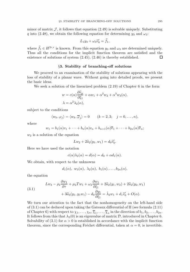
§3. STABILITY OF BRANCHING-OFF SOLUTIONS 295
minor of matrix J , it follows that equation (2.49) is solvable uniquely. Substitutingq into (2.48), we obtain the following equation for determining y3 and ω3:
L1y3 + ω3v′0 = f1,
where f1 ∈H2r,r is known. From this equation y3 and ω3 are determined uniquely.Thus all the conditions for the implicit function theorem are satisfied and theexistence of solutions of system (2.45), (2.46) is thereby established.
§3. Stability of branching-off solutions
We proceed to an examination of the stability of solutions appearing with theloss of stability of a planar wave. Without going into detailed proofs, we presentthe basic ideas.
We seek a solution of the linearized problem (2.19) of Chapter 6 in the form
w = c(α)∂vµ∂ξ1
+ αw1 + α2w2 + α3w3(α),
λ = α2λ2(α),
subject to the conditions
〈wk, ϕj〉 = 〈wk, ϕj〉 = 0 (k = 2, 3; j = 0, . . . , n),
wherew1 = b1(α)v1 + · · ·+ bn(α)vn + bn+1(α)v1 + · · ·+ b2n(α)vn;
w2 is a solution of the equation
Lw2 + 2a2(y1, w1) = d0v′0.
Here we have used the notation
c(α)λ2(α) = d(α) = d0 + αd1(α).
We obtain, with respect to the unknowns
d1(α), w3(α), λ2(α), b1(α), . . . , b2n(α),
the equation
(3.1)Lw3 − ρ2
∂w1
∂τ+ µ2Tw1 + ω2
∂w1
∂ξ1+ 2a2(y1, w2) + 2a2(y2, w1)
+ 3a3(y1, y1w1)− d0∂y1∂ξ1
= λ2w1 + d1v′0 +O(α).
We turn our attention to the fact that the nonhomogeneity on the left-hand sideof (3.1) can be deduced upon taking the Gateaux differential of Π (see formula (2.11)of Chapter 6) with respect to χ1, . . . , χn, χ1, . . . , χn in the direction of b1, b2, . . . , b2n.It follows from this that λ2(0) is an eigenvalue of matrix D, introduced in Chapter 6.Solvability of (3.1) for α > 0 is established in accordance with the implicit functiontheorem, since the corresponding Frechet differential, taken at α = 0, is invertible.
Part III
Waves in Chemical Kineticsand Combustion
CHAPTER 8
Waves in Chemical Kinetics
§1. Equations of chemical kinetics
1.1. Nondistributed system. We consider a system of n reactions
(1.1)m∑k=1
αikAk →m∑k=1
βikAk (i = 1, . . . , n).
Here Ak (k = 1, . . . ,m) denote substances taking part in the reactions; αik, βikare nonnegative integers, the stoichiometric coefficients. In order to minimize thenotation, we denote concentrations of the substances by the same letters. If noaccount is taken of spatial distributions of concentrations and it is assumed thatreactions take place at constant volume, then the change in concentrations withtime is described by the following system of equations (see, for example, [Ema 1]):
(1.2)dAkdt
=n∑i=1
γikwi (k = 1, . . . ,m),
where wi is the rate of the ith reaction, and γik = βik − αik. We shall assume thatthe rates wi may be expressed in terms of the concentrations in the following way:
(1.3) wi = Ki(T )Aνi11 × · · · ×Aνi1
m gi(A).
Here A = (A1, . . . , Am) is the vector of concentrations; νik are arbitrary realnumbers such that νik 1 if αik = 0, and νik = 0 if αik = 0; gi(A) > 0if Ak 0 (k = 1, . . . ,m); the functions Ki(T ) 0 describe the temperaturedependence of the reaction rate. Expression (1.3) encompasses the most frequentlyencountered forms for the dependence of rate on concentrations. In particular,νik = αik, gi(A) = 1 corresponds to the law of mass action.
In the case of a nonisothermal process, there must be adjoined to the sys-tem (1.2) an equation describing the variation of temperature with time. It has theform
(1.4)dT
dt=
n∑i=1
qiwi,
where qi denotes thermal effect of the reactions, which we assume to be constant.
299
300 8. WAVES IN CHEMICAL KINETICS
It is convenient to write system (1.2) in matrix form:
(1.5)dA
dt= Γw,
where, as above, A is the vector of concentrations, w = (w1, . . . , wn) is the vectorof reaction rates, and
(1.6) Γ =
γ11 · · · γn1. . . . . . . . . . .γ1m · · · γnm
is the matrix of stoichiometric coefficients. In system (1.5) vectors A and w aretreated as columns, while Γw is to be understood as the product of Γ by columnw.
Let the rank of matrix Γ be r. Then for m> r there are linear relations amongthe rows of matrix Γ:
(1.7)m∑k=1
γikσk = 0 (i = 1, . . . , n).
To each solution σ1, . . . , σm of equation (1.7) there corresponds a balance of mass:
(1.8)m∑k=1
σkAk(t) = const .
This follows directly from (1.2) if we multiply the equations by σk and add.System (1.7) has m − r linearly independent solutions. We denote them by σlk(k = 1, . . . ,m; l = 1, . . . ,m− r). To each such solution there corresponds a plane
(1.9)m∑k=1
σlkAk = al (l = 1, . . . ,m− r)
in the m-dimensional space Rm. It follows from the aforesaid that this plane isinvariant for system (1.2), i.e., if the initial values of Ak (for t = 0) belong to thisplane, then the solutions of system (1.2) belong to it for all t 0. Moreover, itis known (see, for example, [Vol 9]) that if the initial conditions for system (1.2)are nonnegative, which, understandably, corresponds to the physical meaning ofconcentrations, then solutions of system (1.2) are also nonnegative. It is thereforenatural to consider only nonnegative solutions of system (1.2). It follows, fromwhat has been said, that the polyhedron Π in space Rm defined by equations (1.9)and inequalities Ak 0 (k = 1, . . . ,m) is invariant for system (1.2) in the senseindicated above: if the initial conditions belong to polyhedron Π, then solutions ofthe system will belong to this polyhedron for all t 0. We shall refer to polyhedronΠ as the balance polyhedron. Numbers al appearing in (1.9) are determined, as arule, by assigning initial conditions for system (1.2), or (as will be seen from whatfollows) by assigning boundary conditions in the case of a spatial distribution forthe system. In the case m = r the balance polyhedron coincides with the octantAk 0 (k = 1, . . . ,m).
§1. EQUATIONS OF CHEMICAL KINETICS 301
It is convenient to specify polyhedron Π parametrically in the form
(1.10) Ak =r∑i=1
pikui +A0k (k = 1, . . . ,m),
where the point u = (u1, . . . , ur) ranges over some polyhedron of space Rr, andA0 = (A0
1, . . . , A0m) is a given fixed point belonging to Π. We write (1.10) in matrix
form:
(1.11) A = Pu+ A0,
where
P =
p11 · · · pr1. . . . . . . . . .p1m · · · prm
.Matrix P , with whose aid a parametric representation of polyhedron Π is specified,can be chosen in various ways. Selection of this matrix turns out to be importantfor the sequel, since, by means of the substitution (1.11), the system (1.2) andthe corresponding system in the spatially distributed case reduce to a new systemof equations possessing certain properties (for example, positiveness of the source,monotonicity). Therefore, we describe the general form of matrix P , which is easyto do. Indeed, let σl = (σl1, . . . , σ
lm) be the solution vector for system (1.9). Since
A − A0 is orthogonal to σl, then, obviously, the columns of matrix P must beorthogonal to σl (l = 1, . . . ,m − r), i.e., the columns of matrix P form a basisof subspace Rr0 of space Rm, orthogonal to vectors σl (l = 1, . . . ,m − r). On theother hand, it follows from (1.7) that the columns of matrix Γ belong to Rr0 and,since the rank of matrix Γ is equal to r, the columns of matrix P are then linearcombinations of the columns of matrix Γ. Thus, for P we can take an arbitrarymatrix whose columns are linearly independent and are linear combinations of thecolumns of matrix Γ.
A simpler, but rather important, special case is the case in which r = n. Thismeans that the columns of matrix Γ are linearly independent. In this case we saythat the reactions (1.1) are linearly independent, since the functions
(1.12) γi(A) =m∑k=1
βikAk −m∑k=1
αikAk =m∑k=1
γikAk (i = 1, . . . , n)
are linearly independent. For linearly independent reactions, for P we can take thematrix Γ.
We consider now equation (1.4) for the temperature. Let q = (q1, . . . , qn) bethe vector of thermal effects of the reactions. We assume that a vector τ existssuch that
(1.13) τΓ = q.
This agrees with known physical representations concerning nonisothermal reac-tions. From (1.4) and (1.5) it follows that
(1.14) T (t)− τA(t) = const .
We can describe an invariant set, including the temperature T , by adjoining
302 8. WAVES IN CHEMICAL KINETICS
to (1.11) the equation
(1.15) T = τPu + T 0.
Thus we obtain an invariant polyhedron in (m + 1)-dimensional space of concen-trations A and temperature T . We denote this polyhedron by Π.
We now present a class of chemical reactions (1.1) of importance for the sequel.Following the terminology introduced earlier, we speak of a system of reactions (1.1)as reactions with an open graph if there exists a vector s such that
(1.16) sΓ < 0.
Let s = (s1, . . . , sm). Relation (1.16) then can be written asm∑k=1
αiksk >m∑k=1
βiksk (i = 1, . . . , n).
It is easy to see that reactions with an open graph cannot contain reversiblestages. However, they form a very broad class of irreversible reactions encompassingthe majority of irreversible reactions arising naturally in chemical kinetics. To thisclass, in particular, belong all linearly independent reactions since in this case thesystem of equations sΓ=−µ, with positive vector µ, is solvable. By virtue of (1.13),the class in question also includes reactions with positive thermal effects.
We consider the stationary points of the kinetic system (1.5) in the case ofreactions with an open graph. It follows directly from (1.5) and (1.6) that at thestationary points
(1.17) wi = 0 (i = 1, . . . , n).
This means, based on (1.3), that at stationary points some concentrations vanish,i.e., all the stationary points are located on the boundary of the balance polyhedron.
We introduce the function
(1.18) V (A) = (s,A),
where, as usual, (s,A) denotes the scalar product of vectors. This function isa Lyapunov function for system (1.5) since, on the basis of (1.16), its derivativewith respect to t is, by virtue of system (1.5), negative along the trajectories ofsystem (1.5) outside of the stationary points and vanishes at the stationary points.
We shall assume that function V (A) is bounded from below on the polyhedronΠ. This is natural for chemical kinetics and holds, for example, if s 0 orpolyhedron Π is bounded.
It follows from the boundedness from below of function V (A) on Π that thisfunction attains its smallest value on Π, which we denote by Vmin. The smallestvalue may be attained at more than one point. Let Π+ be the set of those A ∈ Πfor which
(1.19) V (A) = Vmin.
It is clear, from the linearity of function V (A), that Π+ is a face of the polyhedronΠ. Moreover, all points A ∈ Π+ are stationary points of system (1.5). Toeach concentration A+ ∈ Π+ there corresponds a temperature T+, which canbe calculated from (1.15) if for u we substitute u+ corresponding to A+. Thuswe obtain a set of stationary points A+, T+ of the kinetic system (1.5), (1.4),
§1. EQUATIONS OF CHEMICAL KINETICS 303
which we denote by Π+. The set Π+ is an asymptotically stable stationary set forsystem (1.5), (1.4) in Π. This follows directly from the properties of function V (A).
In the invariant polyhedron Π there can also be other stationary points ofsystem (1.5), (1.4), i.e., stationary points A, T , at which V (A) > Vmin. Assumethat A, T is isolated in Π. We show that it is unstable. Indeed, let us join Awith A+ by a rectilinear segment. Function V (A) is linear and is therefore strictlydecreasing from A to A+. Thus, taking point A0 arbitrarily close to A and lyingon the indicated segment, we find that V (A0) < V (A) and, consequently, thetrajectory, starting at A0, will “depart” from A since along it V (A) is decreasing.Similarly, we can show that an isolated stationary face Π not intersecting Π+ is alsounstable: there exists a neighborhood of face Π in Π such that trajectories startingfrom certain points of this neighborhood, arbitrarily close to Π, depart from thisneighborhood and do not return to it.
We illustrate the above with an example, which is of independent interest asthe model of a cold flame. We shall return to this example again in §3, where, as aconsequence of general results, the existence and stability of a cold flame, describedby this model, will be proved. We consider the following three stages of a generalscheme for the oxidation reaction of carbon bisulfide (see [Kon 1, Nov 3, Zel 5]):
O + CS2 −→ COS + S,
S +O2 −→ SO +O,
SO + SO −→ SO2 + S.
We denote CS2, O, S, O2, SO, by A1, A2, A3, A4, A5, respectively (SO2 and COSneed not be taken into account). In this notation the scheme for the reactions maybe written in the form
(1.20) A1 +A2 −→ A3, A3 +A4 −→ A2 +A5, 2A5 −→ A3.
System (1.2), in the given case, has the form
(1.21)A1 = w1, A2 = w1 + w2, A3 = w1 − w2 + w3,
A4 = −w2, A5 = w2 − 2w3,
where overdots indicate differentiation with respect to t. The rates wi, by the lawof mass action, may be expressed in terms of the concentration as follows:
(1.22) w1 = K1A1A2, w2 = K2A3A4, w3 = K3A25.
The reactions are assumed to be isothermal and, therefore, we do not consider anequation for the temperature T , and we regard the reaction rate constants to beindependent of T .
We determine the vectors σ, needed to construct the balance polyhedron. Wenote that in writing equation (1.7) it is sufficient to replace Ak in the scheme of
304 8. WAVES IN CHEMICAL KINETICS
reactions by σk and the arrows by equal signs. For the reaction scheme (1.20),therefore, we obtain
σ1 + σ2 = σ3, σ3 + σ4 = σ2 + σ5, 2σ5 = σ3.
This system has two linearly independent solutions: σ(1) = (1, 1, 2, 0, 1) and σ(2) =(0, 2, 2, 1, 1). Thus the balance polyhedron Π is given by the relations
(1.23) A1 +A2 + 2A3 + A5 = a1, 2A2 + 2A3 +A4 +A5 = a2,
Ak 0 (k = 1, . . . , 5), where a1 > 0, a2 > 0. In order to find the stationary points ofsystem (1.21), it is necessary to equate the rates (1.22) to zero and to take solutionslying in the balance polyhedron (1.23):
(1.24) A1A2 = 0, A3A4 = 0, A5 = 0.
We shall not enumerate all the possibilities existing here, but limit the discussionto the case in which A4 > 0 at a stationary point. This assumption has acompletely clear physical meaning: for the oxidation reaction of carbon bisulfideCS2 considered here, it is assumed that oxygen O2 is available in abundance andcannot be all used up. Thus we have the following stationary points:
A(1) = (0, a1, 0, a2 − 2a1, 0), A(2) = (a1, 0, 0, a2, 0),
where it is assumed that a2 > 2a1. Obviously, reactions (1.20) are reactions withan open graph and as V (A) we can take the function
V = A1 +A2 +A3 + 2A4 +A5,
so that the derivative along the trajectories of system (2.1) is equal to
V = −(w1 + w2 + w3).
Since V (A(1)) = 2a2 − 3a1 < V (A(2)) = 2a2 + a1, it follows that A(1) is an asymp-totically stable point in Π, and A(2) is unstable. We can give this result concerningexistence and stability of stationary points the following physical interpretation. Atpoint A(1) the concentration of the initial substance A1 = CS2 is equal to zero, i.e.,the substance is completely used up and the reaction can no longer continue. It isclear that with a small change of concentrations the system reverts to the same stateindicating asymptotic stability of a stationary point. The second stationary pointA(2) is of an entirely different nature. At this point concentrations of the activecenters A2 = O and A3 = S are equal to zero, and, as is evident from the reactionscheme (1.20), the reaction cannot proceed. Small perturbations, i.e., the additionof a small amount to at least one of the active centers, lead to a development ofthe reaction since active centers will be formed later in the process of the reaction,and the reaction will continue so long as the initial substance CS2 is not used up,i.e., the system arrives at the stationary state indicated above.
1.2. Waves. In the case of a spatially nonhomogeneous system it is necessaryto take into account the distribution of concentrations and temperature over space,
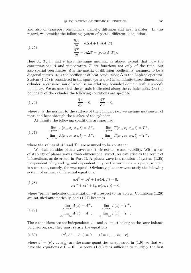
§1. EQUATIONS OF CHEMICAL KINETICS 305
and also of transport phenomena, namely, diffusion and heat transfer. In thisregard, we consider the following system of partial differential equations:
(1.25)
∂A
∂t= d∆A + Γw(A, T ),
∂T
∂t= κ∆T + (q, w(A, T )).
Here A, T , Γ, and q have the same meaning as above, except that now theconcentrations A and temperature T are functions not only of the time, butalso spatial coordinates; d is the matrix of diffusion coefficients, assumed to be adiagonal matrix; κ is the coefficient of heat conduction; ∆ is the Laplace operator.System (1.25) is considered in the space (x1, x2, x3) in an infinite three-dimensionalcylinder, a cross-section of which is an arbitrary bounded domain with a smoothboundary. We assume that the x1-axis is directed along the cylinder axis. On theboundary of the cylinder the following conditions are specified:
(1.26)∂A
∂ν= 0,
∂T
∂ν= 0,
where ν is the normal to the surface of the cylinder, i.e., we assume no transfer ofmass and heat through the surface of the cylinder.
At infinity the following conditions are specified:
(1.27)limx1→∞
A(x1, x2, x3, t) = A+, limx1→∞
T (x1, x2, x3, t) = T+,
limx1→−∞
A(x1, x2, x3, t) = A−, limx1→−∞
T (x1, x2, x3, t) = T−,
where the values of A± and T± are assumed to be constant.We shall consider planar waves and their existence and stability. With a loss
of stability of planar waves, three-dimensional structures can arise as the result ofbifurcations, as described in Part II. A planar wave is a solution of system (1.25)independent of x2 and x3, and dependent only on the variable x = x1 − ct, where cis a constant, namely, the wavespeed. Obviously, planar waves satisfy the followingsystem of ordinary differential equations:
(1.28)dA′′ + cA′ + Γw(A, T ) = 0,
κT ′′ + cT ′ + (q, w(A, T )) = 0,
where “prime” indicates differentiation with respect to variable x. Conditions (1.26)are satisfied automatically, and (1.27) becomes
(1.29)limx1→∞
A(x) = A+, limx1→∞
T (x) = T+,
limx1→−∞
A(x) = A−, limx1→−∞
T (x) = T−.
These conditions are not independent: A+ and A− must belong to the same balancepolyhedron, i.e., they must satisfy the equations
(1.30) (σl, A+ − A−) = 0 (l = 1, . . . ,m− r),
where σl = (σl1, . . . , σlm) are the same quantities as appeared in (1.9), so that we
have the equations σlΓ = 0. To prove (1.30) it is sufficient to multiply the first
306 8. WAVES IN CHEMICAL KINETICS
equation in (1.28) by σl and integrate along the axis. As was the case in (1.13), weobtain
(1.31) T+ − T− = (τ, A+ −A−).
Thus for a wave to exist it is necessary that conditions (1.30), (1.31) be satisfied. Weshall assume that these conditions are satisfied. As is usual, we assume that pointsA+, T+ and A−, T− are stationary points of the corresponding nondistributedsystem (1.5), (1.4), i.e.,
Γw(A+, T+) = 0, (q, w(A+, T+)) = 0,(1.32)
Γw(A−, T−) = 0, (q, w(A−, T−)) = 0.(1.33)
We assume also that the point A−, T− belongs to an asymptotically stable (closed)stationary face Π− of the balance polyhedron Π. In particular, this can be anisolated asymptotically stable stationary point.
The second stationary point A+, T+ can be of a different nature. We shallconsider two cases, which we can refer to as the stationary state of thermal andkinetic nature. The first of these cases is realized for reactions with a strongdependence of the reaction rate on the temperature. At low temperature thereactions take place so slowly that, to a fairly good approximation, their ratescan be assumed equal to zero:
(1.34)Ki(T ) = 0 for T T ∗,
Ki(T ) > 0 for T > T ∗,i = 1, . . . , n,
where T ∗ is a number between T− and T+. Such an approach, namely, oneinvolving a source cut-off, is typical for problems of combustion (see [Zel 5]). It isclear, by virtue of (1.3), that all the rates wi(A+, T+) are equal to zero and thatequations (1.33) are valid.
In the second of the cases considered the source cut-off is not made and thestationary point is of a kinetic character. Typical examples for this case includecold flame, the Belousov-Zhabotinsky reaction, and a number of nonisothermalchain reaction processes with a weak temperature dependence of the reaction rate.Here the stationary point A+, T+ belongs to a (closed) stationary face Π+ of thepolyhedron Π, which can be both stable as well as unstable. In what follows, weshall assume that Π+ and Π− have no points in common.
As an example, we can consider the case of reactions with on open graph. HereΠ− can be defined as the face of balance polyhedron Π on which V (A) attains aminimum. As was indicated above, this is an asymptotically stable stationary face.The second stationary face Π+, if it exists and is isolated, is unstable. In the coldflame model of (1.20) presented above, there are low isolated stationary points:asymptotically stable and unstable. We present other examples below.
§2. Monotone systems
In this section we study wave solutions of kinetic systems which, by means of alinear change of variables of the form (1.11), can be reduced to monotone systems,considered in Chapters 3 and 5. The existence and stability of waves for systems ofchemical kinetics will follow from results obtained in this chapter. Various kineticsystems encountered in applications will be considered.
§2. MONOTONE SYSTEMS 307
2.1. Reduction to monotone systems. We consider the kinetic system(1.2) and in it make the substitution (1.11). For definiteness, we shall assumethat the first r reactions in system (1.1) are linearly independent, which results inno loss of generality since the reactions can be renumbered. This means that thefirst r columns of matrix Γ (see (1.6)) are linearly independent. As the matrix Pwe can take the matrix consisting of the first r columns of matrix Γ. Then the newvariables ui (i = 1, . . . , r) are introduced by the equations
(2.1) Aj =r∑i=1
γijui +A+j (j = 1, . . . ,m),
where the boundary condition is taken as the fixed point A+. Since all the columnsof matrix Γ, beginning with the (r + 1)st, depend linearly on the first r columns,we then have the equations
(2.2) γkj =r∑i=1
λkiγij (k = r + 1, . . . , n),
where λki are certain numbers. Substituting these expressions into the system ofequations (1.2), we obtain
(2.3)dAjdt
=r∑i=1
γij
(wi +
n∑k=r+1
λkiwk
)(j = 1, . . . ,m).
We can now go over to the new variables uj in accordance with formulas (2.1):
r∑i=1
γijduidt
=r∑i=1
γij
(wi +
n∑k=r+1
λkiwk
)(j = 1, . . . ,m).
Taking into account that the rank of matrix Γ is equal to r, it follows that
(2.4)duidt
= wi +n∑
k=r+1
λkiwk (i = 1, . . . , r).
This system of equations is equivalent to system (1.2). It is assumed here that inequation (1.3) the reaction rate Aj has been replaced by its expression from (2.1).In the nonisothermal case it is necessary to substitute the temperature into theexpression (1.3) for the rates using equation (1.15). Recalling that as the matrix Pwe have taken the first r columns of matrix Γ, we have, taking into account (1.13),
(2.5) T =r∑i=1
qiui + T+.
After making the indicated substitutions, we denote the right-hand side of (2.4) byFi(u):
(2.6) Fi(u) = wi +n∑
k=r+1
λkiwk (i = 1, . . . , r).
By definition (see Chapter 3), the condition for monotonicity of the system amounts
308 8. WAVES IN CHEMICAL KINETICS
to the validity of the following inequalities:
(2.7)∂Fi(u)∂uj
0 (i, j = 1, . . . , r; i = j).
We need to obtain these conditions in explicit form using (1.3), whereby throughoutthis section we assume that gi(A) = 1 and that
(2.8) K ′i(T ) 0 (i = 1, . . . , n).
We remark that this latter condition is satisfied, in particular, for the Arrheniustemperature dependence of the reaction rate,
(2.9) Ki(T ) = K0i e
−Ei/RT ,
where K0i , Ei, and R are constants; Ei is the activation energy; R is the universal
gas constant.A direct calculation yields
(2.10)∂wi∂uj
= wi
[ m∑k=1
νikγjkAj
+K ′i(T )
Ki(T )qj
].
In particular, in the case of Arrhenius temperature dependence,
(2.11)∂wi∂uj
= wi
[ m∑k=1
νikγjkAj
+EiRT 2
qj
].
We return now to system (2.4). We begin with the case in which reactions (1.1)are linearly independent (r = n). System (2.4) then has the form
(2.12)duidt
= wi (i = 1, . . . , n)
and sufficient conditions for its monotonicity can be written, by virtue of (2.10), inthe following way:
(2.13) νikγjk 0, qj 0 (i, j = 1, . . . , n; k = 1, . . . ,m; i = j).
These conditions are considered in greater detail in the following section.We pass over now to the general case of system (2.4). From (2.6) and (2.10)
we obtain
(2.14)∂Fi∂uj
= wi
[ m∑k=1
νikγjkAk
+K ′i(T )
Ki(T )qj
]+
n∑l=r+1
λliwl
[ m∑k=1
νlkγjkAk
+K ′i(T )
Ki(T )qj
].
Sufficient conditions for monotonicity take the form
(2.15) νikγjk 0, λliνlkγjk 0, qj 0, λliqj 0
for all i, j = 1, . . . , r, i = j; l = r + 1, . . . , n; k = 1, . . . ,m.Conditions described in this form are inconvenient for application. In the
following section we supply a simpler interpretation for them.
§2. MONOTONE SYSTEMS 309
2.2. Monotonicity conditions. To obtain a form of the monotonicity con-ditions (2.15), more suitable for application, we consider the linear forms γi,corresponding to reactions (see (1.12)), and νi (corresponding to rates (see (1.3)):
γi(A) = γi1A1 + · · ·+ γimAm (i = 1, . . . , n)(2.16)
νi(A) = νi1A1 + · · ·+ νimAm.(2.17)
Only signs of the coefficients of the Ak are of interest to us here. Therefore, insteadof (2.17), we can consider the form
(2.18) αi(A) = αi1A1 + · · ·+ αimAm,
connected with the left-hand sides of reactions (1.1). Such an approach to forms ismore suitable since many of the coefficients αij , γij are equal to zero. For example,for the reactions (1.20), we have
(2.19)α1 = A1 +A2, α2 = A3 +A4, α3 = 2A5,
γ1 = A3 −A1 −A2, γ2 = A2 +A5 −A3 −A4, γ3 = A3 − 2A5.
We begin with the isothermal case, i.e., we assume that qi = 0 (i = 1, . . . , n).First let us give an interpretation of the first of inequalities (2.15). We compare
forms αi(A) with γj(A) (i = j). We say that an element Ak is an element commonto these forms if it appears in both of these forms with nonzero coefficients. Forexample, in (2.19) α1 and γ2 have the common element A2; α1 and γ3 have noelements in common.
The first of the conditions (2.15) consists in the following.
Condition 1. In the forms αi and γj (i, j = 1, . . . , r; i = j), all elements incommon, if they exist, must be of the same sign.
It is readily verified that this condition is satisfied for the forms (2.19). We notethat the forms α1 and γ1 have elements A1 and A2 in common, but with oppositesigns; however, they must not be compared since the comparison is to be made fori = j.
We consider yet another example, also of interest, since it represents a modelof a heterogeneous catalytic reaction for which the condition for existence andstability of an isothermal wave is satisfied (see §3). This model was studied byV. I. Bykov [Byk 1] from the point of view of a multiplicity of stationary states ofa nondistributed system. The scheme of the reactions has the form
(2.20) kA1 ↔ kA2, lA2 ↔ lA3, pA1 + qA3 → (p+ q)A2,
where k, l, p, and q are positive integers.Taking into account reverse reactions, we find that this scheme contains five
reactions, which we renumber so that the first three reactions will be direct. Inaccordance with this, we have
α1 = kA1, α2 = lA2, α3 = pA1 + qA3, α4 = kA2, α5 = lA3,
γ1 = k(A2 −A1), γ2 = l(A3 −A2), γ3 = (p+ q)A2 − pA1 − qA3,
γ4 = k(A1 −A2), γ5 = l(A2 −A3).
310 8. WAVES IN CHEMICAL KINETICS
The first two reactions are linearly independent; the remaining ones depend onthem linearly:
(2.21) γ3 =p
kγ1 −
q
lγ2, γ4 = −γ1, γ5 = −γ2.
Verification of the first of inequalities (2.15) consists in comparing α1 with γ2 andα2 with γ1. The condition is obviously satisfied.
Consider now the second of inequalities (2.15). The numbers λli appearing hereexpress, by virtue of (2.2), the linear dependence of the forms γi:
(2.22) γl =r∑i=1
λliγi (l = r + 1, . . . , n).
It is convenient to introduce the formiαl = sgnλli · αl
and take no account of zero forms. The second of the conditions (2.15) is thenformulated in a manner completely similar to the first.
Condition 2. In formsiαl and γj (i, j = 1, . . . , r; i = j; l = r + 1, . . . , n) all
common elements, if any, must be of the same sign.
For example, for reactions (2.20) we have the forms1α3 = α3,
1α4 = −α4. These
must be compared with γ2. Next,2α3 = −α3,
2α5 = −α5 are compared with γ1.
We see that common elements, where they are present, appear with identical signs.Consequently, the monotonicity conditions are satisfied for reactions (2.20).
We point out two classes of reactions for which the conditions of monotonicitycan be formulated most simply. The first of these is the class of linearly independentreactions. In this case, it is obviously necessary to verify only Condition 1. It isclear that if each substance Ak is consumed (i.e., is found on the left side) in no morethan a single reaction, Condition 1 is satisfied. In other words, a sufficient conditionfor monotonicity for linearly independent reactions is the absence of parallel stages.Thus, for example, reactions (1.20) are linearly independent and in them there areno parallel stages.
The second class of reactions we consider are reversible reactions in which thedirect reactions are linearly independent. It is convenient to introduce, along withαi and γi, the additional form
βi(A) = βi1A1 + · · ·+ βimAmand to write reactions in the following form:
αi(A)→ βi(A) (i = 1, . . . , r),(2.23)
βi(A)→ αi(A) (i = 1, . . . , s),(2.24)
where s r. Condition 1 must be satisfied for the reactions (2.23); Condition 2must be satisfied for reactions (2.24). In order to make the notation consistentwith that introduced earlier, we set αi+r = βi (i = 1, . . . , s), γi+r = −γi. From
this we haveiαi+r = −βi. Condition 2 now looks as follows: in the forms −βi
and γj (i = 1, . . . , s; j = 1, . . . , r) common elements, if they are present, mustappear with identical signs. Thus we can state the following sufficient condition
§2. MONOTONE SYSTEMS 311
for monotonicity for the reactions (2.23), (2.24): reactions (2.23) must not haveparallel stages; the substances that appear on the left side of the ith reactionof (2.24) (i = 1, . . . , s) must not appear in βj (j = 1, . . . , r; i = j). In particular,when r = s, reversible reactions must not have parallel stages. For example, inreactions (1.20) we can include a reverse stage for the second reaction withoutviolation monotonicity conditions, but this cannot be done for the first reaction.
Remark. In the case of linearly independent reactions the requirement thatparallel stages be absent is sufficient for Condition 1 to be satisfied, but it is notnecessary. It is equivalent to Condition 1 only when the substances on the rightand left sides of the reactions are completely different. In the contrary case, we canallow the presence of parallel stages. For example, for a system of auto-catalyticreactions
A1 +A2 −→ 2A1 + · · · , A1 +A3 −→ A1 + · · · ,
Condition 1 is satisfied.
We have considered the isothermal case. For nonisothermal processes additionalconditions on thermal effects of the reactions are appended. If the reactions arelinearly independent, it follows from (2.13) that, in addition to Condition 1, it issufficient to require that the thermal effects be nonnegative.
In the general case, presence of the condition λliqj 0 can imply that certainthermal effects must be equal to zero. However, this result can be connected onlywith the method of reduction to monotone systems. We turn our attention to thisin greater detail.
All the conditions for reducibility to monotone systems, formulated in thissection, were obtained on the assumption that, as the matrix P appearing in (1.11),the first r columns of matrix Γ were used. However, a choice of this kind for matrixP is not mandatory. As a consequence of what was said in §1,
(2.25) P = ΓM,
where as M we can take an arbitrary m× n matrix such that P is of rank r. Thechoice of matrixM can be important for the possibility of a reduction to monotonesystems: as is easily seen from examples, the choice of linearly independent columnsof matrix Γ, that are taken as P , is also important. Therefore, the class of systems,reducible to monotone systems, can be broadened by including matrix M in themonotonicity condition and then selecting it. It will be shown in the followingchapter that for reactions with an open graph, and not only for linearly independentreactions, the matrix P can be chosen so that the resulting monotonicity conditionsare satisfied for arbitrary nonnegative thermal effects.
We show now how the reduction to a monotone system using (2.25) may becarried out. From (1.11) and (1.5) we have
Pdu
dt= Γw.
Let N be an r × n matrix such that
(2.26) Γ = PN.
It is obvious that matrix N may be determined uniquely. Thus
(2.27)du
dt= F (u),
312 8. WAVES IN CHEMICAL KINETICS
where
(2.28) F (u) = Nw(Pu+A+, τPu + T+).
It is easy to see that system (2.27) is equivalent to (1.5), (1.4). We requirematrix (2.28) to satisfy condition (2.7).
One of the possibilities for realizing such an approach consists in adjoining tothe given system of reactions (1.1) new reactions that are linear combinations of thegiven reactions, selecting linearly independent reactions in the broadened systemof reactions, and verifying Conditions 1 and 2. In the system (2.27), so obtained,rates corresponding to the introduced reactions are discarded.
As an example, we consider the system of reactions
(2.29) 2A1 −→ 2A2, A1 −→ A3, A2 +A3 −→ 2A1.
The first two reactions are linearly independent. The third one linearly depends onthem. The first two reactions contain parallel stages and do not satisfy Condition 1.To this system we adjoin the reaction A3→A1 and we select it and the first reactionas linearly independent reactions in terms of which the rest are expressed. It isreadily verified that Conditions 1 and 2 are satisfied.
§3. Existence and stability of waves
In this section we prove existence and stability of waves for kinetic systemsreducible to monotone systems. As a preliminary, for a system of equations (1.28)describing traveling waves, assuming equality of transport coefficients, we performthe same kind of reduction to monotone systems that was done in the precedingsection for a nondisturbed system.
3.1. Passage to new variables. From the dependent variables A and T wego over to new variables u in accordance with equations (1.11), (1.15):
(3.1) A(x) = Pu(x) +A+, T (x) = τPu(x) + T+,
where A+, T+ are specified from conditions (1.29) and matrix P is given byequation (2.25). Taking equation (2.26) into account and regarding d to be a scalarmatrix, we obtain
(3.2) P (du′′ + cu′ +Nw) = 0.
Since P has rank r, it then follows from this that
(3.3) du′′ + cu′ + F (u) = 0,
where
(3.4) F (u) = Nw(Pu+A+, τPu + T+).
Conditions for u at infinity are obtained from (1.29) and (3.1):
(3.5) limx→∞
u(x) = u+, limx→−∞
u(x) = u−,
where u+ = 0 and u− is obtained from the equations
(3.6) Pu− = A− −A+.
We note, by virtue of (1.30), that this system of equations has a solution.
§3. EXISTENCE AND STABILITY OF WAVES 313
For κ = d, it is clear, conversely, that if u(x) is a solution of problem (3.3),(3.5), then functions A(x), T (x), specified by equations (3.1), are solutions ofproblem (1.28), (1.29). Indeed, multiplying (3.3) by P , we obtain (3.2), and,consequently, A is a solution of the first of equations (1.28). Next, we multiply (3.2)scalarly by vector τ and take note of (1.13). We find that T satisfies the second ofequations (1.28). From (3.5), (3.6), and (1.31) it follows that conditions (1.29) aresatisfied.
Thus we have obtained problem (3.3), (3.5), a problem equivalent to theproblem (1.28), (1.29).
3.2. Existence and stability of waves. To prove the existence of solutionsof problem (1.28), (1.29) it would be sufficient to use Theorem 4.2 of Chapter 3 forthe monotone system (3.3). However, this cannot be done directly for the followingreason. In the proof of the theorem indicated, it was assumed that the vector-valuedfunction F (u) is given in the interval [u+, u−] and satisfies there the monotonicitycondition. In the case considered here, this, generally speaking, is not so. FunctionF (x) is given in the balance polyhedron Πu, which may not be an interval. It willtherefore be necessary for us to supplement the proof of the theorem in connectionwith this case. Actually, this means that we shall need to verify the nonnegativenessof the concentrations A(x) in the course of the proof.
We introduce the quantity ω∗, defined by equations (4.4) and (4.5) of Chapter 3.It is assumed here that K is constricted owing to the addition of the conditionPρ(x) +A+ 0, i.e., that ρ(x) ∈ Πu.
The existence theorem for waves may be stated as follows.
Theorem 3.1. In the balance polyhedron Πu let the vector-valued functionF (u), given by equation (3.4), satisfy the monotonicity condition
∂Fi(u)∂uj
0 (i, j = 1, . . . , r; i = j)
and vanish only at the points u+ and u−. Assume, further, that a vector p 0,p = 0, exists such that
(3.7) F (u+ + sp) 0 for 0 < s s0,
where s0 is a positive number. Then, assuming that u− > u+, there exists, forall c ω∗, a monotonically decreasing solution u(x) of system (3.3), satisfyingconditions (3.5), such that the functions A(x), specified by equations (3.1), arenonnegative. When c < ω∗, such solutions do not exist.
Proof. We shall not repeat in full the proof of Theorem 4.2 of Chapter 3, butshall supply only the necessary additions. We assume, first, that c > ω∗. Then,according to the definition of the number ω∗, there exists ρ(x) ∈ K, such that
(3.8) dρ′′(x) + cρ′(x) + F (ρ(x)) < 0
for all x. We consider a boundary problem for system (3.3) on the semi-axis x < bwith the condition (4.9) of Chapter 3:
(3.9) u(b) = sp+ u+.
We show that there exists a monotonically nonincreasing solution of this problem
314 8. WAVES IN CHEMICAL KINETICS
u(x) ∈ Πu. To do this, we consider the problem
(3.10)∂v
∂t= d
∂2v
∂x2+ c∂v
∂x+ F (v), t > 0, x < b,
v(b, t) = u(b), v(x, 0) = u(b).
Let
(3.11) A(x, t) = Pv(x, t) +A+, T (x, t) = τPv(x, t) + T+.
It is clear that A(x, t) is a solution of the following problem:
∂A
∂t= d
∂2A
∂x2+ c∂A
∂x+ Γw(A, T ), t > 0, x < b,(3.12)
A(b, t) = Pu(b) +A+, A(x, 0) = Pu(b) +A+.(3.13)
By assumption, u(b) defined by equation (3.9) belongs to the polyhedron Πu.Consequently, A(b, t) 0, A(x, 0) 0. It is known (see Chapter 5) that thesolution of problem (3.12), (3.13) is nonnegative. This means that solution v(x, t)of problem (3.10), for all x < b and t > 0, belongs to the balance polyhedron Πu.Since v= u(b) is a lower function for system (3.10), the solution v(x, t) of this systemis monotonically nondecreasing with respect to t. On the other hand, ρ(b) > u(b)on the basis of (4.8) of Chapter 3. If we consider function z(x, t) = ρ(x) − v(x, t),where v(x, t) is the solution of (3.12), (3.13), then, by virtue of (3.8), z will satisfythe equation
(3.14)∂z
∂t= d
∂2z
∂x2+ c∂z
∂x+B(x, t)z,
where
B(x, t) =∫ 1
0
F ′(sρ(x) + (1− s)v(x, t)) ds,
F ′ is the matrix of partial derivatives of the vector-valued function F (u). Since ρ(x)and v(x, t) belong to Πu, we have that sρ(x) + (1 − s)v(x, t) also belongs to thispolyhedron, and, therefore, B(x, t) has nonnegative off-diagonal elements. It followsfrom (3.14) that z(x, t) 0, i.e., v(x, t) ρ(x). Thus the limit of v(x, t) as t→∞exists; we denote it by u(x). It is obvious that u(x) ρ(x). Moreover, u(x) ∈ Πufor x b. It may be proved, exactly as was done in Theorem 4.2 of Chapter 3,that u(x) is a monotonically nonincreasing solution of problem (3.9), (3.10), andall further construction proceeds in the same way. This completes the proof of thetheorem.
Remarks. 1. In the theorem it was proved that the solution u(x) of prob-lem (3.3), (3.5) belongs to the balance polyhedron Πu. It may be readily verifiedthat the set Πu can be replaced by any other positively invariant set. Let usformulate this more precisely. We first define what is meant in the present case bypositive invariance. We say that a set G ⊂ R2 is positively invariant if it is closed,convex, and if the solution v(x, t) of problem (3.10) belongs to G for all x < b, t > 0,provided that the boundary and initial condition belongs to G.
In the statement of the theorem we replace Πu throughout by G. This meansthat in the definition of ω∗ we assume that the class K is the class of monotonicallydecreasing functions ρ(x) ∈ C2, satisfying the conditions lim ρ(x) = u± as x→±∞and ρ(x) ∈ G for all x. The theorem can be stated in the following way. Suppose
§3. EXISTENCE AND STABILITY OF WAVES 315
F (u) satisfies the monotonicity condition in G and vanishes only at two points u+
and u−. Suppose, further, that a vector p 0, p = 0, exists such that u+ + sp ∈ Gand that (3.7) holds. Then for all c ω∗ there exists a monotonically decreasingsolution u(x) of problem (3.3), (3.5) such that u(x) ∈ G for all x. When c < ω∗,such solutions do not exist. The proof is similar to the previous proof.
Explicit algebraic conditions for positive invariance are known (see [Red 1] andreferences therein). Our interest centers on the case in which set G is obtained asthe intersection of polyhedron Πu with domains of the form s(u) 0, where s(u)are twice continuously differentiable functions satisfying a convexity condition andwhere the surface s(u) = 0 does not contain the point u−. The condition of positiveinvariance consists in the circumstance that vector F (u) is directed towards theinterior of domain G at points of these surfaces.
2. In the theorem it was assumed that the vector-valued function F (u) vanishesonly at the two points u+ and u− in the balance polyhedron Πu. In various problemsof chemical kinetics cases are encountered in which the stationary points u+ and(or) u− are not isolated points in Πu. To prove the existence of waves in this caseuse can be made of the following approach. We select a pair of stationary points ofinterest to us, u+ and u−, which we take as conditions at infinity. We construct, ifpossible, a positively invariant set G, as defined in the preceding remark, such thatG ⊂ Πu and such that only these two stationary points are contained in G. Basedon what was said in Remark 1, we obtain the existence of waves with the givenvalues u+ and u− at the infinities. Illustrations of this approach through modelproblems will be presented in §4.
3. A theorem for the existence of waves was proved in the monostable case.A similar result holds for the bistable case. To see this, we need to verify thatin the homotopy process used in the Leray-Schauder method, nonnegativenessof concentrations is preserved. We shall not do this here: detailed proofs in ananalogous case are provided in the following chapter (for problems of combustion).
We proceed now to the problem concerning stability of waves. We can use theresults from §4 of Chapter 5 concerning stability of waves for monotone systems.In this connection, for systems of equations of chemical kinetics, reducible tomonotone systems, results concerning stability are obtained in the variables u,introduced in §3.1. In these variables, based on Theorem 4.1 of Chapter 5, stabilityof waves occurs (if, of course, conditions for this theorem are satisfied). We canalso state results concerning stability of waves in the initial variables, which are theconcentrations A and the temperature T . This question is also pursued in moredetail in the following chapter for combustion problems.
3.3. Remarks concerning nonmonotone systems.1 For systems of equa-tions of chemical kinetics which can be reduced to monotone systems, travelingwaves, as was shown above, exist and are stable. It can be expected that existenceof waves occurs even for a more general class of systems. Above all, this concernssystems of reactions with an open graph, which, as already mentioned, encompass avery broad class of nonreversible reactions. In the bistable case this can be provedby the Leray-Schauder method in the same way it is proved in the following chapterfor problems of combustion. We remark that in that chapter a system of equations
1 The presentation in this section is of a descriptive nature and precise statements are notsupplied.
316 8. WAVES IN CHEMICAL KINETICS
of chemical kinetics is considered for the case in which a cut-off of the source maybe done. No other characteristics of combustion problems is employed.
In the monostable case application of this method is limited, first of all, to theconstruction of a rotation of the vector field, which was carried out in Chapter 2 forthe bistable case. Nevertheless, there is every reason to assume that this homotopicinvariant can also be constructed for the monostable case. Actually, if we go overto weighted spaces, selected in an appropriate manner, the monostable case canthen be reduced to the bistable case. It is true that here there appears an explicitdependence on x in the operator, which, however, must not hinder carrying-out theconstructions of Chapter 2.
There can be no stability of waves for systems of equations not reducible tomonotone systems, not even in the simplest cases. Simple examples show that ifthe transport coefficients are distinct, it is then possible that a planar wave willlose stability and that various oscillatory modes will appear. In this connection,it is of interest to consider systems homotopic to monotone systems. We meansystems of the form (1.25) which can be obtained from the monotone systems,considered above, by a continuous change in the coefficients of diffusion (here d canalready be considered not as a number, but a matrix), thermal conductivity, and thekinetic constants. It is assumed here that the stationary points of a kinetic system,which determine the conditions at infinity, vary continuously and do not changethe nature of the stability. We assume that a change in the indicated physicalquantities takes place along a curve, described with the aid of some parameter τ , sothat for τ = 0 the system is monotone. For τ = 0, a planar wave is stable, and theeigenvalues of the operator, obtained by linearization of the right-hand side of (1.25)about a planar wave, lie in the left half-plane. This was proved above in the one-dimensional case. Similarly, this may also be proved for the multi-dimensional caseupon expanding with respect to the eigenfunctions of the Laplace operator for thetransverse variables.
We shall keep track of a planar wave for motion with respect to parameter τ ,remaining within the scope of systems for which existence of a wave is known (forexample, where a priori estimates are available and the Leray-Schauder method canbe applied). For motion with respect to a parameter, the eigenvalue with maximumreal part can land on the imaginary axis and intersect it. Bifurcations, describedin Part II, will then take place.
§4. Branching chain reactions
As previously mentioned, the propagation of waves in chemical kinetics canhave not only a thermal nature, as, for example, waves of combustion, but also akinetic character. One of the most interesting classes of reactions for which suchwaves are possible is the class of branching chain reactions. In this section weconsider conditions for the existence and stability of branching chain flames, bothisothermal as well as nonisothermal.
4.1. Branching chain processes with kinetics of a general form. Weconsider the system of reactions (1.1). We divide all substances Ak (k = 1, . . . ,m)taking part in these reactions into two groups. In the first group are the initialsubstances, which we denote by A1, . . . , As (s < m). These are substances whichappear on the left sides of reactions and do not appear on the right sides; they aresubstances which are only used up but not produced. In the second group are the
§4. BRANCHING CHAIN REACTIONS 317
intermediate substances, which we denote by R1, . . . , Rp, so that As+j = Rj (j =1, . . . , p; s + p = m). In the reaction process these substances are consumed andproduced, i.e., they appear on both the left and right sides of reactions. Finalproducts, i.e., substances appearing only on the right sides of reactions, may notbe taken into account in our discussions.
We say that a system of reactions (1.1) describes a branching chain processif there exist nonnegative numbers λ1, . . . , λp such that the linear combination ofconcentrations
(4.1) U(R) =p∑j=1
λjRj
increases with respect to the time during the reaction process.It is obvious that among the numbers λj there must be positive numbers
(otherwise the sum (4.1) could not increase). Substances Rj that appear withnonzero coefficients λj are called active centers, due to which branching of a chainproceeds.
By the increase of U(R) with time during the reaction process we mean that
(4.2)dU
dt=
p∑j=1
λjdRjdt
=p∑j=1
λj
n∑i=1
γi,j+swi 0,
but not identically equal to zero. Here we have used equation (1.2) for theintermediate substances:
(4.3)dRjdt
=n∑i=1
γi,j+swi.
Obviously, the following inequality is a sufficient condition for the satisfaction ofinequality (4.2):
(4.4)p∑j=1
λjγi,j+s 0 (i = 1, . . . , n);
here at least one of these inequalities is strict. This condition can also be writtenin the matrix form
(4.5) λΓ 0,
where λ = (λ1, . . . , λp); Γ is the matrix formed from the last p rows of matrix Γ.Inequalities (4.4) have the following physical interpretation: the number of
active centers is maintained over a part of the reactions (1.1) (such reactions arecalled chain continuation reactions), but over the remaining part of the reactionsit increases (such reactions are called branching reactions).
Since our concern is the study of waves joining various stationary points ofa kinetic system, we shall be interested in the question concerning conditions fornonuniqueness of stationary points and their stability. Before formulating theseconditions, we recall that linear dependence or independence of substances is to beunderstood as linear dependence or independence of the rows of matrix Γ.
Condition 1. There exists a set of linear independent intermediate substancessuch that
318 8. WAVES IN CHEMICAL KINETICS
1) all active centers taking part in the branching of a chain are contained inthis set;
2) in each reaction at least one of these intermediate substances is used up.
In particular, this condition means that reactions initiating a chain, i.e., reac-tions on whose left sides only initial substances appear, are absent. Such reactionsare usually excluded in the study of chain flames.
Let us renumber the intermediate substances Rj so that the set in Condition 1consists of the substances R1, . . . , Rl (l p).
As in §1.1, we consider a balance polyhedron Π, which is defined by equa-tions (1.9) and inequalities Ak 0 (k = 1, . . . ,m). It is natural to considernondegenerate balance polyhedra, i.e., polyhedra containing interior points: pointsin which all concentrations Ak are positive.
Proposition 4.1. If Condition 1 is satisfied, there then exists a nondegeneratebalance polyhedron Π such that the equations
(4.6) R1 = 0, . . . , Rl = 0
specify a stationary face of this polyhedron. This face is nonattracting, i.e., semi-trajectories, departing from an arbitrary interior point of polyhedron Π, cannotstrike the face (4.6) as t→∞.
Proof. Let r be the rank of matrix Γ. Then there exist r linearly indepen-dent substances on which the remaining m − r substances depend linearly. Weselect r linearly independent substances such that all the substances R1, . . . , Rl arecontained among them; this can be done by virtue of the assumption concerningtheir linear independence. We denote all the linearly dependent substances byA1, . . . , Aq (q = m − r), and the indicated set of linearly independent substancesby Aq+1, . . . , Am. We then have equations
(4.7) Aj =r∑k=1
τjkAq+k + aj (j = 1, . . . , q),
where τjk and aj are certain numbers. To specify the balance polyhedron Π, it issufficient to prescribe the quantities aj (j = 1, . . . , q). We do this by specifyingsome point A = (A0
1, . . . , A0m) of the balance polyhedron in the following way. We
set Rj = 0 (j = 1, . . . , l). We take all the remaining independent concentrations tobe nonnegative and all the dependent ones to be positive.
It is easy to see that the balance polyhedron so constructed has interior pointsand, even more, interior points lying arbitrarily close to the face (4.6). Indeed, weconsider a point for which all concentrations, which are equal to zero at point A0,are given by small positive numbers, all remaining independent concentrations beingleft unchanged, while the dependent ones are calculated from (4.7). Moreover, theconcentrations Aj (j = 1, . . . , q) remain positive since the change in the independentconcentrations is small.
By virtue of Condition 1, face (4.6) is stationary since on it all reaction ratesvanish. It remains to show that it is nonattracting. This follows from the factthat function U(R) vanishes on face (4.6), is positive at an arbitrary interior pointof polyhedron Π, and increases along any solution. The proposition is therebyestablished.
§4. BRANCHING CHAIN REACTIONS 319
And so we see that when Condition 1 is satisfied, the balance polyhedron hasa stationary face which is nonattracting. Furthermore, in many cases there alsoexist attracting stationary faces or, in particular, asymptotically stable stationarypoints. We present two broad classes of reactions for which this situation obtains.
The first class is a class of reactions with an open graph (see §1.1). In thiscase we have the Lyapunov function (1.18). As we did above, we assume that thisfunction is bounded from below in the balance polyhedron Π. As was pointed outin §1.1, the set of points on which this function attains a minimum is asymptoticallystable.
The second class of reactions for which attracting stationary faces are possibleare those for which some part of the reactions forms reactions with an open graph,while the remaining part consists of reversible stages. In studying this class ofreactions use is made of the well-known fact (see, for example, [Vol 9]) that forreversible reactions the point of detailed equilibrium is asymptotically stable.
Thus, in the classes of reactions indicated, there exist stationary points of twotypes, and a question arises concerning the existence of waves joining these points.We consider this in more detail for models and examples presented in the followingsections.
4.2. Scalar equations. Scalar equation models have been fairly well studiedand are presented here for completeness of exposition. We begin with the reaction
(4.8) A+R k−→ 2R.
(Here, and in what follows, letters above arrows denote reaction rate constants.)The balance equation has the form
(4.9) A+R = a,
where a is some number. In (2.1) we make the substitution
R = u, A = a− u.
We arrive at the traveling wave equation
(4.10) u′′ + cu′ + f(u) = 0,
where f(u) = ku(a− u), with the following conditions at the infinities:
(4.11) u+ = 0, u− = a.
This equation has been well studied. A detailed study of it appears in [Kolm 1],wherein it is shown that a wave exists for speeds c 2(f ′(0))1/2, and also approachto a wave with minimal speed. Later on these results were developed by variousauthors (see Chapter 1).
As a second example, we consider the reaction
(4.12) A+ 2R k−→ 3R,
which, together with reaction (4.8), can be regarded as the simplest model of anauto-catalytic chain reaction (see [Zel 5]). As above, we arrive at equation (4.10)with f(u) = ku2(1 − u). In contrast with the preceding case, f ′(0) = 0 and,therefore, the minimal wavespeed satisfies the inequality c > 2(f ′(0))1/2, and wehave uniform approach to a wave with minimal speed, and not only approach inform and speed as in the preceding case.
320 8. WAVES IN CHEMICAL KINETICS
Reaction (4.12) is sometimes considered jointly with the reaction
(4.13) Rk0−→
(loss of an active center). Then, assuming constant k0 to be small, we can considerthe balance equation (4.9) as satisfied approximately (see [Zel 5]), and the wavepropagation equation takes the form (4.10) with f(u) = ku2(a − u)− k0u. Unlikethe preceding cases, the equation f(u) = 0 has three solutions, of which the firstand the last determine the stable points of the kinetic equation, while the middleone determines an unstable point. We take the stable points to be u+ and u−, and,therefore, the wave described by equation (4.10) exists, is unique, and is stable.
Exact solutions are obtained in all considered cases (see [Mas 1] and [Zel 5]).If heat generation is not neglected, the initial system of diffusion equations (for
substances A and R) must be augmented by the heat conduction equation. In casethe transport coefficients are equal, the system of these three equations may bereduced to the equation (4.10) (see (3.11)).
4.3. A single active center. In the preceding section we considered thebranching reaction (4.8). In this section the chain continuation reaction will beadded. We consider the reaction scheme
(4.14)A1 +R
k1−→ 2R,
A2 +Rk2−→ A3 +R.
A model of this kind for a branching chain reaction with A1 = A2 has beenconsidered by various authors (see [Zel 5, Fran 1]). We note that in the caseA1 = A2 the propagation of isothermal waves is described by a scalar equation. Inthis section we shall consider the system of reactions (1.14) with different initialsubstances A1 and A2. Despite the simplicity of this system of reactions, existenceand stability of waves have not previously been proved for it.
The nondistributed system of equations corresponding to the reactions (4.14)has the form
(4.15) R = k1A1R, A1 = −k1A1R, A2 = −k2A2R.
The balance equation here is R + A1 = a1, where a1 is some number. Stationarypoints of system (4.15) are obtained from the equations A1R = 0, A2R = 0. Takingbalances into account, we obtain the isolated stationary point R = a1, A1 = A2 = 0(we denote this point by u−) and the half-line of stationary points
(4.16) R = 0, A1 = a1, A2 0.
Thus we have an entire face of the balance polyhedron consisting of stationarypoints. It is readily verified that for the reactions (4.14) Condition 1 of §4.1 is sat-isfied, and, therefore, in accordance with an assertion of that section, the stationaryface (4.16) is not attracting. It is obvious that the graph of reactions (4.14) is openand, therefore, point u− is stable, a fact which can be verified directly.
We consider, in more detail, the problem concerning the existence of wavesjoining points of the unstable face (4.16) with the stable point u−. We show thatfor each point u+ of this stationary face there exists a number c∗ such that forall c c∗ there exists a wave, in fact, a stable wave, joining the stationary points
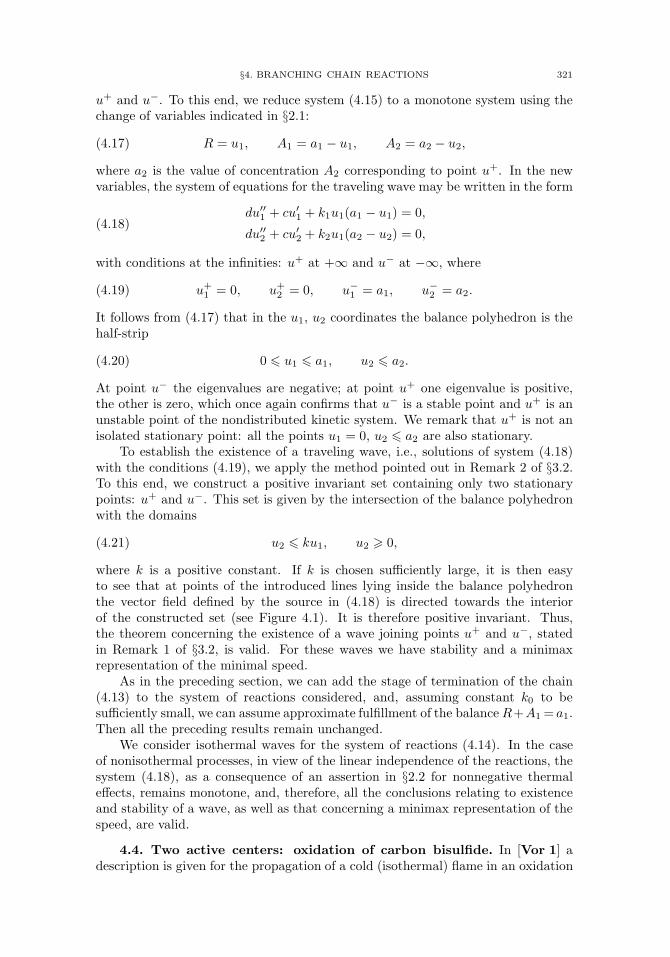
§4. BRANCHING CHAIN REACTIONS 321
u+ and u−. To this end, we reduce system (4.15) to a monotone system using thechange of variables indicated in §2.1:
(4.17) R = u1, A1 = a1 − u1, A2 = a2 − u2,
where a2 is the value of concentration A2 corresponding to point u+. In the newvariables, the system of equations for the traveling wave may be written in the form
(4.18)du′′1 + cu
′1 + k1u1(a1 − u1) = 0,
du′′2 + cu′2 + k2u1(a2 − u2) = 0,
with conditions at the infinities: u+ at +∞ and u− at −∞, where
(4.19) u+1 = 0, u+2 = 0, u−1 = a1, u−2 = a2.
It follows from (4.17) that in the u1, u2 coordinates the balance polyhedron is thehalf-strip
(4.20) 0 u1 a1, u2 a2.
At point u− the eigenvalues are negative; at point u+ one eigenvalue is positive,the other is zero, which once again confirms that u− is a stable point and u+ is anunstable point of the nondistributed kinetic system. We remark that u+ is not anisolated stationary point: all the points u1 = 0, u2 a2 are also stationary.
To establish the existence of a traveling wave, i.e., solutions of system (4.18)with the conditions (4.19), we apply the method pointed out in Remark 2 of §3.2.To this end, we construct a positive invariant set containing only two stationarypoints: u+ and u−. This set is given by the intersection of the balance polyhedronwith the domains
(4.21) u2 ku1, u2 0,
where k is a positive constant. If k is chosen sufficiently large, it is then easyto see that at points of the introduced lines lying inside the balance polyhedronthe vector field defined by the source in (4.18) is directed towards the interiorof the constructed set (see Figure 4.1). It is therefore positive invariant. Thus,the theorem concerning the existence of a wave joining points u+ and u−, statedin Remark 1 of §3.2, is valid. For these waves we have stability and a minimaxrepresentation of the minimal speed.
As in the preceding section, we can add the stage of termination of the chain(4.13) to the system of reactions considered, and, assuming constant k0 to besufficiently small, we can assume approximate fulfillment of the balanceR+A1= a1.Then all the preceding results remain unchanged.
We consider isothermal waves for the system of reactions (4.14). In the caseof nonisothermal processes, in view of the linear independence of the reactions, thesystem (4.18), as a consequence of an assertion in §2.2 for nonnegative thermaleffects, remains monotone, and, therefore, all the conclusions relating to existenceand stability of a wave, as well as that concerning a minimax representation of thespeed, are valid.
4.4. Two active centers: oxidation of carbon bisulfide. In [Vor 1] adescription is given for the propagation of a cold (isothermal) flame in an oxidation
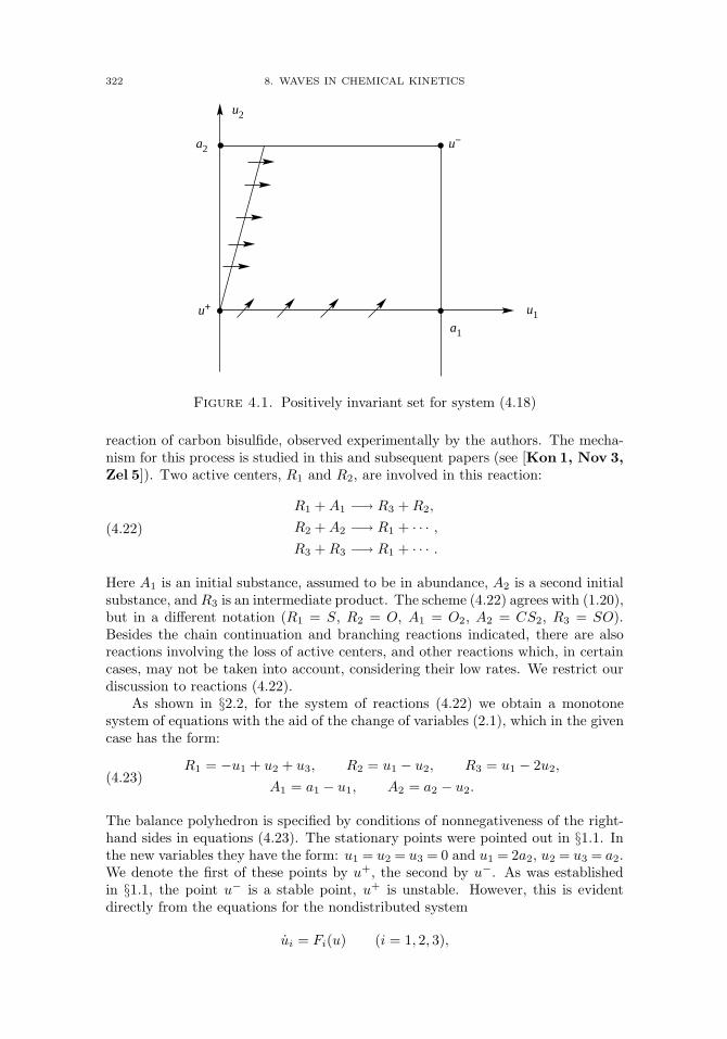
322 8. WAVES IN CHEMICAL KINETICS
a2
u2
a1
u−
u+ u1
Figure 4.1. Positively invariant set for system (4.18)
reaction of carbon bisulfide, observed experimentally by the authors. The mecha-nism for this process is studied in this and subsequent papers (see [Kon 1, Nov 3,Zel 5]). Two active centers, R1 and R2, are involved in this reaction:
(4.22)
R1 +A1 −→ R3 +R2,
R2 +A2 −→ R1 + · · · ,R3 +R3 −→ R1 + · · · .
Here A1 is an initial substance, assumed to be in abundance, A2 is a second initialsubstance, and R3 is an intermediate product. The scheme (4.22) agrees with (1.20),but in a different notation (R1 = S, R2 = O, A1 = O2, A2 = CS2, R3 = SO).Besides the chain continuation and branching reactions indicated, there are alsoreactions involving the loss of active centers, and other reactions which, in certaincases, may not be taken into account, considering their low rates. We restrict ourdiscussion to reactions (4.22).
As shown in §2.2, for the system of reactions (4.22) we obtain a monotonesystem of equations with the aid of the change of variables (2.1), which in the givencase has the form:
(4.23)R1 = −u1 + u2 + u3, R2 = u1 − u2, R3 = u1 − 2u2,
A1 = a1 − u1, A2 = a2 − u2.
The balance polyhedron is specified by conditions of nonnegativeness of the right-hand sides in equations (4.23). The stationary points were pointed out in §1.1. Inthe new variables they have the form: u1 = u2 = u3 = 0 and u1 = 2a2, u2 = u3 = a2.We denote the first of these points by u+, the second by u−. As was establishedin §1.1, the point u− is a stable point, u+ is unstable. However, this is evidentdirectly from the equations for the nondistributed system
ui = Fi(u) (i = 1, 2, 3),
§4. BRANCHING CHAIN REACTIONS 323
where the Fi are reaction rates,
F1 = k1(−u1 + u2 + u3)(a1 − u1),F2 = k2(u1 − u2)(a2 − u2), F3 = k3(u1 − 2u2)2,
Fi are nonnegative functions in the balance polyhedron (cf. (2.12)).Calculation of the eigenvalues at the stationary points leads to the following
result: at the stable point two of the eigenvalues are negative, one is zero; at theunstable point, one eigenvalue is negative, two are zero.
Traveling waves are described by the following system of equations:
du′′i + cu′ + Fi(u) = 0 (i = 1, 2, 3),
with conditions u+ and u− at plus and minus infinity, respectively. This system ismonotone and, therefore, the results obtained above are applicable to it. Namely,for all c ω∗, where ω∗ is obtained with the aid of the minimax representation,there exists a stable traveling wave with speed c. Stability is understood in thesense indicated in §3.2.
As was done above, we can consider nonisothermal processes with nonnegativethermal effects.
4.5. Irreversible reactions. In §§4.2–4.4 we considered models of branchingchain processes in the case of one and two active centers. In this section we considersome examples of branching chain reactions with an arbitrary number n of activecenters in the case of reactions with an open graph.
We begin with the system of reactions
(4.24) Ai + αiRiki−→
n∑j=1
βijRj (i = 1, . . . , n),
where αi > 0. We present conditions under which this system describes a branchingchain process. For this it is sufficient that conditions (4.4) be satisfied; in the givencase, these conditions take the form
(4.25)n∑j=1
βijλj αiλi (i = 1, . . . , n),
where at least one of the inequalities is strict and λj are nonnegative. In matrixform inequalities (4.25) may be written as
(4.26) λγ 0, λγ = 0,
where λ = (λ1, . . . , λn),
(4.27) γ =
β11 − α1 β21 . . . βn1β12 β22 − α2 . . . βn2. . . . . . . . . . . .β1n β2n . . . βnn − αn
.Matrix γ has nonnegative off-diagonal elements. It is necessary that the followingcondition be satisfied:
(4.28) det γ = 0.
Then, for the system of reactions (4.24), Condition 1 of §4.1 is satisfied. Therefore,

324 8. WAVES IN CHEMICAL KINETICS
on the basis of Proposition 4.1, there exists a nondegenerate balance polyhedron Πsuch that the equations
(4.29) R1 = 0, . . . , Rn = 0
specify a stationary point, lying in this polyhedron and being nonattracting. It iseasy to see that polyhedron Π can be specified by the equation
(4.30) R+ γA = µ,
where R = (R1, . . . , Rn), A = (A1, . . . , An), and µ is a vector given by
(4.31) µ = γA0,
where A0 is a given positive vector. It is obvious that A0 is the value of concentra-tion A at the stationary point (4.29).
For the system of reactions (4.24) the monotonicity conditions of §2.2 aresatisfied and the kinetic system may be reduced to a monotone system by thesubstitution (2.1), which in the given case has the form
(4.32) A = A0 − u, R = γu,
where u = (u1, . . . , un).In these variables traveling waves are described by the following system of
equations:
(4.33) du′′ + cu′ + w = 0.
Here w = (w1, . . . , wn) is the vector of the reaction rates:
(4.34) wi = kiAiRαi
i (i = 1, . . . , n).
To the system (4.33) we adjoin the conditions at the infinities:
(4.35) limx→−∞
u(x) = u−, limx→+∞
u(x) = 0.
Thus, at +∞ we have the stationary point (4.29), which is unstable, and at −∞the stationary point u−, which we assume to be stable. A stable stationary pointof a kinetic system exists by virtue of the openness of the graph of the reactions.
We note, as a consequence of (4.33), that all the stationary points of the kineticsystem are determined by the equation
(4.36) w = 0.
By virtue of (4.34), this means that all the stationary points are obtained from theequations
(4.37) AiRi = 0 (i = 1, . . . , n)
and from the condition for these points to belong to the balance polyhedron Π.The property of a point to belong to the balance polyhedron is connected with the
§4. BRANCHING CHAIN REACTIONS 325
choice of vector µ (and, consequently, of A0) appearing in (4.30). For example,consider the stationary point
(4.38) A = 0, R > 0.
It is clear that at this point R = γA0, and, therefore, we obtain a condition on A0
for which the point in question belongs to the balance polyhedron:
(4.39) γA0 > 0.
Similarly, we can also consider other stationary points and determine conditionsunder which they belong to the balance polyhedron Π.
Let conditions (4.39) be satisfied. As u− we select the stationary point (4.38).It follows from (4.32) that u− = A0. It is clear that this point is isolated andasymptotically stable. The latter follows from the fact that for a nondistributedkinetic system we can take, as the Lyapunov function, the function
V = A1 + · · ·+An,
which obviously attains a minimum at the point considered.Thus we can apply to system (4.33) the results of §3 concerning the existence
and stability of waves for monotone systems. Here we need to take into account thepresence of other unstable stationary points. If they are in the balance polyhedron,then when the conditions of Theorem 4.1 of Chapter 3 about the nonexistenceof waves joining unstable stationary points are satisfied, we find that solutions ofproblem (4.33), (4.35) exist. Under certain additional assumptions we can showthat there are no stationary points different from 0 and u− in polyhedron Π.
We pause to consider in more detail the case in which matrix γ is irreducible.In this case, for satisfaction of conditions (4.26), it is necessary and sufficient thatthe eigenvalue of the matrix γ with maximal real part is positive. As λ we can takethe eigenvector corresponding to the eigenvalue with maximal real part. Therefore,for the case in which matrix γ is irreducible, if conditions (4.26) are satisfied wecan take vector λ to be positive and such that inequalities (4.26) are strict.
We can also adduce the following condition.
Proposition 4.2. In order that the system of reactions (4.24) describe abranching process and satisfy Condition 1 of §4.1, it is sufficient that the followinginequality holds :
(4.40) (−1)n−1 det γ > 0.
Proof. It is obvious that the eigenvalue with maximal real part of matrix γ ispositive, since, otherwise, inequality (4.40) would not be satisfied. Satisfaction ofCondition 1 of §4.1 follows form (4.28). This completes the proof of the proposition.
We consider the stationary points of a kinetic system.
Proposition 4.3. If matrix γ is irreducible, then in the intersection G of thebalance polyhedron Π with the interval 0 u u− there are no stationary pointsof the kinetic system different from 0 and u−.
326 8. WAVES IN CHEMICAL KINETICS
Proof. Without loss of generality, we can assume that the reaction rates aregiven by the equations
(4.41) wi = kiAiRi (i = 1, . . . , n),
which follows from (4.37).We assume that in G there is a stationary point u∗, different from 0 and u−.
We show that u∗ > 0. Let us suppose this is not the case and, for definiteness, letu∗i = 0, i = 1, . . . , k < n, and u∗i > 0, i = k + 1, . . . , n. Let us define the functions
ϕi(t) = wi(tu∗) (i = 1, . . . , k).
It is obvious that
(4.42) ϕi(0) = ϕi(1) = 0.
We have
(4.43) ϕ′i(t) =
n∑j=n+1
∂wi(tu∗)∂uj
u∗j .
Since i k < j and the system is monotone, we have ∂wi/∂uj 0, and, consequently,ϕ′i(t) 0 (0 t 1). Together with (4.42), this yields ϕ′
i(t) ≡ 0. Therefore,
(4.44)∂wj(tu∗)∂uj
≡ 0 for 0 t 1, i = 1, . . . , k; j = k + 1, . . . , n.
From (4.41) and (4.42) we obtain
∂wi(tu∗)∂uj
= ki(A0i − tu∗i )γji.
Taking t sufficiently small, from (4.44) we have: γij = 0 (i = 1, . . . , k; j =k + 1, . . . , n). But this contradicts the irreducibility of matrix γ.
We show now that in the polyhedron Π there is an interior point u0 such that
(4.45) u0 u∗, u0i = u∗i for some i.
Indeed, it is obvious that inside Π there exists a point u1 < u∗. We join u1 and u−
by a rectilinear segment. Interior points of this segment lie inside Π. Let u0 be thepoint of intersection of this segment with the boundary of the interval [0, u∗]. Sinceu0 u∗ u− and u∗ = u−, then u0 = u− and is an interior point of Π. By virtueof (4.45), wi(u0) wi(u∗) = 0, since ∂wi/∂uj 0 for i = j. This contradicts thepositiveness of function wi inside Π. The proposition is thereby established.
We proceed now to the problem concerning existence and stability of waves.Based on the proposition just proved and the theorem of §3.2, we can concludethat for all c ω∗, where ω∗ is obtained with the aid of the minimax representa-tion (4.4), (4.5) of Chapter 3, there exist solutions of system (4.33), that are mono-tone with respect to u and satisfy conditions (4.35), for which concentrations A(x)and R(x) are nonnegative. When c < ω∗, such solutions do not exist.
It is easy to see that the matrix ∂wi/∂uj is functionally irreducible and itseigenvalues at point u− are negative. We can therefore apply the results ofChapter 5 concerning the stability of waves in weighted norms. Namely, we denoteby µ+ the eigenvalue with maximal real part of matrix ∂wi/∂uj at zero. Then, asshown in §4 of Chapter 3, we have the inequality ω∗ 2(dµ+)1/2 and the following
§4. BRANCHING CHAIN REACTIONS 327
result concerning stability is valid. If ω∗ > 2(dµ+)1/2, we then have asymptoticstability of waves in weighted norms for all c ω∗. If ω∗ = 2(dµ+)1/2, we thenhave asymptotic stability in weighted norms for c > ω∗. When c = ω∗, the wavesare stable in the sense indicated in §3.2.
A case frequently considered in the study of cold flames is the one in which thereis a deficiency in one of the initial substances and an abundance in the remainingones, and a change in them is neglected in the reaction process. Their concentrationsare then accounted for in the form of rate constant and the reactions scheme (4.24)can be written in the form
(4.46)
A1 + α1R1k1−→
n∑j=1
β1jRj ,
αiRiki−→
n∑j=1
βijRj (i = 2, . . . , n).
We shall assume that inequalities (4.26) and (4.28) remain valid. Then to thesystem of reactions (4.46) there corresponds only the one balance:
(4.47) A1 + (r,R) = A01,
where r = (r1, . . . , rn) is the vector obtained by solving the equation
(4.48) rγ = e1.
Here e1 = (1, 0, . . . , 0), A01 > 0.
Besides the stationary point (4.29):
R = 0, A1 = A01,
which is unstable, there is a second stationary point
(4.49) A1 = 0, r1R1 = A01, Rj = 0 (j = 2, . . . , n),
if r1 > 0.We remark that positiveness of r1 is a necessary condition for boundedness of
the balance polyhedron (4.47), i.e., if r1 0, then it is not bounded. In addition,there is a unique stationary point in the balance polyhedron and it is unstable.It is easy to see that in this case the sum of concentrations of the active centersincreases to infinity in the reaction process. This is a consequence of the fact thatwe have neglected consumption of the initial substances. Thus, for the indicatedchoice of substance which is in short supply, waves do not exist.
Let r1 > 0. Then the stable stationary point is specified by equation (4.49). Itis clear that there are no other stationary points besides the two indicated. Sincethe system may be reduced to a monotone system, conclusions analogous to thepreceding can then be made concerning existence and stability of a wave.
In the system of reactions (4.24) it was assumed that all the substances Ai aredistinct. However, cases are encountered in which the initial substance is consumedin more than one reaction. It can also be the case with the active centers. Herethe condition for reducing a system to a monotone one can be violated, and toprove the existence of a wave, it is necessary to use other methods. It is reasonableto expect that here we can construct a rotation of the vector field and apply theLeray-Schauder method, as was done in Chapters 2, 3, and 9. Instability of a wavein the presence of parallel reactions is possible.
328 8. WAVES IN CHEMICAL KINETICS
4.6. Reversible reactions. The definition of branching chain processes givenin §4.1 also allows the presence of reversible stages.
We consider first the following scheme of reactions:
(4.50)
n∑j=1
αijRj ↔n∑j=1
βijRj ,
A+n∑j=1
αnjRjk−→
n∑j=1
βnjRj ,
i = 1, . . . , n− 1.
For convenience of exposition we begin with the following simple example of sucha scheme:
(4.51) R1k+1←→k−1
R2, R2k+2←→k−2
R3, A+R2k3−→ 2R1.
Here we have only the one balance
A+R1 +R2 +R3 = a (a > 0).
It is easy to find the stationary points
(4.52) R1 = R2 = R3 = 0, A = a
and
(4.53) A = 0, R1 +R2 +R3 = a, k+1 R1 = k−1 R2, k+2 R2 = k−2 R3.
The last equations define a point of detailed equilibrium for the system of reversiblereactions in (4.51). The kinetic system (4.51) has no other stationary points.
The system of reactions considered determines a branching chain process: R1+R2 + R3 increases during the reaction process. Therefore, the point (4.52) isunstable. The stationary point (4.53) is asymptotically stable. This could beverified directly; however, we shall do this in the general case for system (4.50).It follows from what was said in §2 that the system corresponding to (4.51) isreducible to a monotone system. New variables can be introduced with the aid ofequations (2.1):
R1 = −u1 + 2u3, R2 = u1 − u2, R3 = u2 − u3, A = a− u3.
The system of equations for a traveling wave has the form
(4.54) du′′i + cu′i + fi(u) = 0 (i = 1, 2, 3),
where
f1 = k+1 (−u1 + 2u3)− k−1 (u1 − u2),
f2 = k+2 (u1 − u2)− k−2 (u2 − u3),f3 = k3(u2 − u3)(a− u3).
As conditions at the infinities, we specify the stationary points (4.52) and (4.53)in the variables u1, u2, u3. To system (4.54) we can apply the results obtained formonotone systems.
§4. BRANCHING CHAIN REACTIONS 329
We return now to the system of reactions (4.50). We assume that at least onesubstance Rj appears on the left and right sides of the reactions. This means that
n∑j=1
αij > 0,n∑j=1
βij > 0 (i = 1, . . . , n).
We introduce the matrix
γ =
γ11 · · ·γn1. . . . . . . . . .γ1n · · ·γnn
, where γij = βij − αij .
We assume that this matrix is invertible. Condition 1 of §4.1 is then satisfied.Condition (4.4), i.e, a condition sufficient for the system of reactions to describe
a branching chain process, has the form
(4.55)
n∑j=1
λjγij = 0 (i = 1, . . . , n− 1),
n∑j=1
λjγnj > 0, where λj 0 (j = 1, . . . , n).
Without loss of generality, we can assume that λj is a solution of the system ofequations (4.55) and
(4.56)n∑j=1
λjγnj = 1.
This means that the vector λ = (λ1, . . . , λn) is the last row of the matrix γ−1, thematrix inverse to γ. Thus, in order that the system of reactions (4.50) describea branching chain process, it is sufficient that the last row of matrix γ−1 benonnegative.
We construct the balance polyhedron Π. Obviously, it has the form
(4.57) A+n∑j=1
λjRj = A0, A 0, Rj 0,
where λj is a solution of the system (4.55), (4.56), A0 > 0. It is clear that the point
(4.58) R1 = 0, . . . , Rn = 0, A = A0
is a stationary point, and, as follows from Proposition 4.1, it is unstable.We find the other stationary points. To do this, we write down the kinetic
system corresponding to the reactions (4.50):
(4.59)dR
dt= γw,
where w = (w1, . . . , wn), wi = w+i −w−
i , i= 1, . . . , n− 1; w+i , w
−i are the direct and
reverse reaction rates in (4.50), wn is the rate of the last reaction; R= (R1, . . . , Rn).
330 8. WAVES IN CHEMICAL KINETICS
In view of the invertibility of matrix γ, it follows from this that a stationary pointis a solution of the system of equations w = 0, or
(4.60) w+i = w−
i (i = 1, . . . , n− 1), wn = 0.
We consider the stationary point in which A = 0:
(4.61) A = 0,n∑j=1
λjRj = A0, w+i = w−
i (i = 1, . . . , n− 1).
For the existence of such a stationary point it is necessary and sufficient that thissystem have a nonnegative solution Rj (j = 1, . . . , n). On the basis of a well-knownresult (see [Vol 9]) this system has a unique positive solution. This solution is apositive point of detailed equilibrium for the system of reversible reactions in (4.50).
We show that the stationary point (4.61) is asymptotically stable in the balancepolyhedron Π. It follows from known results for reversible reactions (see [Vol 9])that for the system of the first n − 1 reactions in (4.50) the point of detailedequilibrium is asymptotically stable. In addition, the balance plane in which itlies is obviously attracting if the complete system of reactions is considered. Fromthis we can obtain asymptotic stability of point (4.61) for the system of differentialequations corresponding to the reactions (4.50).
Thus we have shown that the nondistributed kinetic system corresponding tothe reactions (4.50) has at least two stationary points: unstable and asymptoticallystable. We can ask the question about the existence of traveling waves joiningthese points. For the case in which the system reduces to a monotone system, themethods presented above can be applied to it. We have illustrated this by thesystem of reactions (4.51). Other examples of this type can also be presented.
In the case considered above the number of intermediate substances Rj is equalto the number of reactions. Using similar methods, we consider the case in whichthe number of intermediate substances is greater than the number of reactions. Welimit the discussion to the following example:
(4.62)R1 +R2
k+1←→k−1
R3,
A+R3k2−→ 2R3.
Here R2 and R3 are active centers; the balance relations are
(4.63)A+R2 +R3 = a2 > 0,
R1 +R2 + 2R3 = a1 > 0.
It is easy to see that Condition 1 of §4.1 is satisfied and that the stationary point
(4.64) A = a2, R1 = a1, R2 = R3 = 0
is unstable. The kinetic system corresponding to the reactions (4.62) is reducible
§4. BRANCHING CHAIN REACTIONS 331
to a monotone system by means of the substitution (2.1), which, in the given case,has the form
R1 = a1 − u1, R2 = 2u2 − u1, R3 = u1 − u2, A = a2 − u2.
Here we obtain the following equations describing traveling waves:
(4.65) du′′i + cu′i + fi(u) = 0 (i = 1, 2),
where
f1(u) = k+1 (a1 − u1)(2u2 − u1)− k−1 (u1 − u2),
f2(u) = k2(a2 − u2)(u1 − u2).
In the variables u1, u2 the polyhedron Π has the form u1 a1, u2 a2, u2 u1 2u2; the unstable point (4.64) is u1 = 0, u2 = 0. There is a second stationary point,which is a point of detailed equilibrium for reversible reactions. It is obtained fromthe equations
u2 = a2, k+1 (a1 − u1)(2u2 − u1) = k−1 (u1 − u2).
We denote it by u−. This point is asymptotically stable. There are no otherstationary points, besides 0 and u−, in polyhedron Π. Thus, traveling waves definedby system (4.65) with the conditions 0 and u− at ±∞ exist and are stable inaccordance with the results for monotone systems presented earlier.
Along with the reactions (4.50), the same methods can be considered forreactions containing more than one irreversible stage.
4.7. Interaction of chains. We have considered branching chain processesfor which there is a single stable stationary point and also unstable stationarypoints. In this section we consider processes for which there exist more than onestable stationary point. This is connected with the presence of more than onebranching chain in the system of reactions and their interaction. The simplestexample exhibiting effects of interest to us is the following:
(4.66)
A1 +R1k1−→ 2R1,
A2 +R2k2−→ 2R2,
R1 +R2k3−→ A1 +A2.
The first and second of these reactions, considered individually, are branching chainreactions, while the third reaction represents an interaction of chains.
For the system of reactions (4.66) we have the balance equations
(4.67) A1 +R1 = a1, A2 +R2 = a2,
where a1 and a2 are positive constants. Taking these balances into account, weobtain the following nondistributed system of equations:
(4.68)R1 = k1R1(a1 −R1)− k3R1R2,
R2 = k2R2(a2 −R2)− k3R1R2 (0 R1 a1, 0 R2 a2).
332 8. WAVES IN CHEMICAL KINETICS
The stationary points are obviously the following:
R1 = 0, R2 = 0,(4.69)
R1 = 0, R2 = a2,(4.70)
R1 = a1, R2 = 0,(4.71)
R1 = r, R2 =k1k3
(a1 − r),(4.72)
wherer =
k1k2a1 − k2k3a2k1k2 − k23
,
assuming that 0 < r < a1.We find conditions for stability of the points (4.70) and (4.71). Direct calcu-
lation of the eigenvalues of the matrix obtained by linearization of the right-handsides of (4.68) at these points leads to the following result: the eigenvalues arenegative if the following inequalities are satisfied:
(4.73)k2k3<a1a2<k3k1.
We note that from these inequalities it also follows that 0 < r < a1. It is also easyto verify that point (4.72) is unstable when conditions (4.73) are satisfied and thatpoint (4.69) is unstable independently of these conditions.
Thus we have shown that when condition (4.73) is satisfied, the kinetic sys-tem (4.68) has four stationary points in the balance polyhedron of which two arestable and two unstable.
It may be verified directly that by means of the substitution R1 = u1, R2 =a2 − u2 the system (4.68) is reduced to a monotone system, which has, as stablestationary points, the points u1 = 0, u2 = 0; u1 = a1, u2 = a2. Thus, a monotonetraveling wave joining these points exists, is unique, and is stable.
We have illustrated the interaction of chains with the simple example (4.66). Asimilar result may also be obtained in a more general case. Let us assume we have asystem of reactions containing two groups of active centers: R(1) = (R(1)
1 , . . . , R(1)k )
and R(2) = (R(2)1 , . . . , R
(2)l ). We assume that there is a subsystem of reactions
with respect to the active centers R(1) and certain intermediate substances A(1),which, for the given subsystem, are initial substances, and that this subsystem,considered independently, describes a branching chain process. In example (4.66)this corresponds to the first reaction. We assume, further, that there is a secondsubsystem of analogous reactions with respect to the active centers R(2) andcertain intermediate substances A(2), which corresponds to the second reactionin example (4.66). We assume, finally, that there is a third subsystem of reactionsin which the active centers from the groups R(1) and R(2) interact, and that, amongthe reaction products, there are the substances A(1) and A(2). This corresponds tothe last reaction in (4.66).
If the first of the indicated subsystems of reactions is considered independently,then, when the conditions indicated in the preceding sections are satisfied, wehave unstable and stable stationary points. Similarly for the second subsystem ofreactions. It proves to be the case that under certain conditions there correspondtwo stable stationary points of the complete system to these two stable stationarypoints for the subsystems.
§5. OTHER MODEL SYSTEMS 333
§5. Other model systems
In addition to the branching chain reactions considered in the preceding section,there are a number of other systems of interest in the applications, which can bestudied with the aid of the methods presented above. We present some of thesehere.
5.1. Belousov-Zhabotinsky reaction. Under certain assumptions travelingwaves in Belousov-Zhabotinsky reactions are described by the following system ofequations (see [Mur 1]):
(5.1)u′′ − cu′ + u(1− u− rv) = 0,
v′′ − cv′ − buv = 0,
where r and b are positive parameters, u 0, v 0.A large number of papers have been devoted to the study of this system of
equations (see [Bel 1, Doc 1, Gib 1, Kan 6, 7, Kla 1, 2, Mur 1, Osc 1, Troy 2,Ye 1], and references therein). We now show how the results of §3 may be appliedto this system of equations.
The system of equations (5.1) is not monotone; however, if we replace u by1− u, we obtain the monotone system of equations
(5.2)u′′ − cu′ + (1− u)(u− rv) = 0,
v′′ − cv′ − b(1− u)v = 0, u 1, v 0.
We find the stationary points of the nondistributed system. We have, obviously,the isolated stationary point
(5.3) u = 0, v = 0
and the half-axis of stationary points
(5.4) u = 1, v 0.
Through linearization of the source it is easy to verify that the stationary point (5.3)is asymptotically stable and that the points (5.4) are unstable for v < 1/r. We limitthe discussion to this case, using the results of §3.
We specify conditions at the infinities for system (5.2) as follows:
(5.5) u(+∞) = 0, v(+∞) = 0, u(−∞) = 1, v(−∞) = v0,
where v0 is an arbitrary number: 0 < v0 < 1/r.As the positively invariant set, such that point (1, v0) is an isolated stationary
point, we can take the set bounded by the lines u=0, v=0, v= v0, v= k(u−1)+v0(see Figure 5.1). Here k is chosen so that bv(u − rv)−1 < k, which can obviouslybe done.
Using the results of §3, we can now state that for each v0, 0 < v0 < 1/r, thereexists a number c∗ > 0, such that for all c c∗ there exists a stable monotonetraveling wave, i.e., a monotone solution of system (5.2) with the conditions (5.5).For c < c∗, no such waves exist. For c∗ we have the minimax representation.
5.2. Heterogeneous-catalytic reactions. In the study of heterogeneous-catalytic reactions we take into account, along with the processes of chemicalkinetics, diffusion, and heat conduction, convective heat and mass transfer. One ofthe models describing these processes leads to the system of equations (1.28), to
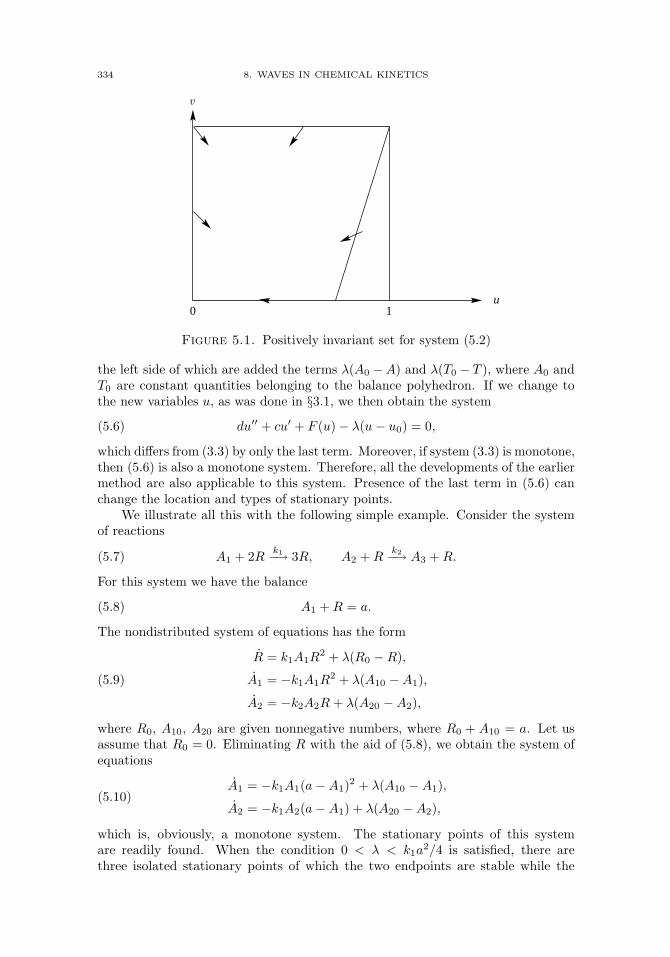
334 8. WAVES IN CHEMICAL KINETICS
1
v
u0
Figure 5.1. Positively invariant set for system (5.2)
the left side of which are added the terms λ(A0 −A) and λ(T0 − T ), where A0 andT0 are constant quantities belonging to the balance polyhedron. If we change tothe new variables u, as was done in §3.1, we then obtain the system
(5.6) du′′ + cu′ + F (u)− λ(u − u0) = 0,
which differs from (3.3) by only the last term. Moreover, if system (3.3) is monotone,then (5.6) is also a monotone system. Therefore, all the developments of the earliermethod are also applicable to this system. Presence of the last term in (5.6) canchange the location and types of stationary points.
We illustrate all this with the following simple example. Consider the systemof reactions
(5.7) A1 + 2R k1−→ 3R, A2 +Rk2−→ A3 +R.
For this system we have the balance
(5.8) A1 +R = a.
The nondistributed system of equations has the form
(5.9)
R = k1A1R2 + λ(R0 −R),
A1 = −k1A1R2 + λ(A10 −A1),
A2 = −k2A2R+ λ(A20 −A2),
where R0, A10, A20 are given nonnegative numbers, where R0 + A10 = a. Let usassume that R0 = 0. Eliminating R with the aid of (5.8), we obtain the system ofequations
(5.10)A1 = −k1A1(a−A1)2 + λ(A10 −A1),
A2 = −k1A2(a−A1) + λ(A20 −A2),
which is, obviously, a monotone system. The stationary points of this systemare readily found. When the condition 0 < λ < k1a
2/4 is satisfied, there arethree isolated stationary points of which the two endpoints are stable while the
BIBLIOGRAPHIC COMMENTARIES 335
intermediate point is unstable. Since the system is monotone, the results obtainedabove can then be applied to it.
5.3. Remarks concerning biological models. Equations of the type con-sidered can describe not only a change of concentration in chemical reactions,but also various biological processes. There is a large literature devoted to theseproblems (see [Bel 1, Mur 1, Rom 1, 2, Svi 2, Volt 1, Zha 1] and referencestherein). We limit the discussion to two examples illustrating the application ofthe methods developed above.
Consider the well-known model for the competition of species
(5.11)u1 = k1u1 − k1u21 − κ1u1u2,
u2 = k2u2 − k2u22 − κ2u1u2.
This system of equations is analogous to the model system (4.68) for the interactionof chains, and its study is entirely similar. Depending on the relationship amongthe parameters, a different number of stationary points is possible here, includingthe presence of two stable stationary points. As was the case in §4.7, replacementof u2 by 1− u2 reduces the system to a monotone system.
As a second example, we consider the biochemical model of Jacob-Monot:
(5.12) u1 = a(1 + u22)−1 − u1, u2 = a(1 + u21)
−1 − u2.
For specified values of parameter a this system has more than one stationary point.Upon replacing u2 by a−u2 (a is a constant), it may also be reduced to a monotonesystem.
For distributed systems corresponding to (5.11) and (5.12) the results concern-ing the existence of waves, their stability, and the representation for the speed arevalid.
Bibliographic commentaries
There is a vast literature devoted to the propagation of chain flames (see [Aza 1,Fran 1, Vor 1, Zel 5], and references therein). However, papers in which mathe-matical modeling of these processes is carried out are few in number. We mentionpapers [Nov 3, 4, Kag 1–4], which are mostly devoted to a numerical analysisof model systems (see also [Cla 2] and references therein). In [Gray 1] numericalstudy of an auto-catalytic system is accompanied by asymptotic analysis. In certaincases, under simplified assumptions, a process permits description by a scalarequation [Vor 1, Nov 3, 4]. A brief description of some of the results presentedin §§4, 5 can be found in [Vol 24, 26].
Literature relating to waves for the Belousov-Zhabotinsky reaction and forbiological models was given previously in §5. There is a number of papers inwhich propagation of waves for heterogeneous-catalytic reactions is discussed (see[Barel 1, Byk 1, Pro 1, Shk 1], and references therein). Traveling waves inchemical kinetics are studied also in [Brow 1, Fei 1, Fife 13, Fre 4, Koro 1,Ter 7, Vol 1, 2].

CHAPTER 9
Combustion Waves with Complex Kinetics
§1. Introduction
In the preceding chapter it was noted that chemical reaction waves, turningone equilibrium state into another, can be divided into two types. The first case,in which both equilibrium states are stationary points of a kinetic system, wasconsidered in Chapter 8. In this chapter we consider combustion waves involving astrong temperature dependence in the reaction rate; this corresponds to the secondcase. As is usual in combustion theory, we assume that the chemical reaction rateis very small at low temperatures in comparison with the maximum temperaturein the combustion wave. In mathematical formulation this means that a “cut-off” is made in the source (see (1.34) in Chapter 8). Thus, in the given case, oneequilibrium state has a kinetic origin while the other is introduced artificially, whichcorresponds to the physical meaning and guarantees that the mathematical modelis well posed.
As we did earlier, let us consider the system of reactions
(1.1)m∑k=1
αikAk →m∑k=1
βikAk, i = 1, . . . , n.
The corresponding system of equations, describing traveling waves, has the form
(1.2)dA′′ + cA′ + ΓΦ(a, T ) = 0,
κT ′′ + cT ′ + (q,Φ(A, T )) = 0.
Here, as usual, A = (A1, . . . , Am) is the vector defining concentrations of thereacting substances, T is the temperature, Φ = (Φ1, . . . ,Φn), Φi is the rate ofthe ith reaction,
(1.3) Φi(A, T ) = ki(T )fi(A), i = 1, . . . , n,
q = (q1, . . . , qn), qi is the adiabatic heating due to the ith reaction, d stands forthe coefficients of diffusion, here assumed all equal, κ is the coefficient of thermaldiffusivity, and c is the wavespeed, which is unknown, as are also the functions A(x)and T (x). Matrix Γ has the form (1.6) of Chapter 8.
At the infinities, the conditions are given by
(1.4)A(+∞) = A+, T (+∞) = T+,
A(−∞) = A−, T (−∞) = T−.
Along with the system of equations (1.2) we shall consider the nondistributed or
337
338 9. COMBUSTION WAVES WITH COMPLEX KINETICS
kinetic system
(1.5)dA
dt= ΓΦ(A, T ),
dT
dt= (q,Φ(A, T ))
and the relations
(sk, A+ −A−) = 0, k = 1, . . . ,m− r,(1.6)
T+ − T− = (p,A+ −A−)(1.7)
(see §1 of Chapter 8), where sk are the vectors forming a complete system of linearlyindependent solutions of the equation
(1.8) skΓ = 0,
and vector p satisfies the equation
(1.9) pΓ = q.
In Chapter 8 we introduced the concept of a reaction with an open graph andwe pointed out the basic properties of such reactions. Recall that in this case weassumed the existence of a vector σ for which the following inequality is valid:
(1.10) σΓ < 0.
(A consequence of (1.9), obviously, is that if all reactions are exothermic, i.e., ifq > 0, then the graph of the reaction is open.) Openness of the graph of a reactionis typical for irreversible reactions, although, of course, not all irreversible reactionshave an open graph.
It is easy to see that the function
(1.11) V (A) = (σ,A)
decreases along trajectories of the kinetic system.We pause briefly to note the contents of this chapter. In §2 the Leray-Schauder
method is used to prove existence of waves for reactions with an open graph. Herewe consider at first the case in which the transport coefficients are equal (κ = d)and thermal effects of the reactions are positive (qi > 0). Next, we waive eitherthe first condition or the second condition. We also consider the problem relatingto the influence of a “cut-off” in the source on the existence of waves. In §3 wepresent a theorem concerning the stability of combustion waves for the case in whichsystem (1.2) is reducible to a monotone system (for κ = d). In the last section wegive examples of reactions that lead to monotone systems.
§2. Existence of waves for kinetic systems with irreversible reactions
In this section we prove the following theorem concerning the existence of wavesfor reaction-diffusion systems.
Theorem 2.1. Suppose the system of reactions (1.1) is given as well as thecorresponding system of equations (1.2), with conditions (1.4) at the infinities,describing a traveling wave. We assume that
1) reaction rates are given by equations (1.3), (2.1);2) A+, T+ is an asymptotically stable stationary point of the kinetic sys-
tem (1.5) in the balance polyhedron Π, A− > 0, and the necessary con-ditions (1.6) and (1.7) for the existence of a wave are satisfied ;

§2. EXISTENCE OF COMBUSTION WAVES 339
3) intermediate stationary points satisfy Condition 1 of §2.1;4) thermal effects of the reactions are positive (qi > 0);5) a cut-off is made in the source, i.e., relations (1.34) of Chapter 8 apply.Then there exists a traveling wave A(x), T (x) joining points A−, T− and A+,
T+, i.e., solutions of system (1.2) with conditions (1.4). Moreover, the concentra-tions A(x) are positive, function V (A(x)), given by equation (1.11), and temperatureT (x) are strictly monotone.
A proof of this theorem is given in §2.4 in the case of equality of transportcoefficients (κ = d); a proof of the general case is given in §2.6. In §2.5 additions tothe theorem are supplied in the case κ = d. A problem considered there concernsthermal effects of different signs (see also the supplement to Part III) and it is alsoshown that if the cut-off is made at different temperatures, we may then have eitherexistence or nonexistence of a wave. In §2.1 we present results that are necessaryfor studying the existence of waves for equations of chemical kinetics; in §§2.2 and2.3 transformations of equations are presented.
2.1. Kinetic system. We consider the system of reactions (1.1). Reactionrates are given in the form (1.3), where
(2.1) fi(A) = Aνi11 × · · · ×Aνim
m gi(A),
νik are arbitrary numbers such that νik 1 if aik = 0, νik = 0 if aik = 0; gi(A) > 0for A 0.
By virtue of condition (1.10), at all stationary points of kinetic system (1.5) wehave the equation
(2.2) Φ(A, T ) = 0.
We consider, in particular, the stationary point A+, T+ at which function V (A)attains a minimum. Suppose that at this point l components of vector A+ vanishand that the remaining components are positive. Since, by assumption, this pointis isolated, we have l r, where r is the rank of matrix Γ. It is easy to see thatwith a small change in the given vector A− > 0 we can arrange to have l becomeequal to r. We shall assume that l = r, and we renumber the substances so thatthe first r substances vanish:
(2.3) A+1 = 0, . . . , A+
r = 0, A+k > 0 (k > r).
Let Γ denote the matrix consisting of the first r rows of matrix Γ, and let Γ be thematrix consisting of its last m− r rows. It follows from the preceding that the rankof matrix Γ is equal to r, and, therefore
(2.4) Γ = RΓ,
where R is a matrix of dimensions (m− r)× r.
Proposition 2.1. Let A, T be an isolated stationary point of system (1.5)and assume that in it exactly r concentrations Ak1 , . . . , Akr equal zero, wherek1, . . . , kr, kr+1, . . . , km is a rearrangement of the numbers 1, . . . ,m. Then for eachsubstance Aki (i = 1, . . . , r), a reaction may be found in which this substance isconsumed and in which the substances Akj (j = i, j = 1, . . . , r) are not consumed.
In view of its simplicity we shall not supply a proof of this proposition.
340 9. COMBUSTION WAVES WITH COMPLEX KINETICS
We apply this proposition to the stationary point A+, T+. Let us renumberthe reactions so that substance Ak is consumed in the kth reaction (k = 1, . . . , r).We denote by Γ0 the matrix consisting of the first r columns and rows of matrix Γ.It then follows from Proposition 2.1 that matrix Γ0 has nonnegative off-diagonalelements.
We assume that the numbers νik appearing in (2.1) satisfy the condition
(2.5) νik 1 (i = 1, . . . , n; k = 1, . . . ,m).
Later on, in proving the existence of waves, we shall get rid of this condition.Let
(2.6) A = (A1, . . . , Ar), A = (Ar+1, . . . , Am).
Then from equation (2.4), for solutions of the kinetic system (1.5) it follows that
(2.7) A = RA+ A+.
From (1.5) it also follows that
(2.8)dA
dt= Ψ(A, T ),
where
(2.9) Ψ(A, T ) = ΓΦ(A, T )
and A is expressed in terms of A from (2.7). It is readily verified directly that
(2.10) Ψ′bA
∣∣∣bA=0
= ΓP,
where matrix P is nonnegative, has nonzero elements in each of its columns, and issuch that matrix ΓP has nonnegative off-diagonal elements.
Proposition 2.2. There exists a vector s > 0 such that
(2.11) sΓ < 0.
All eigenvalues of matrices Γ0 and ΓP lie in the left half-plane.
Proof. From (1.10) and (2.4) we obtain (2.11), where s = σ1 + σ2R, σ =(σ1, σ2). Further, from (2.7) we have (σ,A) = (s, A) + σ2A+. Consequently, (s, A)has a minimum for A = 0 relative to A 0, from which it follows that s > 0.The remaining assertions follow from (2.11) and from the fact that Γ0 and ΓP havenonnegative off-diagonal elements. This completes the proof of the proposition.
It follows from Proposition 2.2 that an arbitrary solution s of inequality (2.11)is positive since matrix Γ0 has an inverse with nonpositive elements. The set ofall solutions s of equation (2.11) forms a cone in r-dimensional space. We considermatrix B, the rows of which are linearly independent vectors of this cone. MatrixB is invertible and positive, and we have the equation
(2.12) BΓ = −K,
where K > 0. Later on, matrix B will be used to reduce system (1.2) to a locallymonotone system.
§2. EXISTENCE OF COMBUSTION WAVES 341
We consider the intermediate stationary points A, T . As already noted, astationary point is characterized by the equations
(2.13) Ak1 = 0, . . . , Aks = 0, Ak > 0 (k = k1, . . . , ks).
We remark that an intermediate point is not asymptotically stable in Π. Indeed,then, it would be an isolated point in Π. Joining A with A+ by a line segment,we find that along this segment, in the direction from A to A+, function V (A)decreases. If we take a point A0 = A lying on this segment, then V (A0) < V (A)and, therefore, the solution of system (1.5) with initial point A0 and correspondingvalue T cannot be attracted to A, T , since V (A) is decreasing along the trajectoriesof system (1.5).
Equations (2.13) define a face of the balance polyhedron Π. The face (2.13) onwhich equation (2.2) is satisfied will be referred to as a stationary face. If it is nota part of another stationary face, we shall call it a maximum stationary face.
Let (2.13) be a maximum stationary face. Let us denote it by Π0. We shallrequire the following condition.
Condition 1. There exists a vector µ such that
(2.14) (µ,A−A) > 0
for all A ∈ Π0, A /∈ Π0, A ∈ Π, and
(2.15) µΓΦ(A, T ) 0
in some neighborhood of face Π0 in Π and corresponding T .
Condition 1 is the condition mentioned in the Introduction. If this conditionis satisfied in the homotopy process, then a wave cannot be “attracted” to anintermediate stationary point. This will be proved in §2.4.
The following condition, more suitable for explicit verification, is sufficient forCondition 1 to be satisfied:
Condition 1′. There exists a vector µ such that µk > 0 for k = kj (j =
1, . . . , s), µk = 0 for k = kj (j = 1, . . . , s), and
(2.16) µΓ 0.
It is not difficult to show that if an intermediate stationary point is isolated inΠ and if inequalities (2.5) are satisfied, then Condition 1 holds for this stationarypoint. If the reactions are independent (r = n), then Condition 1′ holds for theintermediate isolated stationary points, where satisfaction of inequalities (2.5) is nolonger required. We can point out several other examples in which Condition 1 issatisfied. The question as to whether this condition is satisfied for all intermediatepoints in reactions for which (1.10) holds remains open for the present.
In certain cases intermediate stationary points do not exist. Then, naturally,Condition 1 is not needed. This is the case, for example, when r =m, i.e., the rowsof matrix Γ are linearly independent. Then, under the above assumption that thestationary point A+ is isolated, it is a unique stationary point.
2.2. Reduction to a locally monotone system. We show that by a linearchange of the variables A and T system (1.2) can be reduced to a locally monotonesystem (see §2.7 of Chapter 3).
342 9. COMBUSTION WAVES WITH COMPLEX KINETICS
Let us make the change of variables
(2.17) u = BA, θ =T+ − TT+ − T− ,
where A is given by equation (2.6) and matrix B is defined as in (2.12). Theequation for A has, by virtue of (1.2), the form
(2.18) dA′′ + cA′ + ΓΦ(A, T ) = 0,
where Γ is the matrix appearing in (2.4). From this and from (1.2) we obtain, uponusing equations (2.17) and (2.12),
(2.19)du′′ + cu′ −KΦ(u, θ) = 0,
κθ′′ + cθ′ − (q,Φ(u, θ)) = 0.
Here, to avoid introducing new notation, we have denoted function Φ(A, T ) byΦ(u, θ), where A is expressed in terms of u through the relations
(2.20) A = B−1u, A = RB−1u+ A+
(see (2.6) and (2.7)), and T is expressed in terms of θ in accordance with equa-tion (2.17); the quantity q/(T+ − T−) is again denoted by q (in what follows onlythe last value q will be used).
According to (1.4), conditions at the infinities in the new variables have theform
(2.21)u(+∞) = 0, θ(+∞) = 0,
u(−∞) = u−, θ(−∞) = 1,
where
(2.22) u− = BA−.
Denoting by ki(θ) the function ki(T ) in which T is expressed in terms of θ accordingto (2.17), we shall have, in place of (1.34) of Chapter 8,
(2.23)ki(θ) = 0 for θ θ∗,ki(θ) > 0 for θ < θ∗,
i = 1, . . . , n,
where θ∗ is some number:
(2.24) 0 < θ∗ < 1.
Under the assumptions made, function Φ(u, θ) vanishes at the stationary pointsgiven by equation (2.21):
(2.25) Φ(0, 0) = 0, Φ(u−, 1) = 0.
In the new variables equation (1.7) has the form
(2.26) ( p, u−) = 1,
where vector p is defined by the equation
(2.27) pK = q.
Equation (2.26) can also be obtained directly from system (2.19), upon multiplyingthe equation for u by p, subtracting from the equation for θ, and integrating.
§2. EXISTENCE OF COMBUSTION WAVES 343
Matrix B appearing in (2.12) is selected nonuniquely. It is easy to show thatit can be selected so that vector p appearing in (2.27) is a positive vector if q > 0.
Thus, the change of variables (2.17) has led to the system (2.19), which islocally monotone (in the sense of the definition given in §2.7 of Chapter 3) in thedomain where A > 0 provided that thermal effects of the reactions are positive.Indeed, for θ < θ∗ we have Φ(u, θ) > 0 and, therefore, the sources in system (2.19)are negative. When θ θ∗, the sources vanish.
2.3. Change of source. To apply the Leray-Schauder method it is necessaryto change the source in system (2.9) so that at the stationary points u = 0, θ = 0and u = u−, θ = 1 the linearized source will have eigenvalues in the left half-plane.This is done by introducing a small parameter ε > 0 with a subsequent approachto a limit as ε→ 0.
Instead of the function Φi given by equations (1.3), (2.1), we specify thefunctions
Φεi (A, T ) = ki(T )Aµi11 × · · · ×Aµim
m gεi (A)
that are obtained as follows. If νik > 1, then instead of Aνik
k we substitute thefunction Ak(ε + Ak)νik−1. The factor (ε + Ak)νik−1 is included in the functiongεi (A). Thus the functions Φεi (A, T ) have the same form as the functions Φi(A, T ),and the following conditions are satisfied:
µik = 1 for aik > 0, µik = 0 for aik = 0.
Functions Φεi (u, θ) are determined from the functions Φεi (A, T ), as above, with theaid of the substitutions (2.17) and (2.20). Obviously, for ε = 0 we obtain the initialfunctions.
Next, we change the source in a neighborhood of the point u−, 1. To do this,we introduce a smooth function ω(ξ) of the real variable ξ satisfying the conditions:
ω(ξ) =
1 for ξ < δ/2,0 for ξ > δ,
ω′(ξ) < 0 for δ/2 < ξ < δ. Here δ is a sufficiently small number. Instead of (2.19)we consider the system
du′′ + cu′ + f(u, θ) = 0,(2.28)
κθ′′ + cθ′ + g(u, θ) = 0,(2.29)
where
f(u, θ) = −KΦε(u, θ) + εω(|u− − u|)(u− − u),(2.30)
g(u, θ) = ( p, f(u, θ))− εθ + ε( p, u);(2.31)
here vector p is defined by equation (2.27).We also change matrix Γ, replacing βik by βik + ε.Obviously, for ε = 0 system (2.28), (2.29) coincides with the initial sys-
tem (2.19). System (2.28), (2.29) is considered with the conditions (2.21) at theinfinities. It is readily verified that at the points u = 0, θ = 0 and u = u−, θ = 1the linearized source has all eigenvalues in the left half-plane (see Proposition 2.2of §2.1).
344 9. COMBUSTION WAVES WITH COMPLEX KINETICS
2.4. Case of equal transport coefficients (κ = d). In this section we shallprove existence of waves in the case κ = d. Results of this section will be usedlater on. Proof of the existence of waves will be carried out by the Leray-Schaudermethod in a way analogous to that used in Chapter 3. The difference consists inthe fact that the system considered in Chapter 3 was locally monotone over thewhole interval [0, u−], whereas the system considered here is locally monotone onlyin that part of the interval where the concentrations Ak are positive. Therefore weneed to separate solutions monotone with respect to u and positive with respect toA. A priori estimates will be obtained for such solutions.
In the case κ = d the temperature θ can be eliminated from system (2.28). Todo this, we multiply (2.28) by p and subtract from (2.29). Letting
y(x) = θ(x)− ( p, u(x)),
we obtain the equationdy′′ + cy′ − εy = 0.
From (2.21) we obtain, taking into account (2.26),
y(+∞) = 0, y(−∞) = 0.
Consequently, y(x) ≡ 0, i.e.,θ(x) = ( p, u(x))
for all x. We substitute this expression into system (2.28). Setting
(2.32) ϕ(u) = f(u, ( p, u)),
we obtain the system
(2.33) du′′ + cu′ + ϕ(u) = 0
with the following conditions at the infinities:
(2.34) u(+∞) = 0, u(−∞) = 1.
2.4.1. Homotopy. Homotopy is made for an arbitrary sufficiently small fixedε > 0, and, then to prove existence of a wave for ε = 0 we pass to the limit withrespect to ε. It is convenient to describe a homotopy starting from a given system,and moving it to a model system. The existence proof will be carried out in thereverse direction of the homotopy, since here a domain must be constructed alongwhose boundary a rotation is calculated in the application of the Leray-Schaudermethod. The homotopy is carried out in three steps.
First step. We perform a localization of the source in a neighborhood of thestationary points 0 and u−. Homotopy of the source is given by the equation
(2.35)ϕ1τ (u) =− [τ + (1 − τ)ω(|u|)]KΦε(u, θ)
+ εω(|u− − u|)(u− − u) (0 τ 1).
Here, and later in this section, we use the notation
(2.36) θ = ( p, u).
Thus the system considered has the form
(2.37) du′′ + cu′ + ϕ1τ (u) = 0,
§2. EXISTENCE OF COMBUSTION WAVES 345
where, for τ = 0, the source has the form
(2.38) ϕ10(u) = −ω(|u|)KΦε(u, θ) + εω(|u− − u|)(u− − u).
Second step. Before describing the second stage of the homotopy, we note,by virtue of the assumptions, indicated above, connected with isolatedness of thestationary point u = 0, that the source has the form
Φεi (A, T ) = ki(T )Aµir+1r+1 × · · · ×Aµim
m gεi (A)Ai (i = 1, . . . , r).
In accordance with this we make the following homotopy of the source
(2.39)Φεiτ (A, T ) = [(1− τ) + τki(T )Aµir+1
r+1 × · · · ×Aµimm gεi (A)] ×Ai (i = 1, . . . , r),
(2.40) Φεiτ (A, T ) = τΦεi (A, T ) (i = r + 1, . . . ,m).
Thus, for τ = 1 the source Φεiτ coincides with the initial source, and for τ = 0 ithas the form
(2.41) Φεi0(A, T ) = Ai (i = 1, . . . , r), Φεi0(A, T ) = 0 (i > r).
The source ϕ10(u) is homotopied as follows:
(2.42) ϕ2τ (u) = −ω(|u|)KΦετ(u, θ) + εω(|u− − u|)(u− − u) (0 τ 1).
Under such a homotopy the source coincides with (2.38) for τ = 1. For τ = 0 it hasthe form
(2.43) ϕ20(u) = ω(|u|)BΓ0B−1u+ εω(|u− − u|)(u− − u).
The third step consists in effecting a homotopy of matrices B and Γ0 accordingto the formulas
(2.44) Γτ = Γ0τ + (τ − 1)E, Bτ = Bτ + (τ − 1)(Γτ )−1.
Here we obviously have
(2.45) Bτ > 0, BτΓτ < 0.
The source has the form
(2.46) ϕ3τ (u) = ω(|u|)BτΓτ (Bτ )−1 + εω(|uτ− − u|)(uτ− − u),
where
(2.47) uτ− = Bτ A−.
The relationship between variables u and A is given by the equations
(2.48) u = Bτ A, A = RA+A+.
Thus, for τ = 0 we have
(2.49) ϕ30(u) = −ω(|u|)u+ εω(|u0− − u|)(u0− − u).
Thus, in the homotopy process we obtain the system
(2.50) du′′ + cu′ + ϕiτ (u) = 0 (i = 1, 2, 3; 0 τ 1)
346 9. COMBUSTION WAVES WITH COMPLEX KINETICS
with the conditions
(2.51)u(+∞) = 0, u(−∞) = ui,τ− (i = 1, 2, 3),
ui,τ− = u− for i = 1, 2; ui,τ− = uτ− for i = 3.
2.4.2. Separation of solutions monotone with respect to u and positive withrespect to A. We show that there exists a positive number ρ such that
(2.52) ‖uM − uN‖µ ρ.Here uM (x) is an arbitrary solution of system (2.50) for i = 1, 2, 3, 0 τ 1,strictly monotone with respect to x, such that the corresponding concentrationsA(x), given by equations (2.20), are positive; uN(x) is an arbitrary solution ofsystem (2.50) not possessing these properties. We remark that in inequality (2.52)uM and uN can correspond to different τ and i.
We shall use the a priori estimate
(2.53) ‖uM − ψ‖µ Rfor all the indicated solutions uM ; this estimate will be obtained below (§2.4.3). Theconstant R is independent of uM ; ψ is the function introduced in §1 of Chapter 2.
Suppose that the indicated number ρ does not exist. Then we have a sequenceτk → τ0 of values of parameter τ for some i = 1, 2, 3 and sequences ukM and ukN ,such that
(2.54) ‖ukM − ukN‖µ → 0
as k → ∞. Here ukM is the solution of system (2.50) corresponding to τ = τk inwhich c = ck, where ck = c(ukM ) is a value of the functional introduced in §1 ofChapter 2.
It follows from the a priori estimate (2.53) that the sequence ukM is weaklycompact in W 1
2,µ and we can therefore assume it converges weakly to some elementu0 − ψ. By virtue of the fact that ukM is a solution of system (2.50), we find, basedon estimates of operators from below (see §1 of Chapter 2), that ukM − ψ convergesstrongly to u0 − ψ.
Thus
(2.55) ‖ukM − u0‖µ → 0.
Since ukM are solutions of system (2.50) and there are a priori estimates (uniformwith respect to τ) of the first and second derivatives (see §2 of Chapter 3), it followsthat ukM → u0 in C1. It also follows from (2.55) that ck → c0 = c(u0). Thus, u0(x)is a solution of (2.50) for τ = τ0, c = c0.
It follows from (2.54) and (2.55) that
(2.56) ‖ukN − u0‖µ → 0.
As was the case above, it may be proved that ukM → u0 in the C1-norm.To proceed we require a lemma concerning strict positiveness of solutions.
Lemma 2.1. Consider the system
dkA′′k + cA
′k + fk(A)Ak + gk(A) = 0 (k = 1, . . . ,m),
where A = (A1, . . . , Am), dk > 0, fk(A), gk(A) are smooth functions, gk(A) 0 forA 0.
§2. EXISTENCE OF COMBUSTION WAVES 347
Let A(x) be a smooth nonnegative solution of this system on the interval [a, b].Then Ak(x) (k = 1, . . . ,m) are either strictly positive for x ∈ (a, b) or identicallyequal to zero.
Proof. Suppose that Ak(x) 0 and is not identically equal to zero. Considerthe parabolic equation
∂v
∂t= dk
∂2v
∂x2+ ck
∂v
∂x+ fk(A)v + gk(A)
with initial condition
v|t=0 = Ak(x)
and boundary condition
v|x=a = Ak(a), v|x=b = Ak(b).
By the theorem about positiveness of solutions of parabolic equations, v(x, t) > 0.Hence the assertion of the lemma follows since v(x, t) ≡ Ak(x). This completes theproof of the lemma.
Let A0(x) be the function corresponding to the function u0(x) (see (2.20)).Since it is the limit of positive functions, it is nonnegative. Using Lemma 2.1,we show that it is strictly positive. To do this we write equations for A at eachhomotopy step. At the first step it has the form
(2.57) dA′′ + cA′ + [τ + (1− τ)ω(|u|)]ΓΦε(A, T ) + εω(|u− − u|)(A− −A) = 0,
where T is expressed in terms of A in accordance with equations (2.20) and (2.36).At the second homotopy step the equation for A has the form
(2.58) dA′′ + cA′ + ω(|u|)ΓΦετ (A, T ) + εω(|u− − u|)(A− −A) = 0,
where functions Φετ are given by equations (2.39) and (2.40).At the third homotopy step we have
(2.59) dA′′ + cA′ + ω(|u|)Γτ1A+ εω(|uτ− − u|)(A− −A) = 0,
where Γτ1 is a matrix of order m× r, the first r rows of which are formed by rowsof matrix Γτ and the last m− r rows by rows of the matrix RΓτ .
It is easy to see that equations (2.57) satisfy the conditions of Lemma 2.1. Inthe systems (2.58) and (2.59) the first r of the equations, i.e., the equations forA1, . . . , Ar, also satisfy the conditions of Lemma 2.1. Recall that the matrices Γ0and Γτ have non-negative off-diagonal elements. The last m − r equations of sys-tem (2.58) and (2.59) satisfy conditions of Lemma 2.1 outside of a δ-neighborhoodof the point u = 0. Thus we have established positiveness of the function A0(x).
We show that function u0(x) is strictly monotone. It is monotone (possibly,non-strict) as the limit in C1 of monotone functions. Strict monotonicity of thefunction u0(x) follows from the lemma of §2.7 of Chapter 3 since the conditions ofthis lemma are satisfied along solutions u(x) for positive A(x).
348 9. COMBUSTION WAVES WITH COMPLEX KINETICS
Consider now the sequence ukN (x). We show that for sufficiently large k thecorresponding functions Ak(x) are positive. Suppose this not to be the case. Thenthere exists a sequence xk such that
(2.60) Aki (xk) 0
for some i and for some subsequence of values k. Introducing new indexing, we canassume that this holds for all sufficiently large k.
We consider first the case in which xk is a bounded sequence. We can thenassume that xk → x0. Since the sequence Aki (x) converges uniformly to A0
i (x), wethen arrive at a contradiction with the strict positiveness of function A0
i (x).If xk → −∞ along some subsequence, we then arrive at a contradiction since
A−i > 0.
It remains to consider the case in which xk → +∞ along some subsequence.Obviously, the functions Aki (xk) (i = r+1, . . . ,m) are positive for sufficiently largek by virtue of the positiveness of A+
i for i = r + 1, . . . ,m. Consider the functionsAki (x) for i r. To this end, we consider equations (2.57)–(2.59) with respectto A in a sufficiently small neighborhood of point A = 0. From the equationu = Bτ A and the boundedness of matrix Bτ we conclude, for sufficiently small|A|, that ω(|u|) = 1, ω(|uτ− − u|) = 0. Consequently, for sufficiently small |A| theequations (2.57)–(2.59) for A take the form
(2.61) dA′′ + cA′ + ΓΦετ (A, T ) = 0
at the first and second steps of the homotopy and
(2.62) dA′′ + cA′ + Γτ A = 0
at the third step of the homotopy. Let
Mτ = (ΓΦετ (A, T ))′bA
∣∣∣bA=0.
The matricesMτ have nonnegative off-diagonal elements and their eigenvalues withmaximal real parts are negative. Matrix Γτ possesses this very same property;this follows directly from its form (2.44). We can use Lemma 5.3 of Chapter 4,by virtue of which there exists a number x = x, such that if solutions A(x) ofsystem (2.61), (2.62) satisfy conditions A(x) > 0, A(+∞) = 0, we then have theinequality A(x) > 0 for all x > x.
Indeed, consider first the equation (2.61) and let Ψτ (A) = ΓΦετ (A, T ). ThenΨ′τ bA
for A = 0 has positive off-diagonal elements. Let us set
B(x) =∫ 1
0
Ψ′τ bA
(tA) dt,
so that Ψτ (A) =B(x)A. To the system written in this way we now apply Lemma 5.3of Chapter 4. It is easy to see that x can be chosen uniquely for all τ .
For system (2.62) matrix Γτ has positive off-diagonal elements for all τ > 0.When τ = 0 it is equal to −E, but it is easy to see that the assertions of Lemma 5.3of Chapter 4 are valid even in this case.
By virtue of the fact that A 0(x)> 0 and Ak(x) converges to A 0(x), we concludethat for sufficiently large k the inequality A k(x)> 0 holds. Since the function A k(x)
§2. EXISTENCE OF COMBUSTION WAVES 349
satisfies system (2.61) or (2.62) for some τ , it then follows from this that A k(x) > 0for x > x for all sufficiently large k. But this contradicts inequality (2.60) for x > x.
Thus we have shown that functions Ak(x), corresponding to sequence ukN (x),are positive for all sufficiently large k. Hence, according to the definition of thefunctions ukN(x), it follows that they cannot be monotone. This means that thereexists a sequence xk such that
(2.63) (ukNi(x))′ = 0
for some i (here, and in what follows, we have in mind a possible transition tosubsequences).
Sequences xk cannot be bounded since (ukNi(x))′ → u0′(x) uniformly and u0(x)
is a strictly monotone function. Let
(2.64) xk → +∞.
We assume that x0 is so large that u0(x0) lies in a δ-neighborhood of the pointu = 0. This is then the case also for ukN(x) for sufficiently large k. For |u| < δ thefunctions ϕiτ (u) appearing in equation (2.50) are negative for those u to which therecorrespond positive A. Therefore ϕiτ (u
kN (x)) are negative for x > x0 and sufficiently
large k. For xk > x0 it follows from (2.63) that xk is a minimum point of thefunction ukNi(x), more precisely, uk′′Ni(xk) > 0. This follows from equation (2.50) inview of the negativeness of ϕiτ (u). We note that ukNi(x) > 0 since u(x) = BτA(x),A(x)> 0, Bτ > 0. Since ukNi(x)→ 0 as x→∞, for some x > xk the function ukNi(x)attains a maximum, which leads to a contradiction in signs in equation (2.50). Thiscontradiction implies that (2.64) cannot be valid.
It remains only to consider the case
(2.65) xk → −∞.
Let x∗ be such that u0(x) lies in a δ/3-neighborhood of point uτ0− for x < x∗.Recall that τ0 is the value of τ for which u0(x) satisfies system (2.50) (for i = 1, 2,uτ0− = u−). In a δ/2-neighborhood of point uτ− equations (2.50) take the form
(2.66) du′′ + cu′ + ε(uτ− − u) = 0.
For sufficiently large k and x < x∗, function ukN (x) lies in a δ/2-neighborhood ofpoint uτk
− , where τk is that value of τ for which ukN(x) satisfies equation (2.50).This follows from the uniform convergence of ukN (x) to u
0(x) over the whole x-axis.Thus ukN (x) is a solution of equation (2.66) for τ = τk. By virtue of (2.63) ukNi(x)is a constant for all x < x∗. This contradicts the strict monotonicity of functionu0(x).
The contradiction obtained establishes the validity of the statement made atthe beginning of this section concerning the existence of a number ρ such thatinequality (2.52) is valid.
2.4.3. A priori estimates. Here we shall obtain a priori estimates of solutions ofsystem (2.50), monotone with respect to x, and such that the corresponding func-tions A(x) are positive. Monotonicity of the solutions implies boundedness in theC-norm. To obtain estimates in the space W 1
2,µ we need to obtain, as in Chapter 3,a priori estimates of the speed, uniform estimates of solutions in neighborhoods ofpoints 0 and u−, and also to prove that outside of these neighborhoods the solutionis found on a uniformly bounded interval with respect to x. The question concerns
350 9. COMBUSTION WAVES WITH COMPLEX KINETICS
estimates, uniform with respect to τ , in the spaceW 12,µ for fixed (sufficiently small)
ε > 0.Uniform exponential estimates in neighborhoods of points 0 and u− are ob-
tained by the usual methods. They result from the fact that matrices obtained bylinearization of the sources ϕiτ at these points have eigenvalues with negative realparts.
Consider now the question concerning boundedness of the interval with respectto x on which the solution is found outside of these neighborhoods. Violation ofsuch boundedness is only possible in case the solution “is attracted” to interme-diate stationary points u of a kinetic system (see Lemma 2.5 and Lemma 2.8 ofChapter 3). The latter means that corresponding trajectories of the first ordersystem
w′ = p, ap′ = −cp− F (w)
are attracted to the point (u, 0).Stationary points of a kinetic system can be of two types:1. Points at which
(2.67) ki(θ) > 0 (i = 1, . . . , n).
At these points Φi(u, θ) = 0 (i = 1, . . . , n). We note, by virtue of conditions (2.23),that inequality (2.67) is equivalent to the inequality
(2.68) 0 θ < θ∗.
In view of the notation (2.36), this means that we have the inequalities
(2.69) 0 ( p, u) < θ∗.
2. Points at which
(2.70) ki(θ) = 0.
This applies when
(2.71) ( p, u) θ∗.
We consider stationary points of the first kind for which Condition 1 is satisfied(see §2.1). Let this be the point A. We consider only the first homotopy stepsince at the remaining steps there are no intermediate stationary points of the firstkind. We show that in the homotopy process solution A(x) cannot be attracted tostationary point A. Let us assume the contrary. Then there exists a sequence τk,and also a sequence of solutions Ak(x) and a sequence of points xk, such that
(2.72) Ak(xk)→ A.
Here Ak(x) is a solution of system (2.57) for τ = τk. Without loss of generality, wecan assume that τk → τ0.
§2. EXISTENCE OF COMBUSTION WAVES 351
Consider the function
(2.73) yk(x) = (µ,Ak(x)−A),
where µ is a vector appearing in Condition 1. From (2.72) it follows that yk(xk)→ 0.Further, by virtue of Condition 1, we have
(µ,A+ −A) > 0, (µ,A− −A) > 0.
Thus, letting y+ = yk(+∞), y− = yk(−∞), we have
(2.74) y+ > 0, y− > 0.
Consequently, for all sufficiently large k, functions yk(x) reach the smallest valueat some finite point ξk. If this point is not one, we then understand ξk to be thepoint furthest to the left. By virtue of Condition 1, yk(ξk) 0 and therefore
(2.75) yk(ξk)→ 0.
Consider the sequence Ak(ξk). Without loss of generality, we can assume it isconvergent: Ak(ξk) → A∗ as k → ∞. Consequently, by virtue of (2.75) we have(µ,A∗ −A) = 0, and, therefore, on the basis of Condition 1, point A∗ belongs to astationary face Π0. From (2.57) it follows that yk is a solution of the equation
(2.76)dyk
′′+ cyk
′+ [τk + (1− τk)ω(|uk|)]µΓΦε(Ak, T k)
+εω(|u− − uk|)(y− − yk) = 0,
where uk corresponds to Ak. Noting that ξk is the left-most point of the minimumof function yk(x), we obtain a contradiction in signs in equation (2.76) since, byvirtue of Condition 1, for sufficiently large k the source in it is negative. In fact,letting zk(x) = yk(x)−yk(ξk), w(x) = (x−ξ)2, where ξ < ξk and ξk−ξ is sufficientlysmall, we obtain, upon multiplying (2.76) by w and integrating by parts,∫ ξk
ξ
[2d− 2c(x− ξ)]zk(x) dx 0.
This is not possible since zk(x) 0, zk(x) ≡ 0. The contradiction obtained showsthat when Condition 1 is satisfied solution A(x) cannot be attracted to stationarypoint A.
We consider stationary points of the second kind, i.e., points in which equa-tion (2.70) is satisfied. We assume that the thermal effects qi are positive (thermaleffects of different signs will be considered below). Consider first the first homotopystep. If the solution is attracted to an intermediate stationary point, then thereexist two solutions u(1)(x) and u(2)(x) of system (2.50) for i = 1, satisfying thefollowing conditions at the infinities:
limx→∞
u(1)(x) = u(1), limx→−∞
u(1)(x) = u−,
limx→∞
u(2)(x) = 0, limx→−∞
u(2)(x) = u(2) = u−,
where ( p, u(1)) θ∗. In view of the monotonicity of u(1)(x) and the positivenessof vector p, we have the inequality ( p, u(1)(x)) θ∗, from which it follows thatϕ1τ (u
(1)(x)) = 0 for sufficiently large x, and we find, by virtue of Lemma 2.8 ofChapter 3, that c > 0. Similarly, considering solution u(2)(x), we obtain c < 0,
352 9. COMBUSTION WAVES WITH COMPLEX KINETICS
which leads to a contradiction. In the second and third steps of the homotopy wealso arrive at a contradiction in signs of the speed on the basis of Lemma 2.8 ofChapter 3.
Thus, we have shown that when Condition 1 of §2.1 is satisfied, and assumingthermal effects to be positive, the interval with respect to x, outside of neighbor-hoods of points 0 and u−, on which the solution is found is bounded.
A priori estimates of the speed can be obtained in a manner similar to thatused in Chapter 3. But, for the case in question, this can be done more simply ifwe take into account the existence of a domain in the interval [0, u−], separatingthe points 0 and u−, where the source ϕiτ (u) vanishes identically. Indeed, let x1and x2 be such that |u− − u(x1)| = δ, |u− − u(x2)| = δ + ρ, where ρ is chosen sothat ϕiτ (u) = 0 for δ |u− − u| δ + ρ. Then, by virtue of equation (2.50), wehave
d|u′(x2)− u′(x1)| = |c||u(x2)− u(x1)| |c|ρ.
From this and from a priori estimates of derivatives (see Lemma 2.1 of Chapter 3)we obtain an estimate of the speed c.
Thus, under the indicated assumptions, we have obtained an a priori estimateof monotone solutions of system (2.50) to which there correspond positive A.
2.4.4. Existence of waves. To prove existence of a solution of system (2.19) withboundary conditions (2.21), we first carry out such a proof for the system (2.28),(2.29) with the modified source, and we then pass to the limit with ε→ 0.
To prove existence of a solution of system (2.28), (2.29) with conditions (2.21)at the infinities, we apply the Leray-Schauder method, carrying out the previouslydescribed homotopy (§2.4.1).
Consider system (2.50) for τ = 0, i = 3:
(2.77)du′′ + cu′ − ω(|u|)u+ εω(|u0− − u|)(u0− − u) = 0,
u(+∞) = 0, u(−∞) = u0−.
The obtained model system differs from that presented in Chapter 3, and wetherefore treat it independently. A solution of this system has the form
(2.78) u(x) = y(x)u0−,
where y(x) is a scalar function satisfying the equation
(2.79)dy′′ + cy′ − ω(|u0−||y|)y + εω(|u0−||1− y|)(1− y) = 0,
y(+∞) = 0, y(−∞) = 1.
As is well known (see [Kan 3, Fife 7] and Chapter 1), a monotone solution of suchan equation exists and is unique. Thus, a solution of system (2.77) exists. Its mono-tonicity follows from (2.78). We show that a monotone solution of system (2.77)is unique. Indeed, let u(x) be an arbitrary smooth solution of this system. Letvi = ui/u0−i. Then vi satisfies the equation
(2.80)dv′′i + cv
′i − ω(|u(x)|)vi + εω(|u0− − u(x)|)(1 − vi) = 0,
vi(+∞) = 0, vi(−∞) = 1.
In view of the uniqueness of a solution of such a problem, all the vi(x) coincidewith one another, and, therefore, vi(x) = y(x), and u(x) has the form (2.78).
§2. EXISTENCE OF COMBUSTION WAVES 353
System (2.77), linearized on the solution obtained, satisfies the condition forTheorem 5.1 of Chapter 4. From this, as in Chapter 3, we find that a rotation ofthe vector field of the operator corresponding to system (2.77) over a sufficientlysmall ball with center at the stationary point considered is equal to one.
Function A(x) corresponding to the acquired solution u(x) of system (2.77) ispositive. By virtue of equation (2.48), for τ = 0 we have u(x) = A(x). Positivenessof A(x) follows from system (2.59) in view of the fact that A(x) is positive in aδ-neighborhood of points 0 and u0− and outside of these neighborhoods the sourcevanishes and the solution is found explicitly.
Thus we have constructed a domain containing all monotone solutions of system(2.50) (more precisely, stationary points of the corresponding operator) to whichthere correspond positive A(x). This domain contains no solutions not satisfyingthe indicated conditions. A rotation of the vector field over the boundary of thisdomain is equal to unity. Advancing with respect to parameter τ and carrying outconstructions similar to those in Chapter 3, we obtain for the initial system, usinga separation of solutions monotone with respect to u and positive with respect toA, a finite collection of domains containing all solutions of the type indicated aboveand containing no other solutions. A rotation of the vector field over the boundaryof this collection of domains is equal to unity. Existence of solutions of the initialsystem that are monotone with respect to u and positive with respect to A followsfrom this.
We have considered system (2.28), (2.29) for arbitrary sufficiently small ε > 0.It remains now to take the limit as ε → 0. We note that for solutions of thissystem there are a priori estimates in the C-norm, uniform with respect to ε, sinceu(x) is monotone. Uniform estimates in the C1-norm (see §2 of Chapter 3) followfrom this, as well as uniform estimates of the speed (see §2.4.3). As in §2.4.3it may be proved that solutions cannot be attracted to intermediate stationarypoints. Therefore, considering trajectories of the corresponding first order system ofequations, we conclude that there exists a limiting trajectory joining the stationarypoints (0, 0) and (u−, 0). Thus we have proved the existence of monotone solutionsof system (2.19) with conditions (2.21), to which there correspond positive A.
2.5. Additions to the theorem.2.5.1. Thermal effects of different signs. In the theorem we considered the case
in which thermal effects were positive, i.e., q = (q1, . . . , qn)> 0. If these effects wereof different signs, then to obtain a priori estimates and to apply the Leray-Schaudermethod we need to impose an additional condition, which we present below.
If vector q is not positive, then, in general, vector p is also not positive;this vector is a solution of equation (2.27) and specifies a relationship betweentemperature and concentrations in a wave: θ(x) = ( p, u(x)). Therefore, if forpositive thermal effects the temperature in the wave is monotone by virtue ofmonotonicity of u(x), this can then not be the case for thermal effects of differentsigns.
Multiplying equation (2.28) by p, we obtain an equation for θ(x):
dθ′′ + cθ′ − (q,Φ) + εω(|u− − u|)(1− θ) = 0,
θ(−∞) = 1, θ(+∞) = 0,
where (q,Φ) = 0 for θ θ∗ and, by assumption, a δ-neighborhood of point u− lies
354 9. COMBUSTION WAVES WITH COMPLEX KINETICS
in the half-space ( p, u) > θ∗. Therefore, by virtue of the equation, θ(x) 1 for allx.
We require that a positive number ε1 exist such that the following inequalityis satisfied:
(q,Φ(u, θ)) > 0 for θ∗ − ε ( p, u) < θ∗,
where θ = ( p, u). Then, as is readily seen from the equation, function θ(x) ismonotone for θ θ∗ − ε1. Similarly, it may be verified that this function ismonotone in this half-space in the entire homotopy process. Therefore, as was alsothe case for positive thermal effects, the assumption that a solution is attractedto an intermediate stationary point lying in the domain ( p, u) θ∗ leads to acontradiction in signs of the speed. In all other respects, the proof of existence ofsolutions is carried out exactly as before.
2.5.2. Magnitude of cut-off of the source. It is well known that for stage com-bustion processes a wave may not exist; instead, a collection of waves propagatingwith various speeds can appear (see the supplement to Part III). This does notcontradict the theorem for the existence of waves, already proved. This noncorre-spondence is associated with the presence of various time scales in which a processis considered. In a number of cases the time for approach to a wave can be so largethat for a real process one cannot speak about the existence of a wave. Therefore,a more precise description of a process can be obtained by changing somewhat apremise concerning the source.
We consider, as an example, two independent reactions:
A1k1−→ , A2
k2−→ .
We shall assume, in contrast to the case considered in the theorem, that thefunctions ki(θ) vanish, generally speaking, for different temperatures θ = θi. Thesystem of equations for determination of a wave can be written in the form
du′′1 + cu′1 − k1(θ)u1 + εω(|u− − u|)(u−1 − u1) = 0,(2.81)
du′′2 + cu′2 − k2(θ)u2 + εω(|u− − u|)(u−2 − u2) = 0,(2.82)
u(−∞) = u−, u(+∞) = 0,(2.83)
where θ = p1u1 + p2u2, and pi are positive constants. We assume, for simplicity,that u− = (1, 1).
Let us assume, for definiteness, that θ2 θ1 and let us find the stationarypoints of the kinetic system in the half-plane ( p, u) < θ1, different from u = 0 andbelonging to the interval [0, u−]. It is obvious that they must belong to the lineu1 = 0 and lie in the half-plane ( p, u) θ2. Thus, if p2 < θ2, then there are nosuch points. If θ2 p2 < θ1, then these points fill out the interval [θ2/p2, 1] on theaxis of ordinates. If p2 θ1, they then fill out the half-interval [θ2/p2, θ1/p1) onthis same axis.
In case p2 < θ2 or p2 θ1, a solution of system (2.81), (2.82) with the boundaryconditions (2.83) always exists. To prove this, we construct a homotopy of functionkτ1 (θ) in such a way that when τ = 0 it coincides with k1(θ) and vanishes for θ = θτ1 ,where θτ1 = τθ2 + (1 − τ)θ1, 0 τ 1. A priori estimates of monotone solutionscan be obtained here, as was done in the proof of the theorem.
§2. EXISTENCE OF COMBUSTION WAVES 355
Let θ1 > p2 θ2. In this case there exist solutions of system (2.81), (2.82) ofthe form
u1(x) ≡ u1(x), u2(x) ≡ 1, u1(−∞) = 1, u1(+∞) = 0,
u1(x) ≡ 0, u2(x) ≡ u2(x), u2(−∞) = 1, u2(+∞) = 0.
Here ui(x), i = 1, 2, are waves described by the corresponding scalar equation. Wedenote their speeds by c1 and c2, respectively. We note that for p2 = θ2 the solutionu2(x) is not unique: such solutions exist for all c c2, where, in the given case,wavespeed c2 is minimal in absolute value (c2 < 0). For ε = 0, c1 < 0. For smallpositive ε speed c1 changes very little, and, in what follows, the dependence of c1on ε will, for simplicity of exposition, not be taken into account.
We show that for c2 < c1 there exists a wave satisfying conditions (2.83). To dothis, we carry out the homotopy of function kτ1 , described above, with the additionalassumption that kτ1 (θ) k1(θ) for 0 τ 1. It is easy to verify here that if thewave uτ1 exists, then its speed satisfies the inequality cτ1 c1. We need to show thatin the homotopy process the solution cannot be attracted to intermediate pointsfilling out the interval [θ2/p2, 1] of the axis of ordinates. (Otherwise, proof for theexistence of a wave does not change.) If this assertion does not hold, then for someτ and c there exist solutions v(1)(x) and v(2)(x) of system (2.81), (2.82) for whichv(1)(−∞) = u−, v(1)(+∞) = v(1), v(2)(−∞) = v(2), v(2)(+∞) = 0, where pointsv(i), i= 1, 2, belong to the indicated interval. We can show that v(1) = v(2). Indeed,if this is not the case and v(2)2 < v
(1)2 , then for a sequence of prelimiting solutions
u(k)(x) there exist sequences x(1)k and x(2)k , for which
u(k)(x(i)k )→ v(i), u(k)′(x(i)k )→ 0.
(If v(2)2 = θ2/p2, then, instead of the point v(2), it is better to consider thepoint 0.5(v(1) + v(2)) for which such a sequence of values x also exists.) Since( p, u(k)(x(i)k )) > θ2 for large k, it then follows from equation (2.82) that
d[u(k)′
2 (x(2)k )− u(k)′
2 (x(1)k )] + c[u(k)2 (x(2)k )− u(k)2 (x(1)k )] = 0,
which leads to a contradiction as k → ∞ (c = 0). Thus we have shown thatv(1) = v(2).
From the inequality cτ1 > c2 it follows that v(1) cannot coincide with the point(0, 1) (otherwise, cτ1 = c2). If v(1) coincides with some other point of the interval[θ2/p2, 1] of the axis of ordinates, then from equation (2.82) and Lemma 2.6 ofChapter 3, for the solution v(1)(x) we find that c > 0, and for the solution v(2)(x)we find that c < 0. The resulting contradiction shows that the solution cannot beattracted to stationary points on the axis of ordinates. The remaining part of theproof of the existence of waves is the same.
Further, we can show that for c2 c1 no monotone solution of system (2.81),(2.82) with the conditions (2.83) exists. Without going into the details of the proof,we merely indicate its general nature. If the solution indicated above exists, it isthen sufficient to construct a homotopy, in the process of which it cannot disappear
356 9. COMBUSTION WAVES WITH COMPLEX KINETICS
and which converts the initial system into a model system for which such solutionsdo not exist. As such a homotopy, we can take a homotopy kτ2 (θ), for which
k02(θ) ≡ k2(θ), kτ2 (θ) k2(θ)and the value of θτ2 , for which the function kτ2 vanishes, decreases monotonically.Then cτ2 > c2 c1 for τ > 0.
Let F τi denote a nonlinear source in the equation for uτi (x). It is readily verifiedthat for sufficiently small ε we have the estimate∫ 1
0
F τ1 (u1, u2(u1)) du1 < −m1
for an arbitrary monotone function u2(u1) (u2(0) = 0, u2(1) = 1), where m1 is apositive constant (F τ1 ≡ F1). By virtue of the estimate∫ −∞
+∞[uτ
′
1 (x)]2dx m2,
where m2 is a constant which estimates |uτ ′1 (x)| from above (Lemma 2.1 of Chap-ter 3), we obtain an estimate of the speed cτ independent of τ : cτ −m1/m2
(Lemma 2.6 of Chapter 3). On the other hand, for σ > 0 arbitrarily small, forsufficiently small θτ2 , we have∫ 1
0
F τ2 (u1(u2), u2) du2 −σ
for an arbitrary monotone function u1(u2) (u1(0) = 0, u1(1) = 1). In a domainwhere function F τ2 is identically zero, equation (2.82) may be solved explicitly, whichmakes it possible, upon taking into account the acquired estimate from above ofthe speed cτ , to obtain the estimate∫ +∞
−∞[uτ
′
2 (x)]2dx k,
where k is a positive constant independent of τ . By virtue of Lemma 2.6 ofChapter 3 we obtain an estimate of speed cτ −σ/k, which, for small σ, leads toa contradiction with the estimate obtained earlier.
We have thus shown that for c2 c1 a monotone wave cannot exist.Above we have considered the case θ2 θ1. If θ2 > θ1 and θ1 p1 < θ2, then
there exist solutions of system (2.81), (2.82) of the form
u1(x) ≡ 1, u2(x) ≡ u3(x), u2(−∞) = 1, u2(+∞) = 0,
u1(x) ≡ u4(x), u2(x) ≡ 0, u1(−∞) = 1, u1(+∞) = 0.
Here ui(x), i = 3, 4, are waves described by the corresponding scalar equation. Wedenote their speeds by c3 and c4, respectively.
As was done above, it can be proved that for c3 > c4 a monotone solution ofsystem (2.81), (2.82) with conditions (2.83) exists; for c3 c4 such a solution doesnot exist.
We return now to a discussion of various interpretations of the existence ofa wave. We note that Arrhenius temperature dependencies are often taken asthe functions ki(θ). For large activation energies behavior of the process dependsweakly on the size of the cut-off in the source. Therefore, in a mathematical model
§2. EXISTENCE OF COMBUSTION WAVES 357
the size of the cut-off can be specified to a sufficient degree arbitrarily and theresult will depend on this weakly. Thus, if in the example considered above wehave c2 > c1 and θ2 < p2 < θ1, then a wave with the conditions (2.83) does notexist. If θ1 = θ2 > p2 exists, but the corresponding trajectories of the system
w′ = p, ap′ = −cp− F (w)
pass close to the singular point u = (0, 1), p = (0, 0), then the distance betweenlocalized zones of the reaction is so large that in real time it is not the propagationof one wave that is observed, but the propagation of two waves with speeds c1 andc2.
If we consider a wave as an intermediate asymptotics for a source without cut-off [Baren 4], then for the latter the same conclusions remain valid in the exampleconsidered: if c2 c1 or c4 c3, then a wave with the conditions (2.83) does notexist. If c2 < c1 and c4 < c3, then such a wave does exist. These conclusions are inagreement with known results for combustion processes.
2.6. Existence of waves in the absence of equality of transport coef-ficients. Here we establish the existence of waves, i.e., solutions of system (2.19)with boundary conditions (2.21), without assuming that κ = d. In the proof weemploy the Leray-Schauder method, wherein we apply a homotopy to the systemin which κ = d and then make use of the results of the preceding section.
2.6.1. Homotopy. The homotopy will be carried out in three steps. First weconsider ε positive and sufficiently small. This is then followed by a limitingapproach with ε→ 0.
First step. System (2.28), (2.29) is reduced to a system with κ = d. Thehomotopy has the form
du′′ + cu′ + f(u, θ) = 0,(2.84)
κτθ′′ + cθ′ + g(u, θ) = 0,(2.85)
where f and g are given by equations (2.30), (2.31), κτ = (1− τ)d+ τκ, 0 τ 1.Second step. In function f(u, θ) we replace θ by τθ+(1− τ)( p, u). The system
takes the form
du′′ + cu′ + f τ (u, θ) = 0,(2.86)
dθ′′ + cθ′ + gτ (u, θ) = 0,(2.87)
where
f τ (u, θ) = f(u, τθ + (1 − τ)( p, u)),gτ (u, θ) = ( p, f τ(u, θ))− εθ + ε( p, u).
For τ = 0 we have the system (see (2.33)):
du′′ + cu′ + ϕ(u) = 0,(2.88)
dθ′′ + cθ′ + g0(u, θ) = 0,(2.89)
where
(2.90) g0(u, θ) = ( p, ϕ(u))− εθ + ε( p, u),
358 9. COMBUSTION WAVES WITH COMPLEX KINETICS
with the conditions
u(+∞) = 0, u(−∞) = u−,(2.91)
θ(+∞) = 0, θ(−∞) = 1.(2.92)
As a result of the homotopy, we have arrived at system (2.88) considered in §2.4,independent of θ, and at equation (2.89) for θ.
Third step. We carry out a homotopy of system (2.88) in exactly the sameway as was done in §2.4.1. All three steps of the homotopy, described therein, arepresented in the form (2.50), (2.51). In accordance with this, we have the system
du′′ + cu′ + ϕiτ (u) = 0 (i = 1, 2, 3; 0 τ 1),(2.93)
dθ′′ + cθ′ + giτ (u) = 0,(2.94)
where
(2.95) giτ (u) = ( p, ϕiτ (u))− εθ + ε( p, u),
with the conditions
u(+∞) = 0, u(−∞) = ui,τ− ,(2.96)
θ(+∞) = 0, θ(−∞) = ( p, ui,τ− ).(2.97)
We note that equation (2.94) for u, substituted from (2.93), is linear withrespect to θ. At the second and third steps of the homotopy we have
(2.98) θ(x) = ( p, u(x)).
2.6.2. Model system. As a result of the homotopy we have arrived at system(2.93), (2.94) for i = 3, τ = 0. It has the form
du′′ + cu′ + ϕ30(u) = 0,(2.99)
dθ′′ + cθ′ + ( p, ϕ30(u))− εθ + ε( p, u) = 0,(2.100)
where ϕ30(u) is given by equation (2.49) with the conditions
u(+∞) = 0, u(−∞) = u0−,(2.101)
θ(+∞) = 0, θ(−∞) = ( p, u0−).(2.102)
As was shown in §2.4.4, problem (2.99), (2.101) has a unique monotone solutionu(x) to which there corresponds a positive A(x). The solution of problem (2.100),(2.102) is obtained from formula (2.98). Thus, problem (2.99)–(2.102) has a uniquesolution, monotone with respect to x, to which there corresponds a positive A(x).We note, in view of the positiveness of vector p, that function θ(x) given by equation(2.98) is also monotone.
Consider the spectrum of the corresponding linearized problem
du′′ + cu′ +B(x)u = λu, u(±∞) = 0,(2.103)
dθ′′ + cθ′ + ( p,B(x)u)− εθ + ε( p, u) = λθ, θ(±∞) = 0,(2.104)
whereB(x) = [ϕ30(u(x))]
′u.
We note that the matrices, obtained by linearization of the source, have, in the limit
§2. EXISTENCE OF COMBUSTION WAVES 359
as x → ±∞, all eigenvalues with negative real part. Therefore, problem (2.103),(2.104) has, in the half-plane Reλ 0, a discrete spectrum. Further, it followsfrom (2.103), (2.104) that function z = θ − (p, u) satisfies the equation
dz′′ + cz′ − εz = λz, z(±∞) = 0.
For Reλ 0 we obtain z(x) ≡ 0, i.e.,
(2.105) θ(x) = ( p, u(x)).
Since system (2.103) has only the zero solution for λ > 0, and the value λ = 0 is asimple eigenvalue of the system (see Theorem 5.1 of Chapter 4), then, by virtue ofequation (2.105), the same can also be said for the system (2.103), (2.104). (Theabsence of associated vectors in problem (2.103), (2.104) of λ = 0 follows, as canreadily be shown, from the fact of their absence in problem (2.103).)
The indicated properties of the model system will be used in calculating arotation of the vector field at the initial point of the homotopy.
2.6.3. A priori estimates. We now obtain a priori estimates of solutions of thesystem of equations for u and θ, constructed in §2.6.1, at all steps of the homotopy.Here we consider solutions v(x) = (u(x), θ(x)), for which the u(x) are monotonefunctions, the corresponding A(x) are positive, and are such that the temperatureθ(x) at the first homotopy step is a monotone function of x for those values of xfor which |u(x)| δ, |u(x) − u−|2 + |θ(x) − 1|2 δ2. We denote the set of allsuch solutions v(x) by VM . We note that, by virtue of equation (2.98), which holdsat the second and third steps of the homotopy, function θ(x) is monotone on thewhole axis if u(x) is monotone.
We note, further, that the initial equation for θ has the form (2.19) when ε= 0.For positive thermal effects qi and positive A(x) the solution of this equation withcondition (2.21) is monotone in view of the nonnegativeness of function (q,Φ), and,consequently, satisfies the condition
(2.106) 0 θ(x) 1.
Therefore, outside of the interval [0, 1], the values of the functions ki(θ) can bespecified arbitrarily. We shall assume that functions ki(θ) are specified so as tosatisfy the condition
(2.107) ki(θ) = 0 for θ < −1 (i = 1, . . . , n).
Lemma 2.2. At the first homotopy step we have the following estimate for allτ and ε for v ∈ VM :
|θ(x)| 1.
Proof. Let us assume that θ(x) > 1 for some x. Let function θ(x) attain amaximum at point x0. Then at this point θ′′(x0) 0, θ′(x0) = 0; also, by virtue ofequation (2.31),
g(u, θ) εω(|u− − u|)( p, u− − u)− εθ + ε( p, u) ε( p, u−)− εθ = ε(1− θ) < 0.
A contradiction in signs is obtained in equation (2.29).Let us assume that θ(x) < −1, and let x1 be a point at which θ(x) attains its
smallest value. At this point g(u, θ)= εω(|u−−u|)( p, u−−u)−εθ+ε( p, u)−εθ>
360 9. COMBUSTION WAVES WITH COMPLEX KINETICS
ε, θ′′(x1) 0, θ′(x1) = 0, and we have a contradiction in signs in equation (2.29).This completes the proof of the lemma.
Thus we have shown that for all v ∈ VM there is a uniform estimate in theC-norm, independent of ε. As was the case earlier (see §2 of Chapter 3), thisimplies a uniform estimate in the C1-norm, and also a uniform estimate of thespeed (see §2.4.3).
We proceed now to an estimate of solutions v ∈ VM in the norm of W 12,µ for
fixed ε, sufficiently small.Uniform exponential estimates in neighborhoods of the points
u = 0, θ = 0; u = ui,τ− , θ = ( p, ui,τ− )
are obtained by the usual methods. These estimates result from the fact that inlinearizing sources at these points matrices are obtained whose eigenvalues havenegative real parts.
As in §2.4.3, we consider the problem concerning boundedness of the intervalin x on which a solution is obtained outside of these neighborhoods. Violation ofsuch boundedness is only possible in case the solution is attracted to intermediatestationary points of the kinetic system. Here we need to consider only the firsthomotopy step. Indeed, at the third step estimates of u−ψ in the norm ofW 1
2,µ havealready been obtained, while, for θ, an estimate of the difference θ − ( p, ψ) followsfrom equation (2.98). At the second step of the homotopy no further estimates areneeded.
Thus, we consider stationary points of a kinetic system at the first step ofhomotopy, which, obviously, coincide with stationary points of the initial kineticsystem:
(2.108) f(u, θ) = 0, g(u, θ) = 0,
where f and g are given by equations (2.30) and (2.31).It is easy to see that all solutions of equation (2.108), lying in the interval
0 u u−, satisfy the equation θ = ( p, u) and have the form
u = 0, θ = 0,(2.109)
u = u−, θ = 1,(2.110)
|u− − u| δ, θ = ( p, u) for ( p, u) θ∗,(2.111)
Φε(u, θ) = 0, θ = ( p, u) for 0 < ( p, u) < θ∗.(2.112)
Here we assume that δ is chosen so small that the plane ( p, u) = θ∗ in u-space liesoutside of the balls |u− − u| δ, |u| δ.
In a manner similar to what was done in §2.4.3, it may be shown, upon takingmonotonicity of θ(x) into account in the domain indicated above, that the solutioncannot be attracted to the stationary points (2.111) and (2.112). Here, in the courseof the proof, one must consider, instead of the sequenceAk(ξk), the sequenceAk(ξk),θk(ξk), which, as is readily seen, converges to a stationary point.
Thus we have obtained an a priori estimate for v ∈ VM for each fixed, sufficientlysmall ε > 0 and for all 0 τ 1 for all steps of the homotopy:
(2.113) ‖v − ψ‖µ R(ε),
where the constant R is independent of v, and ψ is chosen as in §1 of Chapter 2
§2. EXISTENCE OF COMBUSTION WAVES 361
with the equation θ = ( p, u) taken into account at the second and third steps ofthe homotopy.
2.6.4. Separation of monotone solutions. We show that there exists a constantρ(ε), depending on ε, and such that the following inequality holds:
(2.114) ‖vM − vN‖µ ρ(ε)
for all sufficiently small ε > 0. Here vM ∈ V εM , where V εM is the set of solutionsv(x) = (u(x), θ(x)) for a given ε, indicated in the preceding section (we confineourselves to the first step of the homotopy); vN (x) is an arbitrary solution ofsystem (2.84), (2.85) for a given ε, not belonging to V εM . We denote the set ofall such solutions by V εN . We remark that, as in §2.4.2, vM and vN can be differentsolutions of the indicated equations.
The set V εM is not empty: as we shall show below, for τ = 0 we obtain existenceof solutions of this class as the result of a homotopy in the third and second steps,starting with a model system. The set VN is assumed to be nonempty. Otherwise,the discussion only becomes simpler: there is no need to carry out the indicatedseparation.
Let us assume that the statement formulated above is not true. Then thereexists a sequence εn → 0 and, for arbitrary εn, sequences vnkM ∈ V εn
M and vnkN ∈ V εn
N
and also sequences τnk and τnk (whereby we can assume that τnk→ τn0 as k→∞)such that
(2.115) ‖vnkM − vnkN ‖µ → 0.
Here solutions vnkM correspond to τnk; vnkN correspond to τnk. We can assume, byvirtue of boundedness of speeds, that cnk → cn0, where cnk corresponds to τnk. Itfollows from estimate (2.113) that vnkM −ψ converges weakly to some vn0−ψ ∈W 1
2,µ
(we pass, if necessary, to subsequences). Reasoning as we did in §2.4.2, we find that
(2.116) ‖vnkM − vn0‖µ → 0
as k → ∞. Hence, since vnkM = (unkM , θnkM ) is a solution of system (2.84), (2.85)
and there are a priori estimates (uniform with respect to τ) of the first (see §2.4.3)and, consequently, of the second derivatives, it follows that vnkM → vn0 in C1. Thusvn0 = (un0, θn0) is a solution of system (2.84), (2.85) for τ = τn0, c = cn0.
From (2.115), (2.116) it follows that
(2.117) ‖vnkN − vn0‖µ → 0.
Therefore vnkN → vn0 in the C-norm and therefore in the C1-norm. As in §2.4.2, itmay be shown that function un0(x) is strictly monotone, and the function An0(x),corresponding to it, is strictly positive; also, it may be shown that function unkN ,where vnkN = (unkN , θ
nkN ), is strictly monotone for sufficiently large k, and the function
AnkN (x), corresponding to it, is strictly positive. Hence, it follows from the definitionof set V εN that function θnkN (x) is not monotone for those x for which
|unkN (x)| δ, |unkN (x)− u−|2 + (θnkN (x) − 1)2 δ2.
On the other hand, θn0(x) is monotone in the corresponding domain as the limitof monotone functions θnkM (x). It follows that the function θn0(x) is not strictlymonotone. Letting n tend to infinity, we obtain a contradiction. Indeed, it isnot difficult to show that here vn0 converges along some sequence to the solution
362 9. COMBUSTION WAVES WITH COMPLEX KINETICS
v0 = (u0, θ0) of problem (2.84), (2.85) with boundary conditions (2.21) for someτ = τ0, ε = 0, and c = c0 < 0. Since the source g(u, θ) in equation (2.85) is notpositive for ε= 0, it follows that θ0(x) is a strictly monotone function. On the otherhand, θ0(x) is the limit in the C1-norm of functions θn0(x), not strictly monotoneoutside of the neighborhoods indicated above, and it cannot therefore be strictlymonotone. This contradiction establishes the assertion made at the beginning ofthis section.
2.6.5. Application of the Leray-Schauder method. We assume ε > 0 to be sosmall that inequality (2.114) is valid. Diminishing ρ(ε), if necessary, we can assumethat we do have the separation of monotone solutions obtained in §2.4.2. Thediscussion we follow now parallels that presented in §2.4.4. For a model system(§2.6.2) we construct an operator according to the method indicated in §1 ofChapter 2 and a ball, with center at a stationary point, of sufficiently small radius.A rotation over the boundary of this ball is equal to one. Next, we change τ from0 to 1 in the third step of the homotopy (§2.6.1). We thereby construct domains,similar to those obtained in §2 of Chapter 3, using the separation of solutions,monotone with respect to u and positive with respect to A that was obtainedin §2.4.2. Since equation (2.98) is satisfied here, there correspond monotone θ(x)to monotone u(x). For τ = 1 we arrive at a finite collection of domains D in thespace W 1
2,µ, containing solutions monotone with respect to θ and u and positivewith respect to A, and containing no other solutions. A rotation over the boundaryof these domains is equal to one and, therefore, there exist solutions of the typeindicated.
Next, we go through the second step of the homotopy from τ = 0 to τ = 1,without changing domain D. What we said about this domain above holds byvirtue of equation (2.98). Finally, using separation of monotone solutions obtainedin §2.6.4, we perform the first step of the homotopy from τ =0 to τ =1, constructingdomains separating solutions from VM from other solutions, starting from domainD with τ = 0. For τ = 1 we obtain a domain, a rotation over which is equalto one, implying the existence of solutions from V εM for system (2.28), (2.29) withboundary conditions (2.21).
To complete the proof of the existence of solutions of the initial system (2.19),we take the limit as ε → 0. The arguments are analogous to those presentedin §2.4.4.
§3. Stability of a wave in the case of equality of transport coefficients
In the preceding section we established the existence of a wave for a reaction-diffusion system for a reaction with an open graph, i.e., for the scheme of reac-tions (1.1) for which a solution of inequalities (1.10) exists. In this section weprove the stability of waves in the case of reactions with open graphs under certainassumptions, to be formulated below. We assume the existence of a wave, however,not necessarily under the conditions formulated in §2.
3.1. Reduction to a monotone system. We consider system (1.2) underthe assumption that κ = d and q > 0, with boundary conditions (1.4). In theseconditions A+, T+ is an asymptotically stable stationary point of system (1.5). Aswe did above, we assume that substances are numbered so that A= (A1, . . . , Ar) = 0at this point and that equation (2.7) holds. As in §2.1, we can prove that openness ofthe graph of a reaction implies the existence of a noninvertible nonnegative matrix
§3. STABILITY OF COMBUSTION WAVES 363
B, such that equation (2.12) holds with K 0. Making the substitution (2.17), weobtain system (2.19). Taking into account that κ = d, we can express θ in termsof u (see (2.36)) and reduce system (2.19) to the form
(3.1) du′′ + cu′ −KΦ(A, T ) = 0,
where A, T , and u are connected by the relations (2.17), (2.20), and (2.36). Weshall assume that function Φ has the following form: Φ = (Φ1, . . . ,Φn),
(3.2) Φi(A, T ) = ki(T )Aαi11 · · ·Aαim
m (i = 1, . . . , n),
where k′i(T ) 0, and a cut-off of the form (1.34) of Chapter 8 is made where acut-off at different temperatures is allowed.
Let
(3.3) Ψi(u) = −n∑j=1
KijΦj(A, T ) (i = 1, . . . , r),
where Kij are the elements of matrix K. We have
(3.4)∂Ψi∂uj
= Lij −n∑l=1
Kil∂Φl∂T
∂T
∂uj,
where
(3.5) Lij = −n∑i=1
Kil
m∑l=1
∂Φl∂Ak
∂Ak∂uj
.
It follows from (3.2), the positiveness of vector p and Ak (k = 1, . . . ,m), and thenonnegativeness of Kij that the expression under the summation sign in (3.4) isnonpositive.
Consider (3.5). By virtue of (2.20), we can write
(3.6) A = Su+ (0, A+), S = Γ1Γ−10 B
−1,
where Γ1 is the matrix formed from the first r columns of matrix Γ; Γ0 is thematrix appearing at the intersection of the first r rows and columns of matrix Γ.Invertibility of matrix Γ0 follows from Proposition 2.2. From (3.5) and (3.6) weobtain
(3.7) Lij = −n∑l=1
m∑k=1
KilSkjαlkΦlAk,
where Skj are the elements of matrix S.Thus we have obtained conditions for monotonicity of system (3.1) (cf. §2 of
Chapter 8):If the inequalities
(3.8) KilSkjαlk 0
are satisfied for all i, j = 1, . . . , r, i = j, l = 1, . . . , n, k = 1, . . . ,m, then ∂Φi/∂uj 0 (i = j).
Thus, when conditions (3.8) are satisfied, system (3.1) is monotone.
364 9. COMBUSTION WAVES WITH COMPLEX KINETICS
3.2. Stability. Let us linearize system (3.1) on the traveling wave u(x). Weobtain
(3.9) dv′′ + cv′ + b(x)v = 0, v(±∞) = 0,
where b is a matrix with elements ∂Ψi/∂uj. When conditions (3.8) are satisfied,matrix b(x) has nonnegative off-diagonal elements. By virtue of (3.4), they are notidentically equal to zero since in each row of matrix K there are nonzero elementsand k′i(T ) is not identically zero.
Consider the matrix b+ = lim b(x) as x → ∞. Similarly to what was donein Proposition 2.2, we prove that this matrix has all its eigenvalues in the lefthalf-plane if for each k = 1, . . . , r an i between 1 and n may be found such that∂Φi/∂Ak > 0. This means that for each k = 1, . . . , r a reaction may be found inwhich substance Ak, with stoichiometric coefficient 1, is consumed and the othersubstances Al (l = k, l = 1, . . . , r) are not consumed.
Let L be the operator defined by the left side of equation (3.9). UsingTheorem 5.1 of Chapter 4, we can show that operator L has no eigenvalues inthe half-plane Reλ 0, with the exception of λ = 0, which is a simple eigenvalue.Indeed, let us make the substitution v = exp(µx)y, where µ > 0 is a sufficientlysmall number. We obtain operator L1 = exp(−µx)L exp(µx). Taking into accountthat b(x) ≡ 0 for x < x0, where x0 is some number, and that c < 0, we readilysee that operator L1 satisfies all the conditions of Theorem 5.1 of Chapter 4. Itfollows from this that operator L satisfies items 1) and 2) of the theorem, and, inplace of item 3), we may prove the existence of a bounded positive solution of theadjoint homogeneous equation. From this and from the integrability of a solutionv of equation (3.9) we conclude that 0 is a simple eigenvalue of operator L.
Taking into account the relationship of the stability of a wave to the location ofthe eigenvalues of operator L (see Chapter 5), we arrive at the following theorem.
Theorem 3.1. In system (1.2) let us assume that κ = d, that the thermaleffects qi of the reactions are positive, and that the following conditions are satisfied :
1) inequalities (3.8) are valid ;2) the eigenvalue λ of matrix b+ which has maximal real part is negative;3) a solution A(x), T (x) of system (1.2) with boundary conditions (1.4) exists
such that u(x) = BA(x) is monotone. Here A = (A1, . . . , Ar).Then this solution is stable in the following sense. For an arbitrary solution of
the system of equations
∂T
∂t= κ
∂2T
∂x2+ c∂T
∂x+ (q,Φ),(3.10)
∂A
∂t= d
∂2A
∂x2+ c∂A
∂x+ ΓΦ,(3.11)
with initial conditionsT (x, 0) = T 0(x), A(x, 0) = A0(x),
satisfying the equations
T 0(x) − T+ = ( p,A0(x)−A+),(3.12)
(sk, A0(x) −A+) = 0 (k = 1, . . . ,m− r),(3.13)
§3. STABILITY OF COMBUSTION WAVES 365
where p and sk are given by relations (1.9) and (1.8), the inequality
‖A 0(x) − A(x)‖a εand the condition
(3.14) lim|x|→∞
(A 0(x)− A(x))(1 + e−ax) = 0
imply that
‖T (x, t)− T (x+ h)‖a Me−bt,‖A(x, t)−A(x+ h)‖a Me−bt.
Here ‖ · ‖a is a weighted norm, defined for an arbitrary function g(x) (or vector-valued function) by the equation
‖g‖a = supx|g(x)(1 + e−ax)|,
a is an arbitrary number : 0 < a < |c|/d; ε, M , b are positive numbers independentof the initial condition; h is a constant depending on the initial condition.
Validity of the theorem is a consequence of Theorem 4.1 of Chapter 5.
Remarks. 1) In a condition of the theorem it is assumed that solutions existwith a monotone function u(x). Existence of such solutions was proved in thepreceding section. In the theorem concerning stability it is the fact of the existenceof solutions that is important and not the conditions under which it was obtained.
2) Condition (3.8) is the condition for monotonicity of system (3.1) and is basicto the theorem concerning stability of a wave. It is connected with the choice ofmatrix B, and some arbitrariness in the choice of this matrix makes it possibleto broaden the class of reactions for which stability of traveling waves can beproved. Depending on how matrix B is chosen, satisfaction of inequalities (3.8)can be verified directly. In the following section we show, for linearly independentreactions, how to choose matrix B and we write the conditions (3.8) explicitly interms of stoichiometric coefficients.
3) Matrix b+ has the form BΓPB−1 (see (2.10)). It has nonnegative off-diagonal elements (by virtue of condition (3.8)) and a nonpositive eigenvalue withmaximal real part to which there corresponds a nonnegative eigenvector. In thestatement of the theorem, “something more” is needed. Negativeness of the leadingeigenvalue of matrix b+ is a consequence of Proposition 2.2.
4) In the theorem it is required that an initial perturbation tend towards zeroat the infinities (see (3.14)). For the solution this property is also satisfied for allt > 0.
5) The theorem presented here concerns stability in the space C. Similarly,stability of a wave can be obtained in the spaceW 1
2 (see Theorem 2.2 in Chapter 5).
3.3. Linearly independent reactions. We recall (see §2 of Chapter 8) thatin the case of linearly independent reactions (n= r) the conditions for monotonicitybecome substantially simpler. As matrix B we can take the matrix B = −Γ1
0. Inthis case Γ = Γ0, K =E, the unit matrix, and S =−Γ. Inequality (3.8) assumes theform: γjk 0, if αik > 0 (i = j, i, j = 1, . . . , r; k = 1, . . . ,m). This means that if thekth substance is consumed in the ith reaction, then in any other reaction it mustbe produced with a stoichiometric coefficient at least equal to its stoichiometric
366 9. COMBUSTION WAVES WITH COMPLEX KINETICS
coefficient in the ith reaction. For example, if the kth substance is consumed intwo reactions, the ith and the jth, the inequalities γik 0 and γjk 0 must thenbe satisfied.
It is obvious that the conditions mentioned will be satisfied, in particular, ifeach substance is consumed in no more than one reaction.
§4. Examples
In this section the results presented above on the existence and stability ofwaves are illustrated through typical examples. We note that the monotonicityconditions discussed in Chapter 8 and in the preceding sections of this chapterexhibit an unconditional character. For example, for linearly independent reactionsin which each substance is consumed in at most one reaction, the system may bereduced to a monotone system independently of the values of the parameters. Butif there are competing stages in the reaction scheme, the system can also be reducedto a monotone system, but upon satisfaction of certain conditions. This questionhas not been discussed for a reaction scheme of a general type; it will be consideredin the examples to be presented.
4.1. Single-stage reactions. This case has been studied in the literature indetail (see, for example, [Zel 5]); it is presented here for completeness.
A solution of traveling-wave type for the single-stage chemical reaction
α1A1 + · · ·+ αmAm → β1A1 + · · ·+ βmAm,
accompanied by the liberation of heat, satisfies the system of equations
κT ′′ + cT ′ + qF (A1, . . . , Am, T ) = 0,(4.1)
djA′′j + cA
′j + γjF (A1, . . . , Am, T ) = 0, j = 1, . . . ,m,(4.2)
where F is the reaction rate, usually considered in the form
F (A1, . . . , Am, T ) = k(T )Aα11 × · · · ×Aαm
m
(law of mass action), γj = βj − αj . If the coefficients of diffusion are all equal(dj = d, j = 1, . . . ,m), then, as is readily seen,
Aj =γjγ1A1 + αj , j = 1, . . . ,m,
where the aj are constants (it is assumed that γ1 = 0). If, in addition, the coefficientof thermal conductivity κ is equal to the coefficient of diffusion d (similarity ofconcentration and temperature fields), then
T =q
γ1A1 + T+,
where T+ is a constant. In this case the system of equations (4.1), (4.2) may bereduced to a scalar equation for which questions of existence and stability of wavesare answered fairly easily (see Chapter 1). The type of source, characteristic incombustion, is shown in Figure 1.3 of the Introduction. For this source a waveexists, is unique, and is stable.
The situation is substantially more involved if κ = d. Existence of waves andtheir uniqueness was established in [Kan 4] for d < κ. It was shown in [Bac 1]that for d > κ, and for specially selected conditions, a wave can be nonunique (see
§4. EXAMPLES 367
also [Bon 2]). From the general theorem presented in §2 the existence of wavesfollows directly; however, the theorem does not permit any judgement concerningthe number of such waves. We note also that the Leray-Schauder method can beused to establish the existence of waves even when the coefficients of diffusion arenot all equal to one another.
A large number of papers (see the supplement to this Part) has been devotedto the stability of waves of combustion in the case of a single-stage reaction withκ = d. This problem will not be considered here.
As a rule, chemical reactions are many-stage reactions, i.e., they consist not ofa single reaction, as in the preceding example, but of a large number of reactions.We consider such reactions in the following examples.
4.2. Independent reactions. By independent reactions we mean reactionsin which the substances being consumed are used up in only one reaction and arenot produced in any reaction. For the general reaction scheme (1.1) this meansthat if αi0j0 = 0, then
αij0 = 0, i = i0, βij0 = 0, i = 1, . . . , n.
For simplicity, we limit the discussion here to an example of three bimolecularreactions:
A1 +A2k1−→ · · · , A3 +A4
k2−→ · · · , A5 +A6k3−→ · · · ,
since all that follows carries over, in an obvious way, to an arbitrary numberof independent reactions, an arbitrary number of substances taking part in eachreaction, and to arbitrary stoichiometric coefficients.
We note that the reaction rate does not depend on the substances being formed(since these substances do not include A1, . . . , A6). Therefore, it is not necessaryto consider the right sides of the reactions.
The complete system of equations of heat conduction and diffusion has, on theassumption of equality of the diffusion coefficients, the form
κT ′′ + cT ′ + q1k1(T )A1A2 + q2k2(T )A3A4 + q3k3(T )A5A6 = 0,
dA′′1 + cA′
1 − k1(T )A1A2 = 0,
dA′′2 + cA′
2 − k1(T )A1A2 = 0,...........................
dA′′6 + cA′
6 − k1(T )A5A6 = 0.
Going over to the vector matrix form of notation (see (1.2)), we can write theequation for the concentrations in the form
dA′′ + cA′ + ΓF = 0,
where F = (F1, F2, F3), A = (A1, . . . , A6),
F1 = k1(T )A1A2, F2 = k2(T )A3A4, F3 = k3(T )A5A6,
Γ =
−1 0 0−1 0 00 −1 00 −1 00 0 −10 0 −1
.
368 9. COMBUSTION WAVES WITH COMPLEX KINETICS
It is easy to see that the graph of the reaction is open since λΓ < 0 for vectorλ, made up, for example, of ones (which corresponds to the sum of the rows of thematrix). The reactions are linearly independent, i.e., the columns of matrix Γ arelinearly independent, and there are balances, i.e., the rows of matrix Γ are linearlydependent. The balances have the form
A2 = A1 + a1, A4 = A3 + a2, A6 = A5 + a3,
where a1, a2, a3 are constants, which, without loss of generality, we can assume tobe positive. In this case the balance polyhedron Π is specified by the inequalitiesA1 0, A3 0, A5 0. It contains the asymptotically stable stationary pointA1 = A3 = A5 = 0 and no other stationary points of the kinetic system.
Thus, if the thermal effects qi, i = 1, 2, 3, of the reactions are positive, all theconditions of the theorem for the existence of waves are satisfied (for an appropriatespecification of the conditions at the infinities and a “cut-off” of the source).
For independent reactions the conditions for reduction of the system to amonotone system in the case κ = d are also satisfied (each substance is consumedin at most one reaction; see §3.3). Using the change of variables described in §3.3,which in the given case has the form
A1 = u1, A3 = u2, A5 = u3,
we obtain the system of equations
du′′i + cu′i − ki(T )ui(ui + ai) = 0,
where T =T+−q1u1−q2u2−q3u3. This system is, obviously, monotone if k′i(T ) 0(≡ 0) and the wave in this case is stable, both with respect to small perturbationsand globally (in the case of monotone initial conditions), is unique, and the minimaxrepresentation of the speed applies.
4.3. Sequential reactions. We consider examples of reactions in which eachsubstance is consumed in at most one reaction, and in each reaction, except for thefirst, the substance consumed is that formed in the preceding reaction.
As we did before, we limit the discussion to simple examples, which can beeasily generalized.
We consider sequential reactions of the form
(4.3) A1k1−→ A2, A2
k2−→ A3, A3k3−→ A4.
Reactions (4.3) are linearly independent and, consequently, the graph of reactionis open. The corresponding system of equations has the form
κT ′′ + cT ′ +3∑i=1
qiFi = 0,
dA′′ + cA′ + ΓF = 0,
where
A = (A1, A2, A3), F = (F1, F2, F3), Fi = ki(T )Ai,
Γ =
−1 0 01 −1 00 1 −1
.
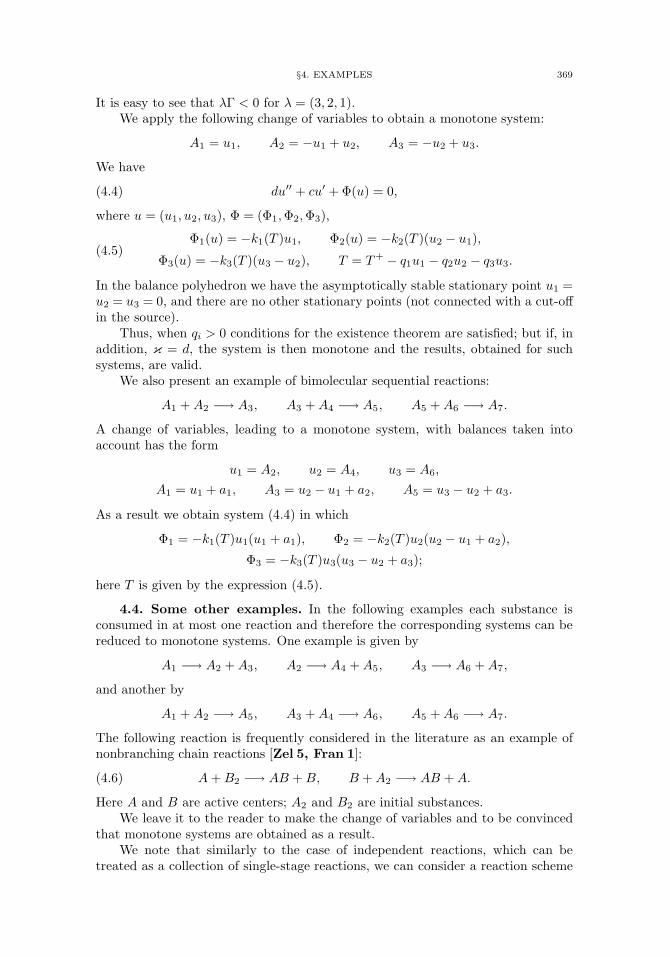
§4. EXAMPLES 369
It is easy to see that λΓ < 0 for λ = (3, 2, 1).We apply the following change of variables to obtain a monotone system:
A1 = u1, A2 = −u1 + u2, A3 = −u2 + u3.
We have
(4.4) du′′ + cu′ +Φ(u) = 0,
where u = (u1, u2, u3), Φ = (Φ1,Φ2,Φ3),
(4.5)Φ1(u) = −k1(T )u1, Φ2(u) = −k2(T )(u2 − u1),
Φ3(u) = −k3(T )(u3 − u2), T = T+ − q1u1 − q2u2 − q3u3.
In the balance polyhedron we have the asymptotically stable stationary point u1 =u2 = u3 = 0, and there are no other stationary points (not connected with a cut-offin the source).
Thus, when qi > 0 conditions for the existence theorem are satisfied; but if, inaddition, κ = d, the system is then monotone and the results, obtained for suchsystems, are valid.
We also present an example of bimolecular sequential reactions:
A1 +A2 −→ A3, A3 +A4 −→ A5, A5 +A6 −→ A7.
A change of variables, leading to a monotone system, with balances taken intoaccount has the form
u1 = A2, u2 = A4, u3 = A6,
A1 = u1 + a1, A3 = u2 − u1 + a2, A5 = u3 − u2 + a3.
As a result we obtain system (4.4) in which
Φ1 = −k1(T )u1(u1 + a1), Φ2 = −k2(T )u2(u2 − u1 + a2),Φ3 = −k3(T )u3(u3 − u2 + a3);
here T is given by the expression (4.5).
4.4. Some other examples. In the following examples each substance isconsumed in at most one reaction and therefore the corresponding systems can bereduced to monotone systems. One example is given by
A1 −→ A2 +A3, A2 −→ A4 +A5, A3 −→ A6 +A7,
and another by
A1 +A2 −→ A5, A3 +A4 −→ A6, A5 +A6 −→ A7.
The following reaction is frequently considered in the literature as an example ofnonbranching chain reactions [Zel 5, Fran 1]:
(4.6) A+B2 −→ AB +B, B +A2 −→ AB +A.
Here A and B are active centers; A2 and B2 are initial substances.We leave it to the reader to make the change of variables and to be convinced
that monotone systems are obtained as a result.We note that similarly to the case of independent reactions, which can be
treated as a collection of single-stage reactions, we can consider a reaction scheme
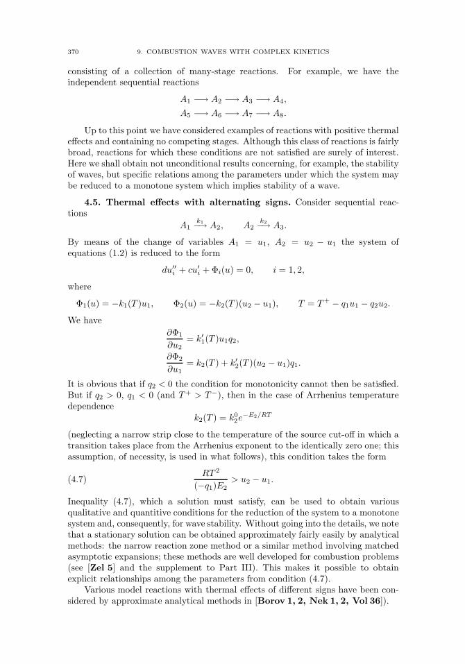
370 9. COMBUSTION WAVES WITH COMPLEX KINETICS
consisting of a collection of many-stage reactions. For example, we have theindependent sequential reactions
A1 −→ A2 −→ A3 −→ A4,
A5 −→ A6 −→ A7 −→ A8.
Up to this point we have considered examples of reactions with positive thermaleffects and containing no competing stages. Although this class of reactions is fairlybroad, reactions for which these conditions are not satisfied are surely of interest.Here we shall obtain not unconditional results concerning, for example, the stabilityof waves, but specific relations among the parameters under which the system maybe reduced to a monotone system which implies stability of a wave.
4.5. Thermal effects with alternating signs. Consider sequential reac-tions
A1k1−→ A2, A2
k2−→ A3.
By means of the change of variables A1 = u1, A2 = u2 − u1 the system ofequations (1.2) is reduced to the form
du′′i + cu′i +Φi(u) = 0, i = 1, 2,
where
Φ1(u) = −k1(T )u1, Φ2(u) = −k2(T )(u2 − u1), T = T+ − q1u1 − q2u2.
We have∂Φ1
∂u2= k′1(T )u1q2,
∂Φ2
∂u1= k2(T ) + k′2(T )(u2 − u1)q1.
It is obvious that if q2 < 0 the condition for monotonicity cannot then be satisfied.But if q2 > 0, q1 < 0 (and T+ > T−), then in the case of Arrhenius temperaturedependence
k2(T ) = k02e−E2/RT
(neglecting a narrow strip close to the temperature of the source cut-off in which atransition takes place from the Arrhenius exponent to the identically zero one; thisassumption, of necessity, is used in what follows), this condition takes the form
(4.7)RT 2
(−q1)E2> u2 − u1.
Inequality (4.7), which a solution must satisfy, can be used to obtain variousqualitative and quantitive conditions for the reduction of the system to a monotonesystem and, consequently, for wave stability. Without going into the details, we notethat a stationary solution can be obtained approximately fairly easily by analyticalmethods: the narrow reaction zone method or a similar method involving matchedasymptotic expansions; these methods are well developed for combustion problems(see [Zel 5] and the supplement to Part III). This makes it possible to obtainexplicit relationships among the parameters from condition (4.7).
Various model reactions with thermal effects of different signs have been con-sidered by approximate analytical methods in [Borov 1, 2, Nek 1, 2, Vol 36]).
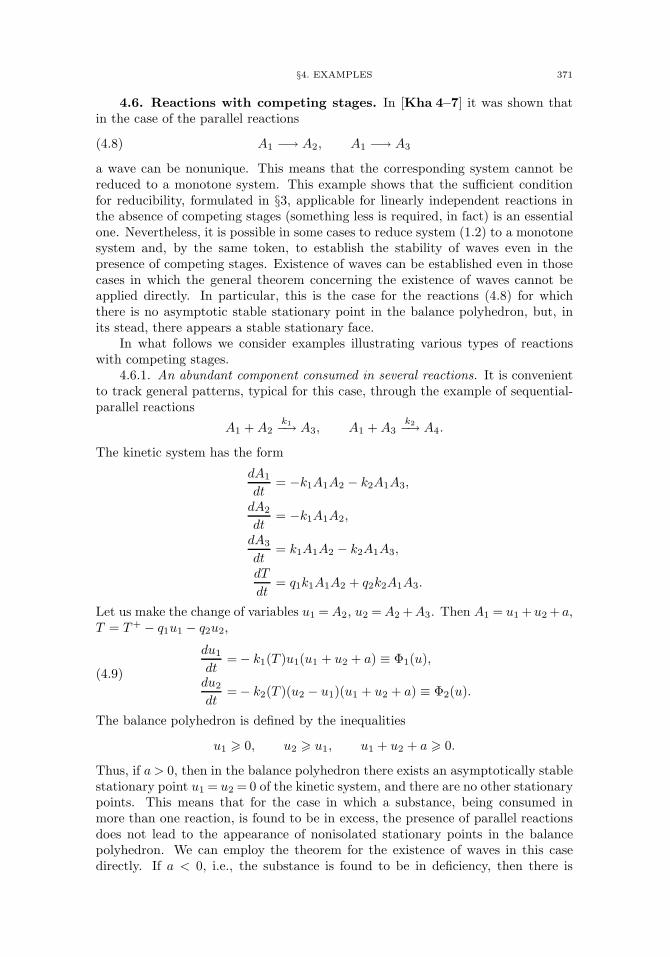
§4. EXAMPLES 371
4.6. Reactions with competing stages. In [Kha 4–7] it was shown thatin the case of the parallel reactions
(4.8) A1 −→ A2, A1 −→ A3
a wave can be nonunique. This means that the corresponding system cannot bereduced to a monotone system. This example shows that the sufficient conditionfor reducibility, formulated in §3, applicable for linearly independent reactions inthe absence of competing stages (something less is required, in fact) is an essentialone. Nevertheless, it is possible in some cases to reduce system (1.2) to a monotonesystem and, by the same token, to establish the stability of waves even in thepresence of competing stages. Existence of waves can be established even in thosecases in which the general theorem concerning the existence of waves cannot beapplied directly. In particular, this is the case for the reactions (4.8) for whichthere is no asymptotic stable stationary point in the balance polyhedron, but, inits stead, there appears a stable stationary face.
In what follows we consider examples illustrating various types of reactionswith competing stages.
4.6.1. An abundant component consumed in several reactions. It is convenientto track general patterns, typical for this case, through the example of sequential-parallel reactions
A1 +A2k1−→ A3, A1 +A3
k2−→ A4.
The kinetic system has the form
dA1
dt= −k1A1A2 − k2A1A3,
dA2
dt= −k1A1A2,
dA3
dt= k1A1A2 − k2A1A3,
dT
dt= q1k1A1A2 + q2k2A1A3.
Let us make the change of variables u1 =A2, u2 =A2+A3. Then A1 = u1+u2+ a,T = T+ − q1u1 − q2u2,
(4.9)
du1dt
=− k1(T )u1(u1 + u2 + a) ≡ Φ1(u),
du2dt
=− k2(T )(u2 − u1)(u1 + u2 + a) ≡ Φ2(u).
The balance polyhedron is defined by the inequalities
u1 0, u2 u1, u1 + u2 + a 0.
Thus, if a > 0, then in the balance polyhedron there exists an asymptotically stablestationary point u1 = u2 = 0 of the kinetic system, and there are no other stationarypoints. This means that for the case in which a substance, being consumed inmore than one reaction, is found to be in excess, the presence of parallel reactionsdoes not lead to the appearance of nonisolated stationary points in the balancepolyhedron. We can employ the theorem for the existence of waves in this casedirectly. If a < 0, i.e., the substance is found to be in deficiency, then there is
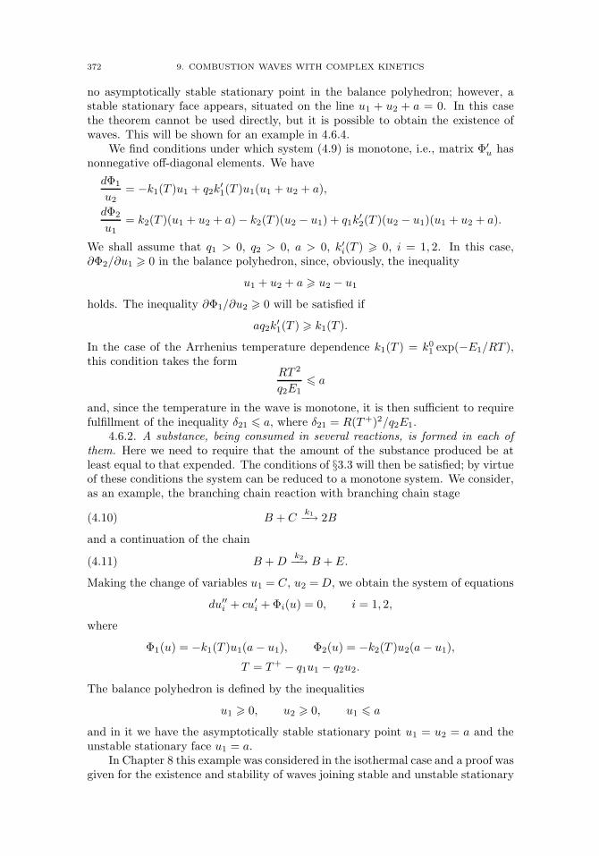
372 9. COMBUSTION WAVES WITH COMPLEX KINETICS
no asymptotically stable stationary point in the balance polyhedron; however, astable stationary face appears, situated on the line u1 + u2 + a = 0. In this casethe theorem cannot be used directly, but it is possible to obtain the existence ofwaves. This will be shown for an example in 4.6.4.
We find conditions under which system (4.9) is monotone, i.e., matrix Φ′u has
nonnegative off-diagonal elements. We havedΦ1
u2= −k1(T )u1 + q2k′1(T )u1(u1 + u2 + a),
dΦ2
u1= k2(T )(u1 + u2 + a)− k2(T )(u2 − u1) + q1k′2(T )(u2 − u1)(u1 + u2 + a).
We shall assume that q1 > 0, q2 > 0, a > 0, k′i(T ) 0, i = 1, 2. In this case,∂Φ2/∂u1 0 in the balance polyhedron, since, obviously, the inequality
u1 + u2 + a u2 − u1holds. The inequality ∂Φ1/∂u2 0 will be satisfied if
aq2k′1(T ) k1(T ).
In the case of the Arrhenius temperature dependence k1(T ) = k01 exp(−E1/RT ),this condition takes the form
RT 2
q2E1 a
and, since the temperature in the wave is monotone, it is then sufficient to requirefulfillment of the inequality δ21 a, where δ21 = R(T+)2/q2E1.
4.6.2. A substance, being consumed in several reactions, is formed in each ofthem. Here we need to require that the amount of the substance produced be atleast equal to that expended. The conditions of §3.3 will then be satisfied; by virtueof these conditions the system can be reduced to a monotone system. We consider,as an example, the branching chain reaction with branching chain stage
(4.10) B + C k1−→ 2B
and a continuation of the chain
(4.11) B +D k2−→ B + E.
Making the change of variables u1 = C, u2 =D, we obtain the system of equations
du′′i + cu′i +Φi(u) = 0, i = 1, 2,
where
Φ1(u) = −k1(T )u1(a− u1), Φ2(u) = −k2(T )u2(a− u1),T = T+ − q1u1 − q2u2.
The balance polyhedron is defined by the inequalities
u1 0, u2 0, u1 aand in it we have the asymptotically stable stationary point u1 = u2 = a and theunstable stationary face u1 = a.
In Chapter 8 this example was considered in the isothermal case and a proof wasgiven for the existence and stability of waves joining stable and unstable stationary
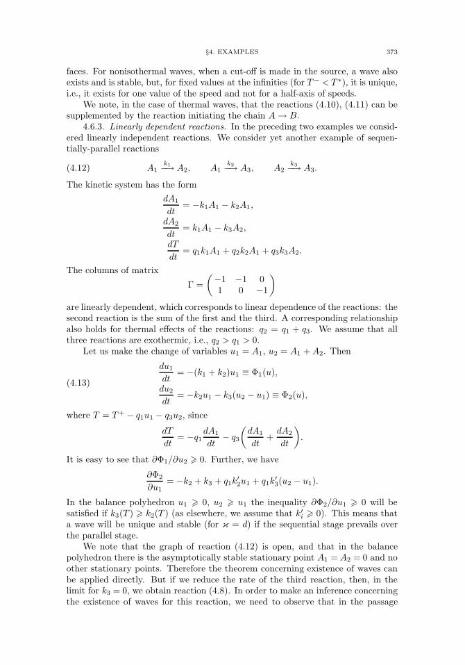
§4. EXAMPLES 373
faces. For nonisothermal waves, when a cut-off is made in the source, a wave alsoexists and is stable, but, for fixed values at the infinities (for T− < T ∗), it is unique,i.e., it exists for one value of the speed and not for a half-axis of speeds.
We note, in the case of thermal waves, that the reactions (4.10), (4.11) can besupplemented by the reaction initiating the chain A→ B.
4.6.3. Linearly dependent reactions. In the preceding two examples we consid-ered linearly independent reactions. We consider yet another example of sequen-tially-parallel reactions
(4.12) A1k1−→ A2, A1
k2−→ A3, A2k3−→ A3.
The kinetic system has the formdA1
dt= −k1A1 − k2A1,
dA2
dt= k1A1 − k3A2,
dT
dt= q1k1A1 + q2k2A1 + q3k3A2.
The columns of matrix
Γ =(−1 −1 01 0 −1
)are linearly dependent, which corresponds to linear dependence of the reactions: thesecond reaction is the sum of the first and the third. A corresponding relationshipalso holds for thermal effects of the reactions: q2 = q1 + q3. We assume that allthree reactions are exothermic, i.e., q2 > q1 > 0.
Let us make the change of variables u1 = A1, u2 = A1 +A2. Then
(4.13)
du1dt
= −(k1 + k2)u1 ≡ Φ1(u),
du2dt
= −k2u1 − k3(u2 − u1) ≡ Φ2(u),
where T = T+ − q1u1 − q3u2, sincedT
dt= −q1
dA1
dt− q3
(dA1
dt+dA2
dt
).
It is easy to see that ∂Φ1/∂u2 0. Further, we have
∂Φ2
∂u1= −k2 + k3 + q1k′2u1 + q1k′3(u2 − u1).
In the balance polyhedron u1 0, u2 u1 the inequality ∂Φ2/∂u1 0 will besatisfied if k3(T ) k2(T ) (as elsewhere, we assume that k′i 0). This means thata wave will be unique and stable (for κ = d) if the sequential stage prevails overthe parallel stage.
We note that the graph of reaction (4.12) is open, and that in the balancepolyhedron there is the asymptotically stable stationary point A1 = A2 = 0 and noother stationary points. Therefore the theorem concerning existence of waves canbe applied directly. But if we reduce the rate of the third reaction, then, in thelimit for k3 = 0, we obtain reaction (4.8). In order to make an inference concerningthe existence of waves for this reaction, we need to observe that in the passage
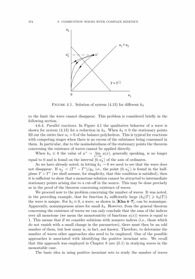
374 9. COMBUSTION WAVES WITH COMPLEX KINETICS
u2−
u2
u−
0 u1
T = T ∗
u1 = u2
Figure 4.1. Solution of system (4.13) for different k3
to the limit the wave cannot disappear. This problem is considered briefly in thefollowing section.
4.6.4. Parallel reactions. In Figure 4.1 the qualitative behavior of a wave isshown for system (4.13) for a reduction in k3. When k3 ≡ 0 the stationary pointsfill out the entire face u1 = 0 of the balance polyhedron. This is typical for reactionswith competing stages when there is no excess of the substance being consumed inthem. In particular, due to the nonisolatedness of the stationary points the theoremconcerning the existence of waves cannot be applied directly.
When k3 ≡ 0 the value of u+ = limx→∞
u(x), generally speaking, is no longer
equal to 0 and is found on the interval [0, u−2 ] of the axis of ordinates.As we have already noted, in letting k3 → 0 we need to see that the wave does
not disappear. If u−2 < (T+ − T ∗)/q3, i.e., the point (0, u−2 ) is found in the half-plane T > T ∗ (we shall assume, for simplicity, that this condition is satisfied), thenit is sufficient to show that a monotone solution cannot be attracted to intermediatestationary points arising due to a cut-off in the source. This may be done preciselyas in the proof of the theorem concerning existence of waves.
We proceed now to the problem concerning the number of waves. It was noted,in the preceding example, that for function k3 sufficiently large (k3(T ) k2(T ))the wave is unique. For k3 ≡ 0, a wave, as shown in [Kha 4–7], can be nonunique.Apparently, nonuniqueness arises for small k3. However, from the general theoremconcerning the existence of waves we can only conclude that the sum of the indicesover all monotone (we mean the monotonicity of functions u(x)) waves is equal to1. This means that if we consider solutions with nonzero indices (i.e., those whichdo not vanish with a small change in the parameters), there must then be an oddnumber of them, but how many is, in fact, not known. Therefore, to determine thenumber of waves other approaches also need to be employed. One of the possibleapproaches is associated with identifying the positive invariant sets. We recallthat this approach was employed in Chapter 8 (see §5.1) in studying waves in themonostable case.
The basic idea in using positive invariant sets to study the number of waves
BIBLIOGRAPHIC COMMENTARIES 375
consists in the following. First, we need to determine the conditions for which thereis more than one positive invariant set in the balance polyhedron; in particular,conditions such that a wave cannot belong simultaneously to two sets. And, second,we need to show that a wave exists in each invariant set. This approach can berealized for the reactions (4.8) and for more involved examples.
Bibliographic commentaries1
Earlier in this chapter the proof for the existence of waves in combustionproblems was carried out by the Leray-Schauder method (see [Vol 6, 22–25]).There are many papers in which the existence of combustion waves is proved byother methods. We turn our attention briefly to some of these papers, changingthe notation whenever necessary.
One of the first papers in which a proof for the existence of combustion waveswas given is a paper by Ya. I. Kanel′ [Kan 4]. In it he considered the system ofequations
(C.1)u′′ − cu′ + f(u)v = 0,
λv′′ − cv′ − f(u)v = 0,
with boundary conditions
(C.2) u(±∞) = u±, v(−∞) = v− > 0, v(+∞) = 0.
Here u and v are, respectively, dimensionless temperature and concentration of theinitial substance; c is the wavespeed; λ is the ratio of the coefficient of diffusionto the coefficient of heat conduction; f(u) = 0 for u < α, f(u) > 0 for u > α,u− < α < u+.
Setting p = u′ and considering u as an independent variable, from (C.1) weobtain
(C.3)
dp
du= c− f(u)v
p,
dv
du=c
λp(u+ v − u+)−
1λ.
Instead of boundary conditions (C.2), the conditions specified are
(C.4) v(u−) = v−, v(u+) = 0, p(u±) = 0.
The solution p(u) of system (C.3) may be estimated from above and from below bythe solutions p1(u) and p2(u) of the equations
dp
du= c− f(u)u+ − u
p
anddp
du= c− f(u)u+ − u
λp
and, with the aid of these estimates, existence of solutions of problem (C.3), (C.4)is established. Moreover, if 0 < λ < 1, uniqueness of the solution is also proved.In [Beres 4] a proof is also given for the existence of solutions for system (C.1) and
1 See also the supplement to Part III.
376 9. COMBUSTION WAVES WITH COMPLEX KINETICS
asymptotic solutions are obtained for the case in which the activation energy tendstowards infinity.
A problem of interest is that concerning the number of waves for λ > 1.This problem was considered in [Bac 1] for the case in which the coefficients ofdiffusion and heat conduction depend on the temperature. In this case the systemof equations has the form
(α1(u)u′)′ − cu′ + f(u)v = 0,
(α2(u)v′)′ − cv′ + f(u)v = 0,
where α2(u)/α1(u) ≡ λ. By methods similar to those used in [Kan 4] it was shownthat for arbitrary λ > 1 the function ϕ(u) = α1(u)f(u) can be selected so that atleast two waves exist. Nonuniqueness of combustion waves is shown also in [Bon 2].
As has already been noted, nonuniqueness can have a kinetic nature. This wasfirst proved in [Kha 4–7] for the case of parallel reactions by a method of matchingof asymptotic expansions (see also §4 and the supplement to Part III).
There are many papers in which existence of waves is proved on the basis of ananalysis of the behavior of trajectories in the phase space of an autonomous systemof first order equations: in [Vag 1] for the propagation of a combustion wave in acondensed medium; in [Shk 2] in the presence of heat loss for a reaction of zeroorder; in [Vol 33] for polymerization and crystallization that, in essence, are closeto sequential reactions; in [Kis 1] for the case of more complex kinetics.
In [Beres 1, Bon 1, Hei 1] the Leray-Schauder method is applied in provingthe existence of combustion waves with a complex kinetics. This method is appliedin proving the existence of solutions on a finite interval, following which a passageto the limit is made over the length of the interval.
Problems relating to the stabilization of solutions of equations from combustiontheory were studied in [Kan 5]. Finally, we note also the papers [Beres 2–4,Braun 1, 3, Gio 1, Has 5, Nor 1, 2] in which various problems of combustion areconsidered.
CHAPTER 10
Estimates and Asymptoticsof the Speed of Combustion Waves
The speed of combustion waves is an important characteristic of these waves.A large number of papers devoted to a study of this characteristic exist, mainly,by approximate analytical and asymptotic methods (see the commentaries to thischapter and the supplement to Part III). Here, as a rule, a question arises about theaccuracy of the results obtained and the domain of their applicability. Therefore,in many cases analytical investigations are supplemented by numerical studies. Inthis chapter the speed of combustion waves is investigated by the minimax methodand by the method of successive approximations, a method very little employedfor the study of wave solutions of parabolic equations. This situation is apparentlyassociated with the fact that the mathematical theory has not been sufficientlydeveloped; moreover, in using these methods certain technical difficulties can arise,the sense of which will be made clear below.
A minimax representation for the wavespeed was obtained in Chapter 1 fora scalar equation and in Chapter 5 for monotone systems of equations describinga broad class of gas combustion processes (see Chapters 8, 9). In this chapter aminimax representation for the speed will also be obtained for a model of gaslesscombustion. The minimax method makes it possible to obtain two-sided estimatesof the speed, the accuracy of which is determined by the proximity of estimates fromabove and from below. If the asymptotics of the estimates from above and frombelow are in agreement, then asymptotics of the speed will have been obtained.In §1 the minimax method is applied to the analysis of several models of gaslesscombustion; in §2 combustion of gases is considered.
The method of successive approximations (§3) also makes it possible to obtaintwo-sided estimates and asymptotics of the speed. Its application to combustionproblems is illustrated for a model describing propagation of a combustion wave ina condensed medium. We remark that the basic test-function used in the minimaxmethod in some cases serves as an accurate first approximation in the successiveapproximations method.
§1. Estimates for the speed of a combustion wave in a condensed medium
1.1. Introduction. We consider the system of equations
κd2T
dx2− v dT
dx+ qϕ(a)k(T ) = 0,(1.1)
vda
dx+ ϕ(a)k(T ) = 0,(1.2)
describing propagation of the combustion front in a condensed medium during the377
378 10. ESTIMATES AND ASYMPTOTICS OF THE SPEED OF COMBUSTION WAVES
course of a single-stage chemical reaction. Here T and a are the temperature andconcentration of a reactant, v is the speed of the front, x is a spatial variable,−∞< x <∞, ϕ(a) gives the kinetics of the reaction, κ is the coefficient of thermaldiffusivity, q = Q/c, where Q is the thermal effect of the reaction and c is the heatcapacity. The reaction rate has an Arrhenius temperature dependence
k(T ) = k0 exp(−E/RT ) (Tc < T ),
k(T ) = 0 (Ti < T < Tc),
where Tc is the cut-off temperature, k0 is a pre-exponential factor, E is theactivation energy, and R is the gas constant. Boundary conditions in domainsof the cold reactant (x → −∞) and of the reaction products (x → +∞) have theform
x→ −∞ : T = Ti, a = 1; x→ +∞ : dT/dx = 0,
where Ti is the initial temperature of the reactant.It is well known that equations (1.1)–(1.2) can be reduced to a single equation
for the concentration as a function of the temperature
da
dT=
κ
v2ϕ(a)k(T )T − Tb + qa
,(1.3)
T = Tc : a = 1; T = Tb : a = 0,(1.4)
where Tb is the combustion temperature, Tb = Ti + q.Equation (1.3) can, in turn, be written in the form
(1.5) v2 = B(a(T ), T ),
where
(1.6) B(ρ(T ), T ) =κϕ(ρ)k(T )
(T − Tb + qρ)dρ/dT.
In case a(T ) is a solution of problem (1.3)–(1.4) the right-hand side of (1.5),considered as a function of T , is a constant, equal to v2. We take an arbitraryfunction ρ(T ) satisfying the same boundary conditions (1.4). Expression (1.6) isthen no longer a constant and the essence of the method being described consistsin the fact that the minimal and maximal values of the function B(ρ(T ), T ) yieldestimates of v2 from below and from above, respectively. We remark that functionρ(T ) can be chosen in an arbitrary way and an arbitrary test function allows usto obtain the estimates. Nevertheless, the closer the test function is to the exactsolution, the better are the estimates obtained, and conversely, the accuracy of theestimates obtained indicates the proximity of the test function to the exact solution.Thus we are in a position to clarify the accuracy of approximate solutions knownin the literature.
§1. SPEED OF CONDENSED PHASE COMBUSTION 379
As a simple example of an application of this approach we obtain estimates ofthe speed for a first order reaction (ϕ(a) = a):
(1.7) σ < v2 <σ
1− σ/(κk(Tb)),
where
σ = κ
∫ Tb
Tc
k(T ) dTT − Ti
.
In order to analyze these estimates, we note that for large activation energiesthe integral in (1.7) can be calculated approximately by means of the Frank-Kamenetskiı transform [Fran 1]
∫ Tb
Tc
k(T ) dTT − Ti
≈ RT 2b k(Tb)
E(Tb − Ti).
Thus, from (1.7) it follows that
κk(Tb)RT 2
b
Eq< v2 < κk(Tb)
RT 2b
Eq/
[1− RT
2b
Eq
].
As a rule, the quantity RT 2b /Eq is of order 0.1, and thus we can find a value for
the speed accurate to within several percent.A second example relates to heterogeneous combustion with wide reaction
zones, usually modeled by means of exponential kinetics
ϕ(ρ) = exp[−m(1− ρ)] (ρ > 0),
ϕ(ρ) = 0 (ρ 0).
In this case,
σ1 < v2 < eσ1 (e ≈ 2.71),
where
σ1 = κk0m exp[1− 2
(Em
Rq
)1/2
+mTiq
].
The content of this section is as follows. In §1.2 we give a precise formulationof the minimax approach and a short proof of it. Two-sided estimates of the speedfor an nth order reaction are derived in §1.3. In §1.4 some generalizations of theapproaches used are considered for the case of a reaction of arbitrary kinetics.Exponential kinetics, in the case of large m, is considered in §1.5.
380 10. ESTIMATES AND ASYMPTOTICS OF THE SPEED OF COMBUSTION WAVES
1.2. Variational approach. We introduce the following dimensionless vari-ables and parameters:
θ = (T − Tb)/q; γ = RT 2b /(qE); β = RTb/E;
h = (Tc − Ti)/q, δ = β/γ, u = v/[κγk0 exp(−1/β)]1/2.
Problem (1.3)–(1.4) then takes the form
(1.8)da
dθ= − 1
γu2ϕ(a)Φ(θ)a+ θ
,
where the initial temperature is θi = −1, θc = −1 + h; the burning temperature isequal to 0, and the boundary conditions may be written as
(1.9) a(θc) = 1, a(0) = 0.
Here
Φ(θ) = exp[θ/(γ + βθ)] (θc θ 0),
Φ(θ) = 0 (θi θ < θc).
We denote by Ω1 the set of smooth, monotonically decreasing functions ρ(θ),defined on [θc, 0] and satisfying the boundary conditions
ρ(θc) = 1, ρ(0) 0.
We consider also the set of smooth, monotonically decreasing functions ρ(θ), definedon [θc, θ∗] for arbitrary θ∗, θc < θ∗ 0, and satisfying the boundary conditions
ρ(θc) = 1, ρ(θ∗) = −θ∗.
We denote this set of functions by Ω2.
Theorem 1.1. Let Ω1 and Ω2 be the sets of functions described above. Then
(1.10) u2 = infρ∈Ω1
maxθcθ0
B(ρ(θ), θ) = supρ∈Ω2
minθcθθ∗
B(ρ(θ), θ),
where
(1.11) B(ρ(θ), θ) ≡ − 1γ
ϕ(ρ)Φ(θ)(ρ+ θ)dρ/dθ
.
From (1.10) we have the following inequalities for arbitrary ρ1 ∈ Ω1, ρ2 ∈ Ω2:
(1.12) minθcθθ∗
B(ρ2(θ), θ) u2 maxθcθ0
B(ρ1(θ), θ).
These inequalities play an important role later on in a derivation of estimates ofthe speed. Moreover, (1.10) follows from (1.12) since there exists a test function—namely, the exact solution—for which (1.10) is satisfied. Thus it is sufficient toprove (1.12).
§1. SPEED OF CONDENSED PHASE COMBUSTION 381
Proof. Suppose that the inequality on the right-hand side of (1.12) does nothold. Then there exists a function ρ1 ∈ Ω1 such that
u2 > B(ρ1(θ), θ)
and such that, for arbitrary θ,
dρ1dθ
< − 1γu2
ϕ(ρ1)Φ(θ)ρ1(θ) + θ
.
Therefore, if trajectory ρ(θ) of equation (1.8) intersects the graph of the testfunction at a point θ ∈ [θc, 0), i.e., a(θ) = ρ1(θ), then
da/dθ|θ=eθ > dρ1/dθ|θ=eθ.
Since this inequality is also satisfied for θ = θc, we have a(θ) > ρ(θ) for arbitraryθ ∈ (θ, 0]. If ρ1(0) > 0, then a(0) > 0 and we obtain a contradiction with boundaryconditions (1.9). In case ρ1(0) = 0, there exists a whole family of trajectories cominginto the point (0, 0), which contradicts the saddle-type nature of this point.
The inequality on the left side of (1.12) is proved similarly.
Remark. The statement of the theorem remains valid even in the cases of areaction of zero order and of exponential kinetics, although here the point (0, 0) isnot even a stationary point.
1.3. Estimates of the speed of the front for an nth order reaction. Inthis section we assume that ϕ(a) = an. We first consider the case of a reaction ofthe first order (n = 1). As a test function we take
(1.13) ρ(θ) = 1− J(θ)/J(0),
where
(1.14) J(θ) =∫ θ
θc
Φ(θ) dθγ(1 + θ)
.
It is easy to see that ρ(θ) is a smooth, monotonically decreasing function satisfyingthe boundary conditions (1.9). Thus this function can be used both for obtainingestimates from above and for obtaining estimates from below.
Substituting (1.13), (1.14) into (1.11), we obtain the following expression:
(1.15) B(ρ(θ), θ) = J(0)ρ(θ)(1 + θ)ρ(θ) + θ
,
for which maximal and minimal values must be found. We show that these valuesare J(0) and J(0)/[1− γJ(0)], respectively, assuming, for simplicity, that
(1.16) h > (1− δ)/δ.
This condition is not a necessary condition; nevertheless, since it is satisfied forparameter values typical for combustion, we shall require its fulfillment.
Lemma 1.1. Suppose that condition (1.16) is satisfied. Then function ξ(θ),defined by the expression
ξ(θ) = γJ(θ) exp[− θ
γ(1 + δθ)
],
is a monotonically increasing function of θ.
382 10. ESTIMATES AND ASYMPTOTICS OF THE SPEED OF COMBUSTION WAVES
Proof. It is easy to see that the equation
ξ′(θ) = 0
is equivalent to
ξ(θ) = R(θ),
where
R(θ) = γ(1 + δθ)2/(1 + θ).
From (1.16) it follows that R(θ) is a monotonically increasing function for θ ∈ (θc, 0),and we show that
(1.17) ξ(θ) < R(θ)
for arbitrary θ ∈ (θc, 0). If (1.17) is not satisfied, then there exists a value θ, suchthat ξ(θ)<R(θ) for θ ∈ (θc, θ) and ξ(θ) =R(θ) (i.e., ξ′(θ) = 0), since ξ(θc)<R(θc).Thus we have ξ′(θ) = 0, R′(θ) > 0, and, consequently, in contradiction with (1.17),ξ(θ) > R(θ) for θ less than θ but sufficiently close to it. By virtue of (1.17),ξ′(θ) > 0.
Lemma 1.2. Suppose (1.16) is satisfied. Then for γ < 1
ξ(θ) < 1 (θc θ 0).
Proof. It follows from the proof of Lemma 1.1 that for arbitrary θ ∈ [θc, 0]
ξ(θ) R(θ) R(0) = γ < 1.
Lemma 1.3. Assume ξ(θ) < 1 for arbitrary θ ∈ [θc, 0]. Then
(1.18) ρ(θ) + θ > 0 (θc θ < 0).
Proof. Inequality (1.18) is equivalent to
(1.19) q(θ) ≡ J(θ)/(1 + θ) < J(0) (θc θ < 0).
It is easy to see that q(θc) = 0, q(0) = J(0). In addition, q(θ) is a monotonicallyincreasing function since
q′(θ) =1− ξ(θ)γ(1 + θ)2
expθ
γ(1 + δθ)> 0,
and, consequently, (1.19) is satisfied.
We proceed now to the proof of the main result for the case of a first orderreaction.
§1. SPEED OF CONDENSED PHASE COMBUSTION 383
Theorem 1.2. Let u be the speed of propagation of the combustion wave inproblem (1.8)–(1.9), where ϕ(a) = a. We assume that condition (1.16) is satisfiedand that γ < 1. Then
(1.20) J(0) < u2 < J(0)/[1− γJ(0)].
Proof. We show that for arbitrary θ ∈ [θc, 0]
J(0) = B(ρ(θc), θc) B(ρ(θ), θ) B(ρ(0), 0) = J(0)/[1− γJ(0)].It follows from Lemma 1.3 that B(ρ(θ), θ) is a smooth function. Then
B(ρ(θ), θ) = J(0) + J(0)(−θ)(1 − ρ)ρ+ θ
J(0)
and the inequality on the left in (1.20) is established.In fact, under the assumptions made, B(ρ(θ), θ) is a monotonically increasing
function; however, we confine the discussion to proving that if B(ρ(θ), θ) has amaximum at point θm, then
B(ρ(θm), θm) B(ρ(0), 0).The equation B′(ρ(θ), θ) = 0 is equivalent to θm = −ξ(θm)ρ(θm). Consequently,
(1.21) B(ρ(θm), θm) = J(0)ρ(θm)(1 + θm)ρ(θm) + θm
= J(0)1 + θm
1− ξ(θm).
Since ξ(θ) is a monotonically increasing function, we have
0 ξ(θ) γJ(0)and (1.20) then follows from (1.21). This completes the proof of the theorem.
We consider the case 0 n 1 and take the test function in the form
(1.22) ρ(θ) = [1− J(θ)/J(0)]1/(2−n).
As above, ρ(θ) is a monotonically decreasing function satisfying the boundaryconditions (1.9). Substituting (1.22) into (1.11), we obtain
B(ρ(θ), θ) = (2− n)J(0)(1 + θ)/[1 + θ/(1− J(θ)/J(0))]1/(2−n).
It is easy to see that the denominator of the right-hand side is a monotonicallydecreasing function of n for arbitrary fixed θ. Then
B(ρ(θ), θ) (2− n)J(0)(1 + θ)/[1 + θ/(1− J(θ)/J(0))] (2− n)J(0)/[1− γJ(0)]
as in the case of a reaction of the first order. Further,
B(ρ(θ), θ) = (2− n)J(0)[1 + (−θ)(1 − ρ)/(ρ+ θ)] (2− n)J(0).
A result of our considerations is the following theorem.
Theorem 1.3. Let u be the speed of the wave in problem (1.8)–(1.9). Let usassume that 0 n 1, γ < 1, and that (1.16) is satisfied. Then
(2− n)J(0) < u2 < (2− n)J(0)/[1− γJ(0)].
We proceed now to estimate the speed of the combustion wave in the case1 < n 3.
384 10. ESTIMATES AND ASYMPTOTICS OF THE SPEED OF COMBUSTION WAVES
The test function is taken in the form
(1.23)ρ2−n(θ) = 1 +
n− 2σJ(θ) (n = 2),
ρ(θ) = exp[− 1σJ(θ)
](n = 2).
Parameter σ will be selected later. We note, in the case n > 1, that σ is selecteddifferently when obtaining estimates from above and from below.
Substituting (1.23) into (1.11), we obtain
(1.24) B(ρ(θ), θ) = σρ(θ)(1 + θ)ρ(θ) + θ
.
In deriving estimates from above, the denominator in (1.24) must be positive. Thiscondition can be written as
σ > F (θ) (θc θ < 0),
where
F (θ) =(2− n)J(θ)1− (−θ)2−n (n = 2),
F (θ) = −J(θ)/ ln(−θ) (n = 2).
The simplest method of obtaining estimates from below consists in the follow-ing. Let θm be the maximum point of function F (θ). We set
(1.25) σ = F (θm).
Then
1 ρ(θ) > −θ (θc θ < θm),ρ(θm) = −θm,
and we can use the minimax approach to obtain estimates of the speed from below.Taking into account (1.25) and the inequality
(1.26) B(ρ(θ), θ) = σρ(θ)(1 + θ)1 + θ/ρ(θ)
σ (θc θ 0)
we obtainu2 min
θcθθm
B(ρ(θ), θ) σ F (θ) (θc θ 0).
Thus, each value of function F (θ), θc θ 0, can be considered as an estimatefrom below for u2:
u2 (2 − n)J(0)/[1− (−θ)2−n].
When n 1.5, we can take θ = 0, which gives u2 (2 − n)J(0). In case n > 1.5,it is better to take
θ = −(γ
2− n1− γ2−n
)1/(n−1)
.
To obtain estimates of the speed of propagation from above, we must findthe maximum value of B(ρ(θ), θ). As a rule, this problem becomes involved whenseeking an analytic solution. It could be solved numerically, but our principal aimhere is to obtain analytical estimates. We proceed by obtaining estimates from
§1. SPEED OF CONDENSED PHASE COMBUSTION 385
above for the maximum value of function B. The main idea consists in obtainingestimates of ρ(θ) from below and obtaining, thereby, a new function instead of B,one which we can study analytically.
Lemma 1.4. Let condition (1.16) be satisfied. Then for an arbitrary root θr ofthe equation
(1.27)dB(ρ(θ), θ)
dθ= 0
we have the inequality
(1.28) −γ < θr,
proving that γ < 1, n 3.
Proof. Equation (1.27) can be written in the form
θ + ξ(θ)(2 − n) ρ2−n
1− ρ2−n (1− ρ) = 0.
It is easy to see that for 0 n 3, 0 τ 1, we have the inequality
(1.29) 0 (2− n) τ2−n
1− τ2−n (1 − τ) 1.
From (1.29) it follows that all solutions of equation (1.27) lie in the interval (θ1, 0),where θ1 is the solution of the equation
θ + ξ(θ) = 0.
Since ξ(θ) γ for θ arbitrary, θc θ 0, then θ1 > −γ and the lemma is therebyproved.
Remark. The same result (1.28) holds for solutions of the equation
F ′(θ) = 0,
since it can also be written in the form
θ + ξ(θ)(2 − n) (−θ)2−n1− (−θ)2−n (1 + θ) = 0.
Lemma 1.5. Let condition (1.16) be satisfied, 0 n 3, and let γ < 1. Thenfor −γ θ 0
(1.30) J(θ) J(0)[bθ + 1],
whereb = (1− p)/γ, p = J(−γ)/J(0).
Proof. It is sufficient to show that J ′′(θ) > 0. We have
J ′′(θ) =1− γR(θ)
γ2(1 + θ)(1 + δθ2)exp
θ
γ(1 + δθ)> 0,
since γR(θ) < γR(0) = γ < 1. On the right-hand side of (1.30) a straight line joins
386 10. ESTIMATES AND ASYMPTOTICS OF THE SPEED OF COMBUSTION WAVES
the two points (0, J(0)) and (−γ, J(−γ)), so that (1.30) is satisfied by virtue of theconvexity of J(θ).
Lemma 1.6. Suppose that (1.16) is satisfied and that γ < 0.45. Then
γ < 1− 2p.
Proof. It is easy to see that for δ 0.5
(1.31) p =J(−γ)J(0)
=ξ(−γ)ξ(0)
exp[− 1
1− δγ
] exp
[− 1
1− γ/2
],
and that the inequality
γ + 2 exp[− 1
1− γ/2
]< 1
is satisfied for the indicated values of γ.
Theorem 1.4. Let u be the speed of propagation of the combustion wave inproblem (1.8)–(1.9). Let us assume that 1 n 3, γ < 0.45, and that (1.16) issatisfied. Then
u2 (2− n)J(0)1− (0.64γ)2−n
.
Proof. Since the maximum of B(ρ(θ), θ) occurs on the interval (−γ, 0), wehave
(1.32)u2 max
θcθ0B(ρ(θ), θ) = max
−γθ0σ
1 + θ1 + θ/ρ
max−γθ0
σ
1 + θ/[1 + (n− 2)σ−1J(0)(bθ + 1)]1/(2−n)
if σ is such that the denominators of the fractions in (1.32) are positive for all θ,−γ θ 0. Let us set
σ =(2− n)J(0)
1− (n− 1)bn−2.
Then σ is positive for 1 n 3 if γ < 2− 2p. This condition is satisfied by virtueof Lemma 1.6. To prove positivity of the denominators it is sufficient to show thatthe last of them in (1.32) is positive. We denote it by f(θ). Then
f(θ) = 1 +θ
[−bθ + (n− 1)bn−2(bθ + 1)]1/(2−n).
It is easy to see that f(0) = 1, f ′(0) = 1, and that f(θ) has only one minimum at
θM =(n− 2)bn−3
1− (n− 1)bn−2
and
f(θM ) =1− bn−2
1− (n− 1)bn−2.
Since γ < 2 − 2p, then f(θM ) > 0, and it follows from Lemma 1.2 that θM > −γfor γ < 0.45. Thus
max−γθ0
σ
f(θ)=
(2− n)J(0)1− bn−2
§1. SPEED OF CONDENSED PHASE COMBUSTION 387
and
u2 (2− n)J(0)1− [(1 − p)/γ]n−2
(2− n)J(0)1− (0.64γ)2−n
by virtue of (1.31). This completes the proof of the theorem.
Remark 1. In case 0.45 < γ < 1 we can set
σ = J(0)[1− (n− 1)p]
and, following similar arguments, we obtain
u2 J(0)[1 − (n− 1)p]1− γ[(1− p(n− 1))/(1− p)]1/(n−2)
.
Remark 2. The above analysis allows us to present an approximate formulafor the speed of the combustion wave:
u2 =(2 − n)J(0)1− γ2−n (0 n 3).
1.4. Arbitrary kinetic laws. We proceed now to estimate the speed of acombustion wave in the case of arbitrary kinetic laws. In fact, we could alsoconsider arbitrary temperature dependences; nevertheless, for simplicity we confinethe discussion to Arrhenius dependence. Thus we consider problem (1.8)–(1.9)with the function Φ(θ) defined above, and an arbitrary function ϕ(a) satisfying theconditions
ϕ(0) = 0, ϕ(1) = 1
(certain other restrictions will be indicated later).As was done above, for the test function we take a solution of the equation
(1.33)dρ
dθ= − 1
γσ
ϕ(ρ)Φ(θ)/ρ1 + θ
.
Let
Ψ(ρ) =∫ 1
ρ
ξ dξ
ϕ(ξ).
Then, integrating (1.33), we obtain
Ψ(ρ) = J(θ)/σ.
Here the boundary condition ρ(θc) = 1 is satisfied. For simplicity, we shall assumethat Ψ(0) <∞. We set
σ = J(0)/Ψ(0).
Then ρ(θ) is a solution of the equation
(1.34) J(0)/Ψ(0) = J(θ)/Ψ(ρ).
Since ρ(0) = 0, the test function is appropriate for obtaining estimates, both
388 10. ESTIMATES AND ASYMPTOTICS OF THE SPEED OF COMBUSTION WAVES
from above and from below. Substituting ρ(θ) into (1.11), we obtain (1.24). Thecondition for positivity of the denominator in (1.24) can be written in the form
(1.35) J(0)/Ψ(0) > J(θ)/Ψ(−θ) (θc < θ < 0).
From this, as we did above, we can conclude that
B(ρ(θ), θ) σ
and, consequently,u2 J(0)/Ψ(0).
To obtain estimates from above, we estimate the roots of the equation
(1.36) dB(ρ(θ), θ)/dθ = 0,
and also function ρ(θ) in (1.24) by means of a linear function on this interval. Theexpression obtained thereby can be readily studied.
Equation (1.36) can be rewritten in the form
−θm = g(ρ)ξ(θm),
where
g(ρ) ≡ ρ2(1 − ρ)ϕ(ρ)Ψ(ρ)
.
Let
(1.37) gm = max0ρ1
g(ρ)
and let us assume that condition (1.16) is satisfied. Then
θm > −γgm
(compare with Lemma 1.4). As was the case above, the points at which the functionon the right-hand side of (1.35) attains maxima are also situated on the interval(−γgm, 0). Thus, positiveness of the denominator of B follows from the estimatespresented below. Since J ′′(θ) > 0, we have
J(θ)J(0)
1− θ
θ1
[1− J(θ1)
J(0)
](θ1 θ 0),
whereθ1 = −γgm.
Taking (1.34) into account, we obtain
Ψ(ρ)Ψ(0)
1− θ
θ1
[1− J(θ1)
J(0)
](θ1 θ 0)
and, consequently,
−θ 1k
(1− Ψ(ρ)
Ψ(0)
)(θ1 θ 0),
wherek = −[1− J(θ1)/J(0)]/θ1.
§1. SPEED OF CONDENSED PHASE COMBUSTION 389
Thus,
u2 maxθcθ0
σρ
ρ+ θ= maxθ1θ0
σ1
1 + θ/ρ
max0ρ1
σ
1− [1−Ψ(ρ)/Ψ(0)]/(kρ).
Let
(1.38) pm = max0ρ1
p(ρ), p(ρ) = [1−Ψ(ρ)/Ψ(0)]/ρ.
Then
u2 σ
1− γgmpm/[1− J(θ1)/J(0)] σ
1− γgmpm/[1− exp(−gm)].
As a result of these considerations, we have the following theorem.
Theorem 1.5. Let u be the speed of the combustion wave in problem (1.8)–(1.9) with the arbitrary kinetics ϕ(a) satisfying the conditions formulated above.Let us assume that (1.16) is satisfied and that
γ < min[1− exp(−gm)
gmpm, 1],
where gm, pm are given by formulas (1.37), (1.38). Then
(1.39)J(0)Ψ(0)
u2 J(0)/Ψ(0)1− γgmpm/[1− exp(−gm)]
.
For γ sufficiently small, (1.39) gives an accurate approximation for the propa-gation velocity.
We apply the results obtained to the case of exponential kinetics:
ϕ(a) = exp[−m(1− a)] (a > 0),
ϕ(a) = 0 (a < 0).
We have
(1.40)
Ψ(ρ) = [(1 +mρ) exp(m(1 − ρ))− (1 +m)]/m2,
g(ρ) = m2 ρ2(1 − ρ)(1 +mρ)− (1 +m) exp[−m(1− ρ)] ,
p(ρ) =1− (1 +mρ) exp(−mρ)[1− (m+ 1) exp(−m)]ρ
,
and the problem consists in finding gm and pm.
390 10. ESTIMATES AND ASYMPTOTICS OF THE SPEED OF COMBUSTION WAVES
Lemma 1.7. If m 3, then gm = 1. For m > 3
gm Am = (3 +m)2/(4m)− 2.
Proof. Inequality g(ρ) 1 is equivalent to
(1.41) r(x) 1,
where
x = 1− ρ, r(x) =[1−mx+ 2m2x2
1 +m− m2x3
1 +m
]exp(mx).
Since r(0) = 1, r′(x) 0 for 0 x 1, m 3, formula (1.41) is satisfied. Considerthe case m > 3. We have g(0) = 0, g(1) = 1, and from
g′(ρ∗) = 0
it follows that
(1.42) (1 +m) exp[−m(1− ρ∗)] =2mρ2∗ + (3 −m)ρ∗ − 2−mρ2∗ + (3 +m)ρ∗ − 2
.
Substituting (1.42) into (1.40), we obtain
g(ρ∗) = −mρ2∗ + (3 +m)ρ∗ − 2 Am.
Lemma 1.8. Let x∗ be a positive solution of the equation
expx = x2 + x+ 1
(x∗ ≈ 1.793). Then
pm = 1 (m x∗),
pm = mζ(x∗)/[1− (m+ 1) exp(−m)] (m > x∗),
whereζ(x) = [1 − (1 + x) exp(−x)]/x.
Proof. Function p(ρ) can be written in the form
p(ρ) = mζ(mρ)/[1 − (m+ 1) exp(−m)].
Consequently,pm = max
0mρmζ(mρ)m/[1− (m+ 1) exp(−m)].
It is easy to see that function ζ(x) increases monotonically for x < x∗ anddecreases for x > x∗. Consequently,
max0mρm
ζ(mρ) = ζ(m) (m < x∗),
max0mρm
ζ(mρ) = mζ(x∗)/[1− (m+ 1) exp(−m)] (m > x∗),
and the lemma is proved (ζ(x∗) = 0.298).
§1. SPEED OF CONDENSED PHASE COMBUSTION 391
As a result, we have
(1.43)m2J(0)
exp(m)− (m+ 1) u2 m2J(0)
exp(m)− (m+ 1)1
1− γcm,
where
cm = e/(e− 1) ≈ 1.582 (m < x∗),
cm = 1.582mζ(x∗)/[1− (m+ 1) exp(−m)] (x∗ m 3),
cm = Ammζ(x∗)/[1− (m+ 1) exp(−m)]/[1− exp(−Am)] (m > 3).
In particular,
c1 ≈ 1.582, c2 ≈ 1.587, c3 ≈ 1.766, c4 ≈ 2.130, c10 ≈ 7.438.
The larger the value of m, the less accurate the estimates (1.43) turn out to be.This is connected with the fact that the test function constructed above is designedfor a narrow reaction zone. For large m the reaction zone becomes wide, a case tobe examined in the next section.
1.5. Estimates of the speed of a combustion wave for exponentialkinetics. In this case it is convenient to use the following dimensionless variablesand parameters:
θ = (T − T∗)/q, γ = (RT 2∗ )/(Eq), δ = q/T∗, θi = (Ti − T∗)/q,
θc = (Tc − T∗)/q, θb = (Tb − T∗)/q, h = θc − θi,
u = v[mκk0 exp(−m+mθb − E/RT∗)]−1/2.
The scaling temperature T∗ is specified by the equation m = RT 2∗ /Eq. Then (1.3)–
(1.4) may be written in the form
da
dθ= − 1
u2exp[ma−mθb +mθ/(1 + δθ)]
ma−mθb +mθ,
a(θc) = 1, a(θb) = 0.
To obtain estimates from above, we take as test function the solution of theequation
dρ
dθ= − 1
σ
exp[m(ρ+ θ − θb)]m(ρ+ θ − θb)
,(1.44)
ρ(θc) = 1, ρ(θb) = 0.(1.45)
Parameter σ must also be found from (1.44)–(1.45). It is easy to show that σ < e.Indeed, let
y(θ) = ρ(θ) + θ − θb.
Then (1.44)–(1.45) takes the form
(1.46)dy
dθ= 1− 1
σ
exp(my)my
,
y(θc) = h, y(θb) = 0.
392 10. ESTIMATES AND ASYMPTOTICS OF THE SPEED OF COMBUSTION WAVES
Integrating (1.46) from θc to θb, we obtain
(1.47) σ
∫ mh
0
xdx
exp(x)− σx = m(1− h).
For simplicity, we shall assume that mh > 1. It then follows from (1.47) that σ < e.In the opposite case the integral in (1.47) does not exist. In fact, for m large, σcan be found more precisely. Without going into the details, we give the result:
σ ≈ e[1− 2π2/m2(1 − h)2] (m# 1).
Substituting ρ(θ) specified by (1.44), (1.45) into B(ρ(θ), θ), we obtain
B(ρ(θ), θ) ≡ −exp[mρ−mθb +mθ/(1 + δθ)]m(ρ+ θ − θb)dρ/dθ
= σ exp[− mδθ2
1 + δθ
] σ e.
Consequently, u2 e, and in dimensional form we have
v2 κmk0 exp[1− 2
(EmRq
)1/2+mTi/q
].
To obtain estimates from below we consider the problem
(1.48)dρ
dθ= − 1
σ
exp[mρ−mθb +mθ/(1 + δθ)]m(ρ− θb)
,
ρ(θc) = 1, ρ(0) = θb.
Obtaining σ from (1.48), we have
σ =∫ 0
θc
exp[−mθb +mθ/(1 + δθ)] dθ/∫ 1
θb
m(ρ− θb) exp(−mρ) dρ
=m∫ 0
θc
exp[mθ/(1 + δθ)] dθ/1− [1 +m(1− θb)] exp[−m(1− θb)].
For m sufficiently large
m
∫ 0
θc
exp[mθ/(1 + δθ)] dθ ≈ 1
andσ ≈ 1
1− [1 +m(1− θb)] exp[−m(1− θb)]> 1.
Substituting ρ defined by (1.48) into B(ρ(θ), θ), we find
B(ρ(θ), θ) = σρ− θb
ρ+ θ − θb> σ > 1.
Thus u2 > 1 and we have, finally,
κmk0 exp[− 2(EmRq
)1/2+mTi/q
] v2 κmk0 exp
[1− 2
(EmRq
)1/2+mTi/q
].
§2. Estimates for the speed of a gas combustion wave
2.1. Minimax method. Test function. In this section we apply the min-imax method for a single-stage nth order reaction in the case of similarity of the
§2. ESTIMATES FOR THE SPEED OF A GAS COMBUSTION WAVE 393
temperature and concentration fields (i.e., for equality of the coefficients of thermaldiffusivity and diffusion).
In coordinates connected with the wave, the stationary system of equations hasthe form
κT ′′ + vT ′ + qank(T ) = 0,(2.1)
da′′ + va′ − ank(T ) = 0,(2.2)
where T is the temperature, a is the concentration of the initial substance; κ and dare the coefficients of thermal diffusivity and diffusion respectively; q is the adiabaticheating of the reaction; n is the order of reaction; v is the wavespeed; and
k(T ) =k0 exp(−E/RT ) (T T∗),0 (Ti T T∗),
E is the activation energy; R is the gas constant; k0 is a pre-exponential factor; Tiis the initial temperature; T∗ is the magnitude of “cut-off” in the source;
x = −∞ : T = Tb ≡ Ti + q, a = 0; x = +∞ : T = Ti, a = 1.
In the case κ = d, as is readily seen, T = Tb − qa and the system of equations(2.1), (2.2) is reduced to a single equation
κT ′′ + vT ′ + q(Tb − Tq
)nk(T ) = 0.
Making variables and parameters dimensionless,
γ =RT 2
b
E(Tb − Ti), β =
RTbE, θ =
T − TbTb − Ti
, k∗ = γk0 exp(−E/RTb),
u = v/√
κk∗, ξ = x√k∗/κ,
we obtain
(2.3) θ′′ + uθ′ + (−θ)nk(θ)/γ = 0.
Here the prime indicates differentiation with respect to ξ,
k(θ) = exp θ
γ+βθ (θ∗ θ 0),
0 (−1 θ < θ∗),θ∗ = (T∗ − Tb)/(Tb − Ti). Conditions at infinity have the form
(2.4) θ(−∞) = 0, θ(+∞) = −1.
We go from equation (2.3) to a system of two first order equations
θ′ = p, p′ = −up− (−θ)nk(θ)/γ,
whence we obtain the equation
(2.5)dp
dθ= −u− (−θ)nk(θ)/(γp)
with boundary conditions
(2.6) p(−1) = p(0) = 0.
394 10. ESTIMATES AND ASYMPTOTICS OF THE SPEED OF COMBUSTION WAVES
We make the change of variablesθ + p/u = −a.
We have
(2.7)da
dθ= − 1
γu2(−θ)nk(θ)a+ θ
, a(θ∗) = 1, a(0) = 0.
We note that this equation resembles that which is obtained for a zero coefficientof diffusion (see §1). The difference is that on the right-hand side of (2.7) we have(−θ)n instead of an.
As we have already remarked several times, selection of a test function doesnot require a formal justification; however, a test function must express the char-acteristic properties of solutions, otherwise the estimates will be poor. In the givencase, in choosing the test function we employ the following considerations. Weconsider equation (2.7) as an equation for d = 0 with a zero order reaction (withrespect to a) and a somewhat modified temperature dependence for the reactionrate. We construct the test function as was done in §1 for a zero order reaction:we rewrite (2.7) in the form
(2.8) ada
dθ= − 1
γu2
(−θ)n exp θγ+βθ
1 + θ/a,
and replace θ/a at the right by θ, assuming that a(θ) is different from 1 only ina narrow interval close to θ = 0; we then solve the resulting equation, using theboundary condition on the left. Thus we obtain the test function
(2.9) ρ(θ) =√1− 2Jn(θ)/σ,
where
(2.10) Jn(θ) =1γ
∫ θ
θ∗
(−τ)n exp τγ+βτ
1 + τdτ
and σ is a parameter whose value is selected for obtaining best estimates.We consider, further, the function
(2.11) B(θ, ρ(θ)) = − 1γ
(−θ)n exp θγ+βθ
(ρ+ θ)dρ/dθ.
Then, by virtue of the minimax method,
(2.12) minθ∗θ0
B(θ, ρ(θ)) u2 maxθ∗θ0
B(θ, ρ(θ)).
We recall that to obtain estimates from above function ρ(θ) must satisfy theconditions
(2.13) ρ(θ) + θ > 0 for θ∗ < θ < 0,
and, for estimates from below,
(2.14) ρ(θ) + θ > 0 for θ∗ < θ < θ0 0, ρ(θ0) = θ0
§2. ESTIMATES FOR THE SPEED OF A GAS COMBUSTION WAVE 395
(if θ0 < 0, then the minimum in (2.12) is taken over the interval θ∗ θ θ0).Substituting (2.9), (2.10) into (2.11), we obtain
(2.15) B(θ, ρ(θ)) = σ(1 + θ)ρθ + ρ
.
We note thatdρ
dθ= − 1
γσ
(−θ)n exp θγ+βθ
(1 + θ)/ρ,
therefore, for σ = 2J(0), ρ(0) = 0 and ρ′(0) = 1/√2J(0)γ for n = 1 and ρ′(0) = 0
for n > 1.
2.2. Estimates of the speed from below. It is easy to see that B σ forθ + ρ > 0. Therefore, setting σ = 2Jn(0), we obtain an estimate from below:
(2.16) u2 2γ
∫ 0
θ∗
(−τ)n exp τγ+βτ
1 + τdτ.
We note that the narrow reaction zone method also yields an estimate of thespeed from below (see [Zel 5, Vag 1]):
u2 > 2Jn =2γ
∫ 0
θ∗
(−τ)n exp τ
γ + βτdτ.
It is easy to see that Jn > Jn, i.e., the estimate (2.16) is more precise than thatobtained by the narrow zone method. Moreover, if for condensed system (d= 0) thedifference between these estimates is small, then, in the case of the combustion ofgases, this difference can be substantial. For example, for γ = 0.1, θ∗ =−0.9, β = 0,and n = 1, we have J1 ≈ 0.13, J1 ≈ 0.10, and for n = 2, J2 ≈ 0.031, J2 ≈ 0.020.Thus, for n = 2 these estimates already differ by a factor of 1.5, whereby, as nincreases, the difference increases. For n = 0 the estimate (2.16) coincides with theestimate for d = 0.
Before presenting yet another estimate from below, we note that to satisfyinequality (2.13) it is obviously sufficient that the following inequality be satisfied:
(2.17) σ >2Jn(θ)1− θ2 ≡ Φ(θ) (θ∗ θ < 0).
If inequality (2.17) is not satisfied, and if for some θ = θ we have the equalityσ = Φ(θ), then the estimate of the speed from below, namely, u2 Φ(θ), followsfrom the inequality B σ. Since σ can be selected arbitrarily, for arbitrary θ thefollowing inequality is obviously satisfied:
u2 2Jn(θ)1− θ2
(cf. §1).
2.3. Estimates from above for 0 n 1. As in the case of a condensedmedium, when n = 1 and with a corresponding choice of σ, the function B(θ, ρ(θ))is a monotone function of θ upon the fulfillment of certain conditions on theparameters of the problem. It attains its smallest value for θ = θ∗ ≡ −1 + h,and its largest value for θ = 0. This makes it possible to calculate its minimum andmaximum explicitly for θ∗ θ 0.
396 10. ESTIMATES AND ASYMPTOTICS OF THE SPEED OF COMBUSTION WAVES
Thus, we consider B(θ, ρ(θ)) as a function of θ for n = 1, σ = 2J1(0). Equatingthe derivative of B to zero, we obtain the equation
F (y) ≡ 2I1(0)[1− I1(y)
I1(0)
][1−
√1− I1(y)
I1(0)
]− y2Φ(y) = 0,
where
I1(y) =
y∫(−1+h)/γ
(−τ)Ψ(τ)1 + γτ
dτ, Ψ(y) = expy
1 + βy, y =
θ
γ.
It is easy to see that F (0) = 0, F ((−1 + h)γ) < 0. Function F will therefore benegative on the half-interval (−1 + h)/γ < y 0 if it is negative at the extremumpoints. From the equation F ′(y) = 0 we obtain
ρ(y) ≡
√1− I1(y)
I1(0)= −2γy
3− y(1 + γy)
3(1 + βy)2.
Substituting into the expression for F (y) the value of ρ(y) found at the extremumpoints, and requiring the resulting function to be negative, we obtain the condition
(2.18)227I1(0)z2(3 + yz)− exp
( y
1 + βy
)< 0,
where(−1 + h)/γ y 0, z = 2γ + (1 + γy)(1 + βy)−2,
upon whose fulfillment function B is monotone. It is easy to see that for γ = 0 thisinequality has the form
2 + 2y/3 < 9ey
and is satisfied for all y (I1(0)→ 1 as γ → 0). We can therefore assume that (2.18)is satisfied also for small γ.
Condition (2.18) is an explicitly verifiable condition on the parameters γ, β,and h, although fairly involved. It can be established analytically under certainconditions; however, it can also be verified numerically. One of the results of anumerical verification is that (2.18) is satisfied in case β = γ < 1. Here we haveused the estimates
I1(0)|h =0 < I1(0)|h=0 = −1γ2
+1γ
(1 +
1γ
)ψ(1γ
) 1 + 2γ
1 + 6γ + 6γ2,
where
ψ(η) = ηeηE1(η), E1(η) =∫ ∞
η
e−tdt
t, ψ(η) η2 + 5η + 2
η2 + 6η + 6
(see [Vol 34, Abr 1]).Thus, under the above conditions on the parameters, we have the estimate
(2.19) 2J1(0) u2 2J1(0)1−√2J1(0)γ
.
Since J1(0) ≈ γ for γ small, the ratio of the estimate from below to the estimatefrom above is of order 1− γ
√2.
§2. ESTIMATES FOR THE SPEED OF A GAS COMBUSTION WAVE 397
We now obtain a similar estimate for 0 n 1. To do this we first establishthe inequality
pn(θ) p1(θ), −1 + h θ 0, n < 1,
where pn(θ) = Jn(θ)/Jn(0). Actually, pn(−1+h) = p1(−1+h), pn(0) = p1(0). If weassume that pn(θ) = p1(θ) at some intermediate point, the equation p′n(θ) = p
′1(θ)
will then have at least two solutions in the interval −1 + h < θ < 0, which is notpossible. It may be easily verified that close to zero pn < p1. Consequently, thisinequality is satisfied over the whole interval.
We have
B = 2Jn(0)1 + θ
1 + θ√1−Jn(θ)/Jn(0)
2Jn(0)1 + θ
1 + θ√1−J1(θ)/J1(0)
.
Using the monotonicity of B for n = 1, we obtain the estimate
2Jn(0) u2 2Jn(0)1−√2J1(0)γ
, 0 n 1,
which is valid for the same values of the parameters γ, β, and h as the esti-mate (2.19).
2.4. Estimates from above for arbitrary n. We shall assume that σ >2Jn(0). Here ρ(0) > 0 and B(−1 + h) = B(0) = σ, and, when inequality (2.17) issatisfied, B σ for −1 + h θ 0. Therefore function B has a maximum on thisinterval, which it is sufficient to estimate from above. We first estimate the intervalon which the extrema of function B are situated. From the equation B′ = 0 weobtain
(2.20) η(θ)2ρ2
1 + ρ= −θ,
where
η(θ) = (−θ)−nγJn(θ)e−θ/(γ+βθ).
Since for 0 ρ 1
0 2ρ2
1 + ρ 1,
then all solutions of equation (2.20) lie on the interval θ1 θ 0, where θ1 is thesolution of equation
(2.21) η(θ) = −θ,
largest in absolute value. We present two ways to estimate solutions of equa-tion (2.21).
398 10. ESTIMATES AND ASYMPTOTICS OF THE SPEED OF COMBUSTION WAVES
1) We estimate function η(θ) from above. To do this, we note that the derivativeη′(θ) vanishes for
η(θ) = P (θ) ≡ γ (−θ)(1 + δθ)2(1 + θ)[−θ − γn(1 + δθ)2] .
It is easily verified that when conditions
(2.22) h >1− δδ
and
(2.23) γn <(1− h)(1 + h)2
4h2
are satisfied, P (θ) is a monotonically increasing function with a discontinuity atθ = θ∗, −1 + h < θ∗ < 0, P (θ) > 0 for −1 + h θ < θ∗, P (θ) 0 for θ∗ < θ 0.Since η(−1 + h) = 0, then
η(θ) < P (θ), −1 + h θ θ∗.
Therefore, solutions of equation (2.21) may be estimated from below by means ofthe solution of the equation
P (θ) = −θ,
which can be rewritten in the form
(2.24) γ(1 + δθ)2[n+
11 + θ
]= −θ.
If inequality
(2.25) 1− h > γ(n+ 1)
is satisfied ((2.23) follows from (2.25)), then equation (2.24) has a unique solutionon the interval −1 + h θ 0, and for this solution θ we have
(2.26) θ > −(n+ 1)γ
ifγ(1− (n+ 1)γδ)2
[n+
11− (n+ 1)γ
]< (n+ 1)γ
or, after transforming this inequality, if
(2.27) δ(n+ 1)(2− γδ(n+ 1))(1 − γn) > 1.
For example, for n = 1, δ = 1 this condition is satisfied if γ < 0.25.Thus, when conditions (2.22), (2.25), (2.27) are satisfied, the maximum point
of function B satisfies inequality (2.26).2) We write equation (2.21) in the form
(2.28) ξ(θ) = (−θ)n+1,
where ξ(θ) = γJ(θ)e−θ/(γ+βθ). From the equation ξ′(θ) = 0 it follows that
(2.29) ξ(θ) = (−θ)n(γ + βθ)2/(γ(1 + θ)).
To simplify things, we confine the discussion to the case β = γ (δ = 1), although
§2. ESTIMATES FOR THE SPEED OF A GAS COMBUSTION WAVE 399
this is not mandatory. Since the function on the right of (2.29) has the maximumvalue γnn(n+ 1)−(n+1), it follows that
ξ(θ) γnn(n+ 1)−(n+1), −1 + h θ 0.
Consequently, solutions of equation (2.28) and the extrema of function B satisfythe condition
(2.30) θ − n
n+ 1
(γn
)1/(n+1)
.
We note that the extrema of function Φ satisfy the equation
(−θ)n+1 = ξ(θ)2θ2
1− θ
and, by virtue of the same considerations, are situated on the same interval as theextrema of function B. Therefore, if function B is positive and bounded from aboveon this interval, then inequality (2.17) is valid on this interval and, consequently,it is valid for all θ.
Let us estimate function B on the interval θ2 θ 0 for some θ2, −1 + h <θ2 < 0. We consider first the simplest estimate. Since Jn(θ) Jn(0), we have
B σ 1 + θ1 + θ(1 − 2Jn(0)/σ)−1/2
σ 1 + θ21 + θ2(1− 2Jn(0)/σ)−1/2
.
Setting, for example, σ = 2Jn(0)/(1 + θ2)−1, we obtain
(2.31) B 2Jn(0)/(1− (−θ2)1/2).
We show how this estimate can be improved, using as an example a reaction of thefirst order (n = 1). To do this, we use the inequality (β 0.5γ)
J1(θ) J1(0)(1 + θ)/(1− γ),
which follows from the fact that J1(θ) J1(0) and the derivative J ′′1 (θ) is positive
for θ −γ. For β 0.5γ we have
B σ 1 + θ1 + θ(1− b(1 + θ))−1/2
,
where b = 2J1(0)/(σ(1 − γ)). Let us take σ = 2J1(0)/(1− γ). Then
B 2J1(0)(1 + (−θ)1/2)/(1− γ).
Thus,
(2.32) B 2J1(0)(1 + (−θ2)1/2)/(1− γ).
This approach can also be used for other n.
400 10. ESTIMATES AND ASYMPTOTICS OF THE SPEED OF COMBUSTION WAVES
From (2.26), (2.30), (2.32) we obtain the following estimates:
2Jn(0) u2 2Jn(0)1
1−√(n+ 1)γ
(when (2.22), (2.25), (2.27) are satisfied) and
2Jn(0) u2 2Jn(0)1
1−√
nn+1
(γn
)1/(n+1)
(for β = γ). For n = 1 and under similar conditions
2J1(0) u2 2J1(0)1 +√0.5√γ
1− γ(for β = γ) and
2J1(0) u2 2J1(0)1 +
√2γ
1− γ(for β 0.5γ and when (2.22), (2.25), (2.27) are satisfied).
In particular, these estimates imply the following asymptotics of the speed:
(2.33) u2 ∼ 2Jn(0) ∼ anγn as γ → 0,
where
an =∫ 0
−∞(−τ)neτ dτ
(an = n! for integer n), since the asymptotics of estimates from above and frombelow agree with one another and coincide with (2.33).
§3. Determination of asymptotics of the speedby the method of successive approximations
3.1. Introduction. As in §1, we consider the system of equations
(3.1)θ′′ − uθ′ + 1
γanΦ(θ) = 0,
ua′ +1γanΦ(θ) = 0.
Here θ is the dimensionless temperature; a is the concentration of the initialreactant; u is the wavespeed; primes indicate differentiation with respect to thespatial variable x; and
(3.2) Φ(θ) = 0 (−1 θ < −1 + h),
exp θγ+βθ (−1 + h θ 0).
Parameters β, γ, and h were defined in §1; n is the order of the reaction. Boundaryconditions as x±∞ have the form
θ(−∞) = −1, a(−∞) = 1; θ(+∞) = 0.
The method of successive approximations makes it possible to obtain estimatesof the speed from above and from below; moreover, a fortunate choice of an initialapproximation yields agreement in the asymptotics of estimates of the speed from
§3. METHOD OF SUCCESSIVE APPROXIMATIONS 401
above and from below already for first approximations, making it possible to obtainasymptotics of the speed. Asymptotics of the speed of a combustion wave for theindicated model was considered in [Berm 2, Gal 1, Il 4, Khu 2]. At the presenttime we can consider as solved the problem of determining the two leading terms ofa nonuniform asymptotics when n < 2. Nonuniformity of the asymptotics is to beunderstood here in the following sense: the limit of the asymptotics with respectto small γ as n → 2 is equal to zero and does not coincide with the asymptoticswith respect to γ obtained for n = 2. Such a situation is typical for the case of anapplication of the method of matched asymptotic expansions in powers of γ. Theorigin of nonuniformity of the asymptotics is easily observed in the function
P (γ) =(2− n)J(0)1− γ2−n .
In §1 it was shown that this function yields a good approximation for the square ofthe speed. Expansion of P (γ) in series in powers of the small parameter γ yields,in the leading terms,
P (γ) ∼ (2 − n)(1 + γ2−n)→ 0 as n→ 2,
while P (γ) = 1/ ln(1/γ) for n = 2.The method of successive approximations makes it possible to construct a
uniform asymptotics for n 2.
3.2. Realization of the method of successive approximations for 0 n 1. The system of equations (3.1) has a first integral and can be reduced to asingle equation in the usual way:
(3.3)da
dθ= − 1
γu2an exp(θ/(γ + βθ))
a(θ) + θ
with boundary conditions
(3.4) a(−1 + h) = 1, a(0) = 0.
Here θ is a new independent variable, −1+h θ 0, a(θ) is the unknown function.From (2.1), (2.2) we readily obtain
a2−n(θ) = 1− 2− nγu2
∫ θ
−1+h
exp(τ/(γ + βτ))1 + τ/a
dτ,(3.5)
u2 =2− nγ
∫ θ
−1+h
exp(τ/(γ + βτ))1 + τ/a
dτ.(3.6)
Let us set
(3.7) a2−ni+1 (θ) = 1− 2− nγu2
∫ θ
−1+h
exp(τ/(γ + βτ))1 + τ/ai(τ)
dτ, a0(θ) ≡ 1.
Since a0(θ) a(θ) for −1+ h θ 0, then, by virtue of (3.5), (3.7), a(θ) a1(θ) a0(θ) for −1 + h θ 0. From this, by induction,
(3.8) a(θ) ai+1(θ) ai(θ) (−1 + h θ 0).
We denote by a(θ) the limit of the sequence of functions ai(θ). Upon passingto the limit in equation (3.7) (we can pass to the limit under the integral sign byLebesgue’s theorem, using inequality (3.8)), we find that a satisfies equation (3.5)
402 10. ESTIMATES AND ASYMPTOTICS OF THE SPEED OF COMBUSTION WAVES
and, consequently, equation (3.3). It is also clear that if u is the wavespeed, thena(−1 + h) = 1, a(0) = 0.
Thus we have obtained a decreasing sequence of functions, converging to thesolution, and a corresponding sequence of inequalities for the speed
(3.9) u2 > Fi(u2) ≡2− nγ
∫ 0
−1+h
exp(τ/(γ + βτ))1 + τ/ai(τ)
dτ (i = 0, 1, 2, . . . ),
the right-hand sides of which are functions of u2. It is easy to see that the Fidecrease monotonically with respect to u2 and that Fi+1 > Fi. If we denote by u2ithe solution of the equation
(3.10) u2 = Fi(u2),
then for the functions (3.7) we have ai+1(0) = 0, where we have replaced u byui. Therefore, function Fi+1(u2) is defined for u2 > u2i . Thus, a solution ofequation (3.10) exists, is unique, and the sequence of numbers ui converges,increasing, to the value of the speed.
We note that the successive approximations (3.7) are defined and converge tothe solution for arbitrary values of n 0; however, expression (3.6) for the speedand inequalities (3.9) are valid only for n < 2.
Along with the functions ai(θ) we define the functions αi(θ):
(3.11) α2−ni (θ) =2− nγu2
∫ 0
θ
exp(τ/(γ + βτ))1 + τ/αi(τ)
dτ (i = 0, 1, 2, . . . ).
From the representation of the solution
(3.12) a2−n(θ) =2− nγu2
∫ 0
θ
exp(τ/(γ + βτ))1 + τ/a(τ)
dτ
and inequalities (3.8), it follows that
(3.13) αi(θ) αi+1(θ) a(θ), i = 0, 1, 2, . . . (−1 + h θ 0).
Existence of the integral in (3.11) follows from the existence of the integral in (3.12)and the inequalities (3.8).
Using the representation (3.6) for the speed and the inequalities (3.13), weobtain
(3.14) u2 <2− nγ
∫ 0
−1+h
exp(τ/(γ + βτ))1 + τ/αi(τ)
dτ (i = 0, 1, 2, . . . ).
Existence of the integral in (3.14) for all i obviously follows from existence of theintegral for i = 0. For existence of the latter it is sufficient to require existence ofthe inequalities
(3.15) α0(θ) > −θ (0 θ −1 + h)
and
(3.16) limθ→0
(−θ/α0(θ)) < 1.
§3. METHOD OF SUCCESSIVE APPROXIMATIONS 403
For n > 1 inequality (3.15) does not hold near zero. In case n 1, which weconsider in this section, this follows from the inequality α20(θ) > −θ, i.e.,
J0 ≡2− nγu2
∫ 0
θ
exp(τ/(γ + βτ))1 + τ
dτ > −θ (−1 + h θ < 0).
It is easy to verify that J ′′0 (θ) < 0 for γ < h. Since J0(0) = 0 and J0(−1 + h)→ 1
as γ → 0 (u2 → 2− n as γ → 0; see §1), it follows that inequality (3.15) is satisfiedfor γ sufficiently small. The value of the limit in (3.16) is equal to zero for n < 1and to γu2 for n = 1.
Let us denote the right-hand side of (3.14) by Φi(u2). It is easy to see that foru = ui the functions ai+1 and αi coincide; therefore, Φi(u2i ) = Fi+1(u2i ). Further,the functions Φi(u2) are increasing, and, in the domain of definition, Φi+1 < Φi. Ifwe denote by u2i the solution of the equation
(3.17) u2 = Φi(u2)
(more exactly, the smallest of the solutions), we then obtain a decreasing sequenceof numbers ui2, converging to the value of the speed. Solvability of equation (3.17)for i > 0 follows from its solvability for i = 0, the latter being true for γ sufficientlysmall, as will be seen later.
3.3. Asymptotics of the speed for 0 n 1. The following inequality wasproved above:
F1(u2) < u2 < Φ0(u2).
In this section we present the two leading terms in the asymptotic expansion offunctions F1 and Φ0 as γ → 0. It proves to be the case that these expansionscoincide and, in this way, asymptotics of the speed are obtained. We note thatfor the functions Fi and Φi−1 (i > 1) a larger number of terms of the expansioncoincide, i.e., with their aid we can obtain the next terms of the asymptotics of thespeed. The estimate (3.9) for i = 0 coincides with the estimate obtained in §1 bythe minimax method, while function a1(θ) coincides with the basic test functionused there.
Function F1 can be represented in the form F1 = F11 + F12, where
F11 = (2− n)0∫
−1+hγ
expθ
1 + βθdθ,
F12 = (2− n)γ0∫
−1+hγ
−θ exp(θ/(1 + βθ)) dθ
γθ +[1− 2− n
u2
θ∫−1+h
γ
exp(τ/(γ + βτ))1 + τ
dτ
] 12−n
.
In the expression for F11 we make the change of variables x = β−1(1 + βθ)−1
404 10. ESTIMATES AND ASYMPTOTICS OF THE SPEED OF COMBUSTION WAVES
under the integral sign and employ the asymptotic representation for the incompletegamma-function:
0∫−1+h
γ
expθ
1 + βθdθ
=1β2
exp(1/β)[− e
−x
x
∣∣∣∣x=1/β
1+β(−1+h)/γ
x=1/β
− Γ(0, 1/β) + Γ(0,
1/β1 + β(−1 + h)/γ
)]= 1− 2γ + o(γ).
We denote by I12 the integral in the expression for F12. If in this integral weformally let γ → 0, we obtain
(3.18) limγ→0
I12 =∫ 0
−∞
−θ exp θ dθ(1− exp θ)1/(2−n)
and the asymptotic representation for function F1 has the form
F1 = (2− n)[1− 2β − γ
∫ 0
−∞
−θ exp θ dθ(1− exp θ)1/(2−n)
+ o(γ)].
To justify the passage to the limit in (3.18), we break up the integral I12 into twointegrals with limits from (−1 + h)/γ to −N and from −N to 0, respectively. Forsufficiently large N and small γ the first of these integrals is small, while in thesecond integral with constant limits we can pass to the limit as γ → 0 according toLebesgue’s theorem.
Similarly, we may obtain an asymptotic representation of the function Φ0(u2).We note that if use is not made of the convergence u2 → 2− n as γ → 0, then, forfixed u2,
Φ0(u2) = (2− n)[1− 2β + γ
( u2
2− n
) 12−n
∫ 0
−∞
−θ exp θ dθ(1 − exp θ)1/(2−n)
+ o(γ)].
From this follows, in particular, solvability of (3.17) for small γ, i = 0. Thus, for0 n 1 the two leading terms of the asymptotics of estimates from above andfrom below coincide; therefore, the asymptotics of the speed has the form
(3.19) u2 = (2− n)[1− 2β + γ
∫ ∞
0
x exp(−x) dx(1− exp(−x))1/(2−n) + o(γ)
].
The coefficient of γ can be written in the form∫ ∞
0
x exp(−x) dx(1− exp(−x))1/(2−n) =
2− n1− n
[Ψ[3− 2n2− n
]−Ψ(1)
],
whereΨ(z) = Γ′(z)/Γ(z),
Γ(z) is the gamma-function, Ψ(z) is the digamma-function.The asymptotics of the speed (3.19) coincides for 0 n 1 with the asymp-
totics, obtained in [Berm 2, Khu 2], through matching of asymptotic expansions.
§3. METHOD OF SUCCESSIVE APPROXIMATIONS 405
3.4. Method of successive approximations for 1 < n 2. The initialapproximation considered in the preceding section does not allow us to obtainasymptotics of the estimate from above for n > 1. Therefore we consider hereanother approximation. To this end, we consider the equation
(3.20)db
dθ= − 1
γu2bn
b+ θ.
Comparing equations (3.3) and (3.20), we see that if b(θ) = a(θ), then db/dθ <da/dθ, i.e., the trajectories of equation (3.20) intersect the trajectories of equa-tion (3.3) from above downwards. Therefore, the solution of equation (3.20), withthe boundary condition b(0) = 0, for some θ = θ0 becomes equal to one. Asinitial approximation we take the function b0(θ), which coincides with the indicatedsolution when it is less than one, and is equal to one for −1 + h θ θ0. Thus,
(3.21) a(θ) b0(θ) 1 (−1 + h θ 0),
where a(θ) is the solution of problem (3.3), (3.4). As before, we specify thesuccessive approximations in the form
b2−ni+1 (θ) = 1− 2− nγu2
∫ θ
−1+h
exp(τ/(γ + βτ))1 + τ/bi(τ)
dτ (i = 0, 1, 2, . . . ).
From inequality (3.21) we have the inequality
a(θ) bi(θ) ai(θ), i = 0, 1, 2, . . . (−1 + h θ 0)
and from it, in turn, we have convergence of the successive approximations bi(θ) tothe solution a(θ) and the inequalities
u2 >2− nγ
∫ 0
−1+h
exp(τ/(γ + βτ))1 + τ/bi(τ)
dτ (i = 0, 1, 2, . . . ).
To obtain estimates of the speed from above, we need to specify yet anothersequence of functions estimating the solution from below:
β2−ni (θ) =2− nγu2
∫ 0
θ
exp(τ/(γ + βτ))1 + τ/bi(τ)
dτ (i = 0, 1, 2, . . . ).
If
(3.22) βi(θ) > −θ (−1 + h θ < 0),
then
(3.23) u2 <2− nγ
∫ θ
−1+h
exp(τ/(γ + βτ))1 + τ/βi(τ)
dτ (i = 0, 1, 2, . . . ).
We note that (3.22) does not yet imply finiteness of the integral in (3.23). Inequality(3.23) will be used later for i = 0; therefore, we need to verify that it is satisfied inthis case.
406 10. ESTIMATES AND ASYMPTOTICS OF THE SPEED OF COMBUSTION WAVES
For θ θ0, b0(θ) ≡ 1, we may therefore prove inequality (3.22) the same waywe proved inequality (3.15). Further, function β0 satisfies the equation
(3.24)dβ0dθ
= − 1γu2
βn−10 b0 exp(θ/(γ + βθ))
b0 + θ
with the boundary condition β0(0) = 0. Therefore, validity of inequality (3.22) forθ0 θ < 0 will follow from the inequality
(3.25) − 1γu2
(−θ)n−1b0 exp(θ/(γ + βθ))b0 + θ
< −1,
which means that the trajectories of equation (3.24) intersect the line β0 =−θ fromabove downwards. Introducing the notation
(3.26)ε = (γσm)m/γ, ψm(z) = z1−mEm(z) exp z,
m = 1/(n− 1), z = γσm[b0(θ)]−1/m,
where Em is the integral exponential function,
Em(z) =∫ ∞
1
e−zt
tmdt,
we obtain, solving (3.20),
θ/b0(θ) = −zEm(z) exp z,
and we write inequality (3.25) in the form
(3.27) m[ψm(z)]1/m exp−εψm(z)
1− βεψm(z) 1− zEm(z) exp z (z > γσm).
Validity of (3.27) may be verified through simple calculations in which the inequal-ities
1z +m
Em(z) exp z (z 0, m > 1)
and
ψm(z) −θ0/γε (z > γσm)
are taken into account; these inequalities follow from properties of these specialfunctions.
3.5. Asymptotics of the speed for 1 < n 2. As in §3.3, we obtainasymptotic representation of estimates from above and below.
§3. METHOD OF SUCCESSIVE APPROXIMATIONS 407
Let J denote the right-hand side in the estimate (3.23) for i = 0; after simplemanipulations, using the notation (3.26), we obtain
J = (2− n)[ 0∫
−1+hγ
expθ
1 + βθdθ + J1 + J2
],
where
J1 = −γθ0/γ∫
−1+hγ
θ expθ
1 + βθ/
γθ +
[2− nu2
( 0∫θ
expτ
1 + βτdτ
− γθ0/γ∫θ
(τ exp
τ
1 + βτ/(1 + γτ)
)dτ
+ ε
∞∫γu2m
ψm(z) exp−εψm(z)1− βεψm
dz
)] 12−ndθ
(3.28)
J2 = −ε0∫
θ0/γε
τ expετ
1 + βετ/
τ + (m− 1)1/(m−1)
[1ε
0∫ετ
expτ1
1 + βτ1dτ1
+
∞∫z0(τ)
ψm(z) exp−εψm(z)1− βεψm
dz
] mm−1dτ.
(3.29)
Thus, the problem of determining asymptotics of the estimate from above is reducedto determining asymptotics of integrals J1 and J2.
It is not difficult to show that
(3.30) J1 = −γ−1∫
−∞
θ exp θ dθ(1− exp θ)1/(2−n)
+ o(γ),
(3.31) J2 = −γ0∫
−1
θ exp θ dθ(1− exp θ)1/(2−n)
+ o(γ)(1 < n <
32
),
J2 = −ε0∫
−∞
τ dτ
τ + (m− 1)m/(m−1)[− τ +
∫∞z0(τ)
ψm(z) dz] m
m−1+ o(ε)
= ε+∫ ∞
0
ψm(z) dz + o(ε) = εΓ(2−m)m− 1
+ o(ε)(32< n < 2
).
(3.32)
In (3.30), (3.31) we have taken into account that u2→ 2−n as γ→ 0, which has noinfluence on the form of the leading terms. In (3.32) a change of this kind, generally
408 10. ESTIMATES AND ASYMPTOTICS OF THE SPEED OF COMBUSTION WAVES
speaking, cannot be made since it leads to a nonuniformity of the asymptotics. If,however, we have nonuniform asymptotics in mind, then, by virtue of (3.30)–(3.32),for an estimate from above it has the form
u2 = (2 − n)[1− 2β + γ
∫ ∞
0
x exp(−x) dx(1 − exp(−x)1/(2−n)) + o(γ)
] (1 < n <
32
),
(3.33)
u2 = (2− n)[1 + γ
2−nn−1
(2− nn− 1
) 2−nn−1
Γ(2n− 3n− 1
)+ o(γ
2−nn−1
)] (32< n < 2
).
(3.34)
The expressions (3.33), (3.34) cannot be used for n = 3/2 since the value ofdiscarded terms depends on n and increases as n → 3/2. Asymptotics of theintegrals (3.28), (3.29) for n = 3/2 yields
(3.35) u2 =12(1− γ ln γ + o(γ))
(n =
32
).
Asymptotics of the estimate from below is obtained in a similar way, coincides with(3.33)–(3.35), and coincides with that obtained in [Berm 2, Il 4].
Being limited to the leading term in the expansion of the integrals J1 and J2in powers of γ, we cannot, as is evident from the expressions given above, obtain ageneral representation for asymptotics of the speed for 1 < n < 2. For an estimateof the speed from above, the general representation mentioned has the form
(3.36)
u2 = (2− n)[1− 2β − ε0ψm−2(γ(m− 1))
(m− 2)(m− 1)+
ε0(m− 2)(m− 1)1/(m−1)
+1
(m− 1)1/(m−1)
∞∑r=1
ε1/(m−1)0 − εr0
r(r − 1/(m− 1))+O
((ε0 − γ2−m
)2)],
where ε0 = γm−1(m− 1)m. We note that the asymptotics (3.36) is written out towithin the square terms; this leads to the appearance of additional terms in theexpansion in comparison with (3.33)–(3.35). In this regard, it cannot be essentiallysimplified for all n, 1 < n 2.
A similar representation can be written down for asymptotics of the estimatefrom below; however, only two of the leading terms in their expansions agree.
In conclusion, we turn our attention to the problem concerning uniform asymp-totics of the speed as n → 2. As already pointed out, the method of successiveapproximations makes it possible to obtain estimates of the speed from above andfrom below in terms of functions depending, in turn, on the speed. Agreement ofthe two leading terms in the asymptotics of these functions allows us to write anasymptotic equation for the speed (3/2 < n < 2):
(3.37) u2 = (2− n)[1 +(γu2
n− 1
) 2−nn−1
Γ(2n− 3n− 1
)u2
2− n + o(γ
2−nn−1u
2n−1
)].
Analysis of the integrals J1 and J2 shows that the terms discarded remain boundedas n→ 2, which allows for a passage to the limit. As a result, for n = 2 we obtain
u2 ln1γu2
∼ 1,
BIBLIOGRAPHIC COMMENTARIES 409
whenceu2 ∼ 1
ln(1/γ),
which agrees with the leading term in the asymptotics obtained in [Berm 2].Neglecting the higher order terms in (3.37), we obtain
u2 =2− n
1−(γu2
n−1
) 2−nn−1
Γ(2n−3n−1
) .This transcendent equation for u2 can be solved by the method of successiveapproximations, enabling us to write
(3.38) u2 ∼ 2− n
1− γ2−nn−1(2−nn−1
) 2−nn−1Γ
(2n−3n−1
)1
(1−γ2−n)2−n
.
Expression (3.38) gives uniform asymptotics as n→ 2 and two of the leading termsof a nonuniform asymptotics for 3/2 < n < 2.
Bibliographic commentaries
A variational method for determining wavespeed for a scalar equation wasemployed in [Ros 1, 2]. In [Had 2], also for a scalar equation, a minimax rep-resentation of the speed was obtained, and in [Vol 3] it was used for the analysisof waves. For a system of two equations describing propagation of a combustionwave in a condensed medium, a minimax representation of the speed was obtainedin [Vol 38] and used in [Vol 34, 35, 40] to obtain estimates of the speed. Aminimax representation was obtained in [Vol 7, 24–26, 41] for monotone systemsdescribing combustion of gases in the case of equality of transport coefficients.
Asymptotics of the speed of a combustion wave in a condensed medium by themethod of matched asymptotic expansions was studied in [Berm 2, Gal 1, Il 1, 4,Khu 2, Zel 5], and by the method of successive approximations in [Vol 28]. Themethod of successive approximations for combustion problems was also consideredin [Wil 1].
Estimates of the speed from below for a model of gasless combustion wereobtained in [Vag 1]. For a scalar equation estimates of the speed appear in [Ald 18,Vol 9, Wil 1, Zel 5]. For certain sources of a particular type the speed of a wavecan be found explicitly ([Ald 18, Kha 2, Mas 1]).
There is also a number of papers in which approximate formulas were obtainedfor the speed (see the supplement to Part III).
SUPPLEMENT
Asymptotic and Approximate AnalyticalMethods in Combustion Problems
In Chapters 8–10 methods developed earlier were applied to the study of wavesin chemical kinetics and combustion. Along with strict mathematical methods incombustion problems, approximate analytical methods are often applied, whichmake it possible to determine quantitative characteristics of waves for variousmodels. These approaches can, in a number of cases, be justified by means ofasymptotic methods, which may also be applied independently, although, as a rule,rather formally. Therefore, approximate analytical and asymptotic investigationsare often accompanied by a numerical analysis of the models in question.
We present here a survey of the literature, which reflects the contemporary stateof the problem. As a rule, we confine the discussion to models of the combustion ofpremixed reactants, without taking hydrodynamics into account. In a number ofcases the notation used in individual papers has been changed. In our presentationwe follow [Vol 20].
§1. Narrow reaction zone method.Speed of a stationary combustion wave
As has already been noted in the Introduction, combustion processes arecharacterized by the fact that the basic chemical transformation takes place over anarrow temperature interval close to the maximum temperature. This has enabledZel′dovich and Frank-Kamenetskiı [Zel 2, 3, Fran 1] to propose the infinitely-narrow reaction zone method in which it is assumed that the reaction zone isconcentrated at a point, and, outside of this reaction zone, the nonlinear source isset equal to zero. This makes it possible to replace nonlinear differential equationsby linear equations and algebraic matching conditions across the reaction zone.With such an approach, the solution is continuous, but not smooth: its derivativeundergoes a discontinuity in the reaction zone.
If the width of the reaction zone is small but finite, the solution can be soughtin the form of an expansion in a small parameter connected with the width of thereaction zone. In this case the infinitely narrow reaction zone method yields a zeroterm in the expansion.
The narrow reaction zone method and various modifications of it are widelyapplied in various problems of combustion and they make it possible to determineapproximately the speed of a wave, its structure, and stability. In using themethod for new models the possibility of its application must be based on physicalconsiderations or established mathematically, while the accuracy is estimated insome manner, for example, using a selective comparison with the results of a
411
412 SUPPLEMENT
numerical analysis.Later in this section we consider some problems connected with the stationary
propagation of a planar flame front through a pre-mixed combustible mixture inthe case of a single-stage reaction with kinetics ϕ(α) and an Arrhenius temperaturedependence in the reaction rate. In coordinates connected with the wave front thestationary system of equations describing the indicated process has the form
κd2T
dx2− udT
dx+ qϕ(a)F (T ) = 0,(S.1)
Dd2a
dx2− uda
dx− ϕ(a)F (T ) = 0.(S.2)
In the laboratory system of coordinates the wave propagates from right to left withspeed u; boundary conditions in the initial reactants (x = −∞) and combustionproducts (x = +∞) have the form
(S.3) x = −∞ : T = Ti, a = 1; x = +∞ :dT
dx= 0, a = 0.
Here T is the temperature of the combustible mixture, a is the concentration of theinitial reactant, x is a spatial coordinate, κ and D are the coefficients of thermaldiffusivity and diffusion, respectively, q is the heat release of the reaction, ϕ(a) isthe kinetic function,
F (T ) = k0 exp(−E/RT ),
E is the activation energy, R is the gas constant, k0 is a pre-exponential factor, andTi is the initial temperature.
The thermal diffusion model described in connection with gas combustionassumes density of the gas to be constant and an absence of gasdynamic effects as-sociated with this. The problem consists in clarifying the structure of a combustionwave and in obtaining the speed u. Since the appearance of the papers by Zel′dovichand Frank-Kamenetskiı [Zel 2, 3, Fran 1], this formulation of the problem has beenthe object of numerous investigations. Results of studies relating, mainly, to thecombustion of gases have appeared, in sufficient detail, for the simplest kineticfunctions ϕ(a) in the monograph of Zel′dovich, Barenblatt, et al. [Zel 5]. We turnour attention to some papers on the theory of waves of gasless combustion (D = 0).
In the case of gasless combustion system (S.1)–(S.3) has a first integral
(S.4)κ
u
dT
dx= T − Tb + qa, Tb = Ti + qa,
and, upon going over in (S.2), (S.4) to the independent variable T , we obtain theequation
(S.5)da
dT= − κ
u2ϕ(a)F (T )T − Tb + qa
.
In dimensionless variables we may write (S.5) as
(S.6)da
dθ= − 1
γv2ϕ(a) exp(θ/(γ + βθ))
a+ θ
with the boundary conditions
(S.7) θ = −1, a = 1; θ = 0, a = 0.
§1. NARROW REACTION ZONE METHOD 413
Here θ is the dimensionless temperature, θ = (T − Tb)/(Tb − Ti),
γ =RT 2
b
E(Tb − Ti), β =
RTbE,
v is the dimensionless speed of the front; u2 = γκv2F (Tb). In these dimensionlessvariables the initial temperature is equal to −1; the burning temperature is equalto zero. (We shall not consider here problems connected with nonvanishing of thesource at the initial temperature, in that we assume that the procedure of a “cut-offof the source” was applied, as has been studied in detail in the paper by Aldushin,Lugovoi, et al. [Ald 10].)
Problem (S.6), (S.7) for a first order reaction (ϕ(a) = a) was solved by Novozhi-lov [Nov 1]. The presentations in [Zel 2, 3, Fran 1], relating to narrowness of thereaction zone and its localization at maximum temperatures, make it possible,in obtaining the speed, to put θ = 0 in the denominator of the right-hand sideof (S.6) and to solve the resulting equation by separating the variables. This sameapproach can be used for the power-law kinetics ϕ(a) = an with reactions of smallorder (n 3/2) and other kinetic laws with weak concentrational dependence ofthe reaction rate and gives
u2 ≈(∫ 1
0
ada
ϕ(a)
)−1
κRTbEq
k0e−E/RTb .
Fundamental new results concerning the structure and speed of a combustionwave were obtained in the papers of Aldushin, Merzhanov, Khaikin, et al. [Ald 4,5, 7]. In these papers the authors considered kinetic laws typical for heterogeneouscombustion that express a decrease in the rate of heat liberation on account of aproduct layer increasing with reactive diffusion,
ϕ(a) =1
(1− a)n e−m(1−a).
It has been shown in the case of strong kinetic deceleration of the reaction rate(m# 1 or n# 1) that wide reaction zones and the presence of a burnout zone aretypical. The zone of propagation responsible for the speed of a wave is disposedat temperatures essentially less than the adiabatic temperature of combustion.Expressions are obtained for the speed of the front.
In connection with the consideration of problems of heterogeneous combustion,we refer to the paper of Aldushin and Khaikin [Ald 8], in which, using the simplestmodel of a layered sample, the authors display the thermal homogeneity of acombustion wave.
For an equation of the type (S.6), with kinetics ϕ(a) of the form
ϕ(a) =a7/3
(1 − a)2(1− a1/3) ,
Booth [Bot 1] has studied propagation of the front of a reaction in an (Fe−BaO2)-mixture under the assumption of a spherical geometry of reactant particles. In hispaper Booth’s concern was to obtain the speed of the front, for which he madeuse of the following method, applied earlier in another situation by Boys and
414 SUPPLEMENT
Corner [Boy 1]. In the kinetic function ϕ(a) a factor ϕ0(a) is identified, whichdetermines behavior of the kinetics as a→ 0: ϕ = ϕ0 ·ϕ1. For the case in question,
ϕ0(a) = a7/3, ϕ1(a) =1
(1− a)2(1− a1/3) .
Next, the equation
(S.8)da
dθ= − 1
γv2ϕ0(a)a+ θ
is solved and the solution
θ∗(a) = − exp(34γv2a−4/3
)∫ a
0
γv2ξ−4/3 exp(− 3
4γv2ξ−4/3
)dξ
is substituted into the denominator of the right-hand side of (S.6):
(S.9)da
dθ= − 1
γv2ϕ(a) exp(θ/(γ + βθ))
a+ θ∗(a).
The variables in (S.9) can be separated, and as a result of an integration, an equationis obtained for the determination of v2:
(S.10) γv2∫ 1
0
a+ θ∗(a)ϕ(a)
da =∫ 0
−1
expθ
γ + βθdθ.
We note that the quantity v2 appears in (S.10) not only as a factor on the left-handside of the equation, but also in the function θ∗(a), so that the equation turns out tobe rather involved. In [Bot 1] it was solved numerically. Actually, equation (S.10)can be solved approximately analytically, using the fact that γ is small.
Let us consider the possibilities of the method described above. This methodis to be applied for the case in which the order of the reaction satisfies n 3/2 butnot large (more exactly, when ϕ0 = an, n 3/2). For n 3/2 this method leadsto the same results as the method of Novozhilov [Nov 1], but is more involved.
In [Har 1] Hardt and Phung also study propagation of a combustion frontin a heterogeneous system. A model involving parallel alternating layers of twometals is considered, the layers being disposed perpendicular to the direction ofpropagation (see also [Str 1, Fir 1]). Taking into account deceleration of the rateof the reaction by the growth of a product layer we get, according to the paraboliclaw, an equation of the type (S.6) with the kinetics ϕ(a) = (1− a)−1. The problemwas solved numerically and approximately analytically. The problem concerningstructure of a wave and speed of a front was also solved in [Ald 4, 5] in a moregeneral setting, where, in the case of the parabolic law of oxidation, the resultobtained was v2 = 6, or, in dimensional form,
(S.11) u2 ≈ 6RTbEq
k0 exp(− E
RTb
).
We note that the approximate formula (S.11) is an estimate of the square of thespeed from below, and its accuracy, for realistic values of the parameters, amountsto several percent. This is a strict mathematical result, which can be obtained by anapplication of the minimax method, making it possible to obtain precise estimatesof the speed from above and from below (see Chapter 10).
§2. STABILITY OF A STATIONARY COMBUSTION WAVE 415
In a paper by Margolis and Green [Mar 3] a heterogeneous condensed combus-tive mixture consists of pre-mixed particles of metal and a metal-gas combination(for example, an oxide). Reduction of the metal from the oxide must precedereaction between the metals. In the paper a numerical analysis of a model problemis given and a detailed study is made of the behavior of the solution of a differentialequation in a neighborhood of a singular point.
Mathematical studies and results relating to the asymptotics of a stationarycombustion wave, including that in a condensed medium, were presented in [Il 4]and [Khu 2].
The paper by Puszynski, Degreve, and Hlavacek [Pus 1] is of a survey nature.In it results are presented of an approximate analytical and numerical study of thepropagation of a combustion front in a condensed medium for a first order reaction.
§2. Stability of a stationary combustion wave
Various qualitative concepts dealing with the possibility of an instability of aplanar flame front were discussed for the first time in the papers of Zel′dovich [Zel 3]and Lewis and von Elbe [Lew 1].
A mathematical analysis of stability in the framework of a thermal-diffusionformulation,
(S.12)
∂T
∂t= κ
(∂2T
∂x2+∂2T
∂y2
)− u∂T
∂x+ qϕ(a)F (T ),
∂a
∂t= D
(∂2a
∂x2+∂2a
∂y2
)− u∂a
∂x− ϕ(a)F (T ),
where y is a coordinate perpendicular to the direction of wave propagation, wascarried out in [Baren 3] by Barenblatt, Zel′dovich, and Istratov. The solutionof system (S.12) was represented as the sum of a stationary solution and a smallperturbation
(S.13)T (t, x, y) = Tst(x) + T (x) exp(ωt+ iky),
a(t, x, y) = ast(x) + a(x) exp(ωt+ iky),
and a perturbation was also imposed on the position of the reaction zone. Here ω isthe perturbation frequency, k is the wave number. Substitution of (S.13) into (S.12)and the replacement of the distributed reaction zone by the combustion surface, onwhich solutions, obtained in the zones of heating and combustion products, mustbe matched, lead to the dispersion relation
(S.14)Z =
Γ(ΓL − Le)1− Γ− (Le− ΓL)
,
ΓL = ((Le)2 + 4ΩLe+ 4s2)1/2, Γ =√1 + 4Ω + 4s2,
where Z = κF (Tb)/u2 is the temperature coefficient of the wave speed, s = κk/uis a dimensionless wave number, Ω = κω/u2 is the dimensionless perturbationfrequency, and Le = κ/D is the Lewis number.
The dispersion relation allows us to make conclusions concerning the stabilityof a combustion wave. If all eigenvalues Ω, obtained from (S.14) as functions of theparameters of the problem, have negative real parts, then the stationary wave isstable. If at least one Ω has a positive real part, the stationary wave is unstable. The
416 SUPPLEMENT
case ReΩ= 0 corresponds to the boundary of stability providing that the remainingeigenvalues lie in the left half of the complex plane. Loss of stability of a planar waveoccurs either on account of the fact that a pair of complex conjugate eigenvaluespass from the left half-plane into the right half-plane through the imaginary axis(D < κ), which leads to an oscillatory instability, or if an eigenvalue passes through0 (D > κ). The latter can take place only in the multi-dimensional case and leadsto the appearance of stationary curved fronts.
The dispersion relation (S.14) was studied in [Baren 3] for the case of long-wave perturbations (s $ 1). An analysis of the dispersion relation (S.14) for thecase of arbitrary Lewis numbers and lengths of perturbation waves is contained inpapers of Grishin and Zelenskiı [Gris 1, 2] and Sivashinskiı [Siv 1, 4]. We refer alsoto the paper of Aldushin and Kasparyan [Ald 11], which differs from [Baren 3] bya matching condition for solutions in the reaction zone, and from [Ald 9] in whicha model step source is considered. A numerical analysis of the linearized problemon eigenvalues is given in [Boris 1].
We turn our attention in more detail to the case D = 0. The dispersionrelation (S.14) then has the form
4Ω3 +Ω2(1 + 4Z − Z2 + 4s2) + ΩZ(1 + 4s2) + s2Z2 = 0.
The boundary of oscillatory instability with respect to perturbations with wavenumber s is specified by the equation
Z =[2 + 6s2 +
√4(1 + 3s2)2 + (1 + 4s2)3
]/(1 + 4s2).
The frequency on the stability boundary is pure imaginary, Ω = iψ,
ψ2 =14
[2 + 6s2 +
√4(1 + 3s2)2 + (1 + 4s2)3
].
The curve Z(s2) has a minimum for s = 1/2, Z = 4. Loss of stability with respectto one-dimensional perturbations (s = 0) appears for the larger value Z = 2+
√5.
These results were obtained in papers by Maksimov and Shkadinskiı [Mak 2],Makhviladze and Novozhilov [Makh 1, 2], Khaikin and Shkadinskiı [Kha 8], andMatkowskiı and Sivashinskiı [Mat 1]. A detailed numerical analysis of the nonsta-tionary problem was carried out in a paper by Shkadinskiı, Khaikin, and Merzhanov[Shk 3], and the case of nonstationary propagation of a combustion front for strongkinetic dependence of the reaction rate was studied numerically by Aldushin et al.in [Ald 6].
§3. Nonadiabatic combustion
For the combustion of gases, Zel′dovich [Zel 1] has obtained what has becomea classical result concerning the limits of combustion in the presence of heat loss.As shown in the paper by Maksimov, Merzhanov, and Shkiro [Mak 1], this resultcarries over without difficulty to gasless systems in the case of narrow reaction zones.The effect of heat loss on the propagation of a combustion wave for gasless systemswith strong kinetic dependence of the reaction rate was investigated in [Ald 6]and [Shk 2] by Aldushin, Merzhanov, Khaikin, Shkadinskiı, et al., and, as shownin these papers, leads to the incompleteness of the conversion into final productsand an increase in the probability of extinction during self-oscillating propagationin combustion with narrow zones of reactions.
§3. NONADIABATIC COMBUSTION 417
The stability of a nonadiabatic combustion wave, propagating in a condensedmedium, was the subject of study in papers by Makhviladze and Novozhilov[Makh 1] and Khaikin and Shkadinskiı [Kha 8]. This problem was solved for arbi-trary Lewis numbers by Agranat and co-authors in [Agranat 1] and by Aldushinand Kasparyan in [Ald 12].
The effect of heat loss on the propagation of a stationary wave of combustionwas also investigated in papers by Spalding [Spa 1], Adler [Adl 1], Buckmas-ter [Buc 1], Joulin and Clavin [Jou 2], and by Puszynski and co-authors in [Pus 1](see also [Alek 1, 2, Dvo 1, Fir 2, Kape 1, Ryb 1–3, Str 4, Thi 1]). Themethod of matched asymptotic expansions was applied in the solution of theproblem in [Buc 1] and [Jou 2]; in [Jou 2] it was shown that there is a possibilityof incomplete conversion during the course of reactions of order higher than thefirst order.
Investigations of the effect of heat loss on the stability of a combustion waveare of great interest.
In a paper by Joulin and Clavin [Jou 3] consideration is given to the traditionalformulation in which the reflecting heat loss term −α∗(T − Ti) is included in theheat conduction equation (S.12). Here, the boundary condition in the product zoneis changed at x = ∞: T = Ti, a = 0. The problem was solved by the method ofmatched asymptotic expansions. In this paper the dispersion relation was obtainedfor the case of a Lewis number close to one, Le = 1 + γl0, and it has the form
(1− Γ)α2(Γ + 1)− Γ2
=
12l0(1− Γ + 2Ω).
The parameter α appearing in the equation is connected with heat losses:
(S.15) α =2κα∗γu2
.
In the study of the stationary problem the leading term with respect to γ obtainedwas
(S.16) α = −2 ln u
uad,
where uad is the propagation speed of an adiabatic combustion wave. Compar-ing (S.15) and (S.16), we obtain
2κ
γu2adα∗ = −
(u
uad
)2
ln(u
uad
)2
.
A consequence of this relation is the result, given in [Zel 1], concerning the limitsof combustion and the presence of two propagation speeds when
α∗ <u2ad2κγe−1 :
a fast speed corresponding to 0 α < 1 and coinciding with uad for α = 0, and aslow speed corresponding to α > 1.
It is readily found from an analysis of the dispersion relation that the slow waveis always unstable with respect to one-dimensional perturbations. For a fast wave,the stability boundaries obtained have the form l0 = −2(1 − α), the boundary ofcellular instability with respect to two-dimensional perturbations; l0 = 4 − 2α +4√3− 2α is the boundary of oscillatory instability with respect to one-dimensional
418 SUPPLEMENT
perturbations. The boundary of oscillatory instability l0(α) with respect to two-dimensional perturbations is obtained numerically. l0 varies monotonically fromthe value ≈ 10.5 for α = 0 to the value 3.6 for α = 1. With a change of parameters,the two-dimensional instability occurs earlier than the one-dimensional instability,and this difference between the stability boundaries increases as the combustionlimit is approached.
The paper by Sohrab and Chao [Soh 1] is close, in its formulation and methodof investigation, to [Jou 3]. The problem of concern here is how heat losses, takenseparately in the combustion products and in a fresh mixture, affect the stabilityof a wave. Here the term −α∗(T − Ti) in the heat combustion equation, which isassociated with heat losses, is neglected either before or after the zone of reaction.Without going into the details of the study, we supply the dispersion relations:
(1− Γ)(α2− Γ2
)=
12l0(1− Γ + 2Ω)
in the case of heat loss before the reaction zone, and
(1− Γ)(α2Γ− Γ2
)=
12l0(1− Γ + 2Ω)
in the case of heat loss in the products. The main qualitative conclusion is thatthe propagation of combustion waves turns out to be less stable for heat loss in theproducts than in the case of two-sided heat loss, which, in turn, is less stable thanin the case of heat loss before the reaction zone.
§4. Stage combustion
The existing papers on stage combustion can be divided into three groups. Thefirst group examines the propagation of combustion waves in the course of whichthere are the sequential reactions
Aq1,F1(T )−−−−−→ B
q2,F2(T )−−−−−→ C,
wherein the initial reacting substance A is transformed into the intermediateproduct B, after which final product C is formed; the second group involves theindependent reactions
Aq1,F1(T )−−−−−→ B, C
q2,F2(T )−−−−−→ D,
in which the initial mixture contains the mutually nonreacting substances A andC, and the interaction of the stages is effected through thermal factors; the thirdgroup deals with parallel (competing) reactions
(S.17) Cq2,F2(T )←−−−−− A q1,F1(T )−−−−−→ B,
in which transformation of the initial substance A into the final products can takeplace in two ways, through the formation of different intermediate products B andC, the transformation of which into the final products is retarded and shows noeffect on the speed of propagation of the combustion wave. We denote by q1 andq2 the adiabatic heating in the reactions,
Fi(T ) = ki exp(− EiRT
),
Ei is the activation energy, ki are pre-exponential factors.
§4. STAGE COMBUSTION 419
We turn our attention briefly to papers, known to us, concerning each of thethree reaction schemes presented above.
4.1. Sequential reactions. A detailed study of the propagation of the frontof a two-stage chemical reaction was carried out for the first time in a paper byKhaikin, Filonenko, and Khudyaev [Kha 3]. They proposed a classification ofmodes and derived conditions under which they may be realized. The terminology,including control, coalescence, and separation regimes, was introduced afterwardsin [Mer 6]. The classification of regimes was developed on the basis of a comparisonof the speeds of a single-stage process which, from our point of view, expresses thephysical essence of the problem better than a comparison of thermal dependencesof reaction rates, carried out in subsequent papers. We turn our attention brieflyto the results presented in [Kha 3]. Let u1(Tb) and u2(Tb) denote propagationrates of a single-stage process at the burning temperature Tb, and let u1(Ta) be thespeed of propagation of the front of the first reaction in the absence of the secondat temperature Ta = Ti + q1. Then, with satisfaction of the inequalities
u1(Tb) > u2(Tb) > u1(Ta)
the control mode is in effect, wherein the speed u = u2(Tb) of a two-stage waveand the distance between zones is such that heat from the zone of the secondreaction, supplied to the zone of the first reaction, ensures uniform propagation ofthe wave. If u1(Tb) < u2(Tb), then the coalescence regime is in effect, u ≈ u1(Tb).For u1(Ta) > u2(Tb) we have a separation regime, u ≈ u1(Ta), and the zone ofthe second reaction propagates in a self-ignition combustion mode. The numericalcalculations carried out in [Kha 3] show that regions where the parameters change,corresponding to a change of regimes, are narrow; this furnishes a basis for selecting,as the speed of the two-stage wave, the corresponding single-stage speed.
A study of the stability of a two-stage combustion wave with two narrowspatially-separated reaction zones was carried out for the case of a condensedmedium in a paper by Vol′pert and Krishenik [Vol 37]. We mention also a paperby Merzhanov, Rumanov, and Khaikin on a many-zone combustion of condensedsystems [Mer 6]; the papers of Nekrasov and Timokhin [Nek 1, 2] and the paperof Borovikov, Burovoı, and Goldschleger [Borov 1] on the stationary propagationof a two-stage combustion wave with an endothermic stage; and, finally, the paperof Vol′pert and Krishenik [Vol 36] on the stability of a two-stage wave with anonactivated endothermic stage.
In [Kor 1] Korman, by introducing an ignition temperature and replacing theArrhenius temperature dependence by a step-function, obtained an approximateanalytical solution of the problem. He showed that if the ratio of the rate of thefirst reaction to the second is less than some critical value, then the combustion wavehas a two-zone structure. As this critical value is attained, the distance betweenzones becomes infinite and the influence of the second front on the speed of thewave vanishes. In this paper numerical calculations of the structure of the front arealso carried out.
In [Kapi 1] Kapila and Ludford generalized results of Berman and Ryazan-tsev [Berm 1]. They pointed out the restrictive character of the propositionin [Berm 1] concerning identical orders of pre-exponential factors and they ridthemselves of this condition. The investigation, as is also the case in [Berm 1], isconducted by the method of matched asymptotic expansions. It is assumed that
420 SUPPLEMENT
the Lewis number of both stages is equal to one. As was the case in [Berm 1], theexistence of three different modes was proved. If the condition
F2(Tb)F1(Tb)
# 1
is satisfied, then the intermediate substances are consumed as soon as they areformed and the speed of propagation of the wave is determined by the rate of thefirst reaction at the temperature Tb = Ti + q1 + q2 (coalescence regime). If theindicated ratio is less than one, two cases are possible. We introduce temperatureTcr such that
F2(Tb) = F1(Tcr).
If Tcr < Ta, the first reaction then propagates, with no essential influence fromthe side of the second reaction, which follows behind the first (separation regime).In case Tcr > Ta, the combustion wave has a two-zone structure, the distancebetween zones of the order of a heated layer of the second reaction; the wavespeedis determined by the rate of the second reaction at temperature Tb. The study of atransition mode between the regimes of control and full coalescence presents certainanalytical difficulties, and, in the present paper, is developed only in the case ofstrongly different activation energies of the stages.
In [Jou 1] Joulin and Clavin investigate a mode which is intermediate betweencontrol and full coalescence regimes. They considered the case of activation energiesof the stages, close in magnitude, but assumed thermal effect of the first stage equalto zero. The same problem was considered by Margolis and Matkowskiı [Mar 5]without assuming q1 = 0, but with a simplifying additional relation betweenparameters of the problem. Using the method of matched asymptotic expansions,the authors obtain the distance between points of completion of the reactions andthe wavespeed, as functions of the parameters of the problem. In [Mar 6] Margolisand Matkowskiı are concerned with an analysis of the stability of propagation of acombustion wave, described by the model of [Mar 5], with the additional conditionof proximity to one of both Lewis numbers. First, an analysis of the problem iscarried out by the method of matched asymptotic expansions, and, based on thisanalysis, a simplified model of the process is deduced, in which the Arrhenius heatsource is replaced by a δ-function of the spatial variable with a corresponding weightfactor. Next, a linear and a nonlinear stability analysis of the new model is carriedout. Results of the nonlinear stability analysis are discussed in a later section;results of the linear stability analysis obtained in [Mar 6] and [Pel 1] are discussedbelow.
Pelaez and Linan [Pel 1] also study the structure of the front and stability ofpropagation of a two-stage combustion wave in a mode intermediate between controland coalescense regimes. This paper is the most complete of all those presented, inthe sense that it contains the smallest number of limitations on the parameters ofthe problem. In it only equality of activation energies of both stages is assumed.The system of equations describing the indicated process and studied in the paper
§4. STAGE COMBUSTION 421
has the form
(S.18)
∂T
∂t= κ∆T + q1F1(T ) + q2F2(T ),
∂a
∂t= Da∆a− aF1(T ),
∂b
∂t= Db∆b+ aF1(T )− bF2(T ),
where Da, Db are diffusion coefficients. It is assumed that the combustion wavepropagates along the x-axis and that the boundary conditions have the form
x = −∞ : a = 1, b = 0, T = Ti;
x = +∞ : a = b = 0, ∂T/∂x = 0.
The stationary propagation speed has the form
(S.19) u2 =κγ2
Λk1 exp(−E/RTb).
The dimensionless eigenvalue Λ of the problem and the distance γhκ/u between thereaction zones must be found by solving the stationary formulation of (S.18). Afteran asymptotic analysis of the stationary problem it turns out that the system ofequations for the leading terms of the expansions in the reaction zone does not yieldan analytic solution except for the case, considered in [Mar 5], of a “similarity” inthe parameters of the problem when
q∗ =LbLa
k2k1, q∗ ≡
q1q1 + q2
, La =κ
Da, Lb =
κ
Db;
here we find that Λ = (2q∗La)−1. In the general case a numerical solution wascarried out and the following limiting cases were considered:
LbLa
k2k1# 1,
LbLa
k2k1$ 1,
in which we obtained, respectively, the results
Λ ≈ 12La
+1− q∗Lb
k1k2
; Λ ≈ (1− q∗)22Lb
k1k2.
These limiting cases correspond to regimes of full coalescence and control with thespeeds (S.19) corresponding to single-stage processes. One could avoid analyticaldifficulties by considering zero order reactions which maintain all the quantitivecharacteristics of a more realistic kinetics.
In studying the nonstationary problem (S.18), the authors, as in [Mar 6]also, carried out a matching of asymptotic expansions, on the basis of which theyproposed a model of a process with infinitely narrow reaction zones. Following this,
422 SUPPLEMENT
they studied the stability of a stationary wave for the simplified model and derivedthe dispersion relation
(S.20)l0(Γ− 1− 2Ω) + 2Γ2(Γ− 1) = hΓ[Γ− 1 + 2Ω(Lb − 1) + 2LbΓb],
l0 = (La − 1)/γ, Γb =12
[Lb −
√L2b + 4ΩLb + 4s2
].
The authors studied in detail the limiting case h # 1, |Lb − 1| $ 1, so thatδ = h(Lb − 1) ∼ 1. The dispersion relation in this case acquires the form
(S.21) l0(Γ− 1− 2Ω) + 2Γ2(Γ− 1) + δ(Γ− 1)(Γ− 1− 2Ω) = 0
and on the plane of the parameters (l0, δ) regions are defined that correspond tothe stable propagation of a combustion wave. In crossing the stability boundaryvarious types of stability loss are possible on different parts of the boundary. Thus,we can have cellular instability (Ω = 0), oscillatory instability with respect to one-dimensional perturbations (ReΩ = 0, s = 0), oscillatory instability with respectto two-dimensional perturbations (ReΩ = 0, s = 0), or a loss of stability withpassage of a real eigenvalue through an infinity (Ω ∼ (δ − 4)−1). The lattertype of stability loss testifies, apparently, to the inapplicability in these cases ofrepresentations concerning quasistationarity of a reaction zone. A study of thedispersion relation (S.20) shows that both the boundaries of stability and the typesof stability loss are qualitatively the same as for (S.21).
In a paper by Pelaez [Pel 2] a study was made of the stability of propagationof a combustion wave in the control regime. System (S.18) was considered withoutthe assumption of equality of activation energies of the stages. A scheme of theinvestigation is as follows: asymptotic analysis of the stationary problem; derivationof a simplified model with infinitely narrow reaction zones for the nonstationaryproblem; a study of stability within the framework of the simplified model. Thestability boundaries and types of stability loss with passage through a boundaryare analogous to the results presented in [Pel 1].
4.2. Independent reactions. The problem concerning propagation of a com-bustion wave, during the course of which there are independent reactions, is closeto the problem involving sequential reactions. In [Vol 39] Vol′pert, Khaikin, andKhudyaev deducted conditions for the existence of various regimes in terms of therates of single-stage processes, similar to what was done in [Kha 3]. Margolis andMatkowskiı [Mar 9] investigated the coalescence regime.
4.3. Competing reactions. In the course of competing reactions one canexpect phenomena connected with the nonuniqueness of a combustion wave sincea reaction can proceed along either one of two parallel paths.
Nonuniqueness of a stationary combustion wave, in the case of the occurrenceof parallel (competing) reactions (S.17), was first observed in papers of Khaikinand Khudyaev [Kha 4–7]. In these papers a physical clarification was given of thenature of nonuniqueness, followed by an analysis of the problem using the methodof matched asymptotic expansions and by carrying out a numerical solution.
We turn our attention briefly to qualitative results obtained in [Kha 4–7]for the reaction scheme (S.17). For brevity, we shall assume that the activationenergy E1 is larger than E2 (both activation energies are assumed to be large).We denote by Tj combustion temperatures during a separate passing of the stages,Tj = Ti + qja0 (j = 1, 2), and by Tb the combustion temperature reached during
§5. TRANSFORMATIONS IN A COMBUSTION WAVE 423
their joint passage. We consider separately the cases q1 > q2 and q1 < q2. In thefirst case, T1 > T2, and if
F1(T1)# F2(T1), F1(T2)$ F2(T2),
then, for the same values of the parameters, two different transformation modes arepossible, in the first one the main part of the reactant is consumed in the first ofthe reactions, and Tb is close to T1; in the second one, the converse is true. Thesetwo modes are separated by an unstable intermediate solution. In the second case,in which T2 > T1, nonuniqueness is not present.
Analysis of the stability of combustion waves corresponding to the scheme(S.17) is contained in a paper by Aldushin and Kasparyan [Ald 13]. We mentionalso the papers of Borovikov and Goldschleger [Borov 2] on parallel reactions withendothermic stages and of Nekrasov and Timokhin [Nek 3] on sequential-parallelreactions.
Along with the model reactions considered above, the literature contains evenmore involved reaction schemes. In [Zel 5] a rather detailed discussion is given ofthe application of approximate methods and of the matched asymptotic expansionsmethod for some examples of chain flames and flames with a complex structure. Ina paper by Clavin, Fife, and Nicolaenko [Cla 1] both (S.17) and
A→ B, A+B → C; A+B → 2B, A+B → C
were considered. In the paper the origin of presented idealized schemes is discussed;physical considerations are given that testify to nonuniqueness of the combustionwave; in agreement with the above discussion an analysis of the stationary problemby the matched asymptotic expansions method is proposed; instability of the inter-mediate branch in the case of the presence of three solutions in the scheme (S.17)is proved. A conclusion is also drawn concerning the presence of a plateau in thedependence of Tb on a0 in the case T2 > T1: over a wide range of variation of a0,Tb can be close to T∗, where T∗ is determined from the equation F1(T∗) = F2(T∗).
The reactions scheme (S.17) was discussed earlier, although not in such de-tail, in the paper by Fife and Nicolaenko [Fife 9]. In [Fife 10–12] the authorsworked out general systematic methods, making it possible to clarify qualitativepeculiarities of combustion waves for complex kinetic schemes.
§5. Transformations in a combustion wave
The effect of melting of reactants on propagation of a stationary combustionwave in a condensed medium was studied by Aldushin and Merzhanov [Ald 2,Mer 3]. The problem was considered in a very general setting and it was shownthat under certain conditions on the temperature profile a plateau can arise atT = Tm, indicating two possible propagation modes: a Stefan mode and a chemicaltransformation mode. The effect of melting on the stability of a combustion wavepropagating in a Stefan mode was investigated by Aldushin, Vol′pert, and Filipenkoin [Ald 1].
Papers by Margolis [Mar 1, 2] and by Bayliss and Matkowskiı [Bay 1] aredevoted to these same problems. The formulations presented in all three of thesepapers are close to one another: the initial reactant, being found in deficit, meltsinstantaneously upon reaching the melting temperature Tm with latent heat Lm;the final products are solid particles and heat losses in melting are compensated
424 SUPPLEMENT
by an increase of the thermal effect of the reaction after melting by Lm. Theformulations in [Mar 1, 2] differ in the kinetics of the reactions; in [Bay 1] anumerical calculation is carried out based on the model presented in [Mar 1].
The system of equations in [Mar 1] has the form
∂a
∂t= −
(1ν
)aF (T )
(x < Π(t, y, z)x > Π(t, y, z)
),
∂T
∂t= κ∆T +
(q
ν(q + l)
)aF (T )
(x < Π(t, y, z)x > Π(t, y, z)
).
Existence of a surface is assumed on which melting takes place,
x = Π(t, y, z), T (t,Π, y, z) = Tm,
and the equations considered in regions before melting (x < Π) and after melting(x > Π) have a different form, since in the model it is assumed that there is anincrease in the pre-exponential factor (ν > 1) and in the thermal effect after melting.On the surface x = Π there is specified the condition
(S.22) κn∇T∣∣∣x=Π+0
x=Π−0= −luna, l =
Lmc,
where n is a unit vector to the surface Π; un is the normal speed,
n =
(− ∂Π∂y ,−
∂Π∂z , 1
)√1 +(∂Π∂y
)2 + (∂Π∂z )2 , un =(0, 0,
∂Π∂t
)· n.
Boundary conditions have the form
(S.23) x = −∞ : T = Ti, a = 1; x = +∞ : T = Tb, a = 0.
It is assumed that the melting temperature Tm is close to the combustiontemperature Tb = Ti + q, i.e., melting takes place in the reaction zone.
The problem is solved by the method of matched asymptotic expansions withγ as a small parameter. In solving the stationary problem the propagation speedof a wave is found having a leading term in γ of the form
u2 = κγF (Tb)
ν
1 + q/l−(
ν
1 + q/l− 1)eE(Tm−Tb)/RT
2b
.
Asymptotic analysis of the nonstationary problem was directed towards deriv-ing a simplified model with an infinitely narrow reaction zone in which the heatliberation function is replaced by a δ-function of the spatial variable with a weight
§5. TRANSFORMATIONS IN A COMBUSTION WAVE 425
reflecting the presence of melting in the reaction zone. In dimensionless variablesthis model has the form
∂θ
∂τ− ∂P∂τ
∂θ
∂ξ= ∆θ − ∂P
∂τδ(ξ),(S.24)
∂P
∂τ= −Q
√1 +(∂P
∂η
)2
+(∂P
∂ζ
)2
,(S.25)
ξ = −∞ : θ = −1; ξ = +∞ : θ = 0,(S.26)
Q =
exp θ/γ −M
1−M
1/2
,(S.27)
M =1− 1 + l/q
ν
exp
θmγ.(S.28)
Here θ = θ|s=0 is the nonstationary combustion temperature,
θm =Tm − TbTb − Ti
, P = Πu
κ,
ξ =u
κx, η =
u
κy, ζ =
u
κz, τ =
u2
κt.
The system of coordinates in (S.24)–(S.25) is connected with the front of thenonstationary combustion wave (the reaction zone in the nonstationary processis located at ξ = 0); in this system of coordinates the Laplace operator ∆ has theform
∆ =∂2
∂η2+∂2
∂ζ2+[1 +(∂P
∂η
)2
+(∂P
∂ζ
)2]∂2
∂ξ2− 2
∂P
∂η
∂2
∂η∂ξ
− 2∂P
∂ζ
∂2
∂ξ∂ζ−(∂2P
∂η2+∂2P
∂ζ2
)∂
∂ξ.
A study of the stability for the simplified model leads to a dispersion relationwith a single parameter, namely, the temperature coefficient Zm of the wave speed;the dispersion relation itself coincides in form with that obtained in [Makh 1]. Thedifference resides in the expression for the temperature coefficient
(S.29) Zm =∂Q
∂θ
∣∣∣∣eθ=0
=1
2γ(1−M),
taking melting in the reaction zone into account. The value M = 0 corresponds tothe case without melting, and we then have Zm = Z.
In [Mar 2] Margolis considers the same problem [Mar 1], but instead of areaction of the first order, the kinetics is studied with deceleration of the reactionrate by means of products of the reaction
ϕ(a) =exp(−m(1− a))
(1 − a)n .
In addition, it is assumed that the reaction does not proceed to the point where
426 SUPPLEMENT
melting occurs (x < Π(t, y, z)) and a second surface x = Φ(t, y, z) is introduced onwhich the reaction terminates (a = 0). Thus, the system of equations has the form
∂a
∂t= −
010
ϕ(a)F (T ) x < Π
Π < x < ΦΦ < x
,∂T
∂t= κ∆T +
0q + l0
ϕ(a)F (T ) x < Π
Π < x < ΦΦ < x
,with boundary conditions (S.23) and with conditions (S.22) on the melting surface.
The stationary propagation speed, with a leading term in γ, has the form
(S.30) u2 =κγ
λm,nF (Tb),
where
λ0,n =1 + l/q
(n+ 1)(n+ 2)(1− exp θm/γ)
(m = 0, n 0, real),
λm,n =1 + l/q
(1− exp θm/γ)
(−1)n(n+ 1)!(em − 1−m/(n+ 1))
mn+2
− emn∑r=0
(−1)rrn!mr+1(n+ 1− r)
(m> 0, real; n 0, integral). In case −θn# γ (i.e., (Tb−Tm)E/RT 2
b # 1), meltingshows no essential influence on the speed of propagation and formulas (S.30) agreewith those obtained in [Ald 5].
The simplified asymptotic model coincides with (S.24)–(S.27), whereM is givenby the expression
M = expθmγ.
In [Bay 1] numerical calculations were carried out for a one-dimensional model[Mar 1] (see also [Bay 2]). A numerical algorithm was discussed in detail. The self-oscillational character of the propagation upon crossing the stability boundary waspointed out; also pointed out was the complication in the form of the oscillationsand the doubling of the period upon receding from the boundary. For the modelwithout melting a sequence of additional period doubling occurs, after which chaoticsolutions are found, while the model with melting exhibits a route to chaos throughintermittency [Bay 4].
In [Boo 3] a study was made of a stationary wave of combustion and its stabilityin the course of sequential reactions in the coalescence regime with reactant meltingtaken into account.
§6. Application of the methods of bifurcation theory to the study ofnonstationary modes of propagation of combustion waves
In 1973 Merzhanov, Filonenko, and Borovinskaya [Mer 7] observed spinningmodes of propagation of combustion waves in a condensed medium. This paper,although with great delay, attracted the attention of theoreticians and led to the
§6. BIFURCATIONS OF COMBUSTION WAVES 427
appearance of an increasing number of papers in which nonstationary combustionmodes were investigated by the methods of bifurcation theory. Yet another startingpoint was furnished by the numerical results of Ivleva, Merzhanov, and Shkadin-skiı [Ivl 2], which demonstrated the possibility of describing these modes using thesimplest model of gasless combustion.
Before giving an account of papers dealing with the application of bifur-cation theory, we point out experimental and numerical studies that appearedafter [Mer 7] and [Ivl 2].
In [Fil 1–3] Filonenko and Vershinnikov studied regularities in spin combustionon hybrid systems (combustion of metal powders in nitrogen and in a mixture ofnitrogen with an inert gas).
In [Mak 3, 4] Maksimov and co-authors investigated gasless systems of thetype Ti–B, Ti–C, and others, with easily melted additions, and, depending on thedilution by the easily melted addition, succeeded in obtaining various nonstationarycombustion modes in the same system.
In [Str 2, Dvo 2, Mer 5, Str 3, Vol 32, Dvo 3] Strunina, Dvoryankin, andMerzhanov investigated nonstationary combustion of thermite compounds. Closeattention in these papers was given to the influence of the geometry of the specimenon non-one-dimensional modes of combustion.
Numerical studies of Ivleva, Merzhanov, and Shkadinskiı [Ivl 1, 3] are con-cerned with a two-dimensional formulation modeling the combustion of a cylindri-cal shell and a thin plate of a gasless composition. Three-dimensional problemswere considered in subsequent papers by Scherbak and Radev [Rad 1, Sch 1, 2]:combustion of a specimen of a gasless compound in the shape of a circular cylinderand a long rod of square cross-section.
We mention also the papers of Aldushin, Zel′dovich, and Malomed [Ald 14,16, 19, 20, Mal 1], carried out in the framework of a phenomenological approach,wherein the combustion front is interpreted as a system of thermally coupledoscillators.
The methods of bifurcation theory were first employed for the study of non-stationary non-one-dimensional modes of combustion to a problem in a generalmathematical setting in [Vol 4, 13, 21, 29–31] (see Part II). Investigations wereconducted of various nonstationary modes appearing at the loss of stability of aplanar front.
Papers on application of the methods of bifurcation theory can be dividedinto three groups: papers concerned with models of gasless combustion; papers ongaseous combustion (our concern is with thermal diffusion models only); papers ofa mathematical nature in which a problem is considered in a general mathematicalsetting.
We begin with the group of papers on gasless combustion and pause to considerin detail only one of them, the paper of Matkowskiı and Sivashinskiı [Mat 1], inwhich bifurcations of one-dimensional self-oscillational modes are studied.
The passage from a model of combustion with a distributed Arrhenius sourceto a model with a combustion surface (source in the form of a δ-function) bringsus in [Mat 1] to a problem which, in dimensionless form in coordinates connectedwith the front of a nonstationary wave, may be written as
(S.31)∂θ
∂τ+ eZθ(τ,0)
∂θ
∂ξ=∂2θ
∂ξ2.
428 SUPPLEMENT
This equation must be solved for ξ < 0 (heating zone) and for ξ > 0 (combustionproducts) with the boundary conditions
(S.32) ξ = −∞ : θ = −1; σ = +∞ :∂θ
∂ξ= 0,
and the solutions in the product and heating regions are to be matched in thereaction zone (ξ = 0) in accordance with the formula
(S.33) [θ] = 0,[∂θ
∂ξ
]+ eZθ(τ,0) = 0,
where the square brackets denote a jump of the function across the reaction zone:
[f ] ≡ f(ξ + 0)− f(ξ − 0).
The stationary solution has the form
θst(ξ) = −1 + eξ (ξ < 0),
0 (ξ > 0).
Problems of stability were discussed above: the stability boundary has the formZ0 = 2 +
√5; the frequency ψ0 on the stability boundary is ψ0 =
√Z0/2.
In obtaining periodic solutions of problem (S.31)–(S.33) (with period 2π/ψ; thequantity ψ must be determined in solving the problem), which appear with the lossof stability of the stationary wave, we change over to a new time scale τ1 = ψτ , sothat the unknown solutions will be 2π-periodic. Solutions are sought in the formof series in powers of a small parameter ε (ε is proportional to the amplitude of theself-oscillations that appear):
θ(τ1, ξ) = θst(ξ) + εθ1(τ1, ξ) + ε2θ2(τ1, ξ) + · · · ,(S.34)
Z = Z0 + εZ1 + ε2Z2 + · · · ,(S.35)
ψ = ψ0 + εψ1 + ε2ψ2 + · · · .(S.36)
The substitution of (S.34)–(S.36) into equation (S.31), along with the conditions(S.32)–(S.33) and the separation of terms with identical powers of ε, leads to a chainof linear differential equations from which the coefficients in expansions (S.34)–(S.36) can be obtained. As a result, we find that Z1 = ψ1 = 0; Z2 > 0, which meansthat the bifurcation is supercritical, the self-oscillating modes are stable and existfor Z > Z0; ψ2 < 0, which means that the dimensionless frequency decreases withthe distance from the stability boundary. Moreover, the presented analysis showsthat the average speed of propagation of a self-oscillational mode is less than thespeed of a stationary wave (unstable for these values of the parameters); this resultis in agreement with numerical simulations [Shk 3].
The leading term θ1 of the expansion (S.34), giving the form of the self-oscilla-ting mode close to the stability boundary, can be written as
θ1(τ1, ξ) =eµξ[cos(τ1 + νξ) + 4ψ0 sin(τ1 + νξ)− 4ψ0eξ sin τ1] (ξ < 0),
e(1−µ)ξ cos(τ1 − νξ) (ξ > 0),
whereµ =
1 + ρ2, ν =
2ψ0ρ, ρ2 =
12
[1 +√1 + 16ψ20
].
We do not present the following term θ2 of the expansion because of its complexity.
§6. BIFURCATIONS OF COMBUSTION WAVES 429
It should be noted that even in the simplest problems in the series of bi-furcational problems the calculations turn out to be very involved; the studyof bifurcations of non-one-dimensional nonstationary modes of wave propagationstrongly requires the use of computers with programs of analytical operations (see,e.g., [Garb 3]).
In a paper by Sivashinskiı [Siv 2] spinning modes are described based on alinear analysis of the stability of a gasless combustion model with a source in theform of a δ-function. As the author remarks, a similar analysis does not answera question concerning stability of appearing spinning modes and also the questionas to whether bifurcations are supercritical or subcritical; these questions are notequivalent since the discussion here concerns bifurcations with multiple eigenvalues.In fact, the spinning modes obtained in the study of this model are unstable. Inthe papers of Matkowskiı and co-authors [Mar 4, Garb 1, 2] nonlinear stabilityanalysis was carried out on a model due to Margolis [Mar 1], a model which wasdescribed above and takes into account reactant melting in the reaction zone.
Before proceeding to a description of paper [Mar 4], we remark that althoughmelting definitely plays a great role in gasless combustion systems, in the numericalstudies [Rad 1, Sch 1, 2] stable spinning modes were observed close to the stabilityboundary in a model of gasless combustion without melting.
In [Mar 4] use was made of the model of [Mar 1] in which the combustionof a circular cylinder of a gasless compound with melting in the reaction zonewas discussed. The stability boundary of a stationary wave, as noted above, isdetermined by a single parameter, the temperature coefficient Zm of the wavespeed, represented in the form of a combination of γ and M . Nonstationary modespresent can, generally speaking, depend not on Zm, but on the individuality of γand M separately. Therefore, in [Mar 4], in an expansion in series in powers of asmall parameter analogous to (S.34)–(S.36), instead of (S.35) we have
γ = γ0(1 + γ2ε2 + · · · ),
M =M0(1 +M2ε2 + · · · ),
where γ0 and M0 are connected by relation (S.29) with Zm = 4 (the authorsconsider the case in which loss of stability takes place across the minimum point ofthe function Z(s2)). In this paper use is made of an approach connected with theintroduction of various time scales. Without going into the details of the study, wepresent the results. The existence of spinning modes of combustion are shown forwhich the leading term θ1 of an addition to the stationary solution in an expansionanalogous to (S.34) has the form
(S.37)θ1 ∼Re
θ(ξ)eiekϕ+iτ1
Jek
(rσ
eken
R
),
θ1 ∼Reθ(ξ)e−iekϕ+iτ1
Jek
(rσ
eken
R
),
which corresponds to left-turning and right-turning spinning modes. Here σeken is the
nth zero of the Bessel function of order k; r, ϕ are polar coordinates in a cylindercross-section; R is the cylinder radius. A proof was given for the existence of modesreferred to as radial modes (limiting modes, in the terminology of [Mak 3, 4]),
430 SUPPLEMENT
which correspond to k = 0 in (S.37), and modes, referred to as standing modes(symmetric, in the terminology of [Vol 13, 21, 29–31]), with
θ1 ∼ Reθ(ξ)eiτ1
cos kϕJ
ek
(rσ
eken
R
).
A study of the stability shows that forM =0 (case without melting) spinning modesare subcritical (and, consequently, unstable), symmetric modes are supercritical,but also unstable. When M increases, a change in the stability of the modescan take place, for example, in the following sequence (the case k = n = 2 wasconsidered): first, spinning modes become supercritical and stable while symmetricmodes become supercritical and unstable; next, spinning modes are supercriticalunstable, the symmetric modes supercritical and stable; then the spinning modesbecome supercritical unstable, the symmetric subcritical; after this, all modes aresubcritical. In the case of one-spot spinning modes (k = 1) stable symmetric modesare not observed. Also described is the change of stability of the radial modes (fork = 0, n = 2): they are stable for M = 0 and lose stability as M increases.
These nonstationary combustion modes for a specimen in the shape of a circularcylinder are described in the Introduction and Chapters 6 and 7 to express wheremathematical proofs are presented of the possibility, solutions in the form ofa series in powers of a small parameter for distributed kinetics (for the modelin [Mat 1] with a δ-function the mathematical proofs are contained in a paperby Roytburg [Roy 1]). A general mathematical formulation of the problem wasalso considered in the paper by Erneux and Matkowskiı [Ern 3]. The use of manytime scales in a two-parameter problem enabled the authors to study secondarybifurcations, leading to the appearance of quasiperiodic solutions.
In the paper by Booty and co-authors [Boo 1] a study was also made of themodel in [Mar 1], with melting in the reaction zone taken into account. Thesituation considered was that in which the cylinder radius R is such that two wavenumbers, s1 = σk1n1/R and s2 = σk2n2/R, correspond to the same value of thetemperature coefficient Zm at the stability boundary: Zm(s21) = Zm(s22). As aresult, the authors arrive at a bifurcation with multiple eigenvalues, and they usethe approach of [Reiss 1] connected with the splitting of the eigenvalues by means ofa variation of the additional parameter (in the given case, the cylinder radius). Sec-ondary and sequential bifurcations were obtained, leading to quasiperiodic modes.
Several papers are connected with the study of nonstationary modes of com-bustion of gases that are described by thermal diffusion models. Matkowskiı andOlagunju [Mat 3] investigate the one-dimensional model of [Mat 2] and establishthe existence in it of self-oscillational modes. Self-oscillational modes for sequentialreactions occurring in a coalescence regime are described in the already-mentionedpaper [Mar 6]. Supercriticality of the bifurcations and a decrease in the aver-age speed of propagation in comparison with the uniformly propagating wave isshown. In later papers [Mat 5, 6] Matkowskiı and Olagunju investigate non-one-dimensional nonstationary modes of gas combustion. Bifurcations connected withthe loss of stability of a planar wave were also considered in [Ter 5] in whicha study was made of the birth of periodic and stationary modes. In [Mar 8],similarly [Boo 1], Margolis and Matkowskiı investigate degenerate bifurcations,the appearance of which is connected with a special selection of dimensions ofthe rectangular channel considered, in which a nonstationary gas combustion frontis propagating. The appearance of secondary bifurcations of quasiperiodic modes
§7. SURVEYS AND MONOGRAPHS 431
with the splitting of a multiple eigenvalue was investigated. (In connection with thisapproach, see also [Mar 10].) Nonstationary modes of nonadiabatic combustionwere investigated in [Boo 2].
Interesting results were obtained by Matkowskiı and co-authors in [Mat 4] and[Bay 5], and also by Buckmaster in [Buc 2, 3], in connection with gas combustionin a flow. In particular, in [Buc 3] a description are given of bifurcations ofpolyhedral flames, among them, flames rotating about an axis. A large numberof papers are connected with cellular flames (see, for example, [Bay 3] and [Siv 5],and references therein).
§7. Surveys and monographs
Problems of the theory of combustion of condensed systems are discussed in thesurveys of Merzhanov, Khaikin, and Aldushin [Ald 3, Mer 1, 2, Kha 1, Mer 8].In some surveys problems of the theory of gasless combustion are touched uponpartly. Such is the survey of Sivashinskiı [Siv 3], where the presentation is mainlycarried out in terms of the Kuramoto-Sivashinskiı equation, now receiving world-wide dissemination, and the survey of Margolis and Matkowskiı [Mar 7] mainlydevoted to non-one-dimensional and nonstationary modes of combustion. Thesurvey of Clavin [Cla 2] is concerned for the most part with the gasdynamicsof combustion, but also contains sections which concern our present discussions.We mention also the monographs of Buckmaster and Ludford [Buc 5, 6] and thecollections [Buc 4] and [Dyn 1].
Bibliography
[Abr1] M. Abramowitz and I. A. Stegun, Handbook of mathematical functions with formulas,graphs, and mathematical tables, Applied Mathematics Series, vol. 55, NationalBureau of Standards, Washington, D.C., 1964.
[Adl1] J. Adler, One-dimensional laminar flame propagation with distributed heat losses:Thin-flame theory, Combust. and Flame 7 (1963), 39–49.
[Agranat1] V. M. Agranat, V. N. Bertsun, and A. M. Grishin, Chislennie metodi mekhanikisploshnoi sredi, vol. 10, 1979. (Russian)
[Agranov1] M. S. Agranovich and M. I. Vishik, Elliptic problems with a parameter and parabolicproblems of general type, Russian Math. Surveys 19 (1964), 53–175.
[Ald1] A. P. Aldushin, V. A. Volpert, and V. P. Filipenko, Effect of reagent melting oncombustion stability of gasless systems, Combust., Expl. and Shock Waves 23 (1987),408–414.
[Ald2] A. P. Aldushin and A. G. Merzhanov, Gasless combustion with phase transformations,Dokl. Phys. Chem. 236 (1977), 973–977.
[Ald3] , Theory of filtration combustion, Propagation of Thermal Waves in Hetero-geneous Media, “Nauka”, Novosibirsk, 1988, pp. 9–52. (Russian)
[Ald4] A. P. Aldushin, A. G. Merzhanov, and B. I. Khaikin, Some features of combustionof condensed systems with high-melting-point reaction products, Dokl. Phys. Chem.204 (1972), 475–477.
[Ald5] A. P. Aldushin, T. M. Martemyanova, A. G. Merzhanov, B. I. Khaikin, and K. G.Skadinskiı, Propagation of the front of an exothermic reaction in condensed mixtureswith the interaction of the components through a layer of high melting product,
Combust., Expl. and Shock Waves 8 (1972), 159–167.[Ald6] , Auto-vibrational propagation of the combustion front in heterogeneous
condensed media, Combust., Expl. and Shock Waves 9 (1973), 531–543.[Ald7] A. P. Aldushin, Stationary propagation of an exothermic reaction front in a condensed
medium, J. Appl. Mech. Tech. Phys. 15 (1975), 363–370.[Ald8] A. P. Aldushin and B. I. Khaikin, On propagation of combustion front through
condensed mixture under reaction diffusion conditions, Theory and TechnologyMetallothermic Processes, “Nauka”, Novosibirsk, 1974, pp. 11–22. (Russian)
[Ald9] A. P. Aldushin and S. G. Kasparyan, Thermodiffusive instability of combustion waves,Preprint, Inst. Chem. Phys., Chernogolovka, 1978. (Russian)
[Ald10] A. P. Aldushin, V. D. Lugovoi, A. G. Merzhanov, and B. I. Khaikin, Conditions fordegeneration of a steady combustion wave, Soviet Phys. Dokl. 23 (1978), 914–916.
[Ald11] A. P. Aldushin and S. G. Kasparyan, Thermodiffusional instability of a combustionfront, Soviet Phys. Dokl. 24 (1979), 29–31.
[Ald12] , Effect of heat loss on combustion wave stability, Combust., Expl. and ShockWaves 17 (1981), 177–180.
[Ald13] , Two-dimensional instability of the combustion front with parallel reactions,Khimicheskaya Fizika 1 (1982), no. 10, 1412–1420; English transl. in Soviet J. Chem.Phys.
[Ald14] A. P. Aldushin, Ya. B. Zel′dovich, and B. A. Malomed, Spinning modes of propagationof the pulsating combustion front, Chemical Physics of the Processes of Combustionand Explosion. Combustion of Condensed and Heterogeneous Systems, Inst. Chem.Phys., Chernogolovka, 1980, pp. 104–108. (Russian)
433
434 BIBLIOGRAPHY
[Ald15] , Phenomenology of unstable combustion for small and large Lewis numbers,Preprint No. 596, Space Research Inst., Moscow, 1980. (Russian)
[Ald16] , On the phenomenological theory of spin combustion, Soviet Phys. Dokl. 25(1980), 273–275.
[Ald17] A. P. Aldushin, Ya. B. Zel′dovich, and S. I. Khudyaev, Numerical investigation offlame propagation in a mixture reaction at the initial temperature, Combust., Expl.and Shock Waves 15 (1979), 705–710.
[Ald18] , Flame propagation in a reacting gaseous mixture, Arch. Combust. 1 (1981),9–21.
[Ald19] A. P. Aldushin and B. A. Malomed, Phenomenological description of nonstationarynonuniform combustion waves, Combust., Expl. and Shock Waves 17 (1981), 1–8.
[Ald20] A. P. Aldushin, B. A. Malomed, and Ya. B. Zel′dovich, Phenomenological theory ofspin combustion, Combust. and Flame 42 (1981), 1–6.
[Alek1] V. V. Aleksandrov, Yu. A. Kovalenko, and N. P. Poddubnyi, Simulation ofnonadiabatic gasless combustion with account for variable thermophysical propertiesand non one-dimensional fronts, Propagation of Thermal Waves in HeterogeneousMedia, “Nauka”, Novosibirsk, pp. 93–107. (Russian)
[Alek2] V. V. Aleksandrov, A. A. Davydenko, Yu. A. Kovalenko, and N. P. Poddubnyi,Influence of two-dimensionality of the front with heat losses on the limits ofstationary gasless combustion, Combust., Expl. and Shock Waves 23 (1987), 182–191.
[Ale1] J. C. Alexander, Asymmetric rotating wave solutions of reaction-diffusion equations,Nonlinear Functional Analysis and Its Applications. Part 1 (Berkeley, CA, 1983),Proc. Sympos. Pure Math., vol. 45, Amer. Math. Soc., Providence, RI, 1986, pp. 7–15.
[Ale2] J. Alexander, R. Gardner, and C. Jones, A topological invariant arising in the stabilityanalysis of travelling waves, J. Reine Angew. Math. 410 (1990), 167–212.
[Ang1] S. B. Angenent and B. Fiedler, The dynamics of rotating waves in scalar reactiondiffusion equations, Trans. Amer. Math. Soc. 307 (1988), 545–568.
[Ami1] C. J. Amick, Semilinear elliptic eigenvalue problems on an infinite strip with anapplication to stratified fluids, Ann. Scuola Norm. Sup. Pisa Cl. Sci. (4) 11 (1984),441–499.
[Aro1] D. G. Aronson and H. F. Weinberger, Nonlinear diffusion in population genetics,combustion, and nerve pulse propagation, Partial Differential Equations and RelatedTopics (New Orleans, LA, 1974), Lecture Notes in Math., vol. 446, Springer-Verlag,Berlin and New York, 1975, pp. 5–49.
[Aro2] , Multidimensional nonlinear diffusion arising in population genetics, Adv.Math. 30 (1978), 33–76.
[Atk1] C. Atkinson, G. E. H. Reuter, and C. J. Ridler-Rowe, Traveling wave solution forsome nonlinear diffusion equations, SIAM J. Math. Anal. 12 (1981), 880–892.
[Auc1] J. F. G. Auchmuty, Bifurcating waves, Bifurcation Theory and Applications inScientific Disciplines (New York, 1977), Ann. New York Acad. Sci., vol. 316, New
York Acad. Sci., New York, 1979, pp. 263–278.[Auc2] , Bifurcation analysis of reaction diffusion equations. V. Rotating waves on
a disc, Partial Differential Equations and Dynamical Systems, Res. Notes in Math.,vol. 101, Pitman, Boston, 1984, pp. 35–63.
[Aut1] Autowave processes in systems with diffusion, Inst. Appl. Phys., Gorky, 1981.(Russian)
[Aza1] V. V. Azatyan, R. G. Aivazyan, V. A. Kalkanov, A. G. Merzhanov, S. A. Tsyganov,and A. A. Shavard, Principles of nonthermal flame propagation in mixtures of silaneand oxygen, Khimicheskaya Fizika 4 (1985), no. 10, 1409–1416; English transl. inSoviet J. Chem. Phys.
[Bac1] R. D. Bachelis and V. G. Melamed, Concerning the nonuniqueness of the stationarysolutions of the system of equations of combustion theory when the rate constant andthe coefficient of thermal conduction and diffusion are piecewise constant, SovietPhys. Dokl. 10 (1966), 730–733.
[Barel1] V. V. Barelko, Self-organization phenomena and autowave processes in heterogeneouschemical and physical systems, Self-organization, Springer Ser. Synergetics, vol. 28,Springer-Verlag, Berlin and New York, 1984, pp. 164–167.
BIBLIOGRAPHY 435
[Ban1] C. Bandle and A. Tesei, On space-periodic solutions for a class of semilinear ellipticproblems, Stability Appl. Anal. Contin. Media 1 (1991), 109–126.
[Baren1] G. I. Barenblatt, Comments to: A study of the equation of diffusion with increasein the quantity of matter, with application to a biological problem, Selected Works.Mathematics and Mechanics, “Nauka”, Moscow, 1985. (Russian)
[Baren2] G. I. Barenblatt and Ya. B. Zel′dovich, On stability of flame propagation, Prikl. Mat.Mekh. 21 (1957), 856–859. (Russian)
[Baren3] G. I. Barenblatt, Ya. B. Zel′dovich, and A. G. Istratov, On thermal-diffusive stabilityof a laminar flame, Zh. Prikl. Mekh. i Tekhn. Fiz. 1962, no. 4, 21–26; English transl.in J. Appl. Mech. Tech. Phys.
[Baren4] G. I. Barenblatt and Ya. B. Zel′dovich, Intermediate asymptotics in mathematicalphysics, Russian Math. Surveys 26 (1971), 45–61.
[Baren5] G. I. Barenblatt, Similarity, self-similarity, and intermediate asymptotics, Consul-tants Bureau, New York and London, 1979.
[Bark1] D. Barkley, Linear stability analysis of rotating spiral waves in excitable media, Phys.Rev. Lett. 68 (1992), 2090–2093.
[Barles1] G. Barles, L. Bronsard, and P. E. Souganidis, Front propagation for reaction-diffusionequations of bistable type, Ann. Inst. H. Poincare Anal. Non Lineaire 9 (1992), 479–496.
[Bar1] D. L. Barrow and P. W. Bates, Bifurcation of periodic travelling waves for a reaction-diffusion system, Ordinary and Partial Differential Equations (Dundee, 1982), LectureNotes in Math., vol. 964, Springer-Verlag, Berlin and New York, 1982, pp. 69–76.
[Bar2] , Bifurcation and stability of periodic travelling waves for a reaction-diffusionsystem, J. Differential Equations 50 (1983), 218–233.
[Bay1] A. Bayliss and B. J. Matkowsky, Fronts, relaxation oscillations, and period doublingin solid fuel combustion, J. Comput. Phys. 71 (1987), 147–168.
[Bay2] A. Bayliss, B. J. Matkowsky, and M. Minkoff, Period doubling gained, period doublinglost, SIAM J. Appl. Math. 49 (1989), 1047–1063.
[Bay3] , Cascading cellular flames, SIAM J. Appl. Math. 49 (1989), 1421–1432.[Bay4] , Two routes to chaos in condensed phase combustion, SIAM J. Appl. Math.
50 (1990), 437–459.[Bay5] , From traveling waves to chaos in combustion (to appear).[Beb1] J. Bebernes and D. Eberly, Mathematical problems from combustion theory, Appl.
Math. Sci., vol. 83, Springer-Verlag, New York, 1989.[Beg1] V. P. Begishev, V. A. Volpert, S. P. Davtyan, and A. Ya. Malkin, Some features of the
anionic activated ε-caprolactam polymerization under wave propagation conditions,Dokl. Phys. Chem. 29 (1984), 1075–1077.
[Bel1] J. Bell, A note on the stability of traveling-wave solutions to a class of reaction-diffusion systems, Quart. Appl. Math. 38 (1981), 489–496.
[Bel2] J. Bell and C. Cosner, Stability properties of a model of parallel nerve fibers, J.Differential Equations 40 (1981), 303–315.
[Bel3] J. Bell and L. P. Cook, On the solutions of a nerve conduction equation, SIAM J.Appl. Math. 35 (1978), 678–688.
[Bel4] J. Bell and C. Cosner, Wave-like solutions to reaction-diffusion equations on acylinder: dependence on cylinder width, SIAM J. Appl. Math. 47 (1987), 534–543.
[Beres1] H. Berestycki, B. Larrouturou, and P. L. Lions, Multi-dimensional travelling wave
solutions of a flame propagation model, Arch. Rational Mech. Anal. 111 (1990),33–49.
[Beres2] H. Berestycki and B. Larrouturou, A semi-linear elliptic equation in a strip arisingin a two-dimensional flame propagation model, J. Reine Angew. Math. 396 (1989),14–40.
[Beres3] H. Berestycki and L. Nirenberg, Travelling front solutions of semilinear equationsin n dimensions, Frontiers in Pure Appl. Math., North-Holland, Amsterdam, 1991,pp. 31–41.
[Beres4] H. Berestycki, B. Nicolaenko, and B. Scheurer, Travelling wave solutions to combus-tion models and their singular limits, SIAM J. Math. Anal. 16 (1985), 1207–1242.
[Beres5] H. Berestycki and L. Nirenberg, Some qualitative properties of solutions of semilinearelliptic equations in cylindrical domains, Analysis, et cetera (P. H. Rabinovitz andE. Zehnder, eds.), Academic Press, Boston, 1990, pp. 115–164.
436 BIBLIOGRAPHY
[Beres6] H. Berestycki, B. Larrouturou, and J. M. Roquejoffre, Stability of travelling fronts ina model for flame propagation. Part I: Linear analysis, Arch. Rational Mech. Anal.117 (1992), 97–117.
[Beres7] H. Berestycki and L. Nirenberg, Travelling fronts in cylinders, Ann. Inst. H. PoincareAnal. Non Lineare 9 (1992), 497–572.
[Berg1] M. Berger and R. V. Kohn, A rescaling algorithm for the numerical calculation ofblowing-up solutions, Comm. Pure Appl. Math. 41 (1988), 841–863.
[Berm1] V. S. Berman and Yu. S. Ryazantsev, Asymptotic analysis of stationary propagationof the front of a two-stage exothermic reaction in a gas, J. Appl. Math. Mech. 37(1973), 995–1004.
[Berm2] , Asymptotic front propagation analysis for a single-stage reaction of order nin a condensed phase, Combust., Expl. and Shock Waves 11 (1976), 155–162.
[Bern1] A. J. Bernoff, Spiral wave solutions for reaction-diffusion equations in a fastreaction/slow diffusion limit, Phys. D 53 (1991), 125–150.
[Bil1] J. Billingham and D. J. Needham, The development of travelling waves in quadraticand cubic autocatalysis with unequal diffusion rates. I. Permanent form travellingwaves, Philos. Trans. Roy. Soc. London Ser. A 334 (1991), 1–24.
[Bil2] , The development of travelling waves in quadratic and cubic autocatalysiswith unequal diffusion rates. II. An initial value problem with an immobilized ornearly immobilized autocatalyst, Philos. Trans. Roy. Soc. London Ser. A 336 (1991),497–539.
[Bil3] , The development of travelling waves in quadratic and cubic autocatalysiswith unequal diffusion rates. III. Large time development in quadratic autocatalysis,Quart. Appl. Math. 50 (1992), 343–372.
[Bon1] A. Bonnet, Travelling waves for planar flames with complex chemistry reactionnetwork, Comm. Pure Appl. Math. 45 (1992).
[Bon2] , Non-uniqueness for flame propagation when Lewis number is less than 1 (toappear).
[Boo1] M. R. Booty, S. B. Margolis, and B. J. Matkowsky, Interaction of pulsating andspinning waves in condensed phase combustion, SIAM J. Appl. Math. 46 (1986),801–843.
[Boo2] , Interaction of pulsating and spinning waves in nonadiabatic flame propaga-tion, SIAM J. Appl. Math. 47 (1987), 1241–1286.
[Boo3] M. R. Booty, J. B. Holt, and B. J. Matkowsky, Condensed phase combustion witha merged sequential reaction mechanism, Quart. J. Mech. Appl. Math. 43 (1990),223–249.
[Boris1] O. A. Borisova, B. V. Lidskiı, M. G. Neigauz, and B. V. Novozhilov, Stability of gaslesssystem combustion against two-dimensional perturbations, Khimicheskaya Fizika 5(1986), no. 6, 822–830; English transl. in Soviet J. Chem. Phys.
[Borov1] M. V. Borovikov, I. A. Burovoı, and U. I. Goldshleger, Combustion wave propagationin system of sequential reactions with endothermal stages, Combust., Expl. and ShockWaves 20 (1984), 241–248.
[Borov2] M. V. Borovikov and U. I. Goldshleger, On nonuniqueness of the stationary
combustion waves for occurrence of competing exo- and endothermic reactions,Preprint, Inst. Chem. Phys., Chernogolovka, 1984.
[Bot1] F. Booth, The theory of self-propagating exothermic reactions in solid systems, Trans.Faraday Soc. 49 (1953), 272–281.
[Bow1] J. R. Bowen, N. Manson, A. K. Oppenheim, and R. I. Soloukhin (eds.), Dynamicsof flames and reactive systems, Progress in Astronautics and Aeronautics, vol. 95,Amer. Inst. Aeronautics and Astronautics, New York, 1984.
[Boy1] S. F. Boys and J. Corner, The structure of the reaction zone in a flame, Proc. Roy.Soc. London Ser. A 197 (1949), 90–106.
[Bra1] M. Bramson, Convergence of solutions of the Kolmogorov equation to travellingwaves, Mem. Amer. Math. Soc. 285 (1983), 1–190.
[Brau1] C. M. Brauner and Cl. Schmidt-Laine, Existence of a solution to a certain planepremixed flame problem with two-step kinetics, SIAM J. Math. Anal. 18 (1987),1406–1415.
[Brau2] C. M. Brauner, A. Lunardi, and Cl. Schmidt-Laine, Stability of travelling waves withinterface conditions, Nonlinear Anal. 19 (1992), 455–474.
BIBLIOGRAPHY 437
[Brau3] C. M. Brauner, S. Noor Ebad, and Cl. Schmidt-Laine, Nonlinear stability analysis ofsingular travelling waves in combustion — a one phase problem, Nonlinear Anal. 16(1991), 881–892.
[Brazh1] P. K. Brazhnik, V. A. Davydov, V. S. Zykov, and A. S. Mikhaılov, Vortex rings inexcitable media, Soviet Phys. JETP 66 (1987), 984–990.
[Bri1] N. F. Britton, Threshold phenomena and solitary travelling waves in a class ofreaction-diffusion systems, SIAM J. Appl. Math. 42 (1982), 188–217.
[Bron1] L. Bronsard and R. V. Kohn, Motion by mean curvature as the singular limit ofGinzburg-Landau dynamics, J. Differential Equations 90 (1991), 211–237.
[Bron2] , On the slowness of phase boundary motion in one space dimension, Comm.Pure Appl. Math. 43 (1990), 983–997.
[Brow1] K. J. Brown and A. A. Lacey (eds.), Reaction-diffusion equations, Clarendon Press,Oxford, 1990.
[Buc1] J. Buckmaster, The quenching of deflagration waves, Combust. and Flame 26 (1976),151–162.
[Buc2] , Stability of the porous plug burner flame, SIAM J. Appl. Math. 43 (1983),1335–1349.
[Buc3] , Polyhedral flames — an exercise in bimodal bifurcation analysis, SIAM J.Appl. Math. 44 (1984), 40–55.
[Buc4] , The mathematics of combustion, Frontiers Appl. Math., vol. 2, SIAM,Philadelphia, PA, 1985.
[Buc5] J. Buckmaster and G. S. Ludford, Theory of laminar flames, Cambridge Univ. Press,Cambridge, 1982.
[Buc6] , Lectures on mathematical combustion, CBMS-NSF Regional Conf. Ser. inAppl. Math., vol. 43, SIAM, Philadelphia, PA, 1983.
[Buc7] J. D. Buckmaster and T. Takeno (eds.), Mathematical modeling in combustionscience, Lecture Notes in Phys., vol. 299, Springer-Verlag, New York, 1988.
[Byk1] V. I. Bykov, Modeling of critical phenomena in chemical kinetics, “Nauka”, Moscow,1988. (Russian)
[Cag1] G. Caginalp and Y. Nishiura, The existence of traveling waves for phase field equationand convergence to sharp interface models in the singular limit, Quart. Appl. Math.49 (1991), 147–162.
[Car1] G. A. Carpenter, Nerve impulse equations, Lecture Notes in Math., vol. 525, Springer-Verlag, New York, 1976, pp. 58–76.
[Car2] , A geometric approach to singular perturbation problems with applications tonerve impulse equations, J. Differential Equations 23 (1977), 335–367.
[Car3] , Periodic solutions of nerve impulse equations, J. Math. Anal. Appl. 58(1977), 152–173.
[Cas1] R. Casten, H. Cohen, and P. Lagerstrom, Perturbation analysis of an approximationto Hodgkin-Huxley theory, Quart. Appl. Math. 32 (1975), 365–402.
[Chu1] K. N. Chueh, On the asymptotic behaviour of solutions of semilinear parabolic partialequations, Ph.D. Thesis., Univ. Wisconsin, 1975.
[Chu2] , A compact positively invariant set of solutions of the Nagumo equation, J.Differential Equations 28 (1978), 35–42.
[Cla1] P. Clavin, P. Fife, and B. Nicolaenko, Multiplicity and related phenomena incompeting reaction flames, SIAM J. Appl. Math. 47 (1987), 296–331.
[Cla2] P. Clavin, Dynamic behavior of premixed flame fronts in laminar and turbulent flows,Progr. Energy Combust. Sci. 11 (1985), 1–59.
[Coh1] D. S. Cohen, J. C. Neu, and R. R. Rosales, Rotating spiral wave solutions of reaction-diffusion equations, SIAM J. Appl. Math. 35 (1978), 536–547.
[Col1] P. Collet and J.-P. Eckman, Instabilities and fronts in extended systems, PrincetonSer. Phys., Princeton Univ. Press, Princeton, NJ, 1990.
[Con1] C. C. Conley, Isolated invariant sets and the Morse index, CBMS Regional Conf.Ser. in Math., vol. 38, Amer. Math. Soc., Providence, RI, 1978.
[Con2] C. C. Conley and R. Gardner, An application of generalized Morse index to travellingwave solutions of a competitive reaction-diffusion model, Indiana Univ. Math. J. 33(1984), 319–343.
[Con3] C. C. Conley and J. A. Smoller, Remarks on travelling wave solutions of nonlineardiffusion equations, Lecture Notes in Math., vol. 525, Springer-Verlag, Berlin and
438 BIBLIOGRAPHY
New York, 1976, pp. 77–89.[Con4] C. C. Conley, On traveling wave solutions of nonlinear diffusion equations, Dynamical
Systems, Theory and Applications, Lecture Notes in Phys., vol. 38, Springer-Verlag,Berlin, 1975, pp. 539–549.
[Con5] C. C. Conley and P. Fife, Critical manifolds, traveling waves, and an example frompopulation genetics, J. Math. Biol. 14 (1982), 159–176.
[Con6] C. C. Conley and J. A. Smoller, Isolated invariant sets of parameterized systems ofdifferential equations, The Structure of Attractors in Dynamical Systems, LectureNotes in Math., vol. 668, Springer-Verlag, Berlin, 1978, pp. 30–47.
[Dal1] Ju. L. Daletckiı and M. G. Kreın, Stability of solutions of differential equations inBanach space, Transl. Math. Monographs, vol. 43, Amer. Math. Soc., Providence,RI, 1974.
[Dan1] V. G. Danilov, Asymptotic solutions of traveling wave type for semilinear parabolicequations with a small parameter, Mat. Zametki 48 (1990), no. 2, 148–151; Englishtransl. in Math. Notes 24 (1990).
[Dan2] V. G. Danilov and P. Yu. Subochev, Wave solutions of semilinear parabolic equations,Theoret. and Math. Phys. 89 (1991), 1029–1046.
[Den1] E. T. Denisov, Kinetics of homogeneous chemical reaction, Vysshaya Shkola, Moscow,1978. (Russian)
[Den2] Yu. N. Denisov and Ya. K. Troshin, Structure of gaseous detonation in tubes, SovietPhysics – Technical Physics 5 (1960), 419–431.
[Den3] , On the discrete character of a change in structure of a gas detonation wave,Zh. Prikl. Mekh. i Tekhn. Fiz. 1967, no. 2, 90–92; English transl. in J. Appl. Mech.Tech. Phys.
[Deng1] B. Deng, The existence of infinitely many traveling front and back waves in theFitzHugh-Nagumo equations, SIAM J. Math. Anal. 22 (1991), 1631–1650.
[Dik1] A. S. Dikansky, Diffusion equations with nonlinear kinetics, Preprint No. 14055-80,deposited at VINITI, 1980. (Russian)
[Dim1] P. Dimitriou, J. Puszynski, and V. Hlavacek, On the dynamics of equations describinggasless combustion in condensed systems, Combust. Sci. and Technol. 68 (1989), 101–111.
[Duf1] M. R. Duffy, N. F. Britton, and J. D. Murray, Spiral wave solutions of practicalreaction-diffusion systems, SIAM J. Appl. Math. 39 (1980), 8–13.
[Dun1] S. R. Dunbar, Travelling wave solutions of diffusive Lotka-Volterra equations: aheteroclinic connection in R4, Trans. Amer. Math. Soc. 286 (1984), 557–594.
[Dun2] , Travelling wave in diffusive predator-prey equations: periodic orbits andpoint-to-periodic heteroclinic orbits, SIAM J. Appl. Math. 46 (1986), 1057–1078.
[Doc1] J. D. Dockery, J. P. Keener, and J. J. Tyson, Dispersion of traveling waves in theBelousov-Zhabotinskiı reaction, Phys. D 30 (1988), 177–191.
[Doc2] J. D. Dockery and R. Lui, Existence of traveling wave solutions for a bistableevolutionary ecology model, SIAM J. Math. Anal. 23 (1992), 870–888.
[Dvo1] A. V. Dvoryankin, A. G. Strunina, and A. G. Merzhanov, Temperature fields andcombustion stability in gasless systems, Combust., Expl. and Shock Waves 24 (1984),467–471.
[Dvo2] , Trends in the spin combustion of thermites, Combust., Expl. and ShockWaves 18 (1982), 134–139.
[Dvo3] , Stability of combustion in thermite systems, Combust., Expl. and ShockWaves 21 (1985), 421–425.
[Dyn1] P. C. Fife, A. Linan, and F. Williams (eds.), Dynamical issues in combustion theory,IMA Vol. Math. Appl., vol. 35, Springer-Verlag, New York, 1991.
[Ema1] N. M. Emanuel′ and D. G. Knorre, Course in chemical kinetics, Vysshaya Shkola,Moscow, 1984. (Russian)
[Eng1] H. Engler, Relations between travelling wave solutions of quasilinear parabolicequations, Proc. Amer. Math. Soc. 93 (1985), 297–302.
[Erm1] G. B. Ermentrout, Stable small-amplitude solutions in reaction-diffusion systems,Quart. Appl. Math. 39 (1981), 61–86.
[Erm2] G. B. Ermentrout and J. Rinzel, Waves in a simple, excitable or oscillatory, reaction-diffusion model, J. Math. Biol. 11 (1981), 269–294.
[Erm3] G. B. Ermentrout, S. P. Hastings, and W. C. Troy, Large amplitude stationary waves
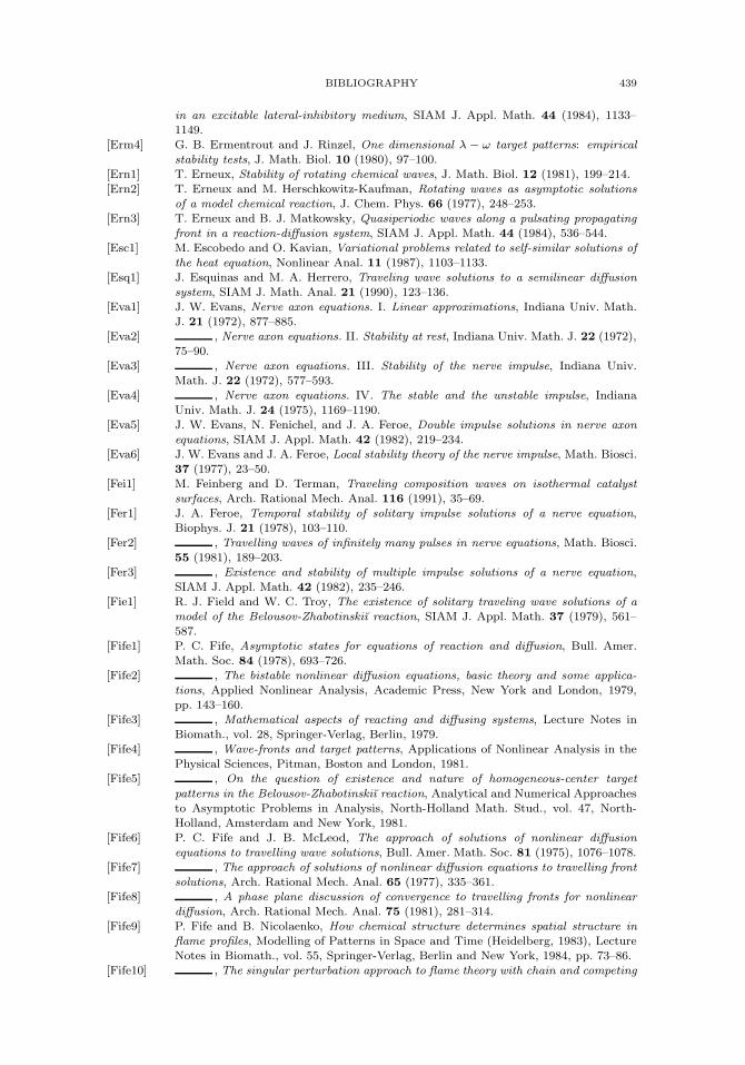
BIBLIOGRAPHY 439
in an excitable lateral-inhibitory medium, SIAM J. Appl. Math. 44 (1984), 1133–1149.
[Erm4] G. B. Ermentrout and J. Rinzel, One dimensional λ − ω target patterns: empiricalstability tests, J. Math. Biol. 10 (1980), 97–100.
[Ern1] T. Erneux, Stability of rotating chemical waves, J. Math. Biol. 12 (1981), 199–214.[Ern2] T. Erneux and M. Herschkowitz-Kaufman, Rotating waves as asymptotic solutions
of a model chemical reaction, J. Chem. Phys. 66 (1977), 248–253.[Ern3] T. Erneux and B. J. Matkowsky, Quasiperiodic waves along a pulsating propagating
front in a reaction-diffusion system, SIAM J. Appl. Math. 44 (1984), 536–544.[Esc1] M. Escobedo and O. Kavian, Variational problems related to self-similar solutions of
the heat equation, Nonlinear Anal. 11 (1987), 1103–1133.[Esq1] J. Esquinas and M. A. Herrero, Traveling wave solutions to a semilinear diffusion
system, SIAM J. Math. Anal. 21 (1990), 123–136.[Eva1] J. W. Evans, Nerve axon equations. I. Linear approximations, Indiana Univ. Math.
J. 21 (1972), 877–885.[Eva2] , Nerve axon equations. II. Stability at rest, Indiana Univ. Math. J. 22 (1972),
75–90.[Eva3] , Nerve axon equations. III. Stability of the nerve impulse, Indiana Univ.
Math. J. 22 (1972), 577–593.[Eva4] , Nerve axon equations. IV. The stable and the unstable impulse, Indiana
Univ. Math. J. 24 (1975), 1169–1190.[Eva5] J. W. Evans, N. Fenichel, and J. A. Feroe, Double impulse solutions in nerve axon
equations, SIAM J. Appl. Math. 42 (1982), 219–234.[Eva6] J. W. Evans and J. A. Feroe, Local stability theory of the nerve impulse, Math. Biosci.
37 (1977), 23–50.[Fei1] M. Feinberg and D. Terman, Traveling composition waves on isothermal catalyst
surfaces, Arch. Rational Mech. Anal. 116 (1991), 35–69.[Fer1] J. A. Feroe, Temporal stability of solitary impulse solutions of a nerve equation,
Biophys. J. 21 (1978), 103–110.[Fer2] , Travelling waves of infinitely many pulses in nerve equations, Math. Biosci.
55 (1981), 189–203.[Fer3] , Existence and stability of multiple impulse solutions of a nerve equation,
SIAM J. Appl. Math. 42 (1982), 235–246.[Fie1] R. J. Field and W. C. Troy, The existence of solitary traveling wave solutions of a
model of the Belousov-Zhabotinskiı reaction, SIAM J. Appl. Math. 37 (1979), 561–587.
[Fife1] P. C. Fife, Asymptotic states for equations of reaction and diffusion, Bull. Amer.Math. Soc. 84 (1978), 693–726.
[Fife2] , The bistable nonlinear diffusion equations, basic theory and some applica-tions, Applied Nonlinear Analysis, Academic Press, New York and London, 1979,pp. 143–160.
[Fife3] , Mathematical aspects of reacting and diffusing systems, Lecture Notes inBiomath., vol. 28, Springer-Verlag, Berlin, 1979.
[Fife4] , Wave-fronts and target patterns, Applications of Nonlinear Analysis in thePhysical Sciences, Pitman, Boston and London, 1981.
[Fife5] , On the question of existence and nature of homogeneous-center target
patterns in the Belousov-Zhabotinskiı reaction, Analytical and Numerical Approachesto Asymptotic Problems in Analysis, North-Holland Math. Stud., vol. 47, North-Holland, Amsterdam and New York, 1981.
[Fife6] P. C. Fife and J. B. McLeod, The approach of solutions of nonlinear diffusionequations to travelling wave solutions, Bull. Amer. Math. Soc. 81 (1975), 1076–1078.
[Fife7] , The approach of solutions of nonlinear diffusion equations to travelling frontsolutions, Arch. Rational Mech. Anal. 65 (1977), 335–361.
[Fife8] , A phase plane discussion of convergence to travelling fronts for nonlineardiffusion, Arch. Rational Mech. Anal. 75 (1981), 281–314.
[Fife9] P. Fife and B. Nicolaenko, How chemical structure determines spatial structure inflame profiles, Modelling of Patterns in Space and Time (Heidelberg, 1983), LectureNotes in Biomath., vol. 55, Springer-Verlag, Berlin and New York, 1984, pp. 73–86.
[Fife10] , The singular perturbation approach to flame theory with chain and competing
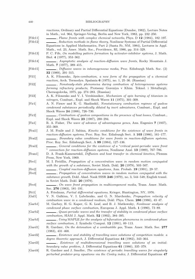
440 BIBLIOGRAPHY
reactions, Ordinary and Partial Differential Equations (Dundee, 1982), Lecture Notesin Math., vol. 964, Springer-Verlag, Berlin and New York, 1982, pp. 232–250.
[Fife11] , Flame fronts with complex chemical networks, Phys. D 12 (1984), 182–197.[Fife12] , Reduction methods in flame theory, Nonlinear Systems of Partial Differential
Equations in Applied Mathematics, Part 2 (Santa Fe, NM, 1984), Lectures in Appl.Math., vol. 23, Amer. Math. Soc., Providence, RI, 1986, pp. 314–329.
[Fife13] P. C. Fife, On modelling pattern formation by activator-inhibitor systems, J. Math.Biol. 4 (1977), 353–362.
[Fife14] , Asymptotic analysis of reaction-diffusion wave fronts, Rocky Mountain J.Math. 7 (1977), 389–415.
[Fife15] , Diffusive waves in inhomogeneous media, Proc. Edinburgh Math. Soc. (2)32 (1989), 291–315.
[Fil1] A. K. Filonenko, Spin-combustion, a new form of the propagation of a chemicalreaction, Arch. Termodyn. Spalania 6 (1975), no. 1, 25–36. (Russian)
[Fil2] , Nonsteady-state phenomena during combustion of heterogeneous systemsforming refractory products, Protsessy Goreniya v Khim. Teknol. i Metallurgii,Chernogolovka, 1975, pp. 274–283. (Russian)
[Fil3] A. K. Filonenko and V. I. Vershinnikov, Mechanism of spin burning of titanium innitrogen, Combust., Expl. and Shock Waves 11 (1975), 301–309.
[Fir1] A. N. Firsov and K. G. Skadinskiı, Nonstationary combustion regimes of gaslesscondensed substances periodically diluted by inert admixtures, Combust., Expl. andShock Waves 24 (1988), 726–730.
[Fir2] , Combustion of gasless compositions in the presence of heat losses, Combust.,Expl. and Shock Waves 23 (1987), 288–294.
[Fis1] R. A. Fisher, The wave of advance of advantageous genes, Ann. Eugenics 7 (1937),355–369.
[Frai1] J. M. Fraile and J. Sabina, Kinetic conditions for the existence of wave fronts inreaction-diffusion systems, Proc. Roy. Soc. Edinburgh Sect. A 103 (1986), 161–177.
[Frai2] , Boundary value conditions for wave fronts in reaction-diffusion systems,Proc. Roy. Soc. Edinburgh Sect. A 99 (1984), 127–136.
[Frai3] , General conditions for the existence of a “critical point-periodic wave front” connection for reaction-diffusion systems, Nonlinear Anal. 13 (1989), 767–786.
[Fran1] D. A. Frank-Kamenetskiı, Diffusion and heat transfer in chemical kinetics, PlenumPress, New York, 1969.
[Fre1] M. I. Freidlin, Propagation of a concentration wave in random motion conjugatedwith the growth of a substance, Soviet Math. Dokl. 20 (1979), 503–507.
[Fre2] , Coupled reaction-diffusion equations, Ann. Probab. 19 (1991), 29–57.[Fre3] , Propagation of concentration waves in random motion conjugated with the
substance growth, Dokl. Akad. Nauk SSSR 246 (1979), no. 3, 544–548; English transl.in Soviet Math. Dokl. 20 (1979).
[Fre4] , On wave front propagation in multicomponent media, Trans. Amer. Math.Soc. 276 (1983), 181–191.
[Fri1] A. Friedman, Partial differential equations, Krieger, Huntington, NY, 1976.[Gal1] V. N. Galkina, V. I. Lubchenko, and G. N. Marchenko, Propagation velocity of
combustion wave in a condensed medium, Dokl. Phys. Chem. 286 (1986), 43–47.[Garb1] M. Garbey, H. G. Kaper, G. K. Leaf, and B. J. Matkowsky, Nonlinear analysis of
condensed phase surface combustion, European J. Appl. Math. 1 (1990), 73–89.[Garb2] , Quasi-periodic waves and the transfer of stability in condensed phase surface
combustion, SIAM J. Appl. Math. 52 (1992), 384–395.[Garb3] , Using MAPLE for the analysis of bifurcation phenomena in condensed-phase
surface combustion, J. Symbolic Comput. 12 (1991), 89–113.[Gard1] R. Gardner, On the detonation of a combustible gas, Trans. Amer. Math. Soc. 277
(1983), 431–468.[Gard2] , Existence and stability of travelling wave solutions of competition models: a
degree theoretic approach, J. Differential Equations 44 (1982), 343–364.[Gard3] , Existence of multidimensional travelling wave solutions of an initial-
boundary value problem, J. Differential Equations 61 (1986), 335–379.[Gard4] R. Gardner and J. Smoller, The existence of periodic travelling waves for singularly
perturbed predator-prey equations via the Conley index, J. Differential Equations 47
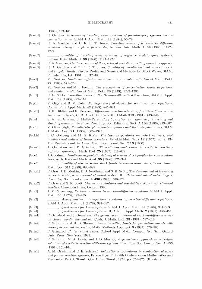
BIBLIOGRAPHY 441
(1983), 133–161.[Gard5] R. Gardner, Existence of traveling wave solutions of predator–prey systems via the
connection index, SIAM J. Appl. Math. 44 (1984), 56–79.[Gard6] R. A. Gardner and C. K. R. T. Jones, Traveling waves of a perturbed diffusion
equation arising in a phase field model, Indiana Univ. Math. J. 39 (1990), 1197–1222.
[Gard7] , Stability of traveling wave solutions of diffusive predator-prey systems,Indiana Univ. Math. J. 39 (1990), 1197–1222.
[Gard8] R. A. Gardner, On the structure of the spectra of periodic travelling waves (to appear).[Gard9] R. A. Gardner and C. K. R. T. Jones, Stability of one-dimensional waves in weak
and singular limits, Viscous Profile and Numerical Methods for Shock Waves, SIAM,Philadelphia, PA, 1991, pp. 32–48.
[Ger1] Yu. Gertner, Nonlinear diffusion equations and excitable media, Soviet Math. Dokl.22 (1980), 571–574.
[Ger2] Yu. Gertner and M. I. Freidlin, The propagation of concentration waves in periodicand random media, Soviet Math. Dokl. 20 (1979), 1282–1286.
[Gib1] R. G. Gibbs, Travelling waves in the Belousov-Zhabotinskiı reaction, SIAM J. Appl.Math. 38 (1980), 422–444.
[Gig1] Y. Giga and R. V. Kohn, Nondegeneracy of blowup for semilinear heat equations,Comm. Pure Appl. Math. 42 (1989), 845–884.
[Gild1] B. H. Gilding and R. Kersner, Diffusion-convection-reaction, frontieres libres et uneequation integrale, C. R. Acad. Sci. Paris Ser. I Math 313 (1991), 743–746.
[Gils1] S. A. van Gils and J. Mallet-Paret, Hopf bifurcation and symmetry: travelling andstanding waves on the circle, Proc. Roy. Soc. Edinburgh Sect. A 104 (1986), 279–307.
[Gio1] V. Giovangigli, Nonadiabatic plane laminar flames and their singular limits, SIAMJ. Math. Anal. 21 (1990), 1305–1325.
[Gokh1] I. C. Gohberg and M. G. Kreın, The basis propositions on defect numbers, rootnumbers and indices of linear operators, Uspekhi Mat. Nauk 12 (1957), no. 2, 43–118; English transl. in Amer. Math. Soc. Transl. Ser. 2 13 (1960).
[Gom1] J. Gomatam and P. Grindrod, Three-dimensional waves in excitable reaction-diffusion systems, J. Math. Biol. 25 (1987), 611–622.
[Goo1] J. Goodman, Nonlinear asymptotic stability of viscous shock profiles for conservationlaws, Arch. Rational Mech. Anal. 95 (1986), 325–344.
[Goo2] , Stability of viscous scalar shock fronts in several dimensions, Trans. Amer.Math. Soc. 311 (1989), 683–695.
[Gray1] P. Gray, J. H. Merkin, D. J. Needham, and S. K. Scott, The development of travellingwaves in a simple isothermal chemical system. III. Cubic and mixed autocatalysis,Proc. Roy. Soc. London Ser. A 430 (1990), 509–524.
[Gray2] P. Gray and S. K. Scott, Chemical oscillations and instabilities. Non-linear chemicalkinetics, Clarendon Press, Oxford, 1990.
[Gre1] J. M. Greenberg, Periodic solutions to reaction-diffusion equations, SIAM J. Appl.Math. 30 (1976), 199–205.
[Gre2] , Axi-symmetric, time-periodic solutions of reaction-diffusion equations,SIAM J. Appl. Math. 34 (1978), 391–397.
[Gre3] , Spiral waves for λ − ω systems, SIAM J. Appl. Math. 39 (1980), 301–309.[Gre4] , Spiral waves for λ − ω systems. II, Adv. in Appl. Math. 2 (1981), 450–454.[Grin1] P. Grindrod and J. Gomatam, The geometry and motion of reaction-diffusion waves
on closed two-dimensional manifolds, J. Math. Biol. 25 (1987), 597–610.[Grin2] P. Grindrod and B. D. Sleeman, Weak travelling fronts for population models with
density dependent dispersion, Math. Methods Appl. Sci. 9 (1987), 576–586.[Grin3] P. Grindrod, Patterns and waves, Oxford Appl. Math. Comput. Sci. Ser., Oxford
Univ. Press, New York, 1991.[Grin4] P. Grindrod, M. A. Lewis, and J. D. Murray, A geometrical approach to wave-type
solutions of excitable reaction-diffusion systems, Proc. Roy. Soc. London Ser. A 433(1991), 151–164.
[Gris1] A. M. Grishin and E. E. Zelenskiı, Relaxational oscillations in combustion of gasesand porous reacting systems, Proceedings of the 4th Conference on Mathematics andMechanics, Part 2, Tomsk. Gos. Univ., Tomsk, 1974, pp. 674–675. (Russian)
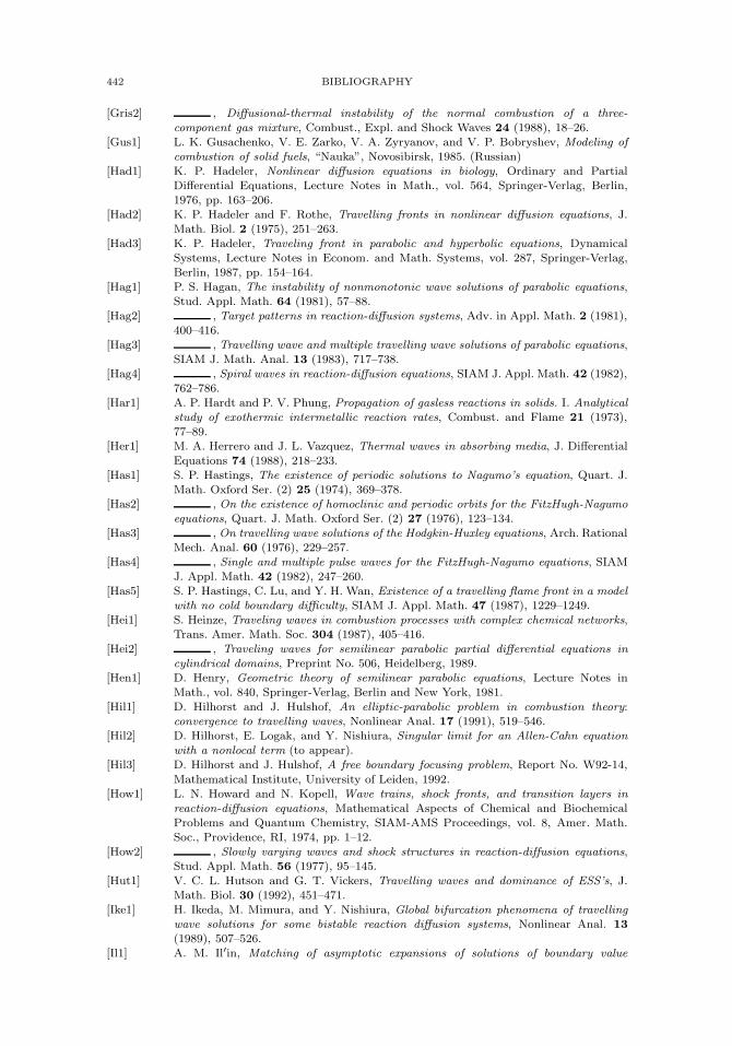
442 BIBLIOGRAPHY
[Gris2] , Diffusional-thermal instability of the normal combustion of a three-component gas mixture, Combust., Expl. and Shock Waves 24 (1988), 18–26.
[Gus1] L. K. Gusachenko, V. E. Zarko, V. A. Zyryanov, and V. P. Bobryshev, Modeling ofcombustion of solid fuels, “Nauka”, Novosibirsk, 1985. (Russian)
[Had1] K. P. Hadeler, Nonlinear diffusion equations in biology, Ordinary and PartialDifferential Equations, Lecture Notes in Math., vol. 564, Springer-Verlag, Berlin,1976, pp. 163–206.
[Had2] K. P. Hadeler and F. Rothe, Travelling fronts in nonlinear diffusion equations, J.Math. Biol. 2 (1975), 251–263.
[Had3] K. P. Hadeler, Traveling front in parabolic and hyperbolic equations, DynamicalSystems, Lecture Notes in Econom. and Math. Systems, vol. 287, Springer-Verlag,Berlin, 1987, pp. 154–164.
[Hag1] P. S. Hagan, The instability of nonmonotonic wave solutions of parabolic equations,Stud. Appl. Math. 64 (1981), 57–88.
[Hag2] , Target patterns in reaction-diffusion systems, Adv. in Appl. Math. 2 (1981),400–416.
[Hag3] , Travelling wave and multiple travelling wave solutions of parabolic equations,SIAM J. Math. Anal. 13 (1983), 717–738.
[Hag4] , Spiral waves in reaction-diffusion equations, SIAM J. Appl. Math. 42 (1982),762–786.
[Har1] A. P. Hardt and P. V. Phung, Propagation of gasless reactions in solids. I. Analyticalstudy of exothermic intermetallic reaction rates, Combust. and Flame 21 (1973),77–89.
[Her1] M. A. Herrero and J. L. Vazquez, Thermal waves in absorbing media, J. DifferentialEquations 74 (1988), 218–233.
[Has1] S. P. Hastings, The existence of periodic solutions to Nagumo’s equation, Quart. J.Math. Oxford Ser. (2) 25 (1974), 369–378.
[Has2] , On the existence of homoclinic and periodic orbits for the FitzHugh-Nagumoequations, Quart. J. Math. Oxford Ser. (2) 27 (1976), 123–134.
[Has3] , On travelling wave solutions of the Hodgkin-Huxley equations, Arch. RationalMech. Anal. 60 (1976), 229–257.
[Has4] , Single and multiple pulse waves for the FitzHugh-Nagumo equations, SIAMJ. Appl. Math. 42 (1982), 247–260.
[Has5] S. P. Hastings, C. Lu, and Y. H. Wan, Existence of a travelling flame front in a modelwith no cold boundary difficulty, SIAM J. Appl. Math. 47 (1987), 1229–1249.
[Hei1] S. Heinze, Traveling waves in combustion processes with complex chemical networks,Trans. Amer. Math. Soc. 304 (1987), 405–416.
[Hei2] , Traveling waves for semilinear parabolic partial differential equations incylindrical domains, Preprint No. 506, Heidelberg, 1989.
[Hen1] D. Henry, Geometric theory of semilinear parabolic equations, Lecture Notes inMath., vol. 840, Springer-Verlag, Berlin and New York, 1981.
[Hil1] D. Hilhorst and J. Hulshof, An elliptic-parabolic problem in combustion theory:convergence to travelling waves, Nonlinear Anal. 17 (1991), 519–546.
[Hil2] D. Hilhorst, E. Logak, and Y. Nishiura, Singular limit for an Allen-Cahn equationwith a nonlocal term (to appear).
[Hil3] D. Hilhorst and J. Hulshof, A free boundary focusing problem, Report No. W92-14,
Mathematical Institute, University of Leiden, 1992.[How1] L. N. Howard and N. Kopell, Wave trains, shock fronts, and transition layers in
reaction-diffusion equations, Mathematical Aspects of Chemical and BiochemicalProblems and Quantum Chemistry, SIAM-AMS Proceedings, vol. 8, Amer. Math.Soc., Providence, RI, 1974, pp. 1–12.
[How2] , Slowly varying waves and shock structures in reaction-diffusion equations,Stud. Appl. Math. 56 (1977), 95–145.
[Hut1] V. C. L. Hutson and G. T. Vickers, Travelling waves and dominance of ESS’s, J.Math. Biol. 30 (1992), 451–471.
[Ike1] H. Ikeda, M. Mimura, and Y. Nishiura, Global bifurcation phenomena of travellingwave solutions for some bistable reaction diffusion systems, Nonlinear Anal. 13(1989), 507–526.
[Il1] A. M. Il′in, Matching of asymptotic expansions of solutions of boundary value
BIBLIOGRAPHY 443
problems, “Nauka”, Moscow, 1989; English transl., Transl. Math. Monographs,vol. 102, Amer. Math. Soc., Providence, RI, 1992.
[Il2] A. M. Il′in and O. A. Oleınik, Behavior of solutions of the Cauchy problem for certainquasilinear equations for unbounded increase of the time, Dokl. Akad. Nauk SSSR120 (1958), 25–28; English transl. in Amer. Math. Soc. Transl. Ser. 2 42 (1964).
[Il3] , Asymptotic behavior of solutions of the Cauchy problem for some quasi-linear equations for large values of the time, Mat. Sb. 51 (1960), no. 2, 191–216.(Russian)
[Il4] A. M. Il′in and S. I. Khudyaev, On the asymptotics of stationary combustion wavein condensed medium, Khimicheskaya Fizika 8 (1989), no. 4, 525–532; English transl.in Soviet J. Chem. Phys.
[Iva1] G. R. Ivanitsky, V. I. Krinskiı, and E. E. Sel′kov, Mathematical biophysics of cells,“Nauka”, Moscow, 1978. (Russian)
[Ivl1] T. P. Ivleva, A. G. Merzhanov, and K. G. Skadinskiı, Principles of the spin mode ofcombustion front propagation, Combust., Expl. and Shock Waves 16 (1980), 133–139.
[Ivl2] , Mathematical model of spin combustion, Soviet Phys. Dokl. 23 (1978), 255–256.
[Ivl3] T. P. Ivleva and K. G. Skadinskiı, On a regime of burning of a thin plate, FizikaGoreniya i Vzryva 17 (1981), no. 1, 138–140. (Russian)
[Ito1] M. Ito, Travelling train solutions of FitzHugh-Nagumo systems, Recent Topics inNonlinear PDE III (Tokyo, 1986), North-Holland Math. Stud., vol. 148, NorthHolland, Amsterdam and New York, 1987, pp. 75–104.
[Jon1] C. K. R. T. Jones, Spherically symmetric solutions of a reaction-diffusion equation,J. Differential Equations 49 (1983), 142–169.
[Jon2] , Asymptotic behaviour of a reaction-diffusion equation in higher spacedimensions, Rocky Mountain J. Math. 13 (1983), 355–364.
[Jon3] , Stability of the travelling wave solutions of the FitzHugh-Nagumo system,Trans. Amer. Math. Soc. 286 (1984), 431–469.
[Jon4] C. Jones, R. Gardner, and T. Kapitula, Stability of travelling waves for non-convexscalar viscous conservation laws, Comm. Pure Appl. Math. 46 (1993), 505–526.
[Jou1] G. Joulin and P. Clavin, Asymptotic analysis of a premixed laminar flame governedby a two-step reaction, Combust. and Flame 23 (1975), 389–392.
[Jou2] , Asymptotic analysis of conditions of extinction for laminar flames, ActaAstronautica 3 (1976), 223–240.
[Jou3] , Linear stability analysis of nonadiabatic flames: diffusional thermal model,Combust. and Flame 35 (1979), 139–153.
[Kag1] Z. I. Kaganova, Secondary limit of isothermal flame propagation during decompo-sition of nitrogen chloride (NCl3), Khimicheskaya Fizika 3 (1984), no. 3, 292–294;English transl. in Soviet J. Chem. Phys.
[Kag2] , Heterogeneous mechanism of isothermal flame propagation, KhimicheskayaFizika 3 (1984), no. 4, 598–602; English transl. in Soviet J. Chem. Phys.
[Kag3] Z. I. Kaganova and B. V. Novozhilov, Kinetics of branched chain reactions in thepresence of an inhibitor, Kinetics and Catalysis 21 (1980), 972–977.
[Kag4] , Inverse problem of the theory of combustion as exemplified by an isothermal
flame of nitrogen trichloride decomposition, Khimicheskaya Fizika 1 (1982), no. 8,1110–1121; English transl. in Soviet J. Chem. Phys.
[Kalan1] V. K. Kalantarov and O. A. Ladyzhenskaya, Stabilization of solutions of a certainclass of quasilinear parabolic equations as t → ∞, Siberian Math. J. 19 (1978),737–744.
[Kalen1] A. Kalen, Thresholds and travelling waves in an epidemic model for rabies, NonlinearAnal. 8 (1984), 851–856.
[Kam1] Y. Kametaka, On the nonlinear diffusion equation of Kolmogorov-Petrovskiı-Piskunov type, Osaka J. Math. 13 (1976), 11–66.
[Kan1] Ya. I. Kanel′, The behavior of solutions of the Cauchy problem when the time tendsto infinity, in the case of quasilinear equations arising in the theory of combustion,Soviet Math. Dokl. 1 (1960), 533–536.
[Kan2] , Some problems involving burning-theory equations, Soviet Math. Dokl. 2(1961), 48–51.
444 BIBLIOGRAPHY
[Kan3] , Stabilization of solutions of the Cauchy problem for equations encounteredin combustion theory, Mat. Sb. 101 (1962), 245–288. (Russian)
[Kan4] , The stationary solution of the set of equations in the theory of combustion,Dokl. Phys. Chem. 149 (1963), 241–243.
[Kan5] , Stabilization of the solutions of the equations of combustion theory with finiteinitial functions, Mat. Sb. 107 (1964), 398–413. (Russian)
[Kan6] , The existence of a solution of traveling wave type for the Belousov-Zhabotinskiı system of equations, J. Differential Equations 26 (1990), 478–485.
[Kan7] , The existence of the solutions of traveling wave type for the Belousov-Zhabotinskiı system of equations. II, Siberian Math. J. 32 (1992), 390–400.
[Kant1] L. V. Kantorovich and G. P. Akilov, Functional analysis, “Nauka”, Moscow, 1977;English transl., Pergamon Press, Oxford, 1982.
[Kape1] H. G. Kaper, G. K. Leaf, S. B. Margolis, and B. J. Matkowsky, On nonadiabaticcondensed phase combustion, Combust. Sci. and Technol. 53 (1987), 289–314.
[Kapi1] A. K. Kapila and G. S. Ludford, Two-step sequential reactions for large activationenergies, Combust. and Flame 29 (1977), 167–176.
[Kee1] J. P. Keener, Waves in excitable media, SIAM J. Appl. Math. 39 (1980), 528–548.[Kee2] , A geometrical theory for spiral waves in excitable media, SIAM J. Appl.
Math. 46 (1986), 1039–1056.[Kern1] M. Kern, On the stability and instability of autowaves of reaction-diffusion systems,
Math. Nachr. 141 (1989), 81–100.[Kha1] B. I. Khaikin, Heterogeneous combustion, Heat and Mass Transfer in Combustion
Processes, Inst. Chem. Phys., Chernogolovka, 1980, pp. 58–79. (Russian)[Kha2] B. I. Khaikin and A. G. Merzhanov, Theory of thermal propagation of a chemical
reaction front, Combust., Expl. and Shock Waves 2 (1966), 22–27.[Kha3] B. I. Khaikin, A. K. Filonenko, and S. I. Khudyaev, Flame propagation in the presence
of two successive gas-phase reactions, Combust., Expl. and Shock Waves 4 (1968),343–349.
[Kha4] B. I. Khaikin and S. I. Khudyaev, On nonuniqueness of stationary propagatingreaction zones with competing reactions, Preprint, Inst. Chem. Phys., Chernogolovka,1978. (Russian)
[Kha5] , Nonuniqueness of combustion temperature and rate when competing reac-tions take place, Dokl. Phys. Chem. 245 (1979), 225–228.
[Kha6] B. I. Khaikin, S. I. Khudyaev, and L. A. Zhukova, Nonuniqueness, stability andpulsating regimes of combustion with competing reactions, Chemical Physics of theProcesses of Combustion and Explosion. Combustion of Condensed and Heteroge-neous Systems, Inst. Chem. Phys., Chernogolovka, 1980, pp. 28–32. (Russian)
[Kha7] B. I. Khaikin and S. I. Khudyaev, On nonuniqueness of stationary combustion waves,Preprint, Inst. Chem. Phys., Chernogolovka, 1981. (Russian)
[Kha8] B. I. Khaikin and K. G. Skadinskiı, Effect of heat losses on propagation of the frontof exothermal reaction in condensed phase, Combustion and Explosion (Proc. III All-Union Symposium on Combustion and Explosion), “Nauka”, Moscow, 1972, pp. 24-29. (Russian)
[Kha9] B. I. Khaikin and E. N. Rumanov, Exothermic reaction regimes in a one-dimensional
flow, Combust., Expl. and Shock Waves 11 (1975), 573–579.[Khu1] S. I. Khudyaev, Mathematical theory of combustion and explosion, Preprint, Inst.
Chem. Phys., Chernogolovka, 1980. (Russian)[Khu2] , Asymptotic theory of stationary combustion waves, Khimicheskaya Fizika 6
(1987), no. 5, 681–691; English transl. in Soviet J. Chem. Phys.[Kir1] K. Kirchgassner, Wave solutions of reversible systems and applications, J. Differential
Equations 45 (1982), 113–127.[Kir2] , Waves in weakly-coupled parabolic systems, Nonlinear Analysis and Opti-
mization, Lecture Notes in Math., vol. 1107, Springer-Verlag, Berlin and New York,1984, pp. 154–180.
[Kis1] O. V. Kiselev, and Yu. Sh. Matros, and N. A. Chumakova, On propagation ofthe thermal front through the catalyst layer, Propagation of Thermal Waves inHeterogeneous Media, “Nauka”, Novosibirsk, 1988, pp. 145–203. (Russian)
[Kla1] G. A. Klaasen and W. C. Troy, The stability of traveling wave front solution of areaction-diffusion system, SIAM J. Appl. Math. 41 (1981), 145–167.
BIBLIOGRAPHY 445
[Kla2] , The asymptotic behavior of solutions of a system of reaction-diffusionequations which models the Belousov-Zhabotinskiı chemical reaction, J. DifferentialEquations 40 (1981), 253–278.
[Kla3] , Stationary wave solutions of a system of reaction-diffusion equations derivedfrom FitzHugh-Nagumo equations, SIAM J. Appl. Math. 44 (1984), 96–110.
[Koga1] S. Koga, Rotating spiral waves in reaction-diffusion systems. Phase singularities ofmulti-armed waves, Progr. Theoret. Phys. 67 (1982), 164–178.
[Kole1] A. Yu. Kolesov, A criterion for the stability of traveling waves of parabolic systemswith small diffusion, Siberian Math. J. 30 (1989), 484–488.
[Kole2] Yu. S. Kolesov, Stability and bifurcations of traveling waves, Nonlinear Fluctuationsin Problems of Ecology, Yaroslav. Gos. Univ., Yaroslavl′, 1985, pp. 3–10. (Russian)
[Kolm1] A. N. Kolmogorov, I. G. Petrovskiı, and N. S. Piskunov, Etude de l’equation de lachaleur avec croissance de la quantite de matiere et son application a un problemebiologique, Bull. Moskov. Gos. Univ. Mat. Mekh. 1 (1937), no. 6, 1–25. (Russian)
[Kon1] V. N. Kondrat′ev, The mechanism of carbon disulfide oxidation, Kinetics andCatalysis 13 (1972), 1223–1235.
[Kop1] N. J. Kopell, Waves, shocks and target patterns in an oscillating chemical reagent,Nonlinear Diffussion, Res. Notes Math., No. 14, Pitman, London, 1977, pp. 129–154.
[Kop2] , Target pattern solutions to reaction-diffusion equations in the presence ofimpurities, Adv. in Appl. Math. 2 (1981), 389–399.
[Kop3] N. Kopell and L. N. Howard, Plane wave solutions to reaction-diffusion equations,Stud. Appl. Math. 52 (1973), 291–328.
[Kop4] , Bifurcations and trajectories joining critical points, Adv. Math. 18 (1975),306–358.
[Kop5] , Target patterns and horseshoes from perturbed central-force problems : sometemporally periodic solutions to reaction-diffusion equations, Stud. Appl. Math. 64(1981), 1–56.
[Kop6] , Target patterns and spiral solutions to reaction-diffusion equations with morethan one space dimension, Adv. Appl. Math. 2 (1989), 417–449.
[Kor1] H. F. Korman, Theoretical modeling of cold flames, Combust. Sci. and Technol. 2(1970), 149–159.
[Koro1] A. P. Korostelev and M. I. Freidlin, On propagation of concentrational waves dueto nonlinear boundary effects, Factors of Variety in Mathematical Ecology andPopulational Genetics, Pushchino, 1980. (Russian)
[Korob1] O. P. Korobeinichev (ed.), Flame structure, vol. 1–2, “Nauka”, Novosibirsk, 1991.(Russian)
[Kra1] M. A. Krasnoselskiı, Positive solutions of operator equations, Noordhoff, Groningen,1964.
[Kra2] M. A. Krasnoselskiı and P. P. Zabreiko, Geomertical methods of nonlinear analysis,Grundlehren Math. Wiss, vol. 263, Springer-Verlag, Berlin and New York, 1984.
[Kra3] M. A. Krasnoselskiı, P. P. Zabreiko, E. I. Pustyl′nik, and P. E. Sobolevskiı, Integraloperators in spaces of summable functions, Noordhoff, Leiden, 1976.
[Kri1] V. I. Krinskiı, Fibrillation in excitable media, Problemi Kibernetiki 20 (1968), 59–80.(Russian)
[Kri2] V. I. Krinskiı and K. I. Agladze, Vortices with topological charge 2, 3, and 4 in anactive chemical medium, Soviet Phys. Dokl. 27 (1982), 228–229.
[Kri3] V. I. Krinskiı, Mathematical models of cardiac arhythmias (spiral waves), Pharmac.Ther. B. 3 (1978), 539–555.
[Kuz1] Yu. A. Kuznetsov, Existence and stability of traveling waves for reaction diffusionsystems in one dimension, Preprint, NIVT, 1982. (Russian)
[Lad1] O. A. Ladyzhenskaya and N. N. Ural′tseva, Linear and quasilinear elliptic equations,Academic Press, New York and London, 1968.
[Lan1] P. S. Landa, Self-oscillations in distributed systems, “Nauka”, Moscow, 1983.(Russian)
[Lar1] D. Larson, On the stability of certain wave solutions to Nagumo’s equation, Quart.J. Math. Oxford Ser. (2) 28 (1977), 339–352.
[Lar2] , Transient bounds and time-asymptotic behaviour of solutions to nonlinearequations of Fisher type, SIAM J. Appl. Math. 34 (1978), 93–103.
446 BIBLIOGRAPHY
[Ler1] J. Leray and J. Schauder, Topologie et equations fonctionnelle, Ann. Sci. Ecole Norm.Sup. 113 (1934), 45–78.
[Lev1] C. D. Levermore and J. X. Xin, Multidimensional stability of traveling waves ina bistable reaction-diffusion equation. II, Comm. Partial Differential Equations 17(1992), 1901–1924.
[Lew1] B. Lewis and G. von Elbe, Combustion, flames and explosions of gases, AcademicPress, New York, San Francisco, and London, 1961.
[Li1] Z. Y. Li, The existence of traveling front solutions for reaction-diffusion system, J.Partial Differential Equations 5 (1992), 17–22.
[Li2] Z. Y. Li and Q. X. Ye, Traveling wave front solutions for reaction-diffusion systems,J. Partial Differential Equations 4 (1991), 1–14.
[Liu1] Bao-Ping Liu and C. V. Pao, Almost periodic plane wave solutions for reaction-diffusion equations, J. Math. Anal. Appl. 105 (1985), 231–249.
[Liu2] Bao-Ping Liu and Bi Zhao, Multiple periodic plane wave solutions for the FitzHugh-Nagumo nerve conduction equations, Acta Math. Appl. Sinica 12 (1989), 13–23.
[Lua1] Ka-Sing Lua, On the nonlinear diffusion equation of Kolmogorov, Petrovskiı andPiskunov, J. Differential Equations 59 (1985), 44–70.
[Luk1] A. T. Luk′yanov, L. Yu. Artyukh, and P. G. Itskova, Mathematical modeling ofproblems of combustion theory, “Nauka”, Alma-Ata, 1981. (Russian)
[Luk2] , Resonance equilibrium in problems in combustion theory, “Nauka”, Alma-Ata, 1989. (Russian)
[Mag1] K. Maginu, Stability of periodic travelling wave solutions of a nerve conductionequation, J. Math. Biol. 6 (1978), 49–57.
[Mag2] , Existence and stability of periodic travelling wave solutions to Nagumo’snerve equation, J. Math. Biol. 10 (1980), 133–153.
[Mag3] , Stability of periodic travelling wave solutions with large spatial periods inreaction-diffusion systems, J. Differential Equations 39 (1981), 73–99.
[Mag4] , Geometrical characteristics associated with stability and bifurcations ofperiodic travelling waves in reaction-diffusion systems, SIAM J. Appl. Math. 45(1985), 750–774.
[Makh1] G. M. Makhviladze and B. V. Novozhilov, Two-dimensional stability of combustionof condensed systems, Zh. Prikl. Mekh. i Tekhn. Fiz. (1971), no. 5, 51–59; Englishtransl. in J. Appl. Mech. Tech. Phys.
[Makh2] , Two-dimensional combustion stability of condensed systems, Heat Transfer– Soviet Research 5, 37–44.
[Mak1] E. I. Maksimov, A. G. Merzhanov, and V. M. Shkiro, Gasless compositions as asimple model for the combustion of nonvolatile condensed systems, Combust., Expl.and Shock Waves 1 (1965), 15–19.
[Mak2] E. I. Maksimov and K. G. Skadinskiı, Steady-state combustion stability gaslesscompositions, Combust., Expl. and Shock Waves 7 (1971), 392–396.
[Mak3] Yu. M. Maksimov, A. T. Pak, G. V. Lavrenchuk, Yu. S. Naiborodenko, and A. G.Merzhanov, Spin combustion of gasless systems, Combust., Expl. and Shock Waves15 (1979), 415–418.
[Mak4] Yu. M. Maksimov, A. G. Merzhanov, A. T. Pak, and M. N. Kuchkin, Unstable
combustion modes of gasless systems, Combust., Expl. and Shock Waves 17 (1981),393–400.
[Mal1] B. A. Malomed, Some modes for the propagation of auto-oscillatory waves, SovietPhys. Dokl. 26 (1981), 203–205.
[Mar1] S. B. Margolis, An asymptotic theory of condensed two-phase flame propagation,SIAM J. Appl. Math. 43 (1983), 351–369.
[Mar2] , An asymptotic theory of heterogeneous condensed combustion, Combust. Sci.and Technol. 43 (1985), 197–215.
[Mar3] S. B. Margolis and R. M. Green, Theoretical prediction of self-propagating, diffusion-and decomposition limited intermetallic reactions, Combust. and Flame 34 (1979),245–252.
[Mar4] S. B. Margolis, H. G. Kaper, G. K. Leaf, and B. J. Matkowsky, Bifurcation ofpulsating and spinning reaction fronts in condensed two-phase combustion, Combust.Sci. and Technol. 43 (1985), 127–165.
BIBLIOGRAPHY 447
[Mar5] S. B. Margolis and B. J. Matkowsky, Flame propagation with a sequential reactionmechanism, SIAM J. Appl. Math. 42 (1982), 1175–1188.
[Mar6] , Steady and pulsating model of sequential flame propagation, Combust. Sci.and Technol. 27 (1982), 193–213.
[Mar7] , Nonlinear stability and bifurcation in the transition from laminar toturbulent flame propagation, Combust. Sci. and Technol. 34 (1983), 45–77.
[Mar8] , Flame propagation in channels: secondary bifurcation to quasiperiodicpulsations, SIAM J. Appl. Math. 45 (1985), 93–129.
[Mar9] , Flame propagation with multiple fuels, SIAM J. Appl. Math. 42 (1982),982–1003.
[Mar10] , New modes of quasiperiodic combustion near a degenerate Hopf bifurcationpoint, SIAM J. Appl. Math. 48 (1988), 828–853.
[Mars1] J. Marsden and M. McCracken, The Hopf bifurcation and its applications, Appl.Math. Sci., vol. 19, Springer-Verlag, New York, 1976.
[Mas1] V. P. Maslov, V. G. Danilov, and K. A. Volosov, Mathematical modeling of heat andmass-transport processes, “Nauka”, Moscow, 1987. (Russian)
[Mat1] B. J. Matkowsky and G. I. Sivashinsky, Propagation of a pulsating reaction front insolid fuel combustion, SIAM J. Appl. Math. 35 (1978), 465–478.
[Mat2] , An asymptotic derivation of two models in flame theory associated with theconstant density approximation, SIAM J. Appl. Math. 37 (1979), 686–699.
[Mat3] B. J. Matkowsky and D. O. Olagunju, Propagation of a pulsating flame front in agaseous combustible mixture, SIAM J. Appl. Math. 39 (1980), 290–300.
[Mat4] , Pulsations in a burner stabilized premixed plane flame, SIAM J. Appl. Math.40 (1981), 551–562.
[Mat5] , Traveling waves along the front of a pulsating flame, SIAM J. Appl. Math.42 (1982), 486–501.
[Mat6] , Spinning waves in gaseous combustion, SIAM J. Appl. Math. 42 (1982),1138–1156.
[Mat7] B. J. Matkowsky and G. I. Sivashinsky, On oscillatory necking in polymers, Quart.Appl. Math. 37 (1979), 23–34.
[McK1] H. P. McKean, Application of Brownian motion to the equation of Kolmogorov-Petrovskiı-Piskunov, Comm. Pure Appl. Math. 28 (1975), 323–331; A correctionto: “Application of Brownian motion to the equation of Kolmogorov-Petrovskiı-Piskunov”, Comm. Pure Appl. Math. 29 (1976), 553–554.
[McK2] , Stabilization of solutions of a caricature of the FitzHugh-Nagumo equation.II, Comm. Pure Appl. Math. 37 (1984), 299–301.
[Meg1] I. N. Megrabova, Vit. A. Volpert, Vl. A. Volpert, and S. P. Davtyan, Two-dimensionalchemical reaction regimes in a flow, Dokl. Phys. Chem. 307 (1989), 618–620.
[Meg2] , Two-dimensional combustion conditions in flow, Combust., Expl. and ShockWaves 26 (1990), 413–417.
[Mer1] A. G. Merzhanov, Theory of gasless combustion, Archiwum Procesow Spalania 5(1974), no. 1, 17–39. (Russian)
[Mer2] , Self-propagating high-temperature synthesis, Physical Chemistry. Present-Day Problems, Khimiya, Moscow, 1983, pp. 5–45. (Russian)
[Mer3] , New elementary combustion models of the second kind, Dokl. Phys. Chem.233 (1977), 430–434.
[Mer4] A. G. Merzhanov, I. P. Borovinskaya, and V. M. Shkiro, Synthesis of refractoryinorganic compounds, Patent Certif. 255221, Appl. No. 1170735, 1967.
[Mer5] A. G. Merzhanov, A. V. Dvoryankin, and A. G. Strunina, New type of spin burning,Dokl. Phys. Chem. 267 (1983), 979–981.
[Mer6] A. G. Merzhanov, E. N. Rumanov, and B. I. Khaikin, Multizone burning of condensedsystems, Zh. Prikl. Mekh. i Tekhn. Fiz. (1972), no. 6, 99–105; English transl. in J.Appl. Mech. Tech. Phys.
[Mer7] A. G. Merzhanov, A. K. Filonenko, and I. P. Borovinskaya, New phenomena incombustion of condensed systems, Dokl. Phys. Chem. 208 (1973), 122–125.
[Mer8] A. G. Merzhanov and B. I. Khaikin, Theory of combustion waves in homogeneousmedia, Progr. Energy Combust. Sci. 14 (1988), 1–98.
[Mer9] A. G. Merzhanov and A. K. Filonenko, Thermal self-ignition of a homogeneous gasmixture in a stream, Dokl. Phys. Chem. 152 (1963), 769–772.
448 BIBLIOGRAPHY
[Mim1] M. Mimura, Wave propagation and its failure in bistable reaction-diffusion systems,Nonlinear Analysis, World Sci. Publishing, Teaneck, NJ, 1991, pp. 185–222.
[Mis1] K. Mischaikow, Traveling waves for a cooperative and competitive-cooperative system,Viscous Profiles and Numerical Methods for Shock Waves, SIAM, Philadelphia, PA,1991, pp. 125–141.
[Moe1] H. J. Moet, A note on the asymptotic behavior of solutions of the KPP equation,SIAM J. Math. Anal. 10 (1979), 728–732.
[Mot1] P. de Mottoni and M. Schatzman, Geometrical evolution of interfaces, C.R. Acad.Sci. Paris Ser. I Math. 309 (1989), 453–458.
[Mot2] , Development of interfaces in Rn, Proc. Roy. Soc. Edinburgh Sect. A 116(1990), 207–220.
[Mot3] , Geometrical evolution of developed interfaces, Trans. Amer. Math. Soc. (toappear).
[Mot4] , Asymptotics of the Fauve-Thual pulse, Asymptotic and Numerical Methodsfor Partial Differential Equations with Critical Parameters (M. Garbey and H. Kaper,eds.), Kluwer, Boston, 1992, pp. 225–239.
[Mot5] , Existence and stability of Thual-Fauve pulse, Preprint No. 148, CNRS URA740, 1993.
[Mur1] J. D. Murray, Nonlinear differential equation models in biology, Clarendon Press,Oxford, 1977.
[Nan1] P. J. Nandapurkar and A. T. Winfree, Dynamical stability of untwisted scroll ringsin excitable media, Phys. D 35 (1989), 277–288.
[Nek1] E. A. Nekrasov and A. M. Timokhin, Nonuniqueness of steady combustion conditionsin a sequential reactions with an endothermal stage, Combust., Expl. and ShockWaves 20 (1984), 256–261.
[Nek2] , Theory of multistage combustion with an endothermic reaction, Combust.,Expl. and Shock Waves 20 (1984), 377–383.
[Nek3] , Theory of thermal wave propagation of multistage reactions described bysimple empirical schemes, Combust., Expl. and Shock Waves 22 (1986), 431–437.
[Nir1] L. Nirenberg, On elliptic partial differential equations, Ann. Scuola Norm. Sup. PisaCl. Sci. (3) 13 (1959), 115–162.
[Nis1] Y. Nishiura, M. Mimura, H. Ikeda, and H. Fujii, Singular limit analysis of stability oftraveling wave solutions in bistable reaction-diffusion systems, SIAM J. Math. Anal.21 (1990), 85–122.
[Nis2] Y. Nishiura, Singular limit approach to stability and bifurcation for bistable reactiondiffusion systems., Rocky Mountain J. Math. 21 (1991), 727–767.
[Non1] A. V. Gaponov-Grekhov and M. I. Rabinovich (eds.), Nonlinear waves, structuresand bifurcations, “Nauka”, Moscow, 1987. (Russian)
[Non2] , Nonlinear waves, dynamics and evolution, “Nauka”, Moscow, 1989; Englishtransl., A. V. Gaponov-Grekhov, M. I. Rabinovich, and J. Engelbrecht (eds.),Springer-Verlag, Berlin and New York, 1989.
[Nor1] J. Norbury and A. M. Stuart, Travelling combustion waves in a porous medium. I.Existence, SIAM J. Appl. Math. 48 (1988), 155–169.
[Nor2] , Travelling combustion waves in a porous medium. II. Stability, SIAM J.
Appl. Math. 48 (1988), 374–392.[Nov1] B. V. Novozhilov, The rate of propagation of the front of an exothermic reaction in
a condensed phase, Dokl. Phys. Chem. 141 (1961), 836–838.[Nov2] , Nonsteady-state combustion of solid rocket fuels, “Nauka”, Moscow, 1973.
(Russian)[Nov3] B. V. Novozhilov and V. S. Posvyansky, Propagation velocity of a cold flame,
Combust., Expl. and Shock Waves 9 (1973), 191–194.[Nov4] , Verification of the method of quasistationary concentrations in the problem
of cold-flame propagation, Combust., Expl. and Shock Waves 10 (1974), 81–86.[Oli1] L. A. F. De Olivera, Existence of traveling waves in the FitzHugh-Nagumo equation,
Dynamic Systems Appl. 1 (1992), 83–93.[Ort1] P. Ortoleva, Dynamic Pade approximant and behavior singularities in nonlinear
physico-chemical systems, Bifurcations and Nonlinear Eigenvalue Problems, LectureNotes in Math., vol. 782, Springer-Verlag, Berlin, 1980, pp. 255–264.
BIBLIOGRAPHY 449
[Oth1] H. Othmer, Nonlinear wave propagation in reacting systems, J. Math. Biol. 2 (1975),133–163.
[Pab1] A. de Pablo and J. L. Vazquez, Traveling waves and finite propagation in a reaction-diffusion equation, J. Differential Equations 93 (1991), 16–61.
[Pap1] G. Papanicolaou and X. Xin, Reaction-diffusion fronts in periodically layered media,J. Statist. Phys. 63 (1991), 915–931.
[Pel1] J. Pelaez and A. Linan, Structure and stability of flame with two sequential reactions,SIAM J. Appl. Math. 45 (1985), 503–522.
[Pel2] J. Pelaez, Stability of two premixed flames with two thin reaction layers, SIAM J.Appl. Math. 47 (1987), 781–799.
[Pelc1] P. Pelce and J. Sun, Stability of spiral waves in the large-hole-radius limit, Phys. Rev.A 44 (1991), R7906–R7909.
[Pim1] G. H. Pimbley, Wave solutions travelling along quadratic paths for the equation(∂u/∂t) − (K(u)ux)x = 0, Quart. Appl. Math. 35 (1977), 129–138.
[Pli1] V. A. Pliss, Integral sets of periodic systems of differential equations, “Nauka”,Moscow, 1977. (Russian)
[Pro1] Yu. Sh. Matros (ed.), Propagation of thermal waves in heterogeneous media, “Nauka”,Novosibirsk, 1988. (Russian)
[Pus1] J. Puszynski, J. Degreve, and V. Hlavacek, Modeling of exothermic solid-solidnoncatalytic reactions, Indust. Eng. Chem. Res. 26 (1987), 1424–1434.
[Rab1] M. I. Rabinovich and D. I. Trubetskov, Introduction to the theory of oscillations andwaves, “Nauka”, Moscow, 1984; English transl., Oscillations and waves in linear andnonlinear systems, Math. Appl. (Soviet Ser.), vol. 50, Kluwer, Dordrecht, 1989.
[Rad1] S. P. Radev and S. B. Scherbak, Unstable combustion of a cylindrical sample with agas-free composition, C. R. Acad. Bulgare Sci. 35 (1982), 475–478.
[Rau1] J. Rauch and J. Smoller, Qualitative theory of the FitzHugh-Nagumo equations, Adv.Math. 27 (1978), 12–44.
[Red1] R. Redheffer and W. Walter, Invariant sets for systems of partial differentialequations. I. Parabolic equations, Arch. Rational Mech. Anal. 67 (1978), 41–52.
[Rein1] J. F. Reineck, Travelling wave solutions to a gradient systems, Trans. Amer. Math.Soc. 307 (1988), 535–544.
[Reiss1] E. L. Reiss, Cascading bifurcations, SIAM J. Appl. Math. 43 (1983), 57–65.[Ren1] M. Renardy, Bifurcation from rotating waves, Arch. Rational Mech. Anal. 79 (1982),
49–84.[Rin1] J. Rinzel, Spatial stability of travelling wave solutions of a nerve conduction equation,
Biophys. J. 15 (1975), 975–988.[Rin2] , Neutrally stable traveling wave solutions of nerve conduction equations, J.
Math. Biol. 2 (1975), 205–217.[Rin3] , Nerve signaling and spatial stability of wave trains, Lecture Notes in Math.,
vol. 525, Springer-Verlag, Berlin and New York, 1976, pp. 127–142.[Rin4] J. Rinzel and J. B. Keller, Travelling wave solutions of a nerve conduction equation,
Biophys. J. 13 (1973), 1313–1337.[Rom1] Yu. M. Romanovskiı, N. V. Stepanova, and D. S. Chernavskiı, Mathematical
simulation in biophysics, “Nauka”, Moscow, 1975. (Russian)[Rom2] , Mathematical biophysics, “Nauka”, Moscow, 1984. (Russian)[Roq1] J. M. Roquejoffre, Stability of travelling fronts in a model for flame propagation. Part
II: Nonlinear stability, Arch. Rational Mech. Anal. 117 (1992), 119–153.
[Roq2] , Convergence to travelling waves for solutions of a class of semilinearparabolic equations, Preprint No. 236, Centre Math. Apll., Ecole Polyt., Palaiseau,1991.
[Roq3] J. F. Mallordy and J. M. Roquejoffre, A parabolic equation of KPP type in higherdimensions, Preprint No. 262, Centre Math. Apll., Ecole Polyt., Palaiseau, 1992.
[Ros1] G. Rosen, An action principle for the laminar flame, VII International Symposiumon Combustion, Butterworths Scientific Publications, London, 1959, pp. 339–341.
[Ros2] , Generalization of the laminar flame action principle for Arrhenius-type ratefunctions, J. Chem. Phys. 32 (1960), 311–312.
[Rot1] F. Rothe, Convergence to travelling fronts in semilinear parabolic equations, Proc.Roy. Soc. Edinburgh Sect. A 80 (1978), 213–234.
[Rot2] , Convergence to pushed fronts, Rocky Mountain J. Math. 11 (1981), 617–633.
450 BIBLIOGRAPHY
[Roy1] V. Roytburd, A Hopf bifurcation for a reaction-difffusion equation with concentratedchemical kinetics, J. Differential Equations 56 (1985), 40–62.
[Ryb1] S. S. Rybanin and S. L. Sobolev, Velocity and combustion limits in a thermallythin condensed substance layer undergoing heat exchange with an inert medium,Combust., Expl. and Shock Waves 25 (1989), 524–531.
[Ryb2] , Critical conditions of combustion of macroheterogeneous systems consistingof a fuel and an inert material, Dokl. Phys. Chem. 269 (1983), 276–279.
[Ryb3] , Velocity and limits of combustion of a thermally thick condensed substancelayer exchanging heat with an inert medium, Combust., Expl. and Shock Waves 25(1989), 531–540.
[Sab1] J. Sabina, Directional wave fronts of reaction diffusion systems, Bull. Austral. Math.Soc. 33 (1986), 1–20.
[Sam1] A. A. Samarskiı, V. A. Galaktionov, S. P. Kurdyumov, and A. P. Mikhaılov, Peakingmodes in problems for quasilinear parabolic equations, “Nauka”, Moscow, 1987.(Russian)
[Sat1] D. H. Sattinger, On the stability of waves of nonlinear parabolic systems, Adv. Math.22 (1976), 312–355.
[Sat2] , Weighted norms for the stability of traveling waves, J. Differential Equations25 (1977), 130–144.
[Sat3] , Group theoretic methods in bifurcation theory, Lecture Notes in Math.,vol. 762, Springer-Verlag, Berlin and New York, 1980.
[Sch1] S. B. Scherbak, Unstable combustion of samples of gas-free compositions in the formof rods of square and circular cross section, Combust., Expl. and Shock Waves 19(1983), 542–545.
[Sch2] , Spatial modes of unstable combustion of a specimen of gasless compositionin the form of a long rod of square section, Combust., Expl. and Shock Waves 20(1984), 145–149.
[Schon] M. E. Schonbek, Boundary value problems for the FitzHugh-Nagumo equations, J.Differential Equations 30 (1978), 119–147.
[Sco1] A. Scott, Active and nonlinear wave propagation in electronics, Wiley-Interscience,New York, 1970.
[Sco2] S. K. Scott, Chemical chaos, Clarendon Press, Oxford, 1991.[Sem1] N. N. Semenov, Chain reactions, “Nauka”, Moscow, 1986. (Russian)[Sem2] , Chemical kinetics and chain reactions, Clarendon Press, Oxford, 1935.[Sem3] , Thermal theory of combustion and explosion, Uspekhi Fiz. Nauk 23 (1940),
251–292. (Russian)[Sem4] , Theory of the normal propagation of flames, Uspekhi Fiz. Nauk 24 (1940),
433–486. (Russian)[Sem5] , Theory of homogeneous combustion of homogeneous gas systems, Izvest.
Akad. Nauk SSSR, Otdel. Tekh. Nauk (1953), 708–729. (Russian)[Scha1] M. Schatzman, On the stability of the saddle solution of Allen – Cahn’s equation,
Preprint No. 151, CNRS URA 740, 1993.[Shi1] N. Shigesada, K. Kawasaki, and E. Teramoto, Traveling periodic waves in heteroge-
neous environments, Theoret. Population Biol. 30 (1986), 143–160.[Shk1] K. G. Skadinskiı, V. V. Barelko, and I. I. Kurochka, Set of solutions in the form
of traveling waves for the combustion type equation, Dokl. Phys. Chem. 233 (1977),
377–379.[Shk2] K. G. Skadinskiı and M. I. Lebedeva, Stationary flame propagation in a heterogeneous
solid in the presence of heat loss, Combust., Expl. and Shock Waves 11 (1975), 448–454.
[Shk3] K. G. Skadinskiı, B. I. Khaikin, and A. G. Merzhanov, Propagation of a pulsatingexothermic reaction front in the condensed phase, Combust., Expl. and Shock Waves7 (1971), 15–22.
[Siv1] G. I. Sivashinsky, Diffusional-thermal theory of cellular flames, Combust. Sci. andTechnol. 15 (1977), 137–146.
[Siv2] , On spinning propagation of combustion waves, SIAM J. Appl. Math. 40(1981), 432–438.
[Siv3] , Instabilities, pattern formation, and turbulence in flames, Ann. Rev. FluidMech. 15 (1983), 179–199.
BIBLIOGRAPHY 451
[Siv4] , On flame propagation under conditions of stoichiometry, SIAM J. Appl.Math. 39 (1980), 67–82.
[Siv5] G. I. Sivashinsky and S. B. Margolis, Some new solutions of the flame front equation,Numerical Simulation of Combustion Phenomena (Sophia-Antipolis, 1985), LectureNotes in Phys., vol. 241, Springer-Verlag, Berlin and New York, 1985, pp. 131–136.
[Skr1] I. V. Skrypnik, Nonlinear elliptic boundary value problems, Teubner-Texte Math.,vol. 91, Teubner, Leipzig, 1986.
[Sle1] B. D. Sleeman and E. Tuma, On exact solution of a class of reaction-diffusionequations, IMA J. Appl. Math. 33 (1984), 153–168.
[Sle2] B. D. Sleeman, Small amplitude periodic waves for the FitzHugh-Nagumo equations,J. Math. Biol. 14 (1982), 309–325.
[Smo1] J. A. Smoller, Shock waves and reaction in diffusion equation, Grundlehren Math.Wiss., vol. 258, Springer-Verlag, Berlin and New York, 1983.
[Soh1] S. A. Sohrab and B. A. Chao, Influences of upstream versus downstream heatloss/gain on stability of premixed flames, Combust. Sci. and Technol. 38 (1984),245–265.
[Spa1] D. B. Spalding, A theory of inflammability limits and flame quenching, Proc. Roy.Soc. London Ser. A 240 (1957), 83–100.
[Sto1] A. N. Stokes, On two types of moving front in quasilinear diffusion, Math. Biosci. 31(1976), 307–315.
[Sto2] , Nonlinear diffusion waveshapes generated by possibly finite initial distur-bances, J. Math. Anal. Appl. 61 (1977), 370–381.
[Str1] V. A. Strunin, A. N. Firsov, K. G. Skadinskiı, and G. B. Manelis, Combustioncharacteristics of a heterogeneous layered system, Combust., Expl. and Shock Waves25 (1989), 540–546.
[Str2] A. G. Strunina and A. V. Dvoryankin, Effect of thermal factors on the mechanismof unstable combustion, Dokl. Phys. Chem. 260 (1981), 954–957.
[Str3] A. G. Strunina, A. V. Dvoryankin, and A. G. Merzhanov, Unstable regimes ofthermite system combustion, Combust., Expl. and Shock Waves 19 (1983), 158–163.
[Str4] A. G. Strunina, L. K. Demidova, A. N. Firsov, and A. G. Merzhanov, Stability ofgasless system combustion in the presence of heat losses, Combust., Expl. and ShockWaves 23 (1987), 294–299.
[Svi1] Yu. M. Svirezhev and V. P. Pasekov, Foundations of mathematical genetics, “Nauka”,Moscow, 1982. (Russian)
[Svi2] Yu. M. Svirezhev, Nonlinear waves, dissipative structures and catastrophes in ecology,“Nauka”, Moscow, 1987. (Russian)
[Tal1] S. D. Taliaferro, Stability and bifurcations of traveling wave solutions of nerve axontype equations, J. Math. Anal. and Appl. 137 (1989), 396–416.
[Tan1] M. M. Tang and P. C. Fife, Propagating fronts for competing species equations withdiffusion, Arch. Rational Mech. Anal. 73 (1980), 69–77.
[Ter1] D. Terman, Directed graphs and traveling waves, Trans. Amer. Math. Soc. 289 (1985),809–847.
[Ter2] , Propagation phenomena in the FitzHugh-Nagumo equations, Delft. Progr.Rep. 10 (1985), 67–73.
[Ter3] , Infinitely many traveling wave solutions of a gradient system, Trans. Amer.
Math. Soc. 301 (1987), 537–556.[Ter4] , Travelling wave solutions of a gradient system: solutions with a prescribed
winding number. I, Trans. Amer. Math. Soc. 308 (1988), 369–389.[Ter5] , Stability of planar wave solutions to a combustion model, SIAM J. Math.
Anal. 21 (1990), 1139–1171.[Ter6] , Traveling wave solutions arising from a two-step combustion model, SIAM
J. Math. Anal. 19 (1988), 1057–1080.[Ter7] , Wave propagation in two chemical systems, Rend. Sem. Mat. Univ. Politec.
Torino, Special Issue, 1989, pp. 145–157.[Thi1] J. J. Thiart, H. J. Viljoen, N. F. J. van Rensburg, J. E. Gatica, and V. Hlavacek,
Stability of nonadiabatic solid-solid combustion, Combust. Sci. and Technol. 82(1992), 185–204.
[Troy1] W. C. Troy, The bifurcation of periodic solutions in the Hodgkin-Huxley equations,Quart. Appl. Math. 36 (1978), 73–83.
452 BIBLIOGRAPHY
[Troy2] , The existence of travelling wave front solutions of a model of the Belousov-Zhabotinskiı chemical reaction, J. Differential Equations 36 (1980), 89–98.
[Tys1] J. Tyson and P. Fife, Target patterns in a realistic model of the Belousov-Zhabotinskiıreaction, J. Chem. Phys. 73 (1980), 2224–2237.
[Tys2] J. J. Tyson and J. P. Keener, Singular perturbation theory of traveling waves inexcitable media, Phys. D 32 (1988), 327–361.
[Uch1] K. Uchiyama, The behaviour of solutions of the equation of Kolmogorov-Petrovskiı-Piskunov, Proc. Japan. Acad. Ser. A Math. Sci. 53 (1977), 225–228.
[Uch2] , The behavior of solutions of some nonlinear diffusion equations for largetime, J. Math. Kyoto Univ. 18 (1978), 453–508.
[Uch3] , Asymptotic behavior of solutions of reaction-diffusion equations with varyingdrift coefficients, Arch. Rational Mech. Anal. 90 (1985), 291–311.
[Vag1] D. A. Vaganov and S. I. Khudyaev, Stationary problem of the theory of combustion,Combust., Expl. and Shock Waves 5 (1969), 114–117.
[Vas1] V. A. Vasilev, Yu. M. Romanovskiı, and V. G. Yakhno, Autowave processes indistributed kinetic systems, Soviet Phys. Uspekhi 22 (1979), 615–639.
[Vas2] , Autowave processes, “Nauka”, Moscow, 1987; English transl., V. M. Vasiliev,Yu. M. Romanovskiı, D. S. Chernavskiı, and V. G. Yakhno, Autowave processes inkinetic systems, Math. Appl. (Soviet Ser.), vol. 11, Reidel, Dordrecht and Boston,1987.
[Vel1] E. J. M. Veling, Convergence to a traveling wave in an initial-boundary problem,Ordinary and Partial Differential Equations (Dundee, 1980), Lecture Notes in Math.,vol. 856, Springer-Verlag, Berlin, 1981, pp. 366–372.
[Vel2] , Travelling waves in an initial-boundary value problem, Proc. Roy. Soc.Edinburgh Sect. A 90 (1981), 41–61.
[Volos1] K. A. Volosov, V. G. Danilov, N. A. Kolobov, and V. P. Maslov, Solutions oflocalized solitary wave type for quasilinear parabolic diffusion equations with chemicalreactions, Soviet Math. Dokl. 33 (1986), 517–521.
[Vol1] A. I. Volpert, Qualitative methods of investigation of equations of chemical kinetics,Preprint, Inst. Chem. Phys., Chernogolovka, 1976. (Russian)
[Vol2] , Asymptotic behavior of solutions of nonlinear diffusion equations, BoundaryValue Problems of Mathematical Physics, “Naukova Dumka”, Kiev, 1981, pp. 13–17.(Russian)
[Vol3] , Application of functionals to investigation of traveling waves, OperatorEquations and Set Functions, Perm. Gos. Univ., Syktyvkar, 1985, pp. 30–35.(Russian)
[Vol4] A. I. Volpert and V. A. Volpert, Bifurcation of waves described by parabolic systems,General Theory of Boundary Value Problems, “Naukova Dumka”, Kiev, 1983, pp. 43–49. (Russian)
[Vol5] , Estimates of operators describing traveling waves and their applicationto construction of the rotation of vector fields, Preprint, Inst. Chem. Phys.,Chernogolovka, 1985. (Russian)
[Vol6] , Applications of the rotation theory of vector fields to the study of wave
solutions of parabolic equations, Trans. Moscow Math. Soc. 52 (1990), 59–108.[Vol7] , Traveling waves described by monotone parabolic systems, Preprint, Inst.
Chem. Phys., Chernogolovka, 1990. (Russian)[Vol8] , Construction of the rotation of a vector field for operators describing wave
solutions of parabolic systems, Soviet Math. Dokl. 36 (1988), 452–455.[Vol9] A. I. Volpert and S. I. Khudyaev, Analysis in classes of discontinuous functions and
equations of mathematical physics, “Nauka”, Moscow, 1975; English transl., Nijhoff,Dordrecht, 1985.
[Vol10] V. A. Volpert, The spectrum of an elliptic operator in an unbounded cylindricaldomain, Dokl. Akad. Nauk Ukrain. SSR Ser. A 1981, no. 9, 9–12. (Russian)
[Vol11] , Stability problems for traveling wave solutions, Preprint, Inst. Chem. Phys.,Chernogolovka, 1980. (Russian)
[Vol12] , On the spectrum of an elliptic operator in an unbounded cylindrical domainand some applications to the stability of traveling waves, Boundary Value Problemsof Mathematical Physics (Ya. B. Lopatinskiı, ed.), “Naukova Dumka”, Kiev, 1981,pp. 17–19. (Russian)
BIBLIOGRAPHY 453
[Vol13] , Bifurcation of nonstationary combustion modes, Preprint, Inst. Chem. Phys.,Chernogolovka, 1982. (Russian)
[Vol14] , Asymptotic behavior of solutions of nonlinear diffusion equations withpositive source-function, Preprint, Inst. Chem. Phys., Chernogolovka, 1983. (Russian)
[Vol15] , Asymptotic behavior of solutions of a nonlinear diffusion equation, Preprint,Inst. Chem. Phys., Chernogolovka, 1983. (Russian)
[Vol16] , The approach of solutions of a nonlinear diffusion equation to travelingwaves, Preprint, Inst. Chem. Phys., Chernogolovka, 1984. (Russian)
[Vol17] , Stability of combustion in flow, Combust., Expl. and Shock Waves 23 (1987),320–324.
[Vol18] , Asymptotic behavior of solutions of a nonlinear diffusion equation with asource term of general form, Siberian Math. J. 30 (1989), 25–36.
[Vol19] , Convergence to a wave of solutions of a nonlinear diffusion equation withsource of general form, Siberian Math. J. 30 (1989), 203–210.
[Vol20] V. A. Volpert and R. A. Barzykina, Theory of combustion waves for SHS-processes,Preprint, Inst. Struct. Macrokinetics, Chernogolovka, 1988. (Russian)
[Vol21] V. A. Volpert and A. I. Volpert, Bifurcations of waves described by parabolic systems,General Theory of Boundary Value Problems (Ya. B. Lopatinskiı, ed.), “NaukovaDumka”, Kiev, 1983, pp. 43–49. (Russian)
[Vol22] , Application of the Leray-Schauder method to the proof of the existence ofwave solutions of parabolic systems, Soviet Math. Dokl. 37 (1988), 138–141.
[Vol23] , Existence and stability of traveling waves in chemical kinetics, Dynamics ofChemical and Biological Systems, “Nauka”, Novosibirsk, 1989, pp. 56–131. (Russian)
[Vol24] , Waves of chemical transformation having complex kinetics, Dokl. Phys.Chem. 309 (1989), 877–879.
[Vol25] , Existence and stability of waves in chemical kinetics, Khimicheskaya Fizika9 (1990), no. 2, 238–245; English transl. in Soviet J. Chem. Phys.
[Vol26] , Some mathematical problems of wave propagation in chemical active media,Khimicheskaya Fizika 9 (1990), no. 8, 1118–1127; English transl. in Soviet J. Chem.Phys.
[Vol27] , Some problems of multidimensional wave propagation in chemical kinetics(to appear).
[Vol28] Vit. A. Volpert and Vl. A. Volpert, Determinating the asymptotics of the velocity ofa combustion wave using successive approximations, J. Appl. Mech. Tech. Phys. 31(1990), 680–686.
[Vol29] V. A. Volpert, A. I. Volpert, and A. G. Merzhanov, Application of bifurcation theoryto investigation of spin waves of combustion, Dokl. Akad. Nauk SSSR 262 (1982),no. 3, 642–645; English transl. in Soviet Phys. Dokl.
[Vol30] , Analysis of nonunidimensional combustion regimes by bifurcation theorymethods, Dokl. Phys. Chem. 263 (1982), 239–242.
[Vol31] , Application of the theory of bifurcation to the investigation of nonstationarycombustion regimes, Combust., Expl. and Shock Waves 18 (1983), 435–438.
[Vol32] V. A. Volpert, A. V. Dvoryankin, and A. G. Strunina, Non-one-dimensionalcombustion of specimens with rectangular cross section, Combust., Expl. and Shock
Waves 19 (1983), 377–380.[Vol33] V. A. Volpert and S. P. Davtyan, Existence of waves in combined polymerization–
crystallization processes, Soviet Phys. Dokl. 28 (1983), 15–16.[Vol34] Vit. A. Volpert, Vl. A. Volpert, and D. S. Davtyan, Evaluation of combustion wave
velocity for condensed media, Preprint, Inst. Struct. Macrokinetics, Chernogolovka,1988. (Russian)
[Vol35] , Application of a minimax method in combustion problems, Combust., Expl.and Shock Waves 26 (1990), 371–376.
[Vol36] V. A. Volpert and P. M. Krishenik, Stability in two-stage combustion wave prop-agation under controlled conditions, Combust., Expl. and Shock Waves 22 (1986),148–156.
[Vol37] , Nonsteady propagation of combustion waves in a system of successivereactions with endothermal stages, Combust., Expl. and Shock Waves 22 (1986),285–292.
454 BIBLIOGRAPHY
[Vol38] V. A. Volpert, I. N. Megrabova, and S. P. Davtyan, Determination of combustion andpolymerization wave velocity, Combust., Expl. and Shock Waves 21 (1985), 151–157.
[Vol39] V. A. Volpert, B. I. Khaikin, and S. I. Khudyaev, Combustion waves with indepen-dent reactions, Problems of Technological Combustion, vol. 1, Inst. Chem. Phys.,Chernogolovka, 1981, pp. 110–113. (Russian)
[Vol40] Vit. A. Volpert and Vl. A. Volpert, Propagation velocity estimation for condensedphase combustion, SIAM J. Appl. Math. 51 (1991), 1074–1089.
[Vol41] A. I. Volpert and V. A. Volpert, Travelling waves in kinetic-diffusion systems,Internat. Conf. “Unstationary Processes in Catalysis”, Novosibirsk, 1990, pp. 579–584.
[Vol42] , Application of the theory of rotation of vector fields to investigation oftraveling waves, Proc. of the Republican Conference on Nonlinear Problems inMathematical Physics, Donetsk, 1983. (Russian)
[Vol43] A. I. Volpert, Traveling wave solutions of parabolic equations, Preprint, Inst. Chem.Phys., Chernogolovka, 1983. (Russian)
[Vol44] V. A. Volpert and A. I. Volpert, Travelling solutions of monotone parabolic systems,Preprint No. 146, CNR URA 740, 1993.
[Vol45] , Stability of waves described by parabolic systems of equations, BoundaryValue Problems for Partial Differential Equations (S. K. Godunov, ed.), Akad. NaukSSR, Sibirsk. Otdel., Inst. Mat., Novosibirsk, 1990, pp. 20–34. (Russian)
[Vol46] Vit. A. Volpert, Vl. A. Volpert, S. P. Davtyan, I. N. Megrabova, and N. F. Surkov,Two-dimensional combustion modes in condensed flow, SIAM J. Appl. Math. 52(1992), 368–383.
[Vol47] A. I. Volpert, On propagation of waves described by nonlinear parabolic equations, I.G. Petrovskiı. Selected Works. Differential Equations. Probability Theory, “Nauka”,Moscow, 1987, pp. 333–358. (Russian)
[Vol48] A. I. Volpert and S. I. Khudyaev, On the Cauchy problem for composite systems ofnonlinear differential equations, Math. USSR-Sb. 16 (1972), 517–544.
[Vol49] V. A. Volpert and A. I. Volpert, Bifurcations of waves described by parabolic systemsin a circular cylinder, Differentsial′nye Uravneniya 21 (1985), no. 6, 1068–1070;English transl. in Differential Equations 21 (1985).
[Volt1] V. Volterra, Variazioni e fluttuazioni del numero d’individui in specie animaliconviventi, Mem. Accad. Naz. Lincei 2 (1926); English transl., Animal ecology,McGraw-Hill, New York, 1931, pp. 409–448.
[Vor1] V. G. Voronkov and N. N. Semenov, Propagation of cold flames in combustiblemixtures containing 0.03% carbon disulfide, Zh. Fiz. Khimii 13 (1939), no. 12, 1695–1727. (Russian)
[Wan1] W.-P. Wang, Multiple impulse solutions to McKean’s caricature of the nerve equation.I. Existence, Comm. Pure Appl. Math. 41 (1988), 71–103.
[Wan2] , Multiple impulse solutions to McKean’s caricature of the nerve equation. II.Stability, Comm. Pure Appl. Math. 41 (1988), 997–1025.
[Wil1] F. A. Williams, Combustion theory, Benjamin, Menlo Park, CA, 1985.[Win1] A. T. Winfree, Rotating solutions to reaction-diffusion equations in simply-connected
media, Mathematical Aspects of Chemical and Biochemical Problems and QuantumChemistry, SIAM AMS Proceedings, vol. 8, Amer. Math. Soc., Providence, RI, 1974,pp. 13–31.
[Win2] , Stably rotating patterns of reaction-diffusion, Theoret. Chem. 4 (1978), 1–51.[Win3] , Dynamical stability of untwisted scroll rings in excitable media, Phys. D 35
(1989), 277–288.[Xin1] X. Xin, Existence and uniqueness of traveling waves in a reaction–diffusion equation
with combustion nonlinearity, Indiana Univ. Math. J. 40 (1991), 985–1008.[Xin2] , Multidimensional stability of traveling waves in a bistable reaction-diffusion
equation. I, Comm. Partial Differential Equations 17 (1992), 1889–1899.[Yan1] E. Yanagida, Stability of fast travelling pulse solutions of the FitzHugh-Nagumo
equations, J. Math. Biol. 22 (1985), 81–104.[Yan2] , Existence of periodic travelling wave solutions of reaction-diffusion systems
with fast-slow dynamics, J. Differential Equations 76 (1988), 115–134.[Yan3] E. Yanagida and K. Maginu, Stability of double-pulse solutions in nerve axon
equations, SIAM J. Appl. Math. 49 (1989), 1158–1173.
BIBLIOGRAPHY 455
[Ye1] Q.-X. Ye and M.-X. Wang, Travelling wave front solutions of Noyes-Field system forBelousov-Zhabotinskiı reaction, Nonlinear Anal. 11 (1987), 1289–1302.
[Zai1] P. M. Zaidel′ and Ya. B. Zel′dovich, Possible regimes of stationary combustion, Zh.Prikl. Mekh. i Tekhn. Fiz. (1962), no. 4, 27–32. (Russian)
[Zel1] Ya. B. Zel′dovich, A theory of the limit of slow flame propagation, Zh. Prikl. Mekh.i Tekhn. Fiz. 11 (1941), no. 1, 159–169. (Russian)
[Zel2] Ya. B. Zel′dovich and D. A. Frank-Kamenetskiı, A theory of thermal propagation offlame, Acta Physicochim. USSR 9 (1938), 341–350. (Russian)
[Zel3] Ya. B. Zel′dovich, Theory of combustion and detonation of gases, OGIZ, Academy ofSciences, Moscow, 1944. (Russian)
[Zel4] , Theory of propagation of flame, Zh. Fiz. Khimii 22 (1948), 27-48; Englishtransl., National Advisory Committee Aeronautics Tech. Memo 1951, no. 1282.
[Zel5] Ya. B. Zel′dovich, G. I. Barenblatt, V. B. Librovich, and G. M. Makhviladze, Themathematical theory of combustion and explosions, Consultants Bureau, New York,1985.
[Zel6] Ya. B. Zeldovich and G. I. Barenblatt, Theory of flame propagation, Combust. Flame3 (1959), 61–74.
[Zel7] Ya. B. Zeldovich and N. N. Semenov, Kinetics of chemical reactions in flames,National Advisory Committee Aeronautics Tech. Memo 1946, no. 1084.
[Zel8] , J. Exptl. Theoret. Phys. (USSR) 10 (1940), 1116–1123. (Russian)[Zel9] Ya. B. Zeldovich, and V. V. Voevodskiı, Course in the theory of combustion,
detonation and explosion. I. Thermal explosion and propagation of flames in gases,Izdat. Moskov. Mekh. Inst., Moscow, 1947. (Russian)
[Zel10] Ya. B. Zeldovich and D. A. Frank-Kamenetskı, Course in the theory of combus-tion, detonation and explosion. II. Turbulent and heterogeneous combustion, Izdat.Moskov. Mekh. Inst., Moscow, 1947. (Russian)
[Zel11] Ya. B. Zeldovich, Chain reactions in hot flames theory of burning velocity, Kinetikai Kataliz 2 (1961), 305–318. (Russian)
[Zha1] A. M. Zhabotinskiı, Concentrational self-oscillations, “Nauka”, Moscow, 1974.(Russian)
[Zhan1] K. J. Zhang, Existence of anisotropic traveling wave solutions of a reaction-diffusionsystem, Dongbei Shuxue 8 (1992), 136–150.
[Zhi1] A. M. Zhiljaev, A. I. Volpert, and K. G. Skadinskiı, Traveling waves described byparabolic equations containing source and convective terms, Preprint, Inst. Chem.Phys., Chernogolovka, 1985. (Russian)
[Zve1] I. N. Zverev and N. N. Smirnov, Gasdynamics of combustion, Izdat. Moskov. Gos.,Moscow, 1987. (Russian)
Copying and reprinting. Individual readers of this publication, and non-profit libraries acting for them, are permitted to make fair use of the material,such as to copy a chapter for use in teaching or research. Permission is grantedto quote brief passages from this publication in reviews, provided the customaryacknowledgment of the source is given.
Republication, systematic copying, or multiple reproduction of any material inthis publication is permitted only under license from the American MathematicalSociety. Requests for such permission should be addressed to the Assistant tothe Publisher, American Mathematical Society, P.O. Box 6248, Providence, RhodeIsland 02940-6248. Requests can also be made by e-mail to [email protected].


![[Steven R. Finch] Mathematical Constants(BookFi.org)](https://static.fdocument.org/doc/165x107/55cf9828550346d03395f096/steven-r-finch-mathematical-constantsbookfiorg.jpg)